A Latent Mixture Model for Heterogeneous Causal Mechanisms in Mendelian Randomization

Abstract

Mendelian Randomization (MR) is a popular method in epidemiology and genetics that uses genetic variation as instrumental variables for causal inference. Existing MR methods usually assume most genetic variants are valid instrumental variables that identify a common causal effect. There is a general lack of awareness that this effect homogeneity assumption can be violated when there are multiple causal pathways involved, even if all the instrumental variables are valid. In this article, we introduce a latent mixture model MR-Path that groups instruments that yield similar causal effect estimates together. We develop a Monte-Carlo EM algorithm to fit this mixture model, derive approximate confidence intervals for uncertainty quantification, and adopt a modified Bayesian Information Criterion (BIC) for model selection. We verify the efficacy of the Monte-Carlo EM algorithm, confidence intervals, and model selection criterion using numerical simulations. We identify potential mechanistic heterogeneity when applying our method to estimate the effect of high-density lipoprotein cholesterol on coronary heart disease and the effect of adiposity on type II diabetes.

, and

1 Introduction

Mendelian randomization (MR) is a causal inference method that aims to estimate the causal effect of a modifiable risk exposure on disease outcomes. MR is a special case of instrumental variable methods that have a long history in statistics and econometrics. The key insight of MR is that genetic variants, usually in the form of single nucleotide polymorphisms (SNPs), are naturally randomised during conception and may serve as good instrumental variables for many epidemiological risk factors (Smith and Ebrahim, 2004; Didelez and Sheehan, 2007). As a study design, MR has been quickly gaining popularity among epidemiologists because of its ability to give unbiased causal effect estimates in the presence of unmeasured confounding and the increasing availability of genome-wide association studies (GWAS) data.

A key assumption of MR is that the genetic instrumental variables can only affect the outcome variables through the risk exposure under investigation. This is often referred to as the “exclusion restriction” or “no direct effect” assumption in the instrumental variable literature. With genetic variants as instruments, this assumption may be violated due to a genetic phenomenon called “pleiotropy”, meaning a single genotype can affect multiple seemingly unrelated phenotypes. Recent empirical evidence and genetic theory suggest that pleiotropy is pervasive for common traits (Boyle, Li and Pritchard, 2017; Liu, Li and Pritchard, 2019). This has lead to a burst of development of new statistical methods aiming to make MR studies robust to different patterns of pleiotropy (Bowden, Davey Smith and Burgess, 2015; Kang et al., 2016; Zhao et al., 2020; Verbanck et al., 2018; Burgess et al., 2020; Qi and Chatterjee, 2019).

To our knowledge, the vast majority of these robust MR methods still rely on the “effect homogeneity” assumption that the risk exposure has the same causal effect for every individual. This assumption usually follows from assuming a linear structural equation model commonly used in the instrumental variable literature (Anderson and Rubin, 1949; Bowden et al., 2017). However, this key assumption may be unrealistic when we use MR to study complex biological systems involving multiple mechanisms, as demonstrated in the next example.

1.1 Motivating example: The effect of HDL cholesterol on coronary heart disease

The statistical model we develop in this article is motivated by a real world problem. Over the last few decades, there has been a heated debate in cardiology on the role of high-density lipoproteins (HDL) in coronary heart disease (CHD) (Rader and Hovingh, 2014; Davey Smith and Phillips, 2020). Numerous observational studies have found a consistent inverse association between HDL cholesterol (HDL-C, amount of cholesterol carried in HDL particles) and CHD, lending support to a theory that HDL plays a causally protective role in atherogenesis (formation of fatty deposits in the arteries) through a biological mechanism called reverse cholesterol transport (HDL particles remove excessive cholesterol in peripheral tissues). This led to a once widely held belief among healthcare professionals and the general public that HDL particles are the “good cholesterol”, as opposed to low-density lipoproteins (LDL) which are thought to be the “bad cholesterol”.

However, the HDL hypothesis has received close scrutiny after several promising clinical trials raising HDL cholesterol through the CETP inhibitors demonstrated no or only modest cardiovascular benefit (Armitage, Holmes and Preiss, 2019). Moreover, a prominent MR study further challenged the presumption that raising HDL-C will uniformly translate into reductions in risk of CHD (Voight et al., 2012). Although there are lots of SNPs associated with HDL-C, many of them are also associated with LDL cholesterol and/or triglycerides. Due to this reason, Voight et al. (2012) based their main argument on a SNP in the LIPG gene that does not exhibit significant association with LDL cholesterol and triglycerides, even though other genetic instruments showed varied associations with risk of CHD. This shows that pleiotropy, arising from the multiple mechanisms involved in the synthesis and regulation of blood lipids, poses a major challenge for using MR methods to study HDL.

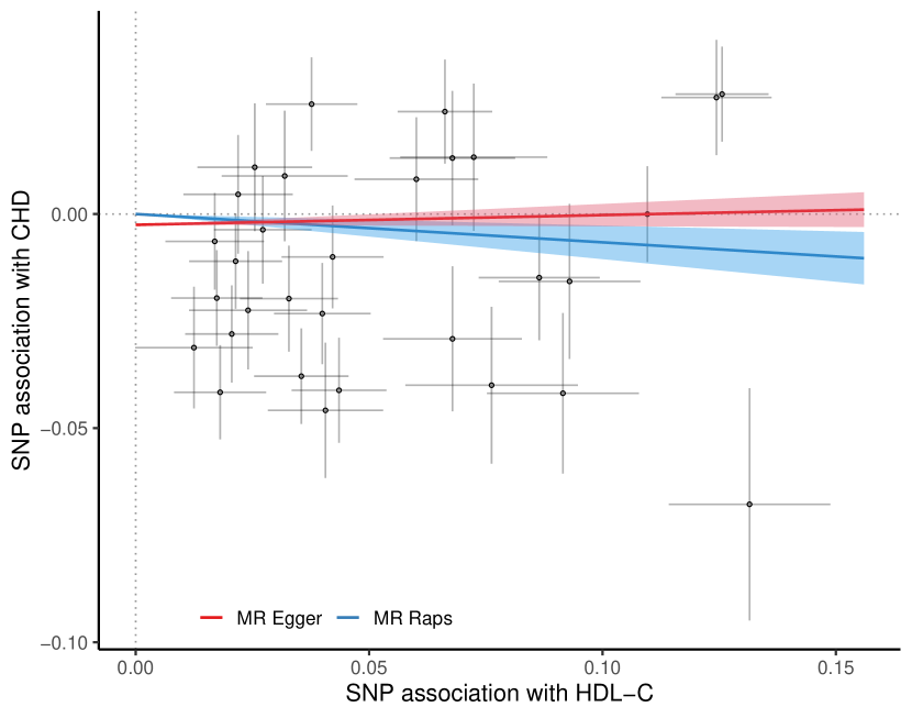
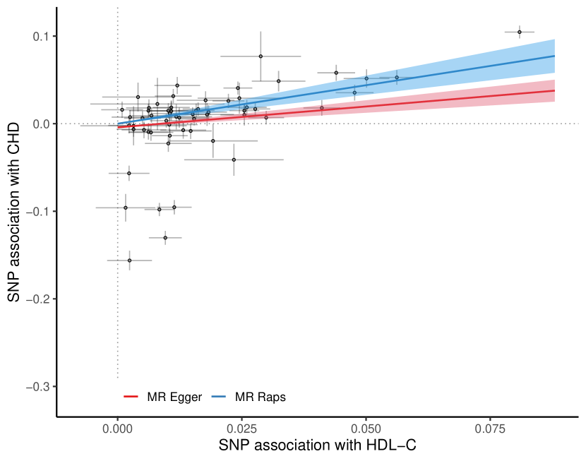
Using some of the latest large-scale GWAS datasets for HDL-C and CHD, we created a dataset to visualize and analyze the heterogeneity among potential genetic instruments for HDL (Figure 1). Each point in this plot shows the reported associations of a SNP with HDL-C and CHD in the GWAS (with standard error bars). Figure 1(a) shows straight lines across the origin whose slopes are obtained using MR-RAPS (Zhao et al., 2020) and MR-Egger (Bowden, Davey Smith and Burgess, 2015) which both assume a homogeneous effect of HDL-C on CHD.

If this assumption holds, the slopes in Figure 1(a) can be interpreted as the causal effects of HDL-C on CHD. However, it is clear from Figure 1(a) that the slopes estimated by both MR-RAPS and MR-Egger provide a poor fit to the scatterplot.

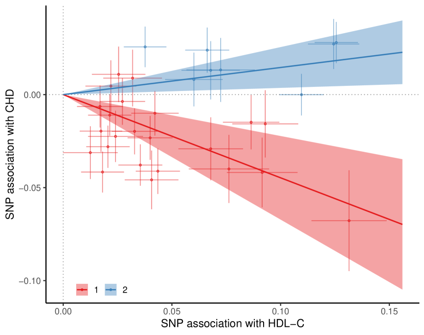
In this paper, we propose to fit this dataset using an alternative model where the SNPs have individual slopes that are drawn from a mixture distribution. This would be the case if there are several biological mechanisms involved in regulating HDL-C; see Section 3. In this example, MR-Path selects two clusters (shown in Figure 1(b)) which provides a much better fit to the data. See Section 7 for more detail about the data collection for this example and the results of our model.

(a) MR-RAPS & MR-Egger

(b) Proposed mixture model.

Figure 1: Scatterplot of HDL-CAD data and effect estimates. Left: Line/shaded region represents the causal effect estimate $\pm$ one standard error from MR-RAPS. Right: Lines/shaded regions represent heterogeneous causal effect estimates $\pm$ one standard deviation from our proposed mixture model.

1.2 Related work and our contributions

There have been several attempts to develop MR methods that allow for heterogeneous causal effects. We are also not the first to use mixture models for MR. The contamination mixture method proposed by Burgess et al. (2020) uses a two-component mixture model to distinguish between valid and invalid instruments. Similarly, the MR-Mix method (Qi and Chatterjee, 2019) uses a four-component mixture model to identify one group of valid instruments and three groups of invalid instruments which have either direct effects on both the exposure and outcome, direct effects on the outcome but no effect on the exposure, or no effect on both the exposure and outcome. However, the purpose of using mixture models in these approaches is not to identify different mechanisms but rather to provide a realistic model for the invalid instruments. In particular, they assume that a plurality of the instruments are valid and indicate an identical causal effect.

The only methods we are aware of that do not assume effect homogeneity and attempt to distinguish causal mechanisms are GRAPPLE (Wang et al., 2020), MR-Clust (Foley, Kirk and Burgess, 2019) and BESIDE-MR (Shapland, Zhao and Bowden, 2020). GRAPPLE proposes to use the local maximums of a robustified profile likelihood function (Zhao et al., 2020) to discover multiple mechanisms. However, GRAPPLE is only a visualization tool and does not attempt to explicitly model the different mechanisms. MR-Clust works by constructing a mixture model based on SNP-specific Wald estimators. Similar to our proposed method, MR-Clust does not make further assumptions about the number of clusters and the structure of each cluster. However, a major limitation of MR-Clust is its assumption that the SNP-specific Wald estimates are normally distributed, which is a poor approximation for weak instruments. A comparison between our proposed method and MR-Clust is provided in appendix D . BESIDE-MR is another related method that uses Bayesian model averaging. Although BESIDE-MR is initially motivated by averaging over the uncertainty in selecting the valid instruments, it can also be extended to allow for multiple clusters of instruments indicating different causal effects. However, BESIDE-MR is not a full likelihood approach because it uses the profile likelihood derived in Zhao et al. (2020) to eliminate the nuisance parameters related to the SNP-exposure effects.

Our paper makes two main contributions to this fast growing literature. First, there is a general lack of awareness that MR can be used to discover multiple biological mechanisms, partly due to the wide usage of the broad terminology “effect heterogeneity” to refer to several different phenomena—invalid instrument due to pleiotropy, effect modification/moderation by a covariate, and effect heterogeneity due to different causal mechanisms. In this article we introduce the concept of mechanistic heterogeneity for the last phenomenon and show that it can occur even if all the instruments are valid.

Our second contribution is a transparent mixture model, which we call MR-Path, to capture the mechanistic heterogeneity. Because our model is based on the SNP-exposure and SNP-outcome associations, it does not require the individual instruments to be strong. We develop a Monte-Carlo EM algorithm to fit this model. Since our Monte Carlo EM algorithm maximizes the full likelihood function for the latent mixture model, it has all the benefits of likelihood-based inference.

The rest of the paper is organized as follows. In section 2, we give a brief review of the standard assumptions in MR. In section 3, we introduce the concept of mechanistic heterogeneity. In section 4 we propose to model it with MR-Path. In section 5, we describe an Monte Carlo EM algorithm to fit MR-Path and discuss the relevant statistical inference and model selection procedures. We then study the performance of our Monte Carlo EM algorithm with two simulation studies in section 6 and apply it to two real data datasets (including the HDL-CHD example above) in section 7. We conclude the paper with some ending remarks in section 8.

2 MR as an instrumental variables method

The goal of MR is to estimate the causal effect of a risk exposure variable (X) on a disease outcome variable (Y). In particular, we may be interested in the causal effect of HDL cholesterol (X) on the risk of coronary heart disease (Y). Regression analyses between X and Y are typically biased by unobserved confounding variables $U$. MR uses $p$ genetic variants $Z_{1},\dots,Z_{p}$ as instrumental variables to obtain an unbiased causal effect estimate of X on Y. A genetic variant $Z$ is said to be a valid instrument for estimating the causal effect of $X$ on $Y$ if it satisfies the following assumptions:

Assumption 2.1 (Relevance).

It is associated with the risk exposure, i.e. $\text{Corr}(Z,X)\neq 0$.

Assumption 2.2 (Independence).

It must be independent of any unmeasured confounders that are associated with both the exposure and outcome, i.e. $Z\ \rotatebox[origin={c}]{90.0}{$\models$}\ U$.

Assumption 2.3 (Exclusion restriction).

It affects the outcome only through the risk exposure, i.e. $Z\ \rotatebox[origin={c}]{90.0}{$\models$}\ Y\ |\ X$.

Figure 2: A directed acyclic graph (DAG) illustrating the core assumptions for a valid instrument.

Figure 2 provides a graphical representation of these assumptions. The independence assumption is usually guaranteed by Mendel’s law of random assortment of genes. The relevance assumption is justified if genetic variants are chosen to be genome-wide significant. Among the three assumptions, the exclusion restriction (ER) assumption is the most problematic due to pleiotropy. Assessment of the IV assumptions and sensitivity analysis in MR are discussed by Burgess et al. (2017). In the MR literature, it is common to assume the following linear structural equation model for the exposure and outcome variables (Bowden et al., 2017):

$$X =\sum_{i=1}^{p}\theta_{X_{i}}Z_{i}+\eta_{X}U+E_{X},$$ (1)

$$Y =\beta X+\sum_{i=1}^{p}\alpha_{i}Z_{i}+\eta_{Y}U+E_{Y},$$ (2)

where $\eta_{X}$ and $\eta_{Y}$ are confounding effects and $E_{X}$ and $E_{Y}$ are random noise terms acting on $X$ and $Y$ respectively. The causal effect between $X$ and $Y$ is given by the parameter $\beta$. The true marginal association between $X$ and $Z_{i}$ is given by $\theta_{X_{i}}$. The direct effect of $Z_{i}$ on $Y$ is given by $\alpha_{i}$. Assumption 2.1 implies $\theta_{X_{i}}\neq 0$ and assumption 2.2 implies $Z_{1},\dots,Z_{p}\ \rotatebox[origin={c}]{90.0}{$\models$}\ U,E_{X},E_{Y}$. Under this model, the exclusion restriction assumption is violated if $\alpha_{i}\neq 0$. In particular, this can occur if $Z_{i}$ affects $Y$ through a mechanism unrelated to $X$ (see fig. 3(a) for illustration). Plugging eq. 1 into eq. 2, we obtain

$$Y=\sum_{i=1}^{p}\Big{(}\beta\theta_{X_{i}}+\alpha_{i}\Big{)}Z_{i}+(\eta_{X}+\eta_{Y})U+(E_{X}+E_{Y})=\sum_{i=1}^{p}\theta_{Y_{i}}Z_{i}+E_{Y}^{\prime},$$ (3)

where $\theta_{Y_{i}}=\beta\theta_{X_{i}}+\alpha_{i}$ gives the true marginal association between $Y$ and $Z_{i}$ and $E_{Y}^{\prime}$ is a random noise term that is independent of $Z_{i}$. In summary-data MR, we usually observe the estimated SNP-exposure effect $\hat{\theta}_{X_{i}}$, with standard error $\sigma_{X_{i}}$, and the estimated SNP-outcome effect $\hat{\theta}_{Y_{i}}$, with standard error $\sigma_{Y_{i}}$, for SNP $i=1,\dots,p$. These estimated effects are typically computed from two different samples using linear or logistic regression. If we assume the genetic variants $Z_{1},\dots,Z_{p}$ satisfy the exclusion restriction assumption, in other words $\alpha_{1}=\dots=\alpha_{p}=0$, then the causal effect parameter $\beta$ can be estimated consistently with the inverse-variance-weighted estimator Burgess, Butterworth and Thompson (2013). A more robust approach is to perform error-in-variables regression of $\hat{\theta}_{Y_{i}}$ on $\hat{\theta}_{X_{i}}$ (Zhao et al., 2020). We adopt this approach in MR-Path. If the exclusion restriction assumption is violated for some SNPs, then the causal effect parameter $\beta$ cannot be identified without further assumptions on $\alpha_{i}$. For example, Zhao et al. (2020) assumes that $\alpha_{i}\sim N(0,\tau^{2})$ for most genetic variants so that the direct effects are balanced out.

3 Mechanistic heterogeneity in MR

(a) Scenario 1: Multiple pathways of horizontal pleiotropy.

(b) Scenario 2: Multiple mechanisms for the exposure $X$.

Figure 3: Two scenarios of mechanistic heterogeneity

Table 1: Ratio estimands using different instruments in the two scenarios in Figure 3. Directed acyclic graphs in Figure 3 are interpreted as linear structural equation models.

Instruments $Z$	Pathway $M$	Effect of $M$ on $X$	Effect of $M$ on $Y$	Wald estimand
Scenario 1
$Z_{1,1},\dotsc,Z_{1,p_{1}}$	$M_{1}$	$\theta_{1}$	$\theta_{1}\beta$	$\beta$
$Z_{2,1},\dotsc,Z_{2,p_{2}}$	$M_{2}$	$\theta_{2}$	$\theta_{2}\beta+\alpha_{2}$	$\beta+\alpha_{2}/\theta_{2}$
$Z_{3,1},\dotsc,Z_{3,p_{3}}$	$M_{3}$	$\theta_{3}$	$\theta_{3}\beta+\alpha_{3}$	$\beta+\alpha_{3}/\theta_{3}$
Scenario 2
$Z_{1,1},\dotsc,Z_{1,p_{1}}$	$M_{1}$	$\theta_{1}$	$\theta_{1}\beta_{1}$	$\beta_{1}$
$Z_{2,1},\dotsc,Z_{2,p_{2}}$	$M_{2}$	$\theta_{2}$	$\theta_{2}\beta_{2}$	$\beta_{2}$
$Z_{3,1},\dotsc,Z_{3,p_{3}}$	$M_{3}$	$\theta_{3}$	$\theta_{3}\beta_{3}$	$\beta_{3}$

The assumption that the direct effect $\alpha_{i}$ is iid normally distributed does not take into account the possibility that genetic variation often affects phenotypic traits through separate biological pathways. In this section we show that such behaviour may lead to a clustering phenomenon where SNPs belonging to the same pathway would indicate similar causal effects in an MR analysis. This is what we call “mechanistic heterogeneity” in MR.

3.1 Two origins of mechanistic heterogeneity

Consider Figure 3 which contains two scenarios of mechanistic heterogeneity that motivate the latent mixture model. In both scenarios, genetic variants are grouped into three biological pathways, $M_{1}$, $M_{2}$, and $M_{3}$, that affect the exposure $X$ and outcome $Y$ differently. In the first scenario (Figure 3(a)), all three pathways affect $X$ in the same way but have different direct effects on $Y$. In particular, the first pathway $M_{1}$ does not have any direct effect on $Y$ not mediated by $X$, so the instruments $Z_{1,1},\dotsc,Z_{1,p_{1}}$ associated with it are all valid IVs. In the second scenario in Figure 3(b), the three pathways affect different components of the exposure $X$ which also have different causal effects on the outcome $Y$. If we interpret the diagrams in Figure 3 as linear structural equations (like Figure 2 for (1) and (2)), we can derive the so-called Wald estimand (ratio of $\theta_{Y}$ and $\theta_{X}$) for each instrument (Table 1). In both scenarios in Figure 3, genetic instruments on the same pathway have the same Wald estimand $\theta_{Y}/\theta_{X}$, while instruments across different pathways generally have different estimands.

Therefore, we may reach completely different conclusions when using instruments on different pathways in the MR analysis. In reality, mechanistic heterogeneity can be more complicated than the basic scenarios in Figure 3. For example, another pathway can affect some components of $X$ and also have direct effect on $Y$. We study the robustness of our proposed method when horizontal pleiotropy and multiple mechanisms are simultaneously present in appendix E. It is also worthwhile to point out that mechanistic heterogeneity can arise even when all the IVs are perfectly valid; an example is Scenario 2 in Figure 3.

3.2 Relationship to local average treatment effect

The above introduction of mechanistic heterogeneity is entirely based on linear structural equation models. Next we show that the same clustering phenomenon can also happen when there is nonlinearity. Consider the causal diagram in Figure 3(a) without the $M_{2}\to Y$ and $M_{3}\to Y$ edges, so all the instruments $Z_{1,1},\dotsc,Z_{3,p_{3}}$ are valid (satisfy Assumptions 2.1, 2.2 and 2.3). Suppose the variables satisfy the nonparametric structural equation model (NPSEM) with independent errors (Pearl, 2009) according to Figure 3(a), so the counterfactuals of $M_{k},k=1,2,3$, $X$, and $Y$ can be defined using the NPSEM. For example, we use $Y(X=1)$ to denote the counterfactual outcome under the intervention $X=1$. To simplify our illustration below, we assume $Z_{1,1},\dotsc,Z_{3,p_{3}}$, $M_{1},M_{2},M_{3}$, and $X$ are all binary variables.

It is well known that if the instrument $Z_{k,j}$ is valid and the counterfactuals of the exposure $X$ satisfy the monotonicity assumption $X(Z_{k,j}=1)\geq X(Z_{k,j}=0)$, the Wald estimand for instrument $Z_{k,j}$ is equal to the so-called local average treatment effect, $\mathbb{E}[Y(X=1)-Y(X=0)\mid X(Z_{k,j}=1)>X(Z_{k,j}=0)]$ (Angrist, Imbens and Rubin, 1996). Notice that this interpretation of the IV analysis does not require linearity of the structural equation model. Suppose we further assume the effect of $Z$ on $M$ is monotone, $M_{k}(Z_{k,j}=1)\geq M_{k}(Z_{k,j}=0),$ and the effect of $M$ on $X$ is monotone, $X(M_{k}=1)\geq X(M_{k}=0)$. Using the properties of counterfactuals and the fact in Figure 3(a) that $Z_{k,j}$ affects $X$ entirely through $M_{k}$, we get

$$X(Z_{k,j}=z)=X(Z_{k,j}=z,M_{k}=M_{k}(Z_{k,j}=z))=X(M_{k}=M_{k}(Z_{k,j}=z)).$$

Thus, using the assumption that $X$ and $M_{k}$ are binary,

$$\begin{split}&\mathbb{E}\big{[}Y(X=1)-Y(X=0)\mid X(Z_{k,j}=1)>X(Z_{k,j}=0)\big{]}\\ =&\mathbb{E}\big{[}Y(X=1)-Y(X=0)\mid X\big{(}M_{k}=M_{k}(Z_{k,j}=1)\big{)}>X\big{(}M_{k}=M_{k}(Z_{k,j}=0)\big{)}\big{]}\\ =&\mathbb{E}\big{[}Y(X=1)-Y(X=0)\mid X(M_{k}=1)>X(M_{k}=0),M_{k}(Z_{k,j}=1)>M_{k}(Z_{k,j}=0)\big{]}\\ =&\mathbb{E}\big{[}Y(X=1)-Y(X=0)\mid X(M_{k}=1)>X(M_{k}=0)\big{]}.\end{split}$$ (4)

The last equality above uses

$$\{M_{k}(Z_{k,j}=0),M_{k}(Z_{k,j}=1)\}\,\rotatebox[origin={c}]{90.0}{$\models$}\,\{X(M_{k}=0),X(M_{k}=1),Y(X=0),Y(X=1)\}.$$

This counterfactual independence follows from expressing the counterfactuals using the NPSEM and the assumption that the different structural equations have independent errors.

The significance of (4) is that, if the counterfactuals of $M$ and $X$ satisfy the monotonicity assumption, the local average treatment effect corresponding to $Z_{k,j}$ only depends on the mechanism index $k$. This shows that the clustering of the Wald esimand in Section 3.1 not only occurs in linear structural equation models but also in certain nonlinear models. These examples demonstrate the importance of identifying mechanistic heterogeneity to correctly interpret MR studies.

4 MR-Path: A latent mixture model for mechanistic heterogeneity

Motivated by the observations in the previous section, we propose a latent mixture model to discover mechanistic heterogeneity using summary GWAS data. In essence, this model assumes that each genetic variant has a specific causal effect and the genetic variants on the same biological pathway have similar variant-specific causal effects and form clusters. The mean of each cluster corresponds to the Wald estimand of that pathway (last column in table 1). These assumptions, along with standard assumptions for summary-data MR literature, are introduced below. A graphical model formulation of MR-Path is shown in fig. 4.

Assumption 4.1 (Error-in-variables regression).

The observed instrument-exposure and instrument-outcome associations are distributed as

$$\begin{pmatrix}\hat{\theta}_{X_{i}}\\ \hat{\theta}_{Y_{i}}\end{pmatrix}\overset{\text{indep.}}{\sim}N\Big{(}\begin{pmatrix}\theta_{X_{i}}\\ \beta_{i}\theta_{X_{i}}\end{pmatrix},\begin{pmatrix}\sigma_{X_{i}}^{2}&0\\ 0&\sigma_{Y_{i}}^{2}\end{pmatrix}\Big{)},\quad i=1,\dots,p,$$ (5)

where $\sigma_{X_{i}}$, $\sigma_{Y_{i}}$ are (fixed) measurement errors.

In this assumption, the variant-specific causal effects are given by $\beta_{i}$. The normality assumption is justified because $\hat{\theta}_{X_{i}}$ and $\hat{\theta}_{Y_{i}}$ are typically linear (or logistic) regression coefficients which are computed in GWAS with a large sample size. Independence between $\hat{\theta}_{X_{i}}$ and $\hat{\theta}_{Y_{i}}$ for each SNP is justified if they are from GWAS conducted with non-overlapping samples. Independence of the estimated effects across different SNPs is a reasonable assumption if we select SNPs that are uncorrelated by using linkage disequilibrium clumping. Although independence between SNPs does not imply the estimated effects are uncorrelated, the correlation between the estimated effects are typically negligible (Zhao et al., 2020).

Assumption 4.2 (Mixture model for mechanistic heterogeneity).

$$\xi_{i} \sim\text{Categorical }(\pi_{1},\dots,\pi_{K}),$$ (6)

$$\beta_{i}|\xi_{i}=k \sim N(\mu_{k},\sigma_{k}^{2}),\quad k=1,\ldots,K.$$ (7)

We assume a Gaussian mixture model for the variant-specific (latent) causal effects $\beta_{i}$ to probabilistically cluster genetic variants with similar causal effects. An indicator variable for cluster membership of SNP $i$ is given by $\xi_{i}$. We can compute the posterior distribution of $\xi_{i}$ and $\beta_{i}$ to summarize our knowledge of these variant-specific latent variables based on data (see section 5.4). The $K$ clusters represent different causal mechanisms where the cluster means $\mu_{k}$, for $k=1,\dots,K$, identify the average causal effects for each mechanism. The cluster proportions $\pi_{k}$ give us the proportion of genetic variants associated with each mechanism. The cluster variances $\sigma_{k}^{2}$ quantify uncertainty within each mechanism. Therefore, the parameters of interest in MR-Path are given by $\varphi=\{\pi_{k},\mu_{k},\sigma_{k}^{2}:k=1,\dots,K\}$. Note that eq. 7 assumes the Wald estimand corresponding to each genetic instrument $\beta_{i}$ is allowed to fluctuate around the cluster means $\mu_{k}$’s. The cluster variance $\sigma_{k}^{2}$ thus captures the within-cluster heterogeneity due to unaccounted direct effects of the instruments on the outcome. This is similar to making the InSIDE (INstrument Strength Independent of Direct Effect) assumption (Bowden, Davey Smith and Burgess, 2015) within each mixture component. The number of clusters $K$ is unknown but can be chosen based on heuristics and domain knowledge or estimated from data—see section 5.5 for a model selection criterion for choosing $K$. Note that assumption 4.1 implies $\beta_{i}$ and $\theta_{X_{i}}$ are marginally independent but conditionally dependent given the observed data. This can be deduced from the graphical model in fig. 4 (chapter 8 in Bishop (2006)).

Figure 4: Graphical model formulation of MR-Path. Observed data is represented by gray circles; latent variables are represented by white circles; and model parameters are represented by diamonds.

5 Statistical inference for MR-Path

In order to fit MR-Path to gain insight into mechanistic heterogeneity, we proceed by discussing three inference procedures. First, we describe our implementation of the EM algorithm for obtaining a maximum likelihood estimate of $\varphi$ and point out the challenges and our solutions for the expectation step. Second, we discuss approximate confidence intervals for $\varphi$ obtained by computing and inverting the observed information matrix. Lastly, we go into how $K$ can be selected from data using a modified Bayesian Information criterion (BIC). Let $\mathbf{D}=\{(\hat{\theta}_{X_{i}},\sigma_{X_{i}},\hat{\theta}_{Y_{i}},\sigma_{Y_{i}}):i=1,\dots,p\}$ denote the observed data and let $\mathbf{\Theta}=\{(\theta_{X_{i}},\beta_{i},\xi_{i}):i=1,\dots,p\}$ denote the set of latent variables.

5.1 Overview of the EM Algorithm

The Expectation-Maximization (EM) algorithm is an iterative procedure commonly used to perform maximum likelihood estimation in latent variable models. To define the EM algorithm for MR-Path, we derive two important model quantities: the complete-data log likelihood and the conditional posterior of the latent variables $\mathbf{\Theta}$, given parameters $\varphi$. The latter is used to compute the Q-function in the expectation step. Let $\phi(\cdot;\mu,\sigma^{2})$ denote the density of $N(\mu,\sigma^{2})$. We make the additional model assumption that $\theta_{X_{i}}\sim N(\nu_{x},\lambda_{x}^{2})$. It follows that the complete-data log likelihood for MR-Path is given by

$$l(\varphi;\mathbf{\Theta}):=\sum_{i=1}^{p}l_{i}(\varphi;\theta_{X_{i}},\beta_{i},\xi_{i}),$$ (8)

where

$$l_{i}(\varphi;\theta_{X_{i}},\beta_{i},\xi_{i})\propto\log\phi(\theta_{X_{i}};\nu_{x},\lambda_{x}^{2})+\sum_{k=1}^{K}Z_{ik}\big{[}\log\pi_{k}+\log\phi(\beta_{i};\mu_{k},\sigma_{k}^{2})\big{]}$$ (9)

and $Z_{ik}=1$, if $\xi_{i}=k$, and $0$ otherwise. The conditional posterior of the latent variables given $\varphi$ can be decomposed as

$$P(\mathbf{\Theta}|\mathbf{D},\varphi):= \prod_{i=1}^{p}P(\beta_{i},\xi_{i},\theta_{X_{i}}|\hat{\theta}_{X_{i}},\hat{\theta}_{Y_{i}},\varphi)$$

$$= \prod_{i=1}^{p}\prod_{k=1}^{K}\big{[}P(\xi_{i}=k|\beta_{i},\varphi)\big{]}^{Z_{ik}}P(\beta_{i}|\theta_{X_{i}},\hat{\theta}_{Y_{i}},\varphi)P(\theta_{X_{i}}|\hat{\theta}_{X_{i}},\hat{\theta}_{Y_{i}},\varphi),$$ (10)

where $P(\xi_{i}=k|\beta_{i},\varphi)$ and $P(\beta_{i}|\theta_{X_{i}},\hat{\theta}_{Y_{i}},\varphi)$ are available in closed-form and are given by

$$P(\xi_{i}=k|\beta_{i},\varphi) =\frac{\pi_{k}\phi(\beta_{i};\mu_{k},\sigma_{k}^{2})}{\sum_{j=1}^{K}\pi_{j}\phi(\beta_{i};\mu_{j},\sigma_{j}^{2})},$$ (11)

$$P(\beta_{i}|\theta_{X_{i}},\hat{\theta}_{Y_{i}},\varphi) =\sum_{k=1}^{K}\tilde{\pi}_{ik}\phi(\beta_{i};\tilde{\mu}_{ik},\tilde{\sigma}_{ik}^{2});$$ (12)

where

$$\tilde{\pi}_{ik}=\pi_{k}\Big{[}2\pi\Big{(}\frac{\theta_{X_{i}}^{2}}{\sigma_{Y_{i}}^{2}}+\frac{1}{\sigma_{k}^{2}}\Big{)}^{-1}\Big{]}^{1/2},\quad\tilde{\sigma}_{ik}^{2}=\Big{(}\frac{1}{\sigma_{k}^{2}}+\frac{\theta_{X_{i}}^{2}}{\sigma_{Y_{i}}^{2}}\Big{)}^{-1},\quad\tilde{\mu}_{ik}=\tilde{\sigma}_{ik}^{2}\Big{(}\frac{\hat{\theta}_{Y_{i}}\theta_{X_{i}}}{\sigma_{Y_{i}}^{2}}+\frac{\mu_{k}}{\sigma_{k}^{2}}\Big{)}.$$ (13)

Details for the derivation of $P(\beta_{i}|\theta_{X_{i}},\hat{\theta}_{Y_{i}},\varphi)$ are given in appendix A. Unfortunately, instead of having an analytical solution, the probability density $P(\theta_{X_{i}}|\hat{\theta}_{X_{i}},\hat{\theta}_{Y_{i}},\varphi)$ is known only up to a multiplicative constant given by

$$P(\theta_{X_{i}}|\hat{\theta}_{X_{i}},\hat{\theta}_{Y_{i}},\varphi) \propto P(\theta_{X_{i}}|\hat{\theta}_{X_{i}},\varphi)P(\hat{\theta}_{Y_{i}}|\theta_{X_{i}},\varphi)$$

$$=\phi(\theta_{X_{i}};m_{X_{i}},\lambda_{X_{i}}^{2})\sum_{k=1}^{K}\pi_{k}\phi(\hat{\theta}_{Y_{i}};\theta_{X_{i}}\mu_{k},\theta_{X_{i}}^{2}\sigma_{k}^{2}+\sigma_{Y_{i}}^{2}),$$ (14)

where

$$\lambda_{X_{i}}^{2} =\Big{(}\frac{1}{\sigma_{X_{i}}^{2}}+\frac{1}{\lambda_{x}^{2}}\Big{)}^{-1},\quad m_{X_{i}}=\lambda_{X_{i}}^{2}\Big{(}\frac{\hat{\theta}_{X_{i}}}{\sigma_{X_{i}}^{2}}+\frac{\nu_{x}}{\lambda_{x}^{2}}\Big{)}.$$

The EM algorithm starts with initial values for the parameter estimates $\varphi^{(0)}$. Each iteration $t=1,2,\dots$ of the EM algorithm consists of an expectation step (E-step) and a maximization (M-step). The E-step involves computing the Q-function, defined as the expectation of the complete-data log likelihood with respect to the conditional posterior of the latent variables given the previous iterations parameter estimates. Specifically, the E-step can be represented by

$$Q(\varphi,\varphi^{(t-1)})=E\big{[}l(\varphi;\mathbf{\Theta})|\mathbf{D},\varphi^{(t-1)}\big{]},$$ (15)

where the expectation is taken with respect to $P(\mathbf{\Theta}|\mathbf{D},\varphi)$. The M-step consists of computing an update of the parameter estimates for the current iteration as the value that maximizes the Q-function. In other words, the M-step involves

$$\varphi^{(t)}=\underset{\varphi}{\text{arg max }}Q(\varphi,\varphi^{(t-1)}).$$ (16)

The EM algorithm guarantees the likelihood is non-decreasing across iterations—ascent property—and is theoretically guaranteed, under mild regularity conditions, to converge to a local optimum (Wu, 1983). In practice, a commonly used heuristic for determining whether the EM algorithm has converged is when the increase in the Q-function from the previous iteration is less than a specified threshold. Unfortunately, since $P(\mathbf{\Theta}|\mathbf{D},\varphi)$ is only known up to a multiplicative constant, the Q-function for MR-Path cannot be computed analytically. In the next section, we discuss our implementation of a variant of the EM algorithm where the Q-function in the E-step is approximated using Monte-Carlo methods—the Monte-Carlo EM (MC-EM) algorithm.

5.2 Implementation of the Monte-Carlo EM Algorithm

The MC-EM algorithm allows us to perform maximum likelihood estimation in latent variable models where the Q-function cannot be computed analytically but can be approximated using Monte-Carlo methods. In section 5.2.1, we describe an importance sampling (IS) scheme for approximating the Q-function in MR-Path. The main drawback of the MC-EM algorithm is that Monte-Carlo error accrued from approximating the Q-function may cause the algorithm to not converge (Neath, 2013). More precise approximations of the Q-function are needed as the M-step updates approach a local optimum. Furthermore, the MC-EM algorithm does not satisfy the ascent property of the vanilla EM algorithm. A simple solution to these issues is to set the number of Monte-Carlo samples used to approximate the Q-function (MC sample size) to be very large or increase the MC sample size by a deterministic large amount at each iteration. However, this may not be computationally feasible, thus creating a trade-off between statistical consistency and computational efficiency. In section 5.2.2, we discuss an automated data-driven procedure introduced by Caffo, Jank and Jones (2005) that guarantees the ascent property is satisfied with high probability by assessing Monte-Carlo error at the end of each iteration and increasing the MC sample size accordingly. The runtimes for the proposed MC-EM algorithm applied to the two examples in section 7 are provided in appendix F.

5.2.1 Monte-Carlo E-step using Importance Sampling

The decomposition of $P(\mathbf{\Theta}|\mathbf{D},\varphi)$ in eq. 10 suggests that we can obtain importance samples from $P(\mathbf{\Theta}|\mathbf{D},\varphi)$ by first drawing samples of $\{\theta_{X_{i}}\}$ from an importance (proposal) distribution. Given importance samples of $\{\theta_{X_{i}}\}$, we can obtain importance samples of $\{\beta_{i}\}$ and $\{\xi_{i}\}$ by directly sampling from $\prod_{i=1}^{p}P(\beta_{i}|\theta_{X_{i}},\hat{\theta}_{X_{i}},\varphi)$ and $\prod_{i=1}^{p}P(\xi_{i}|\beta_{i},\varphi)$, which are available in closed form in eq. 11 and eq. 12. Then, we can estimate the Q-function with a sum of the complete-data log-likelihood evaluated at the samples weighted by the importance weights.

Choosing an importance distribution that yields an efficient sampling procedure is a non-trivial task that depends on the form of the target distribution (see Tokdar and Kass (2010) for a review). In our case, the target distribution is $\prod_{i=1}^{p}P(\theta_{X_{i}}|\hat{\theta}_{X_{i}},\hat{\theta}_{Y_{i}},\varphi)$ so a sensible choice for an importance (proposal) distribution would be $\prod_{i=1}^{p}P(\theta_{X_{i}}|\hat{\theta}_{X_{i}},\varphi)$, the posterior distribution of $\{\theta_{X_{i}}\}$ given only $\{\hat{\theta}_{X_{i}}\}$ instead of the full data $\{\hat{\theta}_{X_{i}},\hat{\theta}_{Y_{i}}\}$ which has a closed form given in eq. 14. This choice of importance distribution yields importance weights that are bounded and have a finite variance.

More precisely, let $m_{t}$ denote the number of desired importance samples at iteration $t$ and $\tilde{\varphi}^{(t-1)}$ denote the MC-EM update from iteration $t-1$. For each $i=1,\dots,p$ and $j=1,\dots,m_{t}$, suppose $\theta_{X_{i}}^{j}\sim P(\theta_{X_{i}}|\hat{\theta}_{X_{i}},\varphi^{(t-1)})$, $\beta_{i}^{j}\sim P(\beta_{i}|\theta_{X_{i}},\hat{\theta}_{Y_{i}},\varphi^{(t-1)})$, and $\xi_{i}^{j}\sim P(\xi_{i}|\beta_{i},\varphi^{(t-1)})$. From eq. 14, we have that the unnormalized importance weights are given by

$$w_{i}^{j}=P(\hat{\theta}_{Y_{i}}|\theta_{X_{i}}^{j},\tilde{\varphi}^{(t-1)})=\sum_{k=1}^{K}\tilde{\pi}_{k}^{(t-1)}\phi\Big{(}\hat{\theta}_{Y_{i}};\theta_{X_{i}}^{j}\tilde{\mu}_{k}^{(t-1)},(\theta_{X_{i}}^{j})^{2}\tilde{\sigma}_{k}^{2(t-1)}+\sigma_{Y_{i}}^{2}\Big{)}$$ (17)

for $j=1,\dots,M$. It can be shown that $0\leq w_{i}^{j}\leq\big{(}2\pi\sigma_{Y_{i}}^{2}\big{)}^{-1/2}$ (proof is provided in appendix B). Let $\bar{w}_{i}^{j}=w_{i}^{j}/\sum_{j=1}^{m_{t}}w_{i}^{j}$ be the normalized importance weights. The IS estimate of the Q-function at iteration $t$ is given by

$$\tilde{Q}(\varphi,\tilde{\varphi}^{(t-1)};m_{t})=\sum_{i=1}^{p}\sum_{j=1}^{m_{t}}\bar{w}_{i}^{j}l_{i}^{j}(\varphi),$$ (18)

where

$$l_{i}^{j}(\varphi)=l_{i}(\varphi;\theta_{X_{i}}^{j},\beta_{i}^{j},\xi_{i}^{j}),$$

and $l_{i}$ is defined in eq. 9. Consequently, the MC-EM update of the model parameters at iteration $t$ approximated with Monte-Carlo sample size $m_{t}$ is given by

$$\tilde{\varphi}^{(t,m_{t})}=\underset{\varphi}{\text{arg max }}\tilde{Q}(\varphi,\tilde{\varphi}^{(t-1)};m_{t}).$$

5.2.2 Ascent-Based Monte-Carlo EM

At the end of each MC-EM iteration, the ascent-based MC-EM algorithm (Caffo, Jank and Jones, 2005) performs a hypothesis test to determine whether the Q-function has increased from the previous iteration. If there is not sufficient evidence that suggests the Q-function has increased, we reject the current iteration’s M-step and repeat the iteration with a larger MC sample size. In this section, we will describe this procedure concretely for our inference problem.

Define the change in the Q function at iteration $t$ of MC-EM as

$$\Delta Q(\tilde{\varphi}^{(t,m_{t})},\tilde{\varphi}^{(t-1)}):=Q(\tilde{\varphi}^{(t,m_{t})},\tilde{\varphi}^{(t-1)})-Q(\tilde{\varphi}^{(t-1)},\tilde{\varphi}^{(t-1)}).$$ (19)

After obtaining $\tilde{\varphi}^{(t,m_{t})}$ in the M-step, we are interested in performing the following hypothesis test at a specified significance level $\alpha$:

$$H_{0}:\Delta Q(\tilde{\varphi}^{(t,m_{t})},\tilde{\varphi}^{(t-1)})=0,$$ (20)

$$H_{A}:\Delta Q(\tilde{\varphi}^{(t,m_{t})},\tilde{\varphi}^{(t-1)})>0.$$

If we reject $H_{0}$, then we accept $\tilde{\varphi}^{(t,m_{t})}$ and move on to the next iteration. If we fail to reject $H_{0}$, then we reject $\tilde{\varphi}^{(t,m_{t})}$ and repeat the current iteration with a larger Monte-Carlo sample size. The change in the Q function in eq. 19 can be approximated using

$$\Delta\tilde{Q}(\tilde{\varphi}^{(t,m_{t})},\tilde{\varphi}^{(t-1)})\approx\sum_{i=1}^{p}\sum_{j=1}^{m_{t}}w_{i}^{j}\Lambda_{ij}^{(t)}$$ (21)

where

$$\Lambda_{ij}^{(t)}=l_{i}^{j}(\tilde{\varphi}^{(t,m_{t})})-l_{i}^{j}(\tilde{\varphi}^{(t-1)}).$$ (22)

It was shown in Caffo, Jank and Jones (2005) that under $H_{0}$,

$$\sqrt{m_{t}}\Delta\tilde{Q}(\tilde{\varphi}^{(t,m_{t})},\tilde{\varphi}^{(t-1)})\overset{d}{\rightarrow}N(0,\eta^{2})$$ (23)

as $m_{t}\rightarrow\infty$, where $\sigma^{2}$ depends on the sampling procedure used. We can obtain an estimate of $\eta^{2}$, $\hat{\eta}^{2}$, by computing the variance of the importance sampling estimate in eq. 21 (details provided in appendix C). Therefore, we can reject $H_{0}$ with approximate significance level $\alpha$ if

$$\Delta\tilde{Q}(\tilde{\varphi}^{(t,m_{t})},\tilde{\varphi}^{(t-1)})-z_{\alpha}\frac{\hat{\eta}}{m_{t}}>0$$

where $z_{\alpha}$ is the $(1-\alpha)^{\text{th}}$ quantile of the standard normal distribution. If we fail to reject $H_{0}$, we repeat iteration $t$ with a larger $m_{t}$ until we are able to reject $H_{0}$. Similarly, a convenient stopping criterion is obtained by testing

$$H_{A}:\Delta Q(\tilde{\varphi}^{(t,m_{t})},\tilde{\varphi}^{(t-1)})<\epsilon$$

at a specified significance level $\gamma$ and threshold $\epsilon$. We can reject $H_{0}$ with approximate significance level $\gamma$ and determine MC-EM has converged if

$$\Delta\tilde{Q}(\tilde{\varphi}^{(t,m_{t})},\tilde{\varphi}^{(t-1)})+z_{\gamma}\frac{\hat{\eta}}{m_{t}}<\epsilon.$$

5.3 Approximate Confidence Intervals

To quantify uncertainty of the parameter estimates obtained using the MC-EM algorithm, we adapt the method in (Louis, 1982) for computing the observed information matrix in the EM framework. Standard errors, and therefore approximate confidence intervals, can then be obtained by inverting the observed information matrix. By a result presented in (Louis, 1982), the observed information matrix at a point $\varphi^{*}$ can be computed by

$$I(\varphi^{*})=\Big{\{}E\Big{[}-\frac{\partial^{2}l(\varphi)}{\partial\varphi\partial\varphi^{T}}\Big{|}\mathbf{D},\varphi^{*}\Big{]} -E\Big{[}\Big{(}\frac{\partial l(\varphi)}{\partial\varphi}\frac{\partial l(\varphi)}{\partial\varphi^{T}}\Big{)}\Big{|}\mathbf{D},\varphi^{*}\Big{]}$$

$$+E\Big{[}\frac{\partial l(\varphi)}{\partial\varphi}\Big{|}\mathbf{D},\varphi^{*}\Big{]}E\Big{[}\frac{\partial l(\varphi)}{\partial\varphi^{T}}\Big{|}\mathbf{D},\varphi^{*}\Big{]}\Big{\}}\Big{|}_{\varphi=\varphi^{*}}$$ (24)

where the dependence of $\mathbf{D}$, $\mathbf{\Theta}$ in the log-likelihood has been suppressed for notational convenience. Let $\hat{\varphi}$ denote the final MC-EM parameter estimate and suppose $\{\theta_{X_{i}}^{j}$, $\beta_{i}^{j}$, $\xi_{i}^{j}:j=1,\dots,M\}$ are now importance samples from $P(\theta_{X_{i}},\beta_{i},\xi_{i}|\mathbf{D},\hat{\varphi})$ with (normalized) weights $\{w_{i}^{j}\}$. The first and third expectations in eq. 24 can be approximated by

$$E\Big{[}-\frac{\partial^{2}l(\varphi)}{\partial\varphi\partial\varphi^{T}}\Big{|}\mathbf{D},\varphi\Big{]} \approx\sum_{i=1}^{p}\sum_{j=1}^{M}w_{i}^{j}\frac{\partial^{2}l_{i}^{j}(\varphi)}{\partial\varphi\partial\varphi^{T}},$$

$$\text{and}\quad E\Big{[}\frac{\partial l(\varphi)}{\partial\varphi}\Big{|}\mathbf{D},\varphi\Big{]} \approx\sum_{i=1}^{p}\sum_{j=1}^{M}w_{i}^{j}\frac{\partial l_{i}^{j}(\varphi)}{\partial\varphi}.$$

The second expectation in eq. 24 can be approximated by

$$E\Big{[}\Big{(}\frac{\partial l(\varphi)}{\partial\varphi}\frac{\partial l(\varphi)}{\partial\varphi^{T}}\Big{)}\Big{|}\mathbf{D},\varphi^{*}\Big{]} =\sum_{i=1}^{p}E\Big{[}\Big{(}\frac{\partial}{\partial\varphi}l_{i}(\varphi)\Big{)}\Big{(}\frac{\partial}{\partial\varphi}l_{i}(\varphi)\Big{)}^{T}\Big{]}+2\sum_{i<n}E\Big{[}\frac{\partial}{\partial\varphi}l_{i}(\varphi)\Big{]}E\Big{[}\frac{\partial}{\partial\varphi}l_{n}(\varphi)\Big{]}^{T}$$

$$\approx\sum_{i=1}^{p}\sum_{j=1}^{M}w_{i}^{j}\frac{\partial l_{i}^{j}(\varphi)}{\partial\varphi}\frac{\partial l_{i}^{j}(\varphi)}{\partial\varphi^{T}}+2\sum_{i<n}\Big{[}\sum_{j=1}^{M}w_{i}^{j}\frac{\partial l_{i}^{j}(\varphi)}{\partial\varphi}\Big{]}\Big{[}\sum_{j=1}^{M}w_{i}^{j}\frac{\partial l_{n}^{j}(\varphi)}{\partial\varphi^{T}}\Big{]}.$$

We can estimate the standard error of the parameters by inverting the approximated observed information matrix and taking square root of the diagonal elements. Then, approximate confidence intervals can be constructed using the asymptotic normality of maximum likelihood estimates.

5.4 Probabilistic inference of variant-specific causal effects

To gain a better picture of our knowledge of each individual SNP, we can sample from $P(\beta_{i},\xi_{i},\theta_{X_{i}}|\hat{\theta}_{X_{i}},\hat{\theta}_{Y_{i}},\hat{\varphi})$—the posterior distribution of variant-specific latent variables given an MC-EM estimate of $\varphi$—by using the sampling/importance resampling (SIR) algorithm (Li, 2004). For example, $P(\xi_{i}=k|\hat{\theta}_{X_{i}},\hat{\theta}_{Y_{i}},\hat{\varphi})$—the cluster membership probability of the $i$th SNP—quantifies how certain we are that the $i$th SNP belongs to a certain cluster. More specifically, suppose we have $M$ samples $\{\beta_{i}^{j},\xi_{i}^{j},\theta_{X_{i}}^{j}:j=1,\dots,M\}$ from our importance distribution for the $i$th SNP. Then we can obtain samples of $\beta_{i}$ from $P(\beta_{i}|\hat{\theta}_{X_{i}},\hat{\theta}_{Y_{i}},\hat{\varphi})$ by sampling—with replacement—from $\{\beta_{i}^{j}\}$ with probabilities proportional to the importance weights given in eq. 17. Samples from $P(\xi_{i}|\hat{\theta}_{X_{i}},\hat{\theta}_{Y_{i}},\hat{\varphi})$ and $P(\theta_{X_{i}}|\hat{\theta}_{X_{i}},\hat{\theta}_{Y_{i}},\hat{\varphi})$ can be obtained in a similar fashion. In particular, these samples can be used to construct credible intervals of $\beta_{i}$ and compute cluster membership probabilities—see section 7 for examples.

5.5 Model Selection

To select the number of clusters $K$, we use a modified Bayesian Information criterion (BIC) for latent variable models estimated using the EM algorithm adopted from Ibrahim, Zhu and Tang (2008). For MR-Path, the standard BIC is typically defined as

$$\text{BIC}=-2\log P(\mathbf{D}|\hat{\varphi})+(3K+2p)\log(p)$$

where $\varphi$ is the MLE of $\varphi$ and $3K+2p$ is the dimension of our model. We replace the marginal density $P(\mathbf{D}|\hat{\varphi})$ with the readily available IS estimate of the Q-function at the final MC-EM iteration from eq. 18.

6 Simulation study

To verify the efficacy of our statistical inference procedures, we perform two simulation studies. The goal of the first simulation study is to demonstrate that (1) the MC-EM algorithm gives parameter estimates that are close to the ground truth and (2) the approximate confidence intervals we derive have desirable coverage probabilities. The goal of our second simulation study is to evaluate the accuracy of the modified BIC for selecting the number of clusters $K$.

6.1 Parameter Estimation & Confidence Intervals

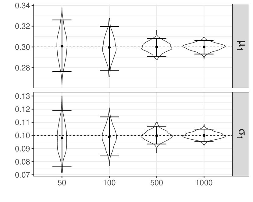
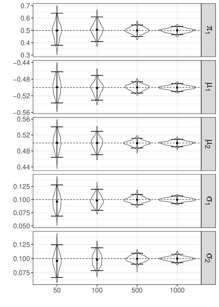
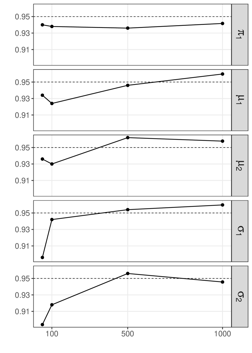
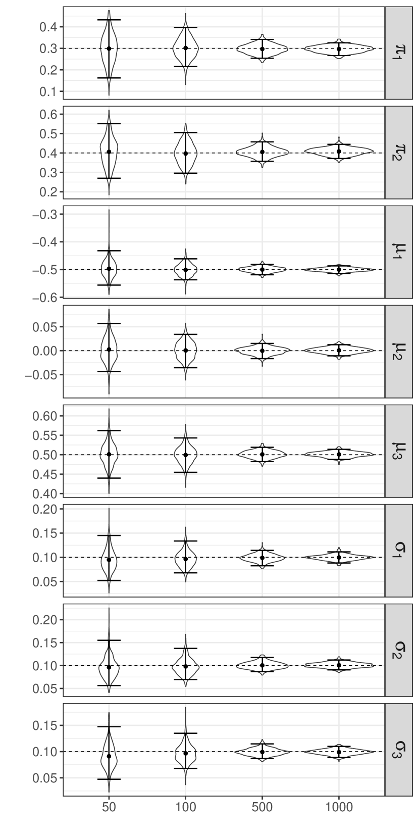
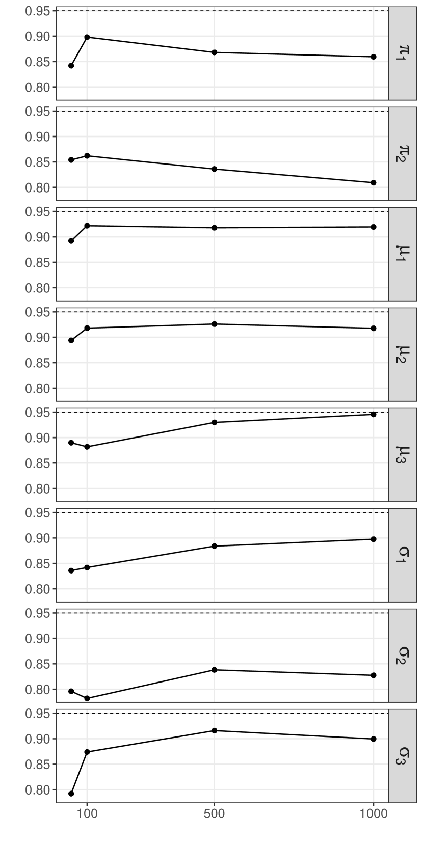
In our first simulation study, we generate simulated data from MR-Path under various parameter settings that mimic GWAS summary data used in practice. In each setting, we generate measurement errors as $\sigma_{X_{i}}^{2},\sigma_{Y_{i}}^{2}\sim\text{Inv. Gamma}(9,.0002)$. This is a reasonable choice as modern GWAS are conducted with large sample sizes which result in low measurement errors. Moreover, we set the instrument strength parameter to be $\lambda_{x}=10/\sqrt{p}$ to keep the norm constant across $p$. We vary the number of genetic variants to be $p=50,100,500,1000$ and the number of clusters to be $K_{\text{true}}=1,2,3$. In MR, we do not expect the number of clusters to be greater than 3 and the number of filtered genetic variants to be large. For each parameter setting, we ran the MC-EM algorithm with $K=K_{\text{true}}$ and computed the approximated confidence intervals with 500 simulated data-sets to obtain parameter estimates and 95% coverage probabilities. As the EM algorithm is sensitive to initial value specification, for each repetition, we ran the MC-EM algorithm 10 times with different random initial values and report the results from the run with the largest complete-data log likelihood. We perform a sensitivity analysis for the initial values in the MC-EM algorithm in appendix G. Simulation results are presented in figs. 5, 6 and 7. Note that as $K$ increases, we chose mixture means to be closer in value, making the estimation task more challenging.

In most scenarios, the parameter estimates obtained from the 500 replications are centered around the true value with the variance decreasing as a function of $p$. Furthermore, the coverage probabilities only deviate at most 5% from the desired 95% for $K=1,2$. However, the coverage probabilities for certain parameters are much lower than the desired level for $K=3$ even as $p$ increases. Since the parameter estimates are still centered around the true value, this phenomenon is likely due to underestimation of the standard error.

Figure 5: Simulation study results for $K=1$ ($\mu_{1}=0.3$, $\sigma_{1}=0.1$) with 500 replications. Left: Violin plots, 2.5% and 97.5% quantiles (solid horizontal line), mean (solid point) of parameter estimates as a function of the sample size $p$. Right: 95% coverage probabilities as a function of $p$ for each parameter.

Figure 6: Simulation study results for $K=2$ ($\pi_{1}=0.5$, $\mu_{1}=-0.5$, $\mu_{2}=0.5$, $\sigma_{1}=\sigma_{2}=0.1$) with 500 replications. Left: Violin plots, 2.5% and 97.5% quantiles (solid horizontal line), mean (solid point) of parameter estimates as a function of the sample size $p$. Right: 95% coverage probabilities as a function of $p$ for each parameter.

Figure 7: Simulation study results for $K=3$ ($\pi_{1}=\pi_{3}=0.3$, $\mu_{1}=-0.5$, $\mu_{2}=0$, $\mu_{3}=0.5$, $\sigma_{1}=\sigma_{2}=\sigma_{3}=0.1$) with 500 replications. Left: Violin plots, 2.5% and 97.5% quantiles (solid horizontal line), mean (solid point) of parameter estimates as a function of the sample size $p$. Right: 95% coverage probabilities as a function of $p$ for each parameter.

6.2 Model Selection with modified BIC

In our second simulation study, we simulate data from the MR-Path model with $p=50$ or $250$ and $\sqrt{p}\lambda_{x}=1$ or $5$. In each setting, we set the true number of clusters $K_{\text{true}}=1$,$2$, or $3$. In each replication, we ran the MC-EM algorithm with $K=1,2,3$ and chose the $K$ that yields the lowest modified BIC value. Results for this simulation study are shown in table 2.

Table 2: Results from second simulation study. For each setting, we simulated $N_{\text{rep}}=500$ data-sets. For $K_{\text{true}}=1$, we set $\mu_{1}=0.5$ and $\sigma_{1}=0.1$. For $K_{\text{true}}=2$, we set $\pi_{1}=0.5$, $\mu=(-0.5,0.5)$, and $\sigma_{1}=\sigma_{2}=0.1$. For $K_{\text{true}}=3$, we set $\pi_{1}=\pi_{2}=1/3$, $\mu=(-0.5,0,0.5)$, and $\sigma_{1}=\sigma_{2}=\sigma_{3}=0.05$. The last 3 columns report the proportion of replications for each setting where the modified BIC chose the corresponding $K_{\text{BIC}}$.

			Proportion
$p$	$\sqrt{p}\lambda_{x}$	$K_{\text{true}}$	$K_{\text{BIC}}=1$	$K_{\text{BIC}}=2$	$K_{\text{BIC}}=3$
50	1	1	.84	.06	.1
		2	0	.83	.17
		3	0	.03	.97
	5	1	.98	.01	.01
		2	0	.95	.05
		3	0	.01	.99
250	1	1	.91	.05	.04
		2	0	.91	.09
		3	.04	.03	.93
	5	1	1	0	0
		2	0	1	0
		3	0	0	1

From table 2, we observe that lower values for $\sqrt{p}\lambda_{x}$ result in the largest decreases in the accuracy of the modified BIC. For example, when $p=50$ and $K_{\text{true}}=2$, the modified BIC chose the correct $K$ 95% of the time when $\sqrt{p}\lambda_{x}=5$ but only 83% of the time when $\sqrt{p}\lambda_{x}=1$. We also notice that when $\sqrt{p}\lambda_{x}=1$, the accuracy of the modified BIC decreases with $p$. A practical consequence of this observation is that the modified BIC is more likely to choose the correct $K$ with few strong instruments than with more weak instruments.

Furthermore, we simulated addditional data from the MR-Path model with $K_{\text{true}}=1$, $\sqrt{p}\lambda_{x}=1,5$ and $\sigma=1,5,10$ to assess how well the modified BIC is able to correctly identify the true number of clusters as cluster variance increases. The results for these simulations are given in table 3.

To our surprise, the modified BIC criterion is more accurate as the true cluster variance increases. From table 3, we can see that for $K_{\text{true}}=1$, $p=50$, and $\sqrt{p}\lambda_{x}=1$, the modified BIC criterion chose the correct number of clusters only 84% of the time when $\sigma_{1}=0.1$, whereas it chose correctly 98.8% of the time when $\sigma_{1}=1$. However, the estimates of $\mu_{1}$ across replications where the BIC criterion chooses $K=1$ have a mean further away from the true value $0.5$ and a larger standard deviation as $\sigma_{1}$ increases.

Table 3: Results from simulation study to assess performance of BIC criterion when clusters have high variance. For each setting, we simulated $N_{\text{rep}}=500$ data sets with $K_{\text{true}}=1$ and $\mu_{1}=0.5$. The first three columns display the simulation parameters used in each setting. The next three columns report the proportion of replications for each setting where the modified BIC chose the corresponding $K_{\text{BIC}}$. The last three columns report the mean and standard deviation of the estimated cluster mean $\hat{\mu}_{1}$ across replications in each setting.

			Proportion			$\hat{\mu}_{1}$ when $K_{\text{BIC}}=1$
$p$	$\sqrt{p}\lambda_{x}$	$\sigma_{1}$	$K_{\text{BIC}}=1$	$K_{\text{BIC}}=2$	$K_{\text{BIC}}=3$	Mean	Std. Dev.
50	1	0.1	.840	.062	.098	.500	.017
		1	.988	.010	.002	.508	.132
		5	.992	.006	.002	.538	.654
		10	.992	.008	0	.621	1.300
	5	0.1	.975	.014	.011	.501	.013
		1	.991	.009	0	.509	.131
		5	.995	.005	0	.552	.665
		10	.997	.003	0	.619	1.330
250	1	0.1	.910	.053	.037	.497	.010
		1	.996	0	.004	.499	.069
		5	1	0	0	.505	.336
		10	1	0	0	.566	.694
	5	0.1	1	0	0	.500	.007
		1	1	0	0	.503	.066
		5	1	0	0	.517	.328
		10	1	0	0	.539	.658

7 Real data applications

7.1 Results for the motivating HDL-CHD example

We now return to the motivating example introduced in Section 1.1. The dataset being used is created from several large-scale GWAS datasets for plasma lipids (HDL-C, LDL-C, triglycerides) (Teslovich et al., 2010; Willer et al., 2013), coronary heart disease (Nikpay et al., 2015), lipoprotein subfractions (Kettunen et al., 2016), and other cardiovascular diseases. We use the three-sample summary-data MR design described in Zhao et al. (2020) to preprocess and homogenize the datasets. We first select 151 independent SNPs (distance $\geq$ 10 mega base pairs, $R^{2}\leq 0.001$ in a reference panel) that are associated with at least one plasma lipid trait (defined as the minimum $p$-value with HDL-C, LDL-C, and triglycerides less than $10^{-4}$). We then obtain the GWAS associations of these SNPS with all the other cardiometabolic traits. For the purpose of this example, we will focus on 31 SNPs that showed genome-wide significant associations ($p$-value $\leq 5\times 10^{-8}$) with HDL-C in the selection GWAS.

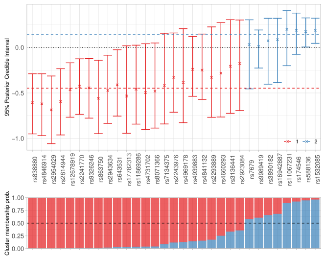
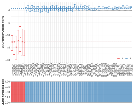
We apply the Monte Carlo EM algorithm developed in Section 5 to the 31 genetic instruments and their associations with HDL-C in a separate dataset (Kettunen et al., 2016) and CHD. The modified BIC from section 5.5 for $K=1$ and $K=2$ was -384.72 and -385.54, respectively, which slightly favors $K=2$. In other words, the data supports a model with mechanistic heterogeneity. The larger cluster ($\hat{\pi}_{1}=0.82$) corresponds to a negative effect ($\hat{\mu}_{1}=-0.343$, $\hat{\sigma}_{1}=0.23$) and the smaller cluster ($\hat{\pi}_{2}=0.18$) corresponds to a positive effect ($\hat{\mu}_{2}=0.14$, $\hat{\sigma}_{2}=0.09$). The SNPs are classified into the two clusters based on their posterior probabilities (Section 5.4). Figure 1(b) shows the scatterplot of the HDL-CAD data with the MC-EM parameter estimates. Figure 8 shows the posterior estimates of the variant-specific $\beta_{j}$ along side the cluster membership probabilities.

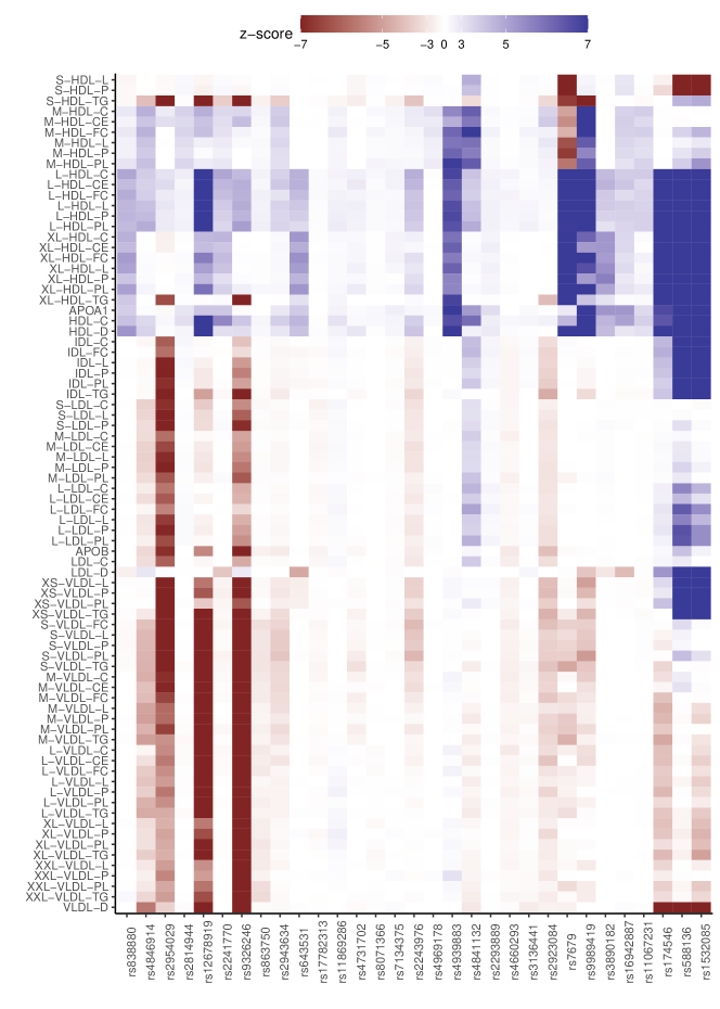
To validate the mechanistic heterogeneity identified by MR-Path, we generate a heatmap of the associations (z-scores) of the SNPs with lipoprotein subfraction traits (Kettunen et al., 2016). Most of the traits are named after their size (XS = extra small, S = small, M = medium, L = large, XL = extra large, XXL = double extra large), their lipoprotein class (HDL, IDL = intermediate-density lipoprotein, LDL, VLDL = very-low-density lipoprotein), and the measurement (C = total cholesterol, CE = cholesterol esters, FC = free cholesterol, L = total lipid, P = particle concentration, PL = phosolipids, TG = triglycerides). Other traits including the mean diameter of HDL/LDL/VLDL particles (HDL-D/LDL-D/VLDL-D) and the concentration of ApoA1/ApoB (major protein component of HDL/LDL). To aid visualization, the SNPs are ordered by their cluster membership probabilities and the lipoprotein subfractions are ordered by their density and size.

The heatmap in Figure 9 shows that the SNP clusters found by the mixture model exhibit different patterns of association with the lipoprotein subfractions. Several SNPs in the first cluster have strong inverse association with LDL-C and other LDL/VLDL subfraction traits. Therefore, the negative effect of HDL-C on CHD suggested by the instruments in the first cluster cluster may indeed be due to their pleiotropic effect on LDL-C and ApoB-containing lipoproteins (see scenario 1 in Figure 3(a)). In contrast, several SNPs in the second cluster (rs1532085, rs588136, rs174546, rs7679) are inversely associated with the concentration of small HDL particles, so they may be related to another mechanism that regulates the size of HDL particles. Although the instruments in this cluster suggest a positive effect of HDL-C on CHD, this may be explained by heterogeneous effects of cholesterol contained in different HDL subfractions (see scenario 2 in Figure 3(a)). An earlier univariable MR study indeed found that the concentration of small and medium HDL particles may have a negative effect on CHD, while the large and extra large HDL particles seem to have no effect (Zhao et al., 2019). To summarize, the heatmap provides some evidence that the clustering structure identified by our mixture model indeed corresponds to some distinct underlying mechanisms.

Figure 8: SNP-specific posterior quantities in HDL-CAD data. The SNPs are ordered by their posterior probability of belonging to cluster 2. Top: 95% posterior credible intervals. Colored dashed lines are the estimated cluster means and x-marks are the posterior medians for each SNP. Bottom: Posterior cluster membership probabilities bar plot. Vertical axis is posterior probability of belonging to cluster 2.

Figure 9: A heatmap showing the z-scores of the SNPs’ associations with lipoprotein subfraction measurements. The SNPs are ordered by their posterior probability of belonging to cluster 2 as in Figure 8. The lipoprotein subfractions are ordered by their density and size.

7.2 The role of adiposity in type II diabetes

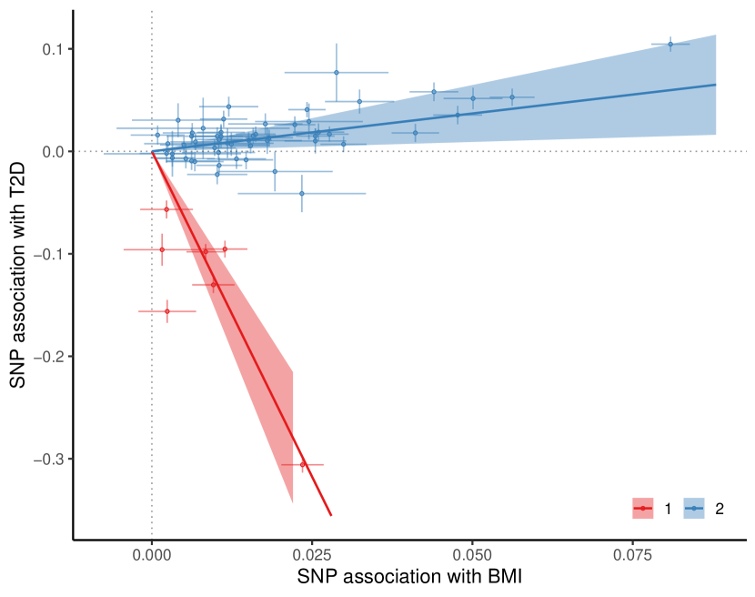
We now turn to a second example to illustrate the utility of MR-Path. In this example, we are interested in possible mechanistic heterogeneity of the effect of adiposity (as measured by the body mass index, BMI) on type II diabetes (T2D). Following the same three-sample summary-data MR design as described in Section 7.1, we created a dataset of 60 SNPs from two GWAS summary datasets for BMI (Akiyama et al., 2017; Locke et al., 2015) and one for T2D (Mahajan et al., 2018). We then apply the Monte Carlo EM algorithm developed in Section 5. The modified BIC selects $K=2$ clusters of SNPs. The larger cluster ($\hat{\pi}_{2}=0.88$) corresponds to a positive effect ($\hat{\mu}_{1}=0.77$, $\hat{\sigma}_{2}=0.42$) and the smaller cluster ($\hat{\pi}_{1}=0.12$) corresponds to a very large negative effect ($\hat{\mu}_{1}=-12.4$, $\hat{\sigma}_{1}=1.8$). See Figure 10(b) for a scatterplot of the data with effect estimates from MR-Path.

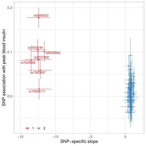
We did a GWAS catalog (Buniello et al., 2019) search for the SNPs belonging to cluster 2 and found that several of them are related to insulin function which tightly regulates glucose level and plays a crucial role in diabetes. This motivated us to compare the estimate variant-specific effect $\hat{\beta}_{i}$ with the SNP association with peak blood insulin, which is available from an independent GWAS (Wood et al., 2017) (Figure 12). In fact, six out of the seven SNPs classified into cluster 2 are strongly associated with peak blood insulin. This shows that the large negative effect of this cluster is most likely due to horizontal pleiotropy (Figure 3(a)) instead of a genuine negative causal effect of adiposity. The results we obatined here are broadly consistent with other recent genetic studies that have identified SNPs with opposite effects on adiposity and type II diabetes and linked the “favorable adiposity” genes to insulin function and fat distribution (Ji et al., 2019).

(a) MR-RAPS & MR-Egger

(b) MR-Path

Figure 10: Scatterplot of BMI-T2D data and effect estimates. Left: Line/shaded region represents the causal effect estimate $\pm$ one standard error from MR-RAPS and MR-Egger. Right: Lines/shaded regions represent heterogeneous causal effect estimates $\pm$ one standard deviation from MR-Path.

Figure 11: SNP-specific posterior quantities in BMI-T2D data. SNPs are ordered by their posterior probability of belonging to cluster 2. Top: 95% posterior credible intervals. Colored dashed lines are the estimated cluster means (same as Figure 10) and x-marks are the posterior medians for each SNP. Bottom: Posterior cluster membership probabilities bar plot. Vertical axis is posterior probability of belonging to cluster 2.

Figure 12: Relationship of SNP-specific slope and the association with peak blood insulin. The horizontal axis is the posterior median of the SNP-specific slope $\beta_{i}$ with standard error bars. The vertical axis is the SNP association with peak blood insulin with standard error bars reported in an independent GWAS. The SNPs are colored according to the cluster with the highest posterior cluster membership probability $P(\xi_{i}=k|\hat{\theta}_{X_{i}},\hat{\theta}_{Y_{i}})$.

8 Discussion

In this paper, we have formalized the notion of mechanistic heterogeneity in the context of MR and showed that SNPs on the same biological pathway identify similar causal effects. Different pathways generally correspond to different causal effects, even if they are all valid instruments. Motivated by this observation, we introduced MR-Path, an interpretable mixture model for summary-level GWAS data that can provide valuable insights on mechanistic heterogeneity.

A conclusion of mechanistic heterogeneity can be used in several ways. If we are in scenario 1 shown in fig. 3(a), where heterogeneity is caused by multiple pathways of horizontal pleiotropy, we can try to identify mediating exposures for pleiotropic mechanisms and then use a multivariable MR method to effectively remove the heterogeneity caused by horizontal pleiotropy. For scenario 2 shown in fig. 3(b), where there are multiple mechanisms for the exposure, genetic enrichment analysis could be helpful in identifying the upstream pathways. Both cases rely on post-hoc analyses with external data which is beyond the scope of this paper. Nevertheless, we illustrated some possibilities in our two real data applications in section 7.

MR-Path has several advantages over similar existing methods for MR. First, it relaxes the effect homogeneity assumption implicit in most existing MR methods so it is able to identify multiple causal mechanisms. Second, MR-Path does not require substantial domain knowledge since we use a data-driven approach to select the number of clusters. However, this means that MR-Path is not able to distinguish between the different mechanisms in fig. 3 without further post-hoc analysis (Wang et al. (2020)). Lastly, MR-Path is based on a full likelihood and is robust to weak instrument bias since we use an error-in-variables approach to estimate the variant-specific causal effects.

We showed using numerical simulations that our MC-EM algorithm gives parameter estimates that are close to the ground truth and the corresponding approximate confidence intervals have coverage probabilities close to their true values. We also showed that the modified BIC criterion we used for selecting the number of clusters chose correctly a majority of the time.

We demonstrated the utility of MR-Path in modeling mechanistic heterogeneity in MR analysis by using it to investigate the causal mechanisms between HDL-C and CHD and between adioposity and type II diabetes. These examples reinforce the importance of considering multiple causal mechanisms in MR analysis. Our findings are consistent with existing genetic studies that use external data. For the HDL-C and CHD data set, MR-Path identifies a cluster with a positive average causal effect which may be associated with a mechanism that regulates size of HDL particles. In our study of the role of adioposity on type II diabetes, MR-Path finds a cluster with a negative average causal effect that is likely attributed to horizontal pleiotropy.

Since MR-Path is a generative model for multiple causal mechanisms in MR, there are many potential extensions that can be incorporated in future work. One such extension is to replace our univariate mixture model with a multivariate model to consider multiple risk exposures simultaneously. The multivariate version of MR-Path can be used to account for the pleiotropic effects of other lipoproteins in our HDL and CHD example. Another possible extension is to allow for correlated SNPs by relaxing the independence assumption in assumption 4.1.

Appendix A Derivation of $P(\beta_{i}|\theta_{X_{i}},\hat{\theta}_{Y_{i}},\varphi)$

In this section, we will derive eq. 12 by first deriving $P(\beta_{i}|\xi_{i}=k,\theta_{X_{i}},\hat{\theta}_{Y_{i}},\varphi)$ and $\tilde{\pi}_{ik}:=P(\xi_{i}=k|\theta_{X_{i}},\hat{\theta}_{Y_{i}},\varphi)$, for $k=1,\dots,K$. Then, $P(\beta_{i}|\theta_{X_{i}},\hat{\theta}_{Y_{i}},\varphi)=\sum_{k=1}^{K}\tilde{\pi}_{ik}P(\beta_{i}|\xi_{i}=k,\theta_{X_{i}},\hat{\theta}_{Y_{i}},\varphi)$. For notational convenience, we will drop the dependence on model parameters $\varphi$.

$$P(\beta_{i}|\xi_{i}=k,\theta_{X_{i}},\hat{\theta}_{Y_{i}}) \propto P(\hat{\theta}_{Y_{i}}|\theta_{X_{i}},\beta_{i})P(\beta_{i}|\xi_{i}=k)$$

$$\propto\exp\Big{\{}-\frac{1}{2}\Big{[}\sigma_{Y_{i}}^{-2}(\hat{\theta}_{Y_{i}}-\beta_{i}\theta_{X_{i}})^{2}+\sigma_{k}^{-2}(\beta_{i}-\mu_{k})^{2}\Big{]}\Big{\}}$$

$$\propto\exp\Big{\{}(\sigma_{Y_{i}}^{-2}\theta_{X_{i}}^{2}+\sigma_{k}^{-2})\beta_{i}^{2}-2(\sigma_{Y_{i}}^{-2}\theta_{X_{i}}\hat{\theta}_{Y_{i}}+\sigma_{k}^{-2}\mu_{k})\beta_{i}\Big{\}}.$$ (25)

It follows from completing the square that $\beta_{i}|\xi_{i}=k,\theta_{X_{i}},\hat{\theta}_{Y_{i}}\sim N(\tilde{\mu}_{ik},\tilde{\sigma}_{ik}^{2})$, where $\tilde{\mu}_{ik}$ and $\tilde{\sigma}_{ik}^{2}$ are given in eq. 13.

$$P(\xi_{i}=k|\theta_{X_{i}},\hat{\theta}_{Y_{i}}) \propto P(\xi_{i}=k)P(\hat{\theta}_{Y_{i}}|\xi_{i}=k,\theta_{X_{i}})$$

$$\propto\pi_{k}\int P(\hat{\theta}_{Y_{i}}|\theta_{X_{i}},\beta_{i})P(\beta_{i}|\xi_{i}=k)d\beta_{i}.$$

From eq. 25, we have that $\int P(\hat{\theta}_{Y_{i}}|\theta_{X_{i}},\beta_{i})P(\beta_{i}|\xi_{i}=k)d\beta_{i}=\Big{[}(\sigma_{Y_{i}}^{-2}\theta_{X_{i}}^{2}+\sigma_{k}^{-2})\Big{]}^{1/2}$. Then, $P(\xi_{i}=k|\theta_{X_{i}},\hat{\theta}_{Y_{i}})=\tilde{\pi}_{ik}$.

Appendix B Bounded Importance Sampling Weights

Following eq. 14, the importance weights are given by

$$w_{i}^{j} =\frac{P(\theta_{X_{i}}|\hat{\theta}_{X_{i}},\hat{\theta}_{Y_{i}},\varphi)}{P(\theta_{X_{i}}|\hat{\theta}_{X_{i}},\varphi)}$$

$$\propto P(\theta_{X_{i}}|\hat{\theta}_{X_{i}},\varphi)P(\hat{\theta}_{Y_{i}}|\theta_{X_{i}},\varphi)$$

$$=\sum_{k=1}^{K}\frac{\pi_{k}}{\sqrt{2\pi\theta_{X_{i}}^{2}\sigma_{k}^{2}+\sigma_{Y_{i}}^{2}}}\exp\Big{\{}-\frac{1}{2(\theta_{X_{i}}^{2}\sigma_{k}^{2}+\sigma_{Y_{i}}^{2})}(Y_{i}-\theta_{X_{i}}\mu_{k})^{2}\Big{\}}\leq\frac{1}{\sqrt{2\pi\sigma_{Y_{i}}^{2}}},$$

for $i=1,\dots,p;j=1,\dots,M$. Therefore, the importance weights are bounded and have a finite variance.

Appendix C Importance sampling estimate of $\eta^{2}$

An importance sampling estimate of $\eta^{2}$ at iteration $t$ in eq. 23 is given by

$$\hat{\eta}^{2}=m_{t}\sum_{i=1}^{p}\Big{\{}\sum_{j=1}^{m_{t}}w_{i}^{j}\Lambda_{ij}^{(t)}\Big{\}}^{2}\Big{[}\frac{\sum_{j=1}^{m_{t}}(w_{i}^{j}\Lambda_{ij}^{(t)})^{2}}{(\sum_{j=1}^{m_{t}}w_{i}^{j}\Lambda_{ij}^{(t)})^{2}}-2\frac{\sum_{j=1}^{m_{t}}(w_{i}^{j})^{2}\Lambda_{ij}^{(t)}}{\sum_{j=1}^{m_{t}}w_{i}^{j}\Lambda_{ij}^{(t)}}+\sum_{j=1}^{m_{t}}(w_{i}^{j})^{2}\Big{]},$$

where $\Lambda_{ij}^{(t)}$ is given in eq. 22.

Appendix D Comparison with MR-Clust

In this section, we will compare MR-Path with a similar method for identifying heterogeneity in Mendelian Randomization known as MR-Clust (Foley, Kirk and Burgess (2019)). A fundamental difference between MR-Path and MR-Clust is that the former assumes an error-in-variables regression model for the observed instrument-exposure and instrument-outcome associations (assumption 4.1) and models variant-specific causal effects as a latent variable that follows a mixture distribution, while the latter models the Wald ratio estimates $\hat{\theta}_{i}=\hat{\theta}_{Y_{i}}/\hat{\theta}_{X_{i}}$ using a mixture model. More specifically, MR-Clust makes the following assumption:

$$\hat{\theta}_{i}|\{\Theta,\hat{\sigma}_{i}^{2},\xi_{i}=k\}\sim N(\mu_{k},\hat{\sigma}_{i}^{2}),\ \text{for }k=1,\dots,K,$$ (26)

where $\hat{\sigma}_{j}$ is the standard error of the $j$th ratio estimate and $\Theta$ is a vector of cluster means. Furthermore, MR-Clust assumes there are $K+2$ clusters of genetic variants, with $K$ substantive clusters, a null cluster, and a junk cluster. The null cluster is assumed to have mean $\mu_{0}=0$. The junk cluster follows a generalized t-distribution in order to account for the remaining genetic variants that do not belong to any other cluster. Similar to MR-Path, MR-Clust determines the number of clusters $K$ using the Bayesian information criterion (BIC).

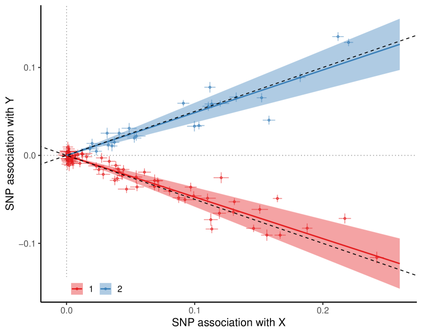
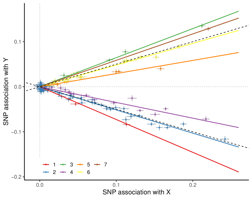
A downside of directly modeling ratio estimates is that they can be heavily biased for weak instruments (Zhao et al. (2020)), increasing the risk of detecting spurious clusters. By using an errors-in-variables regression approach, MR-Path is more robust to this weak instrument bias. To illustrate this, we simulated data from the model described in section 4 with $p=100$, $\theta_{X_{i}}\sim 0.7N(0,0.1)+0.3N(0,0.000001)$, $\pi=(0.6,0.4)$, $\mu=(-0.5,0.5)$, and $\sigma=(0.1,0.1)$. The estimates from MR-Path and MR-Clust are plotted in fig. 13. MR-Path chooses $K=2$ (by varying $K$ from 1 to 7 and picking the one with lowest modified BIC), while MR-Clust chooses $K=7$ using a similar model selection procedure. Another advantage of MR-Path over MR-Clust is that it constructs confidence intervals for the cluster means.

(a) MR-Path

(b) MR-Clust

Figure 13: Scatterplot of simulated data with many weak instruments and effect estimates from MR-Path (left) and MR-Clust (right). The dashed black line shows the true cluster means $(-0.5,0.5)$.

However, MR-Clust is more computationally efficient since the parameters in eq. 26 can be estimated using an exact EM algorithm. There are several ways to close this gap in computational efficiency that we will explore in future work. One possibility is to replace the MC-EM algorithm with a variational EM algorithm (Blei, Kucukelbir and Mcauliffe (2017)). However, finding a suitable variational approximation to the E-step may be challenging.

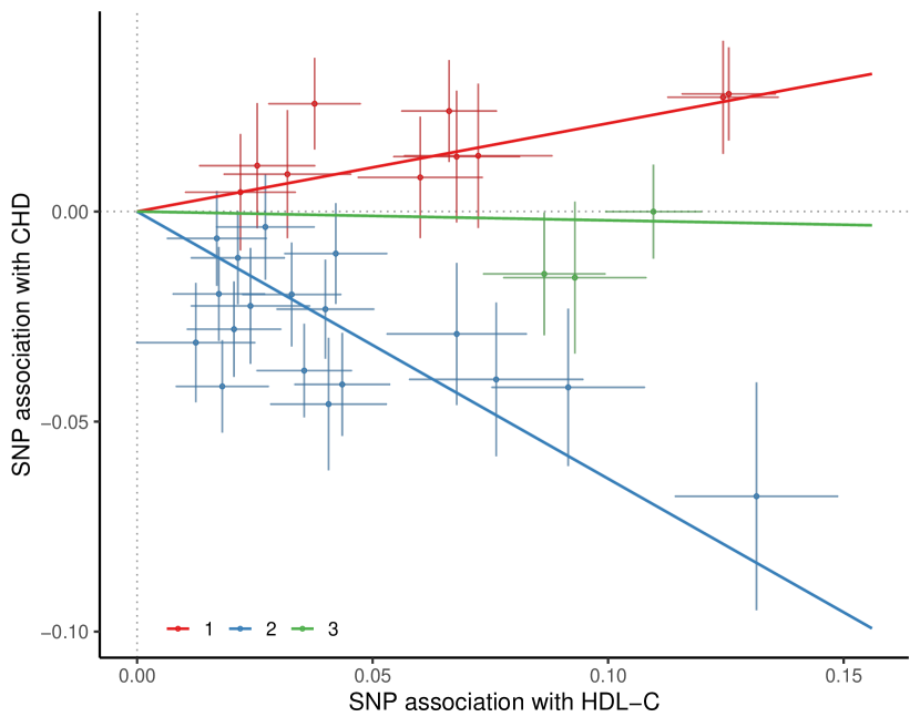
The results from MR-Path and MR-Clust applied to the motivating HDL-CAD data are plotted in fig. 14. In this case, MR-Clust detects two substantive clusters with means $0.21$ and $-0.64$ and one null cluster with mean $-0.021$. The two substantive clusters are similar to the two clusters detected by MR-Path.

(a) MR-Path

(b) MR-Clust

Figure 14: Scatterplot of HDL-CAD data similar to fig. 1 showing results from MR-Path (left) vs. MR-Clust (right). The 3rd cluster (green) from MR-Clust is the null cluster.

Appendix E Robustness of MR-Path under pleiotropy

To assess the robustness of MR-Path under pleiotropy, we simulate data from the model below and conduct a study similar to the one in section 6.1.

$$P(\beta_{i}=\mu_{k}) =\pi_{k},\ k=1,\dots,K,$$

$$\theta_{X_{i}} \sim N(0,\lambda_{x}^{2}),$$

$$\begin{pmatrix}\hat{\theta}_{X_{i}}\\ \hat{\theta}_{Y_{i}}\end{pmatrix}\Big{|}\ \theta_{X_{i}},\beta_{i},\alpha_{i} \sim N\Big{(}\begin{pmatrix}\theta_{X_{i}}\\ \alpha_{i}+\beta_{i}\theta_{X_{i}}\end{pmatrix},\begin{pmatrix}\sigma_{X_{i}}^{2}&0\\ 0&\sigma_{Y_{i}}^{2}\end{pmatrix}\Big{)},$$

where $\alpha_{i}$ represent the direct effect of SNP $i$ on the outcome. Similar to Zhao et al. (2020), we generate $\alpha_{i}$ in three different ways:

1. Normal: $\alpha_{i}\sim N(0,\tau_{0}^{2})$.

2. Laplace: $\alpha_{i}\sim\tau_{0}\cdot\text{Lap}(1)$, where $\text{Lap}(1)$ is the Laplace (double exponential) distribution with rate $1$.

3. Idiosyncratic: $\alpha_{i}$ is generated according to setup 1 above, except that for 10% of randomly selected SNPs, $\alpha_{i}\sim N(5\cdot\tau_{0},\tau_{0}^{2})$.

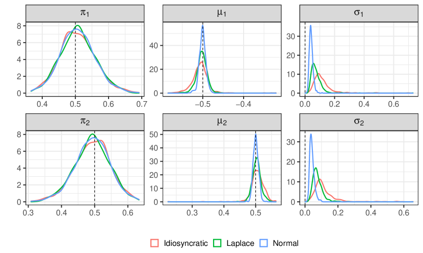
In each of the scenarios above, we set $\tau_{0}=(2/p)\sum_{j=1}^{p}\sigma_{Y_{i}}$. We generate measurements errors $\sigma_{X_{i}}^{2}$ and $\sigma_{Y_{i}}^{2}$ from the same distribution in section 6.1 and set $p=100$, $\lambda_{x}=10/\sqrt{p}$. Furthermore, we set $K=2$, where $\pi_{1}=0.5$, $\mu_{1}=-0.5$, and $\mu_{2}=0.5$. Density plots for the parameter estimates across 500 replications under each scenario above are shown in fig. 15. For each scenario, the estimates of $\pi_{1}$, $\mu_{1}$, and $\mu_{2}$ across replications are centered around the true value with increasing variance as we go from normally distributed $\alpha_{i}$ to idiosyncratic $\alpha_{i}$. This suggests that our proposed method is robust to different types of pleiotropy.

Figure 15: Density plots for MR-Path estimates of each parameter under different scenarios of pleiotropy.

Appendix F Computational efficiency of Monte-Carlo EM algorithm

For the HDL-CHD example in section 7.1, the MC-EM algorithm, including initial value optimization and model selection, took approximately 6 seconds to run on a Dell XPS-15 laptop with an Intel Core i7-8750H processor and 16GB of RAM. However, the MC-EM algorithm took roughly 2 minutes to run for the BMI-T2D example in section 7.2. This is because the algorithm converged much quicker for the HDL-CHD example. The BMI-T2D example required an average of 43 iterations and 80,000 Monte-Carlo samples at termination for each repetition, while the HDL-CHD example only required an average of 20 iterations and 5800 Monte-Carlo samples at termination. The computational bottleneck of the MC-EM algorithm is its memory usage since it requires saving a large matrix of importance samples in the E-step which grows in size with each iteration.

Appendix G Sensitivity Analysis for Monte-Carlo EM algorithm

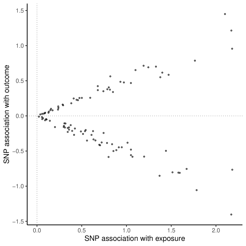
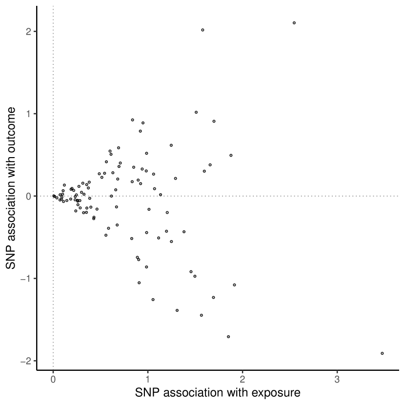
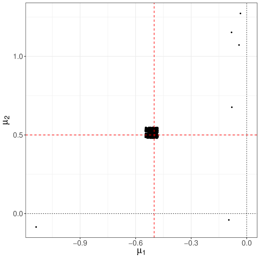
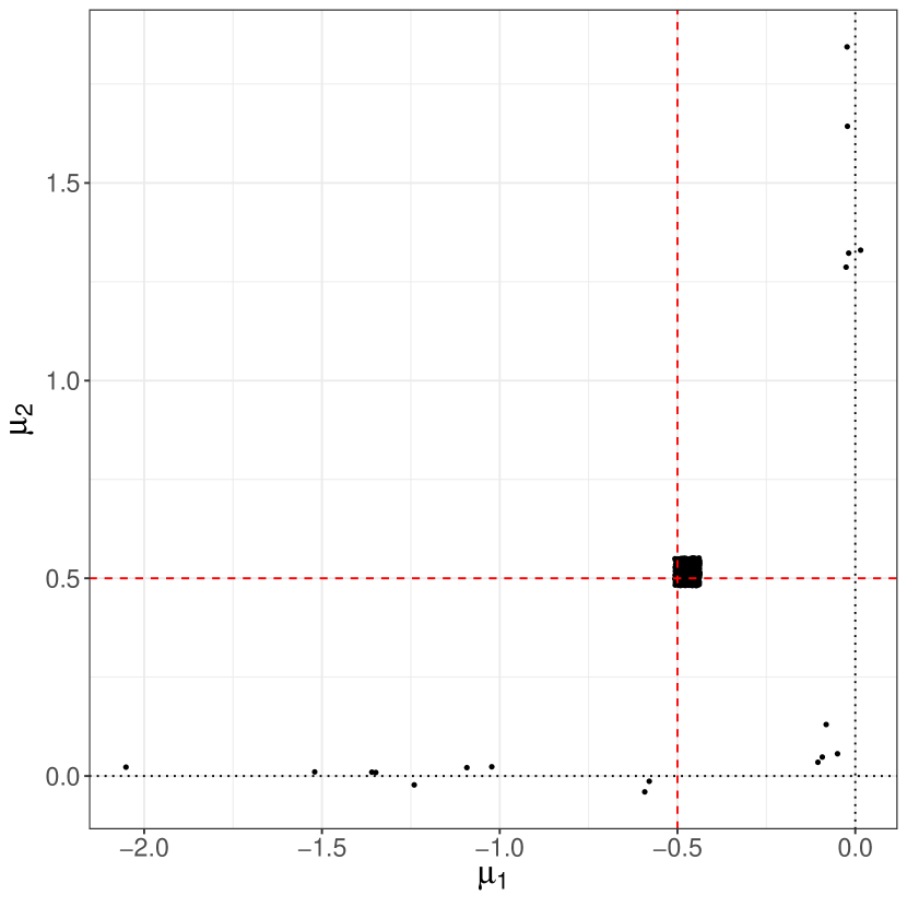
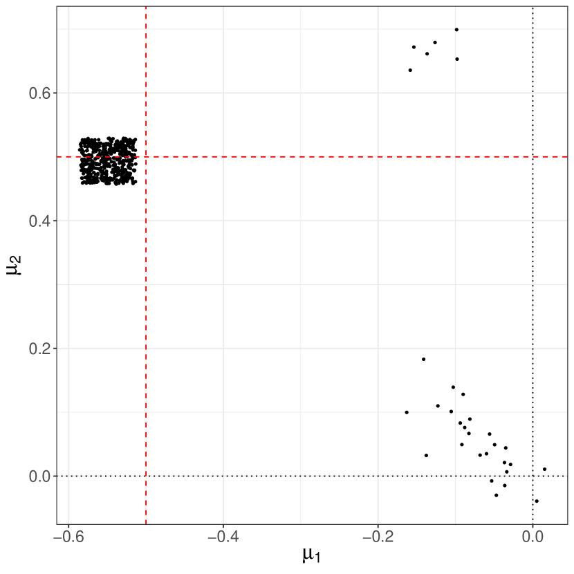
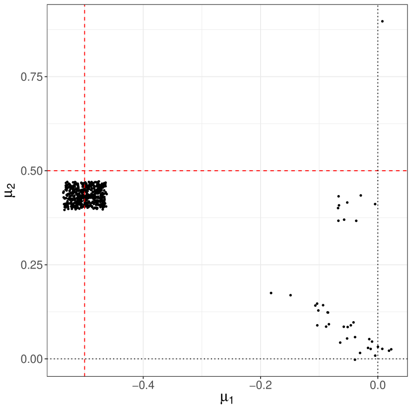
It is well known that the vanilla EM algorithm for Gaussian mixture models is sensitive to the initial values, especially when clusters overlap (Biernacki, Celeux and Govaert (2003); Shireman, Steinley and Brusco (2017)). In this section, we conduct a small-scale simulation study to evaluate how sensitive our proposed MC-EM algorithm is to initial values. In this simulation study, we set $K=2$, $\pi_{1}=\pi_{2}$, $\mu=(-0.5,0.5)$. We vary the instrument strength by setting $\sqrt{p}\lambda_{x}=5\text{ or }10$ and the degree to which clusters overlap by setting $\sigma_{1}=\sigma_{2}$ to be either $0.1$ (low overlap) or $0.3$ (high overlap). We simulate data from our proposed model with these parameters (shown in fig. 16) and apply the MC-EM algorithm with 500 different starting values. We plot the resulting $\mu$ estimates in fig. 17. These preliminary results suggest that the MC-EM algorithm becomes more sensitive to starting values as the degree of cluster overlap increases. In the cases where $\sigma_{1}=\sigma_{2}=0.1$, most of the estimates are close to the true values with a few estimates deviating from it. However, when $\sigma_{1}=\sigma_{2}=0.3$, most of the estimates are slightly biased from the truth with a small cluster of estimates close to the origin.

(a) Low overlap

(b) High overlap

Figure 16: Scatterplot of simulated data for sensitivity analysis.

(a) $\sqrt{p}\lambda_{x}=10$, $\sigma_{1}=\sigma_{2}=0.1$

(b) $\sqrt{p}\lambda_{x}=5$, $\sigma_{1}=\sigma_{2}=0.1$

(c) $\sqrt{p}\lambda_{x}=10$, $\sigma_{1}=\sigma_{2}=0.3$

(d) $\sqrt{p}\lambda_{x}=5$, $\sigma_{1}=\sigma_{2}=0.3$

Figure 17: Scatterplots of $\mu$ estimates from fitting MR-Path with 500 differrent starting values on simulated data with different $\sqrt{p}\lambda_{x}$ (columns) and $\sigma_{1}=\sigma_{2}$ (rows). True values of $\mu_{1}$ and $\mu_{2}$ are shown as red dashed lines.

[Acknowledgments] We would like to thank Xuelu Wang for helpful comments on the type II diabetes example.

References

- Akiyama et al. (2017) {barticle}[author] \bauthor\bsnmAkiyama, \bfnmMasato\binitsM., \bauthor\bsnmOkada, \bfnmYukinori\binitsY., \bauthor\bsnmKanai, \bfnmMasahiro\binitsM., \bauthor\bsnmTakahashi, \bfnmAtsushi\binitsA., \bauthor\bsnmMomozawa, \bfnmYukihide\binitsY., \bauthor\bsnmIkeda, \bfnmMasashi\binitsM., \bauthor\bsnmIwata, \bfnmNakao\binitsN., \bauthor\bsnmIkegawa, \bfnmShiro\binitsS., \bauthor\bsnmHirata, \bfnmMakoto\binitsM., \bauthor\bsnmMatsuda, \bfnmKoichi\binitsK. \betalet al. (\byear2017). \btitleGenome-wide association study identifies 112 new loci for body mass index in the Japanese population. \bjournalNature Genetics \bvolume49 \bpages1458. \endbibitem
- Anderson and Rubin (1949) {barticle}[author] \bauthor\bsnmAnderson, \bfnmTheodore W\binitsT. W. and \bauthor\bsnmRubin, \bfnmHerman\binitsH. (\byear1949). \btitleEstimation of the parameters of a single equation in a complete system of stochastic equations. \bjournalAnnals of Mathematical Statistics \bvolume20 \bpages46–63. \endbibitem
- Angrist, Imbens and Rubin (1996) {barticle}[author] \bauthor\bsnmAngrist, \bfnmJoshua D\binitsJ. D., \bauthor\bsnmImbens, \bfnmGuido W\binitsG. W. and \bauthor\bsnmRubin, \bfnmDonald B\binitsD. B. (\byear1996). \btitleIdentification of causal effects using instrumental variables. \bjournalJournal of the American Statistical Association \bvolume91 \bpages444–455. \endbibitem
- Armitage, Holmes and Preiss (2019) {barticle}[author] \bauthor\bsnmArmitage, \bfnmJane\binitsJ., \bauthor\bsnmHolmes, \bfnmMichael V\binitsM. V. and \bauthor\bsnmPreiss, \bfnmDavid\binitsD. (\byear2019). \btitleCholesteryl ester transfer protein inhibition for preventing cardiovascular events: JACC review topic of the week. \bjournalJournal of the American College of Cardiology \bvolume73 \bpages477–487. \endbibitem
- Biernacki, Celeux and Govaert (2003) {barticle}[author] \bauthor\bsnmBiernacki, \bfnmChristophe\binitsC., \bauthor\bsnmCeleux, \bfnmGilles\binitsG. and \bauthor\bsnmGovaert, \bfnmGérard\binitsG. (\byear2003). \btitleChoosing Starting Values for the EM Algorithm for Getting the Highest Likelihood in Multivariate Gaussian Mixture Models. \bjournalComputational Statistics & Data Analysis \bvolume41 \bpages561–575. \bdoi10.1016/S0167-9473(02)00163-9 \endbibitem
- Bishop (2006) {bbook}[author] \bauthor\bsnmBishop, \bfnmChristopher M.\binitsC. M. (\byear2006). \btitlePattern Recognition and Machine Learning (Information Science and Statistics). \bpublisherSpringer-Verlag, \baddressBerlin, Heidelberg. \endbibitem
- Blei, Kucukelbir and Mcauliffe (2017) {barticle}[author] \bauthor\bsnmBlei, \bfnmDavid M\binitsD. M., \bauthor\bsnmKucukelbir, \bfnmAlp\binitsA. and \bauthor\bsnmMcauliffe, \bfnmJon D\binitsJ. D. (\byear2017). \btitleVariational Inference: A Review for Statisticians. \bjournalJournal of the American Statistical Association \bvolume112 \bpages859–877. \bdoi10.1080/01621459.2017.1285773 \endbibitem
- Bowden, Davey Smith and Burgess (2015) {barticle}[author] \bauthor\bsnmBowden, \bfnmJack\binitsJ., \bauthor\bsnmDavey Smith, \bfnmGeorge\binitsG. and \bauthor\bsnmBurgess, \bfnmStephen\binitsS. (\byear2015). \btitleMendelian randomization with invalid instruments: effect estimation and bias detection through Egger regression. \bjournalInternational Journal of Epidemiology \bvolume44 \bpages512–525. \endbibitem
- Bowden et al. (2017) {barticle}[author] \bauthor\bsnmBowden, \bfnmJack\binitsJ., \bauthor\bsnmDel Greco M, \bfnmFabiola\binitsF., \bauthor\bsnmMinelli, \bfnmCosetta\binitsC., \bauthor\bsnmDavey Smith, \bfnmGeorge\binitsG., \bauthor\bsnmSheehan, \bfnmNuala\binitsN. and \bauthor\bsnmThompson, \bfnmJohn\binitsJ. (\byear2017). \btitleA framework for the investigation of pleiotropy in two-sample summary data Mendelian randomization. \bjournalStatistics in Medicine \bvolume36 \bpages1783–1802. \endbibitem
- Boyle, Li and Pritchard (2017) {barticle}[author] \bauthor\bsnmBoyle, \bfnmEvan A\binitsE. A., \bauthor\bsnmLi, \bfnmYang I\binitsY. I. and \bauthor\bsnmPritchard, \bfnmJonathan K\binitsJ. K. (\byear2017). \btitleAn expanded view of complex traits: from polygenic to omnigenic. \bjournalCell \bvolume169 \bpages1177–1186. \endbibitem
- Buniello et al. (2019) {barticle}[author] \bauthor\bsnmBuniello, \bfnmAnnalisa\binitsA., \bauthor\bsnmMacArthur, \bfnmJacqueline A L\binitsJ. A. L., \bauthor\bsnmCerezo, \bfnmMaria\binitsM., \bauthor\bsnmHarris, \bfnmLaura W\binitsL. W., \bauthor\bsnmHayhurst, \bfnmJames\binitsJ., \bauthor\bsnmMalangone, \bfnmCinzia\binitsC., \bauthor\bsnmMcMahon, \bfnmAoife\binitsA., \bauthor\bsnmMorales, \bfnmJoannella\binitsJ., \bauthor\bsnmMountjoy, \bfnmEdward\binitsE., \bauthor\bsnmSollis, \bfnmElliot\binitsE. \betalet al. (\byear2019). \btitleThe NHGRI-EBI GWAS Catalog of published genome-wide association studies, targeted arrays and summary statistics 2019. \bjournalNucleic acids research \bvolume47 \bpagesD1005–D1012. \endbibitem
- Burgess, Butterworth and Thompson (2013) {barticle}[author] \bauthor\bsnmBurgess, \bfnmStephen\binitsS., \bauthor\bsnmButterworth, \bfnmAdam\binitsA. and \bauthor\bsnmThompson, \bfnmSimon G\binitsS. G. (\byear2013). \btitleMendelian randomization analysis with multiple genetic variants using summarized data. \bjournalGenetic Epidemiology \bvolume37 \bpages658–665. \bdoi10.1002/gepi.21758 \endbibitem
- Burgess et al. (2017) {barticle}[author] \bauthor\bsnmBurgess, \bfnmStephen\binitsS., \bauthor\bsnmBowden, \bfnmJack\binitsJ., \bauthor\bsnmFall, \bfnmTove\binitsT., \bauthor\bsnmIngelsson, \bfnmErik\binitsE. and \bauthor\bsnmThompson, \bfnmSimon G\binitsS. G. (\byear2017). \btitleSensitivity Analyses for Robust Causal Inference from Mendelian Randomization Analyses with Multiple Genetic Variants. \bjournalEpidemiology (Cambridge, Mass.) \bvolume28 \bpages30–42. \bdoi10.1097/EDE.0000000000000559 \endbibitem
- Burgess et al. (2020) {barticle}[author] \bauthor\bsnmBurgess, \bfnmStephen\binitsS., \bauthor\bsnmFoley, \bfnmChristopher N\binitsC. N., \bauthor\bsnmAllara, \bfnmElias\binitsE., \bauthor\bsnmStaley, \bfnmJames R\binitsJ. R. and \bauthor\bsnmHowson, \bfnmJoanna M M\binitsJ. M. M. (\byear2020). \btitleA robust and efficient method for Mendelian randomization with hundreds of genetic variants. \bjournalNature Communications \bvolume11 \bpages376. \bdoi10.1038/s41467-019-14156-4 \endbibitem
- Caffo, Jank and Jones (2005) {barticle}[author] \bauthor\bsnmCaffo, \bfnmBrian S\binitsB. S., \bauthor\bsnmJank, \bfnmWolfgang\binitsW. and \bauthor\bsnmJones, \bfnmGalin L\binitsG. L. (\byear2005). \btitleAscent-based Monte Carlo expectation– maximization. \bjournalJournal of the Royal Statistical Society: Series B (Statistical Methodology) \bvolume67 \bpages235–251. \bdoi10.1111/j.1467-9868.2005.00499.x \endbibitem
- Davey Smith and Phillips (2020) {barticle}[author] \bauthor\bsnmDavey Smith, \bfnmGeorge\binitsG. and \bauthor\bsnmPhillips, \bfnmAndrew N\binitsA. N. (\byear2020). \btitleCorrelation without a cause: an epidemiological odyssey. \bjournalInternational Journal of Epidemiology \bvolume49 \bpages4-14. \bdoi10.1093/ije/dyaa016 \endbibitem
- Didelez and Sheehan (2007) {barticle}[author] \bauthor\bsnmDidelez, \bfnmVanessa\binitsV. and \bauthor\bsnmSheehan, \bfnmNuala\binitsN. (\byear2007). \btitleMendelian randomization as an instrumental variable approach to causal inference. \bjournalStatistical Methods in Medical Research \bvolume16 \bpages309–330. \bdoi10.1177/0962280206077743 \endbibitem
- Foley, Kirk and Burgess (2019) {barticle}[author] \bauthor\bsnmFoley, \bfnmChristopher N\binitsC. N., \bauthor\bsnmKirk, \bfnmPaul DW\binitsP. D. and \bauthor\bsnmBurgess, \bfnmStephen\binitsS. (\byear2019). \btitleMR-Clust: Clustering of genetic variants in Mendelian randomization with similar causal estimates. \bjournalbioRxiv \bpages2019.12.18.881326. \bdoi10.1101/2019.12.18.881326 \endbibitem
- Ibrahim, Zhu and Tang (2008) {barticle}[author] \bauthor\bsnmIbrahim, \bfnmJoseph G\binitsJ. G., \bauthor\bsnmZhu, \bfnmHongtu\binitsH. and \bauthor\bsnmTang, \bfnmNiansheng\binitsN. (\byear2008). \btitleModel Selection Criteria for Missing-Data Problems Using the EM Algorithm. \bjournalJournal of the American Statistical Association \bvolume103 \bpages1648–1658. \bdoi10.1198/016214508000001057 \endbibitem
- Ji et al. (2019) {barticle}[author] \bauthor\bsnmJi, \bfnmYingjie\binitsY., \bauthor\bsnmYiorkas, \bfnmAndrianos M\binitsA. M., \bauthor\bsnmFrau, \bfnmFrancesca\binitsF., \bauthor\bsnmMook-Kanamori, \bfnmDennis\binitsD., \bauthor\bsnmStaiger, \bfnmHarald\binitsH., \bauthor\bsnmThomas, \bfnmE Louise\binitsE. L., \bauthor\bsnmAtabaki-Pasdar, \bfnmNaeimeh\binitsN., \bauthor\bsnmCampbell, \bfnmArchie\binitsA., \bauthor\bsnmTyrrell, \bfnmJessica\binitsJ., \bauthor\bsnmJones, \bfnmSamuel E\binitsS. E. \betalet al. (\byear2019). \btitleGenome-wide and abdominal MRI data provide evidence that a genetically determined favorable adiposity phenotype is characterized by lower ectopic liver fat and lower risk of type 2 diabetes, heart disease, and hypertension. \bjournalDiabetes \bvolume68 \bpages207–219. \endbibitem
- Kang et al. (2016) {barticle}[author] \bauthor\bsnmKang, \bfnmHyunseung\binitsH., \bauthor\bsnmZhang, \bfnmAnru\binitsA., \bauthor\bsnmCai, \bfnmT Tony\binitsT. T. and \bauthor\bsnmSmall, \bfnmDylan S\binitsD. S. (\byear2016). \btitleInstrumental variables estimation with some invalid instruments and its application to Mendelian randomization. \bjournalJournal of the American Statistical Association \bvolume111 \bpages132–144. \endbibitem
- Kettunen et al. (2016) {barticle}[author] \bauthor\bsnmKettunen, \bfnmJohannes\binitsJ., \bauthor\bsnmDemirkan, \bfnmAyşe\binitsA., \bauthor\bsnmWürtz, \bfnmPeter\binitsP., \bauthor\bsnmDraisma, \bfnmHarmen HM\binitsH. H., \bauthor\bsnmHaller, \bfnmToomas\binitsT., \bauthor\bsnmRawal, \bfnmRajesh\binitsR., \bauthor\bsnmVaarhorst, \bfnmAnika\binitsA., \bauthor\bsnmKangas, \bfnmAntti J\binitsA. J., \bauthor\bsnmLyytikäinen, \bfnmLeo-Pekka\binitsL.-P., \bauthor\bsnmPirinen, \bfnmMatti\binitsM. \betalet al. (\byear2016). \btitleGenome-wide study for circulating metabolites identifies 62 loci and reveals novel systemic effects of LPA. \bjournalNature communications \bvolume7 \bpages1–9. \endbibitem
- Li (2004) {bincollection}[author] \bauthor\bsnmLi, \bfnmKim-Hung\binitsK.-H. (\byear2004). \btitleThe Sampling/Importance Resampling Algorithm. In \bbooktitleApplied Bayesian Modeling and Causal Inference from Incomplete‐Data Perspectives. \bseriesWiley Series in Probability and Statistics \bpages265–276. \bdoidoi:10.1002/0470090456.ch24 \endbibitem
- Liu, Li and Pritchard (2019) {barticle}[author] \bauthor\bsnmLiu, \bfnmXuanyao\binitsX., \bauthor\bsnmLi, \bfnmYang I\binitsY. I. and \bauthor\bsnmPritchard, \bfnmJonathan K\binitsJ. K. (\byear2019). \btitleTrans effects on gene expression can drive omnigenic inheritance. \bjournalCell \bvolume177 \bpages1022–1034. \endbibitem
- Locke et al. (2015) {barticle}[author] \bauthor\bsnmLocke, \bfnmAdam E\binitsA. E., \bauthor\bsnmKahali, \bfnmBratati\binitsB., \bauthor\bsnmBerndt, \bfnmSonja I\binitsS. I., \bauthor\bsnmJustice, \bfnmAnne E\binitsA. E., \bauthor\bsnmPers, \bfnmTune H\binitsT. H., \bauthor\bsnmDay, \bfnmFelix R\binitsF. R., \bauthor\bsnmPowell, \bfnmCorey\binitsC., \bauthor\bsnmVedantam, \bfnmSailaja\binitsS., \bauthor\bsnmBuchkovich, \bfnmMartin L\binitsM. L., \bauthor\bsnmYang, \bfnmJian\binitsJ. \betalet al. (\byear2015). \btitleGenetic studies of body mass index yield new insights for obesity biology. \bjournalNature \bvolume518 \bpages197–206. \endbibitem
- Louis (1982) {barticle}[author] \bauthor\bsnmLouis, \bfnmThomas A\binitsT. A. (\byear1982). \btitleFinding the Observed Information Matrix when Using the EM Algorithm. \bjournalJournal of the Royal Statistical Society. Series B (Methodological) \bvolume44 \bpages226–233. \endbibitem
- Mahajan et al. (2018) {barticle}[author] \bauthor\bsnmMahajan, \bfnmAnubha\binitsA., \bauthor\bsnmTaliun, \bfnmDaniel\binitsD., \bauthor\bsnmThurner, \bfnmMatthias\binitsM., \bauthor\bsnmRobertson, \bfnmNeil R\binitsN. R., \bauthor\bsnmTorres, \bfnmJason M\binitsJ. M., \bauthor\bsnmRayner, \bfnmN William\binitsN. W., \bauthor\bsnmPayne, \bfnmAnthony J\binitsA. J., \bauthor\bsnmSteinthorsdottir, \bfnmValgerdur\binitsV., \bauthor\bsnmScott, \bfnmRobert A\binitsR. A., \bauthor\bsnmGrarup, \bfnmNiels\binitsN. \betalet al. (\byear2018). \btitleFine-mapping type 2 diabetes loci to single-variant resolution using high-density imputation and islet-specific epigenome maps. \bjournalNature genetics \bvolume50 \bpages1505–1513. \endbibitem
- Neath (2013) {bincollection}[author] \bauthor\bsnmNeath, \bfnmRonald C\binitsR. C. (\byear2013). \btitleOn Convergence Properties of the Monte Carlo EM Algorithm. In \bbooktitleAdvances in Modern Statistical Theory and Applications: A Festschrift in honor of Morris L. Eaton. \bseriesCollections \bvolumeVolume 10 \bpages43–62. \bpublisherInstitute of Mathematical Statistics, \baddressBeachwood, Ohio, USA. \bdoi10.1214/12-IMSCOLL1003 \endbibitem
- Nikpay et al. (2015) {barticle}[author] \bauthor\bsnmNikpay, \bfnmMajid\binitsM., \bauthor\bsnmGoel, \bfnmAnuj\binitsA., \bauthor\bsnmWon, \bfnmHong-Hee\binitsH.-H., \bauthor\bsnmHall, \bfnmLeanne M\binitsL. M., \bauthor\bsnmWillenborg, \bfnmChristina\binitsC., \bauthor\bsnmKanoni, \bfnmStavroula\binitsS., \bauthor\bsnmSaleheen, \bfnmDanish\binitsD., \bauthor\bsnmKyriakou, \bfnmTheodosios\binitsT., \bauthor\bsnmNelson, \bfnmChristopher P\binitsC. P., \bauthor\bsnmHopewell, \bfnmJemma C\binitsJ. C. \betalet al. (\byear2015). \btitleA comprehensive 1000 Genomes–based genome-wide association meta-analysis of coronary artery disease. \bjournalNature Genetics \bvolume47 \bpages1121. \endbibitem
- Pearl (2009) {bbook}[author] \bauthor\bsnmPearl, \bfnmJudea\binitsJ. (\byear2009). \btitleCausality. \bpublisherCambridge University Press. \endbibitem
- Qi and Chatterjee (2019) {barticle}[author] \bauthor\bsnmQi, \bfnmGuanghao\binitsG. and \bauthor\bsnmChatterjee, \bfnmNilanjan\binitsN. (\byear2019). \btitleMendelian randomization analysis using mixture models for robust and efficient estimation of causal effects. \bjournalNature Communications \bvolume10 \bpages1941. \bdoi10.1038/s41467-019-09432-2 \endbibitem
- Rader and Hovingh (2014) {barticle}[author] \bauthor\bsnmRader, \bfnmDaniel J\binitsD. J. and \bauthor\bsnmHovingh, \bfnmG Kees\binitsG. K. (\byear2014). \btitleHDL and cardiovascular disease. \bjournalThe Lancet \bvolume384 \bpages618–625. \endbibitem
- Shapland, Zhao and Bowden (2020) {barticle}[author] \bauthor\bsnmShapland, \bfnmChin Yang\binitsC. Y., \bauthor\bsnmZhao, \bfnmQingyuan\binitsQ. and \bauthor\bsnmBowden, \bfnmJack\binitsJ. (\byear2020). \btitleProfile-likelihood Bayesian model averaging for two-sample summary data Mendelian randomization in the presence of horizontal pleiotropy. \bjournalbioRxiv \bpages2020.02.11.943712. \bdoi10.1101/2020.02.11.943712 \endbibitem
- Shireman, Steinley and Brusco (2017) {barticle}[author] \bauthor\bsnmShireman, \bfnmEmilie\binitsE., \bauthor\bsnmSteinley, \bfnmDouglas\binitsD. and \bauthor\bsnmBrusco, \bfnmMichael J.\binitsM. J. (\byear2017). \btitleExamining the Effect of Initialization Strategies on the Performance of Gaussian Mixture Modeling. \bjournalBehav Res \bvolume49 \bpages282–293. \bdoi10.3758/s13428-015-0697-6 \endbibitem
- Smith and Ebrahim (2004) {barticle}[author] \bauthor\bsnmSmith, \bfnmGeorge Davey\binitsG. D. and \bauthor\bsnmEbrahim, \bfnmShah\binitsS. (\byear2004). \btitleMendelian randomization: prospects, potentials, and limitations. \bjournalInternational journal of epidemiology \bvolume33 \bpages30–42. \endbibitem
- Teslovich et al. (2010) {barticle}[author] \bauthor\bsnmTeslovich, \bfnmTanya M\binitsT. M., \bauthor\bsnmMusunuru, \bfnmKiran\binitsK., \bauthor\bsnmSmith, \bfnmAlbert V\binitsA. V., \bauthor\bsnmEdmondson, \bfnmAndrew C\binitsA. C., \bauthor\bsnmStylianou, \bfnmIoannis M\binitsI. M., \bauthor\bsnmKoseki, \bfnmMasahiro\binitsM., \bauthor\bsnmPirruccello, \bfnmJames P\binitsJ. P., \bauthor\bsnmRipatti, \bfnmSamuli\binitsS., \bauthor\bsnmChasman, \bfnmDaniel I\binitsD. I., \bauthor\bsnmWiller, \bfnmCristen J\binitsC. J. \betalet al. (\byear2010). \btitleBiological, clinical and population relevance of 95 loci for blood lipids. \bjournalNature \bvolume466 \bpages707–713. \endbibitem
- Tokdar and Kass (2010) {barticle}[author] \bauthor\bsnmTokdar, \bfnmSurya T\binitsS. T. and \bauthor\bsnmKass, \bfnmRobert E\binitsR. E. (\byear2010). \btitleImportance sampling: a review. \bjournalWIREs Computational Statistics \bvolume2 \bpages54–60. \bdoi10.1002/wics.56 \endbibitem
- Verbanck et al. (2018) {barticle}[author] \bauthor\bsnmVerbanck, \bfnmMarie\binitsM., \bauthor\bsnmChen, \bfnmChia-yen\binitsC.-y., \bauthor\bsnmNeale, \bfnmBenjamin\binitsB. and \bauthor\bsnmDo, \bfnmRon\binitsR. (\byear2018). \btitleDetection of widespread horizontal pleiotropy in causal relationships inferred from Mendelian randomization between complex traits and diseases. \bjournalNature Genetics \bvolume50 \bpages693–698. \endbibitem
- Voight et al. (2012) {barticle}[author] \bauthor\bsnmVoight, \bfnmBenjamin F\binitsB. F., \bauthor\bsnmPeloso, \bfnmGina M\binitsG. M., \bauthor\bsnmOrho-Melander, \bfnmMarju\binitsM., \bauthor\bsnmFrikke-Schmidt, \bfnmRuth\binitsR., \bauthor\bsnmBarbalic, \bfnmMaja\binitsM., \bauthor\bsnmJensen, \bfnmMajken K\binitsM. K., \bauthor\bsnmHindy, \bfnmGeorge\binitsG., \bauthor\bsnmHólm, \bfnmHilma\binitsH., \bauthor\bsnmDing, \bfnmEric L\binitsE. L., \bauthor\bsnmJohnson, \bfnmToby\binitsT., \bauthor\bsnmSchunkert, \bfnmHeribert\binitsH., \bauthor\bsnmSamani, \bfnmNilesh J\binitsN. J., \bauthor\bsnmClarke, \bfnmRobert\binitsR., \bauthor\bsnmHopewell, \bfnmJemma C\binitsJ. C., \bauthor\bsnmThompson, \bfnmJohn F\binitsJ. F., \bauthor\bsnmLi, \bfnmMingyao\binitsM., \bauthor\bsnmThorleifsson, \bfnmGudmar\binitsG., \bauthor\bsnmNewton-Cheh, \bfnmChristopher\binitsC., \bauthor\bsnmMusunuru, \bfnmKiran\binitsK., \bauthor\bsnmPirruccello, \bfnmJames P\binitsJ. P., \bauthor\bsnmSaleheen, \bfnmDanish\binitsD., \bauthor\bsnmChen, \bfnmLi\binitsL., \bauthor\bsnmStewart, \bfnmAlexandre F R\binitsA. F. R., \bauthor\bsnmSchillert, \bfnmArne\binitsA., \bauthor\bsnmThorsteinsdottir, \bfnmUnnur\binitsU., \bauthor\bsnmThorgeirsson, \bfnmGudmundur\binitsG., \bauthor\bsnmAnand, \bfnmSonia\binitsS., \bauthor\bsnmEngert, \bfnmJames C\binitsJ. C., \bauthor\bsnmMorgan, \bfnmThomas\binitsT., \bauthor\bsnmSpertus, \bfnmJohn\binitsJ., \bauthor\bsnmStoll, \bfnmMonika\binitsM., \bauthor\bsnmBerger, \bfnmKlaus\binitsK., \bauthor\bsnmMartinelli, \bfnmNicola\binitsN., \bauthor\bsnmGirelli, \bfnmDomenico\binitsD., \bauthor\bsnmMcKeown, \bfnmPascal P\binitsP. P., \bauthor\bsnmPatterson, \bfnmChristopher C\binitsC. C., \bauthor\bsnmEpstein, \bfnmStephen E\binitsS. E., \bauthor\bsnmDevaney, \bfnmJoseph\binitsJ., \bauthor\bsnmBurnett, \bfnmMary-Susan\binitsM.-S., \bauthor\bsnmMooser, \bfnmVincent\binitsV., \bauthor\bsnmRipatti, \bfnmSamuli\binitsS., \bauthor\bsnmSurakka, \bfnmIda\binitsI., \bauthor\bsnmNieminen, \bfnmMarkku S\binitsM. S., \bauthor\bsnmSinisalo, \bfnmJuha\binitsJ., \bauthor\bsnmLokki, \bfnmMarja-Liisa\binitsM.-L., \bauthor\bsnmPerola, \bfnmMarkus\binitsM., \bauthor\bsnmHavulinna, \bfnmAki\binitsA., \bauthor\bparticlede \bsnmFaire, \bfnmUlf\binitsU., \bauthor\bsnmGigante, \bfnmBruna\binitsB., \bauthor\bsnmIngelsson, \bfnmErik\binitsE., \bauthor\bsnmZeller, \bfnmTanja\binitsT., \bauthor\bsnmWild, \bfnmPhilipp\binitsP., \bauthor\bparticlede \bsnmBakker, \bfnmPaul I W\binitsP. I. W., \bauthor\bsnmKlungel, \bfnmOlaf H\binitsO. H., \bauthor\bsnmMaitland-van der Zee, \bfnmAnke-Hilse\binitsA.-H., \bauthor\bsnmPeters, \bfnmBas J M\binitsB. J. M., \bauthor\bparticlede \bsnmBoer, \bfnmAnthonius\binitsA., \bauthor\bsnmGrobbee, \bfnmDiederick E\binitsD. E., \bauthor\bsnmKamphuisen, \bfnmPieter W\binitsP. W., \bauthor\bsnmDeneer, \bfnmVera H M\binitsV. H. M., \bauthor\bsnmElbers, \bfnmClara C\binitsC. C., \bauthor\bsnmOnland-Moret, \bfnmN Charlotte\binitsN. C., \bauthor\bsnmHofker, \bfnmMarten H\binitsM. H., \bauthor\bsnmWijmenga, \bfnmCisca\binitsC., \bauthor\bsnmVerschuren, \bfnmW M Monique\binitsW. M. M., \bauthor\bsnmBoer, \bfnmJolanda M A\binitsJ. M. A., \bauthor\bparticlevan der \bsnmSchouw, \bfnmYvonne T\binitsY. T., \bauthor\bsnmRasheed, \bfnmAsif\binitsA., \bauthor\bsnmFrossard, \bfnmPhilippe\binitsP., \bauthor\bsnmDemissie, \bfnmSerkalem\binitsS., \bauthor\bsnmWiller, \bfnmCristen\binitsC., \bauthor\bsnmDo, \bfnmRon\binitsR., \bauthor\bsnmOrdovas, \bfnmJose M\binitsJ. M., \bauthor\bsnmAbecasis, \bfnmGonçalo R\binitsG. R., \bauthor\bsnmBoehnke, \bfnmMichael\binitsM., \bauthor\bsnmMohlke, \bfnmKaren L\binitsK. L., \bauthor\bsnmDaly, \bfnmMark J\binitsM. J., \bauthor\bsnmGuiducci, \bfnmCandace\binitsC., \bauthor\bsnmBurtt, \bfnmNoël P\binitsN. P., \bauthor\bsnmSurti, \bfnmAarti\binitsA., \bauthor\bsnmGonzalez, \bfnmElena\binitsE., \bauthor\bsnmPurcell, \bfnmShaun\binitsS., \bauthor\bsnmGabriel, \bfnmStacey\binitsS., \bauthor\bsnmMarrugat, \bfnmJaume\binitsJ., \bauthor\bsnmPeden, \bfnmJohn\binitsJ., \bauthor\bsnmErdmann, \bfnmJeanette\binitsJ., \bauthor\bsnmDiemert, \bfnmPatrick\binitsP., \bauthor\bsnmWillenborg, \bfnmChristina\binitsC., \bauthor\bsnmKönig, \bfnmInke R\binitsI. R., \bauthor\bsnmFischer, \bfnmMarcus\binitsM., \bauthor\bsnmHengstenberg, \bfnmChristian\binitsC., \bauthor\bsnmZiegler, \bfnmAndreas\binitsA., \bauthor\bsnmBuysschaert, \bfnmIan\binitsI., \bauthor\bsnmLambrechts, \bfnmDiether\binitsD., \bauthor\bsnmVan de Werf, \bfnmFrans\binitsF., \bauthor\bsnmFox, \bfnmKeith A\binitsK. A., \bauthor\bsnmEl Mokhtari, \bfnmNour Eddine\binitsN. E., \bauthor\bsnmRubin, \bfnmDiana\binitsD., \bauthor\bsnmSchrezenmeir, \bfnmJürgen\binitsJ., \bauthor\bsnmSchreiber, \bfnmStefan\binitsS., \bauthor\bsnmSchäfer, \bfnmArne\binitsA., \bauthor\bsnmDanesh, \bfnmJohn\binitsJ., \bauthor\bsnmBlankenberg, \bfnmStefan\binitsS., \bauthor\bsnmRoberts, \bfnmRobert\binitsR., \bauthor\bsnmMcPherson, \bfnmRuth\binitsR., \bauthor\bsnmWatkins, \bfnmHugh\binitsH., \bauthor\bsnmHall, \bfnmAlistair S\binitsA. S., \bauthor\bsnmOvervad, \bfnmKim\binitsK., \bauthor\bsnmRimm, \bfnmEric\binitsE., \bauthor\bsnmBoerwinkle, \bfnmEric\binitsE., \bauthor\bsnmTybjaerg-Hansen, \bfnmAnne\binitsA., \bauthor\bsnmCupples, \bfnmL Adrienne\binitsL. A., \bauthor\bsnmReilly, \bfnmMuredach P\binitsM. P., \bauthor\bsnmMelander, \bfnmOlle\binitsO., \bauthor\bsnmMannucci, \bfnmPier M\binitsP. M., \bauthor\bsnmArdissino, \bfnmDiego\binitsD., \bauthor\bsnmSiscovick, \bfnmDavid\binitsD., \bauthor\bsnmElosua, \bfnmRoberto\binitsR., \bauthor\bsnmStefansson, \bfnmKari\binitsK., \bauthor\bsnmO’Donnell, \bfnmChristopher J\binitsC. J., \bauthor\bsnmSalomaa, \bfnmVeikko\binitsV., \bauthor\bsnmRader, \bfnmDaniel J\binitsD. J., \bauthor\bsnmPeltonen, \bfnmLeena\binitsL., \bauthor\bsnmSchwartz, \bfnmStephen M\binitsS. M., \bauthor\bsnmAltshuler, \bfnmDavid\binitsD. and \bauthor\bsnmKathiresan, \bfnmSekar\binitsS. (\byear2012). \btitlePlasma HDL cholesterol and risk of myocardial infarction: a mendelian randomisation study. \bjournalLancet (London, England) \bvolume380 \bpages572–80. \bdoi10.1016/S0140-6736(12)60312-2 \endbibitem
- Wang et al. (2020) {barticle}[author] \bauthor\bsnmWang, \bfnmJingshu\binitsJ., \bauthor\bsnmZhao, \bfnmQingyuan\binitsQ., \bauthor\bsnmBowden, \bfnmJack\binitsJ., \bauthor\bsnmHemani, \bfnmGilbran\binitsG., \bauthor\bsnmSmith, \bfnmGeorge Davey\binitsG. D., \bauthor\bsnmSmall, \bfnmDylan S\binitsD. S. and \bauthor\bsnmZhang, \bfnmNancy R\binitsN. R. (\byear2020). \btitleCausal Inference for Heritable Phenotypic Risk Factors Using Heterogeneous Genetic Instruments. \bjournalbioRxiv \bpages2020.05.06.077982. \bdoi10.1101/2020.05.06.077982 \endbibitem
- Willer et al. (2013) {barticle}[author] \bauthor\bsnmWiller, \bfnmCristen J\binitsC. J., \bauthor\bsnmSchmidt, \bfnmEllen M\binitsE. M., \bauthor\bsnmSengupta, \bfnmSebanti\binitsS., \bauthor\bsnmPeloso, \bfnmGina M\binitsG. M., \bauthor\bsnmGustafsson, \bfnmStefan\binitsS., \bauthor\bsnmKanoni, \bfnmStavroula\binitsS., \bauthor\bsnmGanna, \bfnmAndrea\binitsA., \bauthor\bsnmChen, \bfnmJin\binitsJ., \bauthor\bsnmBuchkovich, \bfnmMartin L\binitsM. L., \bauthor\bsnmMora, \bfnmSamia\binitsS. \betalet al. (\byear2013). \btitleDiscovery and refinement of loci associated with lipid levels. \bjournalNature Genetics \bvolume45 \bpages1274. \endbibitem
- Wood et al. (2017) {barticle}[author] \bauthor\bsnmWood, \bfnmAndrew R\binitsA. R., \bauthor\bsnmJonsson, \bfnmAnna\binitsA., \bauthor\bsnmJackson, \bfnmAnne U\binitsA. U., \bauthor\bsnmWang, \bfnmNan\binitsN., \bauthor\bsnmVan Leewen, \bfnmNienke\binitsN., \bauthor\bsnmPalmer, \bfnmNicholette D\binitsN. D., \bauthor\bsnmKobes, \bfnmSayuko\binitsS., \bauthor\bsnmDeelen, \bfnmJoris\binitsJ., \bauthor\bsnmBoquete-Vilarino, \bfnmLorena\binitsL., \bauthor\bsnmPaananen, \bfnmJussi\binitsJ. \betalet al. (\byear2017). \btitleA genome-wide association study of IVGTT-based measures of first-phase insulin secretion refines the underlying physiology of type 2 diabetes variants. \bjournalDiabetes \bvolume66 \bpages2296–2309. \endbibitem
- Wu (1983) {barticle}[author] \bauthor\bsnmWu, \bfnmC F Jeff\binitsC. F. J. (\byear1983). \btitleOn the Convergence Properties of the EM Algorithm. \bjournalThe Annals of Statistics \bvolume11 \bpages95–103. \endbibitem
- Zhao et al. (2019) {barticle}[author] \bauthor\bsnmZhao, \bfnmQingyuan\binitsQ., \bauthor\bsnmWang, \bfnmJingshu\binitsJ., \bauthor\bsnmMiao, \bfnmZhen\binitsZ., \bauthor\bsnmZhang, \bfnmNancy\binitsN., \bauthor\bsnmHennessy, \bfnmSean\binitsS., \bauthor\bsnmSmall, \bfnmDylan S\binitsD. S. and \bauthor\bsnmRader, \bfnmDaniel J\binitsD. J. (\byear2019). \btitleThe role of lipoprotein subfractions in coronary artery disease: A Mendelian randomization study. \bjournalbioRxiv \bpages691089. \bdoi10.1101/691089 \endbibitem
- Zhao et al. (2020) {barticle}[author] \bauthor\bsnmZhao, \bfnmQingyuan\binitsQ., \bauthor\bsnmWang, \bfnmJingshu\binitsJ., \bauthor\bsnmHemani, \bfnmGibran\binitsG., \bauthor\bsnmBowden, \bfnmJack\binitsJ. and \bauthor\bsnmSmall, \bfnmDylan S.\binitsD. S. (\byear2020). \btitleStatistical inference in two-sample summary-data Mendelian randomization using robust adjusted profile score. \bjournalThe Annals of Statistics. \endbibitem