Merging sequential e-values via martingales

Abstract

We study the problem of merging sequential or independent e-values into one e-value for statistical decision making. We describe a class of e-value merging functions via martingales, and show that all merging methods for sequential e-values are dominated by such a class. In case of merging independent e-values, the situation becomes much more sophisticated, and we provide a general class of such merging functions based on reordered test martingales.

1 Introduction

E-values, as an alternative to the standard statistical notion of p-values, have received an increasing attention in recent years; see [7, 12, 1, 14] among others. E-values originates from testing by martingales, and they have been studied under different names, such as betting scores [7] and, somewhat misleadingly, Bayes factors [9]. This paper continues the study of e-values by concentrating on the problem of merging e-values.

We explain e-variables (whose realizations are e-values) and their merging problems in Section 2, along with an example illustrating the difference between sequential and independent e-variables, our main objects in the paper.

We start in Section 3 from a subclass of the class of ie-merging functions, namely those that work for all sequential e-values. The definition is based on the idea of a martingale, and the game-theoretic version as defined in [8] is most convenient here. We show that the class of martingale merging functions includes all admissible se-merging functions. We discuss several interesting special cases.

In Section 4, we show that, in a natural sense, for a process obtained from sequential e-values, anytime validity is equivalent to being generated from a martingale merging function.

In Section 5 we really need the independence of e-values. The notion of a martingale was introduced by Jean Ville [10] as extension (and correction) of von Mises’s [5] notion of a gambling system. Kolmogorov [2] came up with another extension of von Mises’s notion (later but independently a similar extension was proposed by Loveland [4, 3]). In Section 5 we combine Ville’s and Kolmogorov’s extensions to obtain our proposed class of ie-merging functions.

Section 6 concludes the paper with some open questions.

2 E-variables and e-processes

We will use the terminologies given in our earlier paper [12]. A hypothesis $H$ is a collection of probability measures on a measurable space where all data are generated. A p-variable $P$ for a hypothesis $H$ is a random variable that satisfies $Q(P\leq\alpha)\leq\alpha$ for all $\alpha\in(0,1)$ and all $Q\in H$. In other words, a p-variable is stochastically larger than $\mathrm{U}[0,1]$, often truncated at $1$. An e-variable $E$ for a hypothesis $H$ is a $[0,\infty]$-valued random variable satisfying $\mathbb{E}^{Q}[E]\leq 1$ for all $Q\in H$. E-variables are often obtained from stopping an e-process $(E_{t})_{t\in T}$, which is a nonnegative stochastic process adapted to a pre-specified filtration such that $\mathbb{E}^{Q}[E_{\tau}]\leq 1$ for any stopping time $\tau$ in $T\subseteq\{0,1,\dots\}$ and any $Q\in H$. We will use e-values for the realization of e-variables, and sometimes we mention terms like “independent e-values”, which of course means values realized by independent e-variables.

We fix a positive integer $K$ and let $[K]=\{1,\dots,K\}$.

As shown by [12], for admissibility results on merging functions and e-value calibration, it is harmless to consider the case of a singleton $H=\{\mathbb{P}\}$, which we will assume. The probability space $(\Omega,\mathcal{F},\mathbb{P})$ is implicit and should be clear from the context, and the notation $\mathbb{E}$ for the expectation with respect to $\mathbb{P}$.

We also use standard terminology in probability theory: A filtration in $(\Omega,\mathcal{F},\mathbb{P})$ is an increasing sequence $\mathcal{F}_{1}\subseteq\dots\subseteq\mathcal{F}_{K}$ of sub-$\sigma$-algebras of $\mathcal{F}$; we will set $\mathcal{F}_{0}:=\{\emptyset,\Omega\}$. The process $(X_{k})_{k\in\{0,\dots,K\}}$ adapted to $(F_{k})_{k\in\{0,\dots,K\}}$ is a martingale on $(\Omega,\mathcal{F},\mathbb{P})$ if $\mathbb{E}[X_{k}|\mathcal{F}_{k-1}]=X_{k-1}$ for all $k\in[K]$, where conditional expectations are understood in the a.s. sense, and it is a supermartingale if $\mathbb{E}[X_{k}|\mathcal{F}_{k-1}]\leq X_{k-1}$. In this setting, for a given filtration $(F_{k})_{k\in\{0,\dots,K\}}$, an e-process is a supermartingale with initial value no larger than $1$ (for composite $H$ this is not sure; see [6]).

E-variables $E_{1},\dots,E_{K}$ are sequential if $\mathbb{E}[E_{k}|E_{1},\dots,E_{k-1}]\leq 1$ for $k\in[K]$. For a function $F:[0,\infty)^{K}\to[0,\infty)$ (we assume all functions to be Borel),

1. $F$ is an se-merging (sequential e-merging) function if, for any sequential e-variables $E_{1},\dots,E_{K}$, $F(E_{1},\dots,E_{K})$ is an e-variable;

2. $F$ is an ie-merging (independent e-merging) function if, for any independent e-variables $E_{1},\dots,E_{K}$, $F(E_{1},\dots,E_{K})$ is an e-variable.

Since independent e-variables are also sequential e-variables, the class of ie-merging functions contains that of se-merging functions. We will later see in this paper that these two sets are not identical. An example of se-merging function is the product function $(e_{1},\dots,e_{K})\mapsto\prod_{k=1}^{K}e_{k}$, which is shown to be optimal in a weak sense among all ie-megring functions by [12, Proposition 4.2]. Moreover, if $E_{1},\dots,E_{K}$ are sequential e-variables, then $(\prod_{k=1}^{t}E_{k})_{t\in[K]}$ is an e-process.

There is a difference between our definitions and the ones in [12]; that is, we do not require ie-merging and se-merging functions to be increasing (in the non-strict sense) in all arguments. This relaxation is quite natural from a betting interpretation (see Section 3): if we gain evidence in an early round of betting, then we may reduce our bet in the next round (e.g., the “exceed-and-stop” strategy in Example 1), which leads to non-monotonicity of the resulting merging function.

The next result shows that it suffices to consider bi-atomic distributions when verifying an ie-merging function.

Proposition 1.

The function $F:[0,\infty)^{K}\to[0,\infty)$ is an ie-merging function if and only if $F(E_{1},\dots,E_{K})\leq 1$ for independent e-variables $E_{1},\dots,E_{K}$ each taking at most two values.

Proof.

The “only if” statement is straightforward. Below we show the “if” statement. Let $E_{1},\dots,E_{K}$ be independent e-variables with mean no larger than $1$. Denote $\mu_{k}$ by the distribution of $E_{k}$ for $k\in[K]$. Note that any distribution with a finite mean can be written as a mixture of bi-atomic distributions with the same mean (see e.g., [13, Lemma 2.1]). More precisely, for each $k\in[K]$, we have the decomposition $\mu_{k}=\int_{\mathbb{R}}\mu_{k,t}\nu_{k}(\mathrm{d}t),$ where each $\mu_{k,t}$ is a bi-atomic distribution with mean no larger than $1$, and $\nu_{k}$ is a Borel probability measure on $\mathbb{R}$. If $F$ merges bi-atomically distributed independent e-variables into an e-variable, then

$$\int_{\mathbb{R}^{K}}F(e_{1},\dots,e_{K})\prod_{k=1}^{K}\mu_{k,t_{k}}(\mathrm{d}e_{k})\leq 1$$

for all $t_{1},\dots,t_{K}\in\mathbb{R}$. It follows that

$$\mathbb{E}[F(E_{1},\dots,E_{K})] =\int_{\mathbb{R}^{K}}\left(\int_{\mathbb{R}^{K}}F(e_{1},\dots,e_{K})\prod_{k=1}^{K}\mu_{k,t_{k}}(\mathrm{d}e_{k})\right)\prod_{k=1}^{K}\nu_{k}(\mathrm{d}t_{k})$$

$$\leq\int_{\mathbb{R}^{K}}\prod_{k=1}^{K}\nu_{k}(\mathrm{d}t_{k})=1.$$

This shows the desired “if” statement. ∎

If $F$ is increasing, then in the “if” statement in Proposition 1, it suffices to consider bi-atomically distributed e-variables with mean $1$.

An example of sequential and independent e-values

The difference between independent and sequential e-variables is subtle, but they can be illustrated by a simple example. Suppose that a scientist is interested in a parameter $\theta_{\rm{tr}}\in\Theta$, and iid observations $X_{1},\dots,X_{K}$ from $\theta_{\rm{tr}}$ are available and sequentially revealed to the scientist. She tests $H_{0}:\theta_{\rm{tr}}=0$ against $H_{1}:\theta_{\rm{tr}}\in\Theta_{1}$ where $0\not\in\Theta_{1}\subseteq\Theta$. (It does not hurt to think about testing $\mathrm{N}(\theta,1)$.) Let $\ell$ be the likelihood ratio function given by

$$\ell(x;\theta)=\frac{\mathrm{d}Q_{\theta}}{\mathrm{d}Q_{0}}(x),$$

where $Q_{\theta}$ is the probability measure corresponds to $\theta\in\Theta$. It is clear that $\ell(X_{k};\theta)$ for any $\theta\in\Theta$ and $k\in[K]$ is an e-variable for $H_{0}$. The scientist may choose two difference strategies:

1. Fix $\theta_{1},\dots,\theta_{K}\in\Theta_{1}$, and define the e-variables $E_{k}:=\ell(X_{k};\theta_{k})$ for $k\in[K]$. One may simply choose all $\theta_{k}$ to be the same.

2. Adaptively update $\theta_{1},\dots,\theta_{K}$, where $\theta_{k}$ is estimated from $(X_{1},\dots,X_{k-1})$ for each $k$. This can be obtained by e.g., a Bayesian update rule for some prior on $\Theta$, or by a point estimate of $\theta$. Define the e-variables $E_{k}:=\ell(X_{k};\theta_{k})$ for $k\in[K]$.

The scientist then combines the e-variables $E_{k}$, $k\in[K]$, to form a final e-variable $\prod_{k=1}^{K}E_{k}$ for decision making or other use (e.g. using e-values as weights in multiple testing; see [15]). Both methods produce a valid final e-variable. Indeed, we can verify that in (a), $E_{1},\dots,E_{K}$ are independent e-variables, and in (b) $E_{1},\dots,E_{K}$ are sequential e-variables.

We illustrate the two e-processes obtained from (a) and (b) in a simple example. Suppose that an iid sample $(X_{1},\dots,X_{K})$ from $\mathrm{N}(\theta_{\rm tr},1)$ is available. The null hypothesis is $\theta_{\rm tr}=0$, and the alternative is $\theta_{\rm tr}>0$. We set $\theta_{\rm tr}=0.3$. We consider five different ways of constructing $E_{k}:=\ell(X_{k};\theta_{k})$ for $k\in[K]$: (i) choose $\theta_{k}=\theta_{\rm tr}=0.3$ (knowing the true alternative), which is growth-optimal (e.g., [7, 1]); (ii) choose $\theta_{k}=\theta_{0}=0.1$, which is a misspecified alternative; (iii) choose $\theta_{k}$ following an iid uniform distribution on $[0,0.5]$; (iv) choose $\theta_{k}$ by a Bayesian update with a prior $\theta\sim\mathrm{N}(\theta_{0},0.2^{2})$; (v) choose $\theta_{k}$ with $\theta_{1}=\theta_{0}$ and $\theta_{k}$ is the maximum likelihood estimate of $\theta$ based on $X_{1},\dots,X_{k-1}$. The resulting e-processes (in log scale) are plotted in Figure 1 with $K=500$. We note that methods (i), (ii) and (iii) are based on combining independent e-values with the product ie-merging function and (iv) and (v) are based on combining sequential e-values with the same ie-merging function. For sufficiently large sample size, the methods (iv) and (v) based on sequential e-values are more powerful than (ii) and (iii) based on misspecified or random alternatives, because the later methods are not able to use the data to update the configuration of e-values.

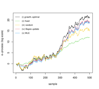
Figure 1: A few ways of constructing e-processes from likelihood ratio. Left: one run; Right: the average of 1000 runs (with average taken on the log values).

From this example, one can see that sequential e-variables could be more powerful (at least in this simple setting) whereas independent e-variables are more restrictive, but they allow for more merging methods, as we will see later.

Merging p-values and e-values

It may be interesting to note that the situations with merging p-values and e-values appear to be opposite. Merging independent p-values is in some sense trivial: for any measurable increasing function $F:[0,1]^{K}\to\mathbb{R}$ (intuitively, a test statistic), the function

$$G(p_{1},\dots,p_{K}):=\lambda(\{(q_{1},\dots,q_{K})\in[0,1]^{K}\mid F(q_{1},\dots,q_{K})\geq F(p_{1},\dots,p_{K})\}),$$

where $\lambda$ is the Lebesgue measure on $[0,1]^{K}$, is an ip-merging function, and any ip-merging function can be obtained in this way. On the other hand, merging arbitrarily dependent p-values is difficult, in the sense that the structure of the class of all p-merging functions is very complicated (see, e.g., [11], including a review of previous results). In the case of e-values, merging arbitrarily dependent e-values is trivial, at least in the case of symmetric merging functions: according to [12, Proposition 3.1], arithmetic mean essentially dominates any symmetric e-merging function (and [12, Theorem 3.2] gives a full description of the class of all symmetric e-merging functions). Merging independent e-values is difficult and is the topic of this paper.

Notation

We fix some notation throughout the paper. If $A$ is a measurable space, we let $A^{<K}$ stand for the measurable space $\bigcup_{k=0}^{K-1}A^{k}$, where $A^{0}=\{\Box\}$, with $\Box$ denoting the empty sequence. For $\mathbf{e}=(e_{1},\dots,e_{K})\in[0,\infty)^{K}$ and $k\in[K]$, we use $\mathbf{e}_{(k)}=(e_{1},\dots,e_{k})$ to represent the vector of the first $k$ components of $\mathbf{e}$, where $\mathbf{e}_{(0)}=\Box$ if $k=0$, and similarly for other vectors. Let $\mathcal{E}$ be the class of e-variables, i.e., nonnegative random variables $E$ on the underlying probability space satisfying $\mathbb{E}[E]\leq 1$.

3 Merging sequential e-values

We first define the notion of a gambling system and a test martingale. They form the basis of se-merging functions.

A gambling system is a measurable function $s:[0,\infty)^{<K}\to[0,1]$. The test martingale associated with the gambling system $s$ and initial capital $c\in[0,1]$ is the sequence of measurable functions $S_{k}:[0,\infty)^{K}\to[0,\infty)$, $k=0,\dots,K$, which is defined recursively by $S_{0}:=c$ and

$$S_{k+1}(\mathbf{e}):=S_{k}(\mathbf{e})\bigl{(}s(\mathbf{e}_{(k)})e_{k+1}+1-s(\mathbf{e}_{(k)})\bigr{)},\quad k=0,\dots,K-1.$$ (1)

(This is a martingale in the generalized sense of [8], which is slightly different from the same term in probability theory.) The intuition is that we observe $e_{1},\dots,e_{K}$ sequentially, start with capital at most 1, and at the end of step $k$ invest a fraction $s(\mathbf{e}_{(k)})$ of our current capital in $e_{k+1}$, leaving the remaining capital aside. We will also say that we gamble the fraction $s$ of our capital and refer to $s$ as our bet. Then $S_{k}(\mathbf{e})$, which depends on $\mathbf{e}$ only via $\mathbf{e}_{(k)}$, is our resulting capital at time $k$.

Lemma 1.

A convex combination of test martingales is a test martingale.

Proof.

The statement of the lemma follows from the following equivalent (and often useful) definition: a test martingale is a sequence of nonnegative functions $S_{k}:[0,\infty)^{K}\to[0,\infty)$, $k=0,\dots,K$, such that $S_{0}\leq 1$ and, for some measurable function $t:[0,\infty)^{<K}\to[0,\infty)$, we have

$$S_{k+1}(\mathbf{e})=S_{k}(\mathbf{e})+t(\mathbf{e}_{(k)})(e_{k+1}-1)$$ (2)

for all $k=0,\dots,K-1$ and all $\mathbf{e}\in[0,\infty)^{K}$. ∎

A martingale merging function is a function $F:[0,\infty)^{K}\to[0,\infty)$ that can be represented in the form $F=S_{K}$ for some test martingale $S_{k}$, $k=0,\dots,K$. An equivalent formulation is

$$S_{K}(\mathbf{e})=S_{0}\prod_{k=1}^{K}(1+s(\mathbf{e}_{(k-1)})(e_{k}-1)),$$ (3)

where $s$ is a gambling system. The following two results show that martingale merging functions are se-merging functions and any an se-merging function is dominated by a martingale merging function.

Lemma 2.

Any martingale merging function is an se-merging function.

Proof.

Let $E_{1},\dots,E_{K}$ be sequential e-variables in some probability space. It suffices to consider the case where $\mathbb{E}[E_{k}]=1$ for each $k=1,\dots,K$. Then $(S_{k}(E_{1},\dots,E_{K}),\mathcal{F}_{k})$, $k=0,\dots,K$, where $S_{k}$ is defined by (1) and $\mathcal{F}_{k}$ is the $\sigma$-algebra generated by $E_{1},\dots,E_{k}$, is a martingale. This immediately implies $\mathbb{E}[S_{K}(E_{1},\dots,E_{K})]\leq 1$. ∎

Theorem 1.

Any se-merging function is dominated by a martingale merging function.

Proof.

Let $F$ be an se-merging function; our goal is to construct a dominating martingale merging function. First we consider e-variables taking values in the set $2^{-n}\mathbb{N}$, where $\mathbb{N}:=\{0,1,\dots\}$; let $\mathcal{E}_{n}$ be the set of such e-variables. Extend $F$ to shorter sequences of e-values by

$$F_{n,K}(e_{1},\dots,e_{K}) :=F(e_{1},\dots,e_{K}),$$

$$F_{n,k}(e_{1},\dots,e_{k}) :=\sup_{E\in\mathcal{E}_{n}}\mathbb{E}[F_{n,k+1}(e_{1},\dots,e_{k},E)]$$ (4)

for all $e_{1},\dots,e_{K}\in 2^{-n}\mathbb{N}$ and $k=K-1,\dots,0$. It is clear that $F_{0}\leq 1$. By the duality theorem of linear programming, for any $k\in\{0,\dots,K-1\}$ and any $e_{1},\dots,e_{K}\in 2^{-n}\mathbb{N}$, there exists $s\in[0,1]$ such that

$$\forall e\in 2^{-n}\mathbb{N}:F_{n,k+1}(e_{1},\dots,e_{k},e)\leq F_{n,k}(e_{1},\dots,e_{k})(se+1-s).$$ (5)

Let us check carefully the application of the duality theorem. Let $c_{1},\dots,c_{N}$ be the first $N$ elements of the set $2^{-n}\mathbb{N}$ (namely, $c_{i}:=(i-1)2^{-n}$, $i=0,\dots,N-1$); we are interested in the case $N\to\infty$. Restricting $E$ in (4) to take values $c_{1},\dots,c_{N}$ with any probabilities $p_{1},\dots,p_{N}$, instead of $F_{n,k}(e_{1},\dots,e_{k})$ we will obtain the solution $F_{n,k,N}$ to the linear programming problem

$$c_{1}p_{1}+\dots+c_{N}p_{N} \leq 1$$ (6)

$$p_{1}+\dots+p_{N} =1$$ (7)

$$f_{1}p_{1}+\dots+f_{N}p_{N} \to\max,$$ (8)

where $p_{i}$ are nonnegative variables and $f_{i}:=F_{n,k+1}(e_{1},\dots,e_{k},c_{i})$, $i=1,\dots,N$. It is clear that the sequence $F_{n,k,N}$ is increasing in $N$ and tends to $F_{n,k}(e_{1},\dots,e_{k})$ as $N\to\infty$. The dual problem to (6)–(8) is $y_{1}+y_{2}\to\min$ subject to $y_{1}\geq 0$ and $c_{i}y_{1}+y_{2}\geq f_{i}$ for all $i\in\{1,\dots,N\}$. Then we will have the analogue

$$\forall e\in 2^{-n}\{0,\dots,N-1\}:F_{n,k+1}(e_{1},\dots,e_{k},e)\leq F_{n,k,N}(se+1-s)$$ (9)

of (5) when $y_{1}+y_{2}=F_{n,k,N}$ (which is the case for the optimal $(y_{1},y_{2})$) and $y_{1}=sF_{n,k,N}$. It is clear from (9) that $s\leq 1$, as $e=0$ is allowed. Let $s_{N}$ be an $s$ satisfying (9). Then any limit point of the sequence $s_{N}$ will satisfy (5).

We have proved the statement of the theorem for e-values in $2^{-n}\mathbb{N}$; now we drop this assumption. Let $(e_{1},\dots,e_{K})\in[0,\infty)^{K}$. For each $n$, let $e_{n,k}$ be the largest number in $2^{-n}\mathbb{N}$ that does not exceed $e_{k}$. Set

$$F_{k}(e_{1},\dots,e_{k}):=\lim_{n\to\infty}F_{n,k}(e_{n,1},\dots,e_{n,k}),$$

Then $F_{k}$ is a test martingale, and the fraction $s$ to gamble after observing $e_{1},\dots,e_{k}$ can be chosen as the smallest $s\in[0,1]$ satisfying

$$\forall e\in[0,\infty):F_{k+1}(e_{1},\dots,e_{k},e)\leq F_{k}(e_{1},\dots,e_{k})(se+1-s).$$ (10)

The set of such $s$ is obviously closed; let us check that it is non-empty. Let $s=s_{n}$ be a number in $[0,1]$ satisfying (5) with $e_{n,1},\dots,e_{n,k}$ in place of $e_{1},\dots,e_{k}$, respectively. Then any limit point of $s_{n}$ will satisfy (10). ∎

As we mentioned in Section 2, a martingale merging function is not necessarily increasing in all components. This is because $s(\mathbf{e}_{k-1})(e_{k}-1)$ in (3) is generally not increasing or decreasing in $\mathbf{e}_{(k)}$. Although monotonicity does not hold, any martingale merging function $F$ satisfies a notion of sequential monotonicity: for fixed $k\in[K]$ and $(e_{1},\dots,e_{k-1})\in[0,\infty)^{k-1}$, the function $e_{k}\mapsto F(e_{1},\dots,e_{k-1},e_{k},1,\dots,1)$ is increasing.

Example 1.

The non-monotonicity of $S_{K}$ appears naturally in an “exceed-and-stop” betting strategy: for some fixed $\alpha\in(0,1)$ and for each $k\in[K]$, if $S_{k}(\mathbf{e})\geq 1/\alpha$, then we choose $s(\mathbf{e}_{(k)})=0$ (which implies $s(\mathbf{e}_{(j)})=0$ for all $j\geq k$); otherwise we choose $s(\mathbf{e}_{(k)})>0$. Statistically, this corresponds a simple e-test strategy for a given type-I error $\alpha$. It is clear from (3) that $S_{K}$ is not increasing since $s(\mathbf{e}_{(k-1)})(e_{k}-1)$ is unbounded from above if $s(\mathbf{e}_{(k-1)})>0.$

Examples of martingale merging functions

The simplest non-trivial gambling system is $s:=1$; the corresponding test martingale with initial capital 1 is the product

$$S_{k}(e_{1},\dots,e_{K})=e_{1}\dots e_{k},$$

and the corresponding martingale merging function is the product

$$F(e_{1},\dots,e_{K}):=e_{1}\dots e_{K}.$$

This is the most standard se-merging function.

Another martingale merging function is the arithmetic mean

$$F(e_{1},\dots,e_{K}):=\frac{e_{1}+\dots+e_{K}}{K}.$$

This is in fact an e-merging function (the most important symmetric one, as explained in [12]). The corresponding test martingale is the mean

$$S_{k}(e_{1},\dots,e_{K}):=\frac{e_{1}+\dots+e_{k}+K-k}{K}.$$

(This is easiest to see using the equivalent definition (2).)

A more general class of martingale merging functions, introduced in [12], includes the U-statistics

$$U_{n}(e_{1},\dots,e_{K}):=\frac{1}{\binom{K}{n}}\sum_{\{k_{1},\dots,k_{n}\}\subseteq\{1,\dots,K\}}e_{k_{1}}\dots e_{k_{n}},\quad n\in\{0,1,\dots,K\}.$$ (11)

This is a martingale merging function because each addend in (11) is, and a convex combination of test martingales is a test martingale (Lemma 1).

Our final martingale merging function has an increasing sequence of numbers $1\leq K_{1}<\dots<K_{m}<K$ as its parameter and is defined as

$$F(e_{1},\dots,e_{K}):=\prod_{i=0}^{m}\frac{e_{K_{i}+1}+\dots+e_{K_{i+1}}}{K_{i+1}-K_{i}},$$

where $K_{0}$ is understood to be $0$ and $K_{m+1}$ is understood to be $K$. The corresponding test martingale is

$$S_{k}(e_{1},\dots,e_{K}):=\frac{\sum_{j=1}^{K_{1}}e_{j}}{K_{1}}\times\dots\times\frac{\sum_{j=K_{i-1}+1}^{K_{i}}e_{j}}{K_{i}-K_{i-1}}\times\frac{\sum_{j=K_{i}+1}^{k}e_{j}+K_{i+1}-k}{K_{i+1}-K_{i}},$$

where $i$ is the largest number such that $K_{i}\leq k$.

4 Anytime validity

In this section, we say that an e-variable $E$ is precise if $\mathbb{E}[E]=1$, and an se-merging function $F$ is precise if $\mathbb{E}[F(\mathbf{E})]=1$ for any vector $\mathbf{E}$ of precise and sequential e-values. This property is satisfied by all examples of merging functions in [12]. All supermartingales, martingales and stopping times are defined with respect to the filtration generated by $\mathbf{E}=(E_{1},\dots,E_{K})$.

In scientific discovery, experiments are often conducted sequentially in time, and a discovery may be reported at the time when enough evidence is gathered. Therefore, with a vector $\mathbf{E}$ of sequential e-values, it is desirable to require validity of a test at not only the fixed time $K$, but also a stopping time $\tau$. Such an approach produces an anytime-valid test. Fortunately, anytime validity is automatically achieved by using a test supermartingale: since $(S_{k}(\mathbf{E}))_{k=1,\dots,K}$ is a supermartingale, $S_{\tau}(\mathbf{E})$ is an e-variable for any stopping time $\tau$.

Conversely, if a sequence of functions $F_{k}:[0,\infty)^{K}\to[0,\infty)$, $k=0,1,\dots,K$, satisfies

1. anytime validity: $F_{\tau}(\mathbf{E})$ is an e-variable for any vector $\mathbf{E}$ of sequential e-values and any stopping time $\tau$;

2. precision: $F_{k}$ is precise for each $k\in[K]$,

then we can show that it is a test martingale.

Theorem 2.

For a sequence of functions $F=(F_{k})_{k=1,\dots,K}$, the following are equivalent:

1. $F$ is a test martingale (with $c=1$);

2. $F(\mathbf{E})$ is a martingale for any vector $\mathbf{E}$ of precise and sequential e-values;

3. $F$ is anytime valid and precise; i.e., it satisfies (a) and (b).

Proof.

The implications (i)$\Rightarrow$(ii) and (ii)$\Rightarrow$(iii) are straightforward. Below we show (iii)$\Rightarrow$(i).

Take any precise and sequential e-values $E_{1},\dots,E_{K}$, and let $\mathcal{F}=(\mathcal{F}_{k})_{k=1,\dots,K}$ be the natural filtration of $\mathbf{E}=(E_{1},\dots,E_{K})$.

Let $\tau$ be any ($\mathcal{F}$-)stopping time. First, we claim that $\mathbb{E}[F_{\tau}(\mathbf{E})]=1$ holds. To show this claim, for $j=1,\dots,K-1$ define $\tau_{j}=j$ if $\tau>j$ and $\tau_{j}=j+1$ if $\tau\leq j$. Clearly, $\tau_{j}$ is a stopping time for each $j$. Moreover, the realization of $(\tau,\tau_{1},\dots,\tau_{K-1})$ is always a permutation of $(1,\dots,K)$. Hence, using (b), we have

$$\mathbb{E}\left[F_{\tau}(\mathbf{E})+\sum_{j=1}^{K-1}F_{\tau_{j}}(\mathbf{E})\right]=\mathbb{E}\left[\sum_{k=1}^{K}F_{k}(\mathbf{E})\right]=K.$$

Using (a), $\mathbb{E}[F_{\tau_{j}}(\mathbf{E})]\leq 1$ for each $j$. This implies $\mathbb{E}[F_{\tau}(\mathbf{E})]\geq 1$. Therefore, $\mathbb{E}[F_{\tau}(\mathbf{E})]=1$ for any stopping time $\tau$.

If for some $k=1,\dots,K-1$, the event $A:=\{\mathbb{E}[F_{k+1}(\mathbf{E})\mid\mathcal{F}_{k}]>F_{k}(\mathbf{E})\}$ has a positive probability, then the stopping times $\eta:=k\mathds{1}_{A}+K\mathds{1}_{A^{c}}$ and $\eta^{\prime}:=(k+1)\mathds{1}_{A}+K\mathds{1}_{A^{c}}$ satisfy $\mathbb{E}[F_{\eta}(\mathbf{E})]<\mathbb{E}[F_{\eta^{\prime}}(\mathbf{E})]$, violating the property that $\mathbb{E}[F_{\tau}(\mathbf{E})]=1$ for any stopping time $\tau$. Hence, $\mathbb{P}(A)=0$. Similarly, $\mathbb{P}(\mathbb{E}[F_{k+1}(\mathbf{E})\mid\mathcal{F}_{k}]<F_{k}(\mathbf{E}))=0$. Therefore, $\mathbb{E}[F_{k+1}(\mathbf{E})\mid\mathcal{F}_{k}]=F_{k}(\mathbf{E})$ almost surely, and $(F_{k}(\mathbf{E}))_{k=1,\dots,K}$ is an $\mathcal{F}$-martingale.

Note that $F_{K}$ is an se-merging function. By Theorem 1, we have $F_{K}(\mathbf{E})\leq S_{K}(\mathbf{E})$ for some test martingale $(S_{k})_{k=1,\dots,K}$. Since $\mathbb{E}[F_{K}(\mathbf{E})]=\mathbb{E}[S_{K}(\mathbf{E})]$, we have $F_{K}(\mathbf{E})=S_{K}(\mathbf{E})$ almost surely. Using the fact that both $(F_{k}(\mathbf{E}))_{k=1,\dots,K}$ and $(S_{k}(\mathbf{E}))_{k=1,\dots,K}$ are martingales, we have, for $k=1,\dots,K$, almost surely

$$F_{k}(\mathbf{E})=\mathbb{E}[F_{K}(\mathbf{E})|\mathcal{F}_{k}]=\mathbb{E}[S_{K}(\mathbf{E})|\mathcal{F}_{k}]=S_{k}(\mathbf{E}).$$

Since $\mathbf{E}$ is arbitrary, we have $F_{K}=S_{K}$. ∎

Theorem 2 implies that, in order to get an anytime-valid and precise method for merging sequential e-values, the only tool one could rely on is the class of test martingales.

5 Merging independent e-values

In this section, we will study the more delicate situation of merging independent e-values. Since independent e-variables are sequential e-variables, the martingale merging methods in Section 3 are valid in this situation. The more interesting question is how many more merging functions are allowed for independent e-values.

We first explain the intuition, and then introduce the formal mathematical description. An important observation is that, in case e-values are independent, one may process them in any arbitrary order, instead of the fixed order for sequential e-values. Let us imagine that $K$ e-values are written on cards, which initially are lying face down so that their values are not shown. The decision maker needs to reveal these cards one by one, and bet on each card right before revealing it. In the case of sequential e-values, the order of revealing these cards is fixed (from card $1$ to card $K$), and the amount of bet on card $k+1$ (which has value $e_{k+1}$) is $s(\mathbf{e}_{(k)})$ in (1).

In case the e-values are independent, the decision maker can decide the order of revealing these e-values. Moreover, she can take an adaptive strategy for turning over the cards, that is, at each step, revealing a card based on what she sees on the previous cards (this view of picking random numbers is explained in in Kolmogorov [2, Section 2]). As in the case of constructing martingale merging functions, the decision maker also needs to decide the amount of bet at each step. Therefore, the strategy involves two decision variables, which e-value to reveal next, denoted by $\pi_{k+1}$, and how much to bet on this e-value, denoted by $s(\mathbf{e}^{\pi}_{(k)})$, where $\mathbf{e}^{\pi}_{(k)}=(e_{\pi_{1}},\dots,e_{\pi_{k}})$, and again $\mathbf{e}^{\pi}_{(0)}=\Box$. Although not explicitly reflected in the notation, one should keep in mind that $\pi_{k+1}$ is a function of $\mathbf{e}^{\pi}_{(k)}$. We write $\mathbf{e}^{\pi}=(e_{\pi_{1}},\dots,e_{\pi_{K}})$, which is the vector of e-values reordered by $\pi$.

Certainly, an average of the above procedures with different orders or different strategies is still an ie-merging function. This corresponds to a randomized betting strategy of the decision maker: at each step, she can generate $\pi(k+1)$ and $s(\mathbf{e}^{\pi}_{(k)})$ using some distributions that depend on the past observations and decisions.

We will make this procedure rigorous below. The order of revealing the e-values is modelled by $\pi=(\pi_{k})_{k\in[K]}$ where $\pi_{k}:[0,\infty)^{k-1}\to[K]$, and for any $\mathbf{e}\in[0,\infty)^{K}$, $\pi_{k}(\mathbf{e}^{\pi}_{(k-1)})\neq\pi_{j}(\mathbf{e}^{\pi}_{(j-1)})$ for distinct $j,k\in[K]$, meaning that you can only read the same e-value once. Equivalently, $\{\pi_{k}(\mathbf{e}_{(k-1)}^{\pi}):k\in[K]\}=[K].$ Such $\pi$ is called a reading strategy.

For a given gaming system $s:[0,\infty)^{<K}\to[0,1]$, a reading strategy $\pi:[0,\infty)^{<K}\to[K]$ and $c\in[0,1]$, a reordered test martingale is the sequence of measurable functions $S_{k}:[0,\infty)^{K}\to[0,\infty)$, $k=0,\dots,K$, given by $S_{0}^{s,\pi}:=c$ and

$$S^{s,\pi}_{k+1}(\mathbf{e}):=S^{s,\pi}_{k}(\mathbf{e})\left(s(\mathbf{e}^{\pi}_{(k)})e_{\pi_{k+1}}+1-s(\mathbf{e}^{\pi}_{(k)})\right),\quad k=0,\dots,K-1.$$ (12)

where we omit the argument in $\pi_{k+1}=\pi_{k+1}(\mathbf{e}^{\pi}_{(k)})$. An equivalent way to write (12) is

$$S_{k}^{s,\pi}(\mathbf{e})=S_{k}(\mathbf{e}^{\pi}),~{}~{}~{}k=0,1,\dots,K,$$

where $(S_{k})_{k=0,1,\dots,K}$ is the test martingale in (1) associated with $s$.

A generalized martingale merging function $F$ is a mixture (average) of $S_{K}^{s,\pi}$ above, that is,

$$F(\mathbf{e})=\mathbb{E}^{\mu}[S^{s,\pi}_{K}(\mathbf{e})]=\int S^{s,\pi}_{K}(\mathbf{e})\mathrm{d}\mu(s,\pi)\mbox{~{}~{}~{}~{}for $\mathbf{e}\in[0,\infty)^{K}$},$$ (13)

for some probability measure $\mu$ on the pair $(s,\pi)$. Note that $s$ and $\pi$ are not necessarily independent in general.

The generalized martingale merging functions form a subclass of the ie-merging functions, as the following proposition shows.

Proposition 2.

Any generalized martingale merging function is an ie-merging function.

Proposition 2 essentially follows from the following lemma. For this proposition, we only need the first statement of the lemma.

Lemma 3.

Let $E_{1},\dots,E_{K}$ be independent e-variables, and $\pi$ a reading strategy. Recursively define $E^{\pi}_{k}=E_{\pi_{k}(E_{1}^{\pi},\dots,E_{k-1}^{\pi})}$ for $k\in[K]$. Then $E_{1}^{\pi},\dots,E_{K}^{\pi}$ are sequential e-variables. If $E_{1},\dots,E_{K}$ are iid, then so are $E_{1}^{\pi},\dots,E_{K}^{\pi}$.

Proof.

Denote by $\mathbf{E}^{\pi}_{(k)}=(E_{1}^{\pi},\dots,E_{k}^{\pi})$ for $k\in\{0,1,\dots,K\}$ and by $A^{\pi}_{k}=[K]\setminus\{\pi_{1}(\mathbf{E}^{\pi}_{(0)}),\pi_{2}(\mathbf{E}^{\pi}_{(1)}),\dots,\pi_{k}(\mathbf{E}^{\pi}_{(k-1)})\}$ for $k\in[K]$, which is the set of possible values $\pi_{k+1}(\mathbf{E}^{\pi}_{(k)})$ can take. Note that for $j\in A^{\pi}_{k}$, $E_{j}$ is independent of $\mathbf{E}^{\pi}_{(k)}$. For any measurable function $f:\mathbb{R}\to\mathbb{R}$ and $k=1,\dots,K-1$, we have

$$\mathbb{E}\left[f(E^{\pi}_{k+1})\mid E_{1}^{\pi},\dots,E_{k}^{\pi}\right] =\sum_{j\in[K]}\mathbb{E}\left[f(E_{j})\mathds{1}_{\{j=\pi_{k+1}(\mathbf{E}^{\pi}_{(k)})\}}\mid\mathbf{E}^{\pi}_{(k)}\right]$$

$$=\sum_{j\in A^{\pi}_{k}}\mathds{1}_{\{j=\pi_{k+1}(\mathbf{E}^{\pi}_{(k)})\}}\mathbb{E}\left[f(E_{j})\right].$$ (14)

Taking $f$ as the identity in (14), we get $\mathbb{E}\left[f(E_{j})\right]\leq 1$ for $j\in A_{k}$, and hence $\mathbb{E}\left[f(E^{\pi}_{k+1})\mid E_{1}^{\pi},\dots,E_{k}^{\pi}\right]\leq 1$. This shows that $E_{1}^{\pi},\dots,E_{K}^{\pi}$ are sequential e-variables.

If $E_{1},\dots,E_{K}$ are iid, then (14) yields $\mathbb{E}[f(E^{\pi}_{k+1})\mid E_{1}^{\pi},\dots,E_{k}^{\pi}]=\mathbb{E}[f(E_{1})]$ and $\mathbb{E}[f(E^{\pi}_{k+1})]=\mathbb{E}[f(E_{1})]$ for any measurable $f$. This shows that $E_{k+1}^{\pi}$ is independent of $E_{1}^{\pi},\dots,E_{k}^{\pi}$ and identically distributed as $E_{1}$. Hence, $E_{1}^{\pi},\dots,E_{K}^{\pi}$ are iid. ∎

In the first statement of Lemma 3, $E^{\pi}_{1},\dots,E^{\pi}_{K}$ are sequential e-variables but not necessarily independent. For instance, consider a setting where $E_{1}$ and $E_{2}$ are uniform on $[0,2]$ and $E_{3}=1$. The strategy $\pi$ is specified by $\pi_{1}=1$, $\pi_{2}(e)=2\mathds{1}_{\{e<1\}}+3\mathds{1}_{\{e\geq 1\}}$. It is clear that $E^{\pi}_{1}$ and $E^{\pi}_{2}$ are not independent.

Proof of Proposition 2.

Let $\mathbf{E}=(E_{1},\dots,E_{K})$ be a vector of independent e-variables. It suffices to consider $S^{s,\pi}_{K}(\mathbf{E})$ in (12) for a deterministic pair $(s,\pi)$, because a generalized martingale merging function is a mixture of $S_{K}^{s,\pi}$, and taking a mixture of e-variables yields an e-variable. Note that $S_{K}^{s,\pi}(\mathbf{E})=S_{K}(\mathbf{E}^{\pi})$, where $\mathbf{E}^{\pi}=(E_{1}^{\pi},\dots,E_{K}^{\pi})$ in Lemma 3. Hence, $\mathbb{E}[S^{s,\pi}_{K}(\mathbf{E})]\leq 1$ follows from Lemmas 2 and 3. ∎

The following is an example of a generalized martingale merging function that is not an se-merging function.

Example 2.

The following function is taken from [12, Remark 4.3], where it is shown that

$$F(e_{1},e_{2}):=\frac{1}{2}\left(\frac{e_{1}}{1+e_{1}}+\frac{e_{2}}{1+e_{2}}\right)\left(1+e_{1}e_{2}\right)$$ (15)

is an ie-merging function. We will check that $F$ is also a generalized martingale merging function, notice that the symmetric expression (15) can be represented as the arithmetic average of

$$\frac{e_{1}}{1+e_{1}}\left(1+e_{1}e_{2}\right)=e_{1}\left(\frac{1}{1+e_{1}}+\frac{e_{1}}{1+e_{1}}e_{2}\right)$$

and the analogous expression with $e_{1}$ and $e_{2}$ interchanged. The generalized gambling strategy producing (15) starts from uncovering $e_{1}$ or $e_{2}$ with equal probabilities and investing all the capital in the chosen e-variable. If $e_{1}$ is uncovered first, it then invests a fraction of $e_{1}/(1+e_{1})$ of its current capital into $e_{2}$. And if $e_{2}$ is uncovered first, it invests a fraction of $e_{2}/(1+e_{2})$ of its current capital into $e_{1}$.

Let us now check that $F$ is not an se-merging function. By the symmetry of $F$, we can assume, without loss of generality, that we first observe the e-variable $E_{1}$ producing $e_{1}$ and then observe $E_{2}$ producing $e_{2}$. Had $F$ been an se-merging function,

$$G(e_{1}):=\sup_{E_{2}\in\mathcal{E}}\mathbb{E}[F(e_{1},E_{2})]$$

would have produced an e-variable when plugging in $e_{1}=E_{1}$. However, using the convexity of the functions $x/(1+x)$, $x$, and $x^{2}/(1+x)$ of $x\in[0,\infty)$, we obtain

$$G(e_{1})=\sup_{E_{2}\in\mathcal{E}}\mathbb{E}[F(e_{1},E_{2})]=\max\left(e_{1},\frac{e_{1}+1}{2}\right),$$

where the maximum is attained at some $E_{2}$ that takes two values, one of which is 0. Note that if $\mathbb{E}[E_{1}]=1$, then $\mathbb{E}[G(E_{1})]>1$ unless $E_{1}=1$ with probability $1$. Hence, $F$ is not an se-merging function.

Example 3.

In case $K=2$, $\pi$ is specified by $\pi(1)$ which does not depend on any observed e-values. Hence, the bet $s$ can be chosen separately on the events $\{\pi(1)=1\}$ and $\{\pi(1)=2\}$, and no randomization is needed as shown by Lemma 1. Therefore, we can write all generalized martingale merging functions in (13) as

$$(e_{1},e_{2})\mapsto\beta(1+a_{1}\tilde{e}_{1})(1+g_{1}(e_{1})\tilde{e}_{2})+(1-\beta)(1+a_{2}\tilde{e}_{2})(1+g_{2}(e_{2})\tilde{e}_{1}),$$ (16)

where $\tilde{e}_{1}=e_{1}-1$, $\tilde{e}_{2}=e_{2}-1$, $\beta,a_{1},a_{2}\in[0,1]$, and $h_{1},h_{2}:[0,\infty)\to[0,1]$. To interpret (16) as a randomized reordered test martingale, $\beta$ is the probability of $\pi(1)=1$, $a_{1},a_{2}$ are the first-round bets, and $g_{1},g_{2}$ are the second-round bets.

In view of Theorem 1, one may wonder whether any ie-merging function is dominated by a generalized martingale merging function. The answer is no, as the following counter-example shows.

Example 4.

Fix a constant $c>1$ and define the function $G:[0,\infty)^{2}\to\mathbb{R}$ by

$$G(\mathbf{e})=\mathds{1}_{[0,c)^{2}}(\mathbf{e})+(2c-1)\mathds{1}_{[c,\infty)^{2}}(\mathbf{e}).$$

Take any two independent e-variables $E_{1},E_{2}$, and write $a=\mathbb{P}(E_{1}\geq c)$ and $b=\mathbb{P}(E_{2}\geq c)$. Markov’s inequality gives $a,b\leq 1/c$, which implies $1/a+1/b\geq 2c$, and thus $a+b\geq 2c(ab)$. We can verify

$$\mathbb{E}[G(E_{1},E_{2})] =\mathbb{P}(E_{1}<c)\mathbb{P}(E_{2}<c)+(2c-1)\mathbb{P}(E_{1}\geq c)\mathbb{P}(E_{2}\geq c)$$

$$=1-a-b+2c(ab)\leq 1.$$

Hence, $G$ is an ie-merging function. We can show that $G$ is not dominated by any generalized martingale merging function $F$. Suppose otherwise. We can assume that $F$ has the form (16). Since $F\geq G$, we know that $F=1$ on $[0,1]^{2}$, which implies that $a_{1}=a_{2}=0$. This gives $F(e_{1},e_{2})\leq\beta e_{1}+(1-\beta)e_{2}$. However, $G(c,c)=2c-1$ whereas $F(c,c)\leq c<2c-1$, a contradiction.

6 Conclusion

Regarding the merging functions of independent or sequential e-values, there are a few open questions.

1. It is unclear in which a practical setting constructing independent e-values performs better than constructing sequential but dependent e-values. Since independent e-values are more restrictive to construct (cf. the example of likelihood ratios in Section 2), it would only be valuable to construct them if they carry more statistical power in some situations.

2. It would be interesting to find simple, and perhaps practically useful, ie-merging functions that are not dominated by a generalized martingale merging function.

3. It remains unclear whether any increasing ie-merging function is dominated by a generalized martingale merging function; note that the function $G$ in Example 4 is not increasing.

4. We may further require an ie-merging function to be precise; that is, for independent e-variables with mean $1$, the function produces an e-variable with mean $1$. Is every ie-merging function with this requirement necessarily a generalized martingale merging function?

References

• Grünwald et al. [2020] Peter Grünwald, Rianne de Heide, and Wouter M. Koolen. Safe testing. Technical Report arXiv:1906.07801 [math.ST], arXiv.org e-Print archive, June 2020.
• Kolmogorov [1963] Andrei N. Kolmogorov. On tables of random numbers. Sankhyā. Indian Journal of Statistics A, 25:369–376, 1963.
• Loveland [1966a] Donald Loveland. The Kleene hierarchy classification of recursively random sequences. Transactions of the American Mathematical Society, 125:497–510, 1966a.
• Loveland [1966b] Donald Loveland. A new interpretation of the von Mises concept of random sequence. Zeitschrift für Mathematische Logik und Grundlagen der Mathematik, 12:279–294, 1966b.
• Mises [1928] Richard von Mises. Wahrscheinlichkeit, Statistik, und Wahrheit. Springer, Berlin, 1928. English translation: Probability, Statistics and Truth. William Hodge, London, 1939.
• Ramdas et al. [2020] Aaditya Ramdas, Johannes Ruf, Martin Larsson, and Wouter Koolen. Admissible anytime-valid sequential inference must rely on nonnegative martingales. arXiv preprint arXiv:2009.03167, 2020.
• Shafer [2021] Glenn Shafer. Testing by betting: A strategy for statistical and scientific communication. Journal of the Royal Statistical Society: Series A (Statistics in Society), 184(2):407–431, 2021.
• Shafer and Vovk [2019] Glenn Shafer and Vladimir Vovk. Game-Theoretic Foundations for Probability and Finance. Wiley, Hoboken, NJ, 2019.
• Shafer et al. [2011] Glenn Shafer, Alexander Shen, Nikolai Vereshchagin, and Vladimir Vovk. Test martingales, Bayes factors, and p-values. Statistical Science, 26:84–101, 2011.
• Ville [1939] Jean Ville. Etude critique de la notion de collectif. Gauthier-Villars, Paris, 1939.
• Vovk and Wang [2020] Vladimir Vovk and Ruodu Wang. Combining p-values via averaging. Biometrika, 107(4):791–808, 2020.
• Vovk and Wang [2021] Vladimir Vovk and Ruodu Wang. E-values: Calibration, combination and applications. The Annals of Statistics, 49(3):1736–1754, 2021.
• Wang and Wang [2015] Bin Wang and Ruodu Wang. Extreme negative dependence and risk aggregation. Journal of Multivariate Analysis, 136:12–25, 2015.
• Wang and Ramdas [2021] Ruodu Wang and Aaditya Ramdas. False discovery rate control with e-values. Journal of the Royal Statistical Society Series B, 2021.
• Wang and Ramdas [2022] Ruodu Wang and Aaditya Ramdas. E-values as unnormalized weights in multiple testing. arXiv preprint arXiv:2204.12447, 2022.