Rule Covering for Interpretation and Boosting

Abstract

We propose two algorithms for interpretation and boosting of tree-based ensemble methods. Both algorithms make use of mathematical programming models that are constructed with a set of rules extracted from an ensemble of decision trees. The objective is to obtain the minimum total impurity with the least number of rules that cover all the samples. The first algorithm uses the collection of decision trees obtained from a trained random forest model. Our numerical results show that the proposed rule covering approach selects only a few rules that could be used for interpreting the random forest model. Moreover, the resulting set of rules closely matches the accuracy level of the random forest model. Inspired by the column generation algorithm in linear programming, our second algorithm uses a rule generation scheme for boosting decision trees. We use the dual optimal solutions of the linear programming models as sample weights to obtain only those rules that would improve the accuracy. With a computational study, we observe that our second algorithm performs competitively with the other well-known boosting methods. Our implementations also demonstrate that both algorithms can be trivially coupled with the existing random forest and decision tree packages.

1 Introduction

Although their prediction performances are remarkable, tree-based ensemble methods are difficult to interpret due to large number of trees in the trained model. Among these methods, Random Forest algorithm is probably the most frequently used alternative for solving classification and regression problems arising in different domains [2]. This performance versus interpretability trade-off leads to the following two main questions in our work: Given a trained random forest, can we obtain an interpretable representation with mathematical programming that shows a performance close-enough to the overall forest? Using a similar mathematical programming model, can we come up with a learning algorithm, which generates only those rules that improve the performance of a base tree?

To answer these questions, we focus on the rules constituting the trees in the forest and propose two algorithms based on mathematical programming models. The model in the first algorithm extracts the rules corresponding to the leaves of the forest that result in the minimum total impurity while covering all the samples. With this algorithm, we are able to mimick the performance of the original forest with a significantly few number of rules (most of the time even less than the number of rules in a regular decision tree). Being encouraged with these results, we then propose our second algorithm based on selective generation of rules. This algorithm improves the total impurity gradually by solving a series of linear programming problems. This approach is a variant of the column generation algorithm in mathematical optimization. In our scheme, we use the dual optimal solutions of the linear programs as the sample weights. We also observe that this scheme has close ties to well-known ideas in boosting methods [13, 14, 17]. Thus, rule extraction and boosting are the two keywords that help us to review the related literature.

Friedman and Popescu [9] propose RuleFit method to extract rules from ensembles. The authors use decision trees as base learners, where each node of the decision tree corresponds to a rule. They present an ensemble generation algorithm to obtain a rule set. Then, they solve a linear regression problem that minimizes the loss with a lasso penalty for selecting rules. Meinshausen [15] presents a similar approach, called Node Harvest, which relies on rules generated by a tree ensemble. Node Harvest minimizes the quadratic loss function by partitioning the samples and relaxing the integrality constraints on the weights. Even though the algorithm does not constrain the number of rules, the author observes that only a small number of rules are used. Mashayekhi and Gras [11] propose coverage of the samples in the training set by the rules generated by Random Forest algorithm. They create a score for each rule by considering the percentage of correctly and incorrectly classified samples as well as the rule length. By using a hill climbing algorithm, they are able to obtain slightly lower accuracy with much fewer rules than random forest. Extending this work, Mashayekhi and Gras [12] propose three different algorithms to extract if-then rules from decision tree ensembles. The authors then compare their algorithms with both RuleFit and Node Harvest. All these approaches use accuracy values to construct the objective functions. Interpretability in terms of reducing the number of rules is achieved by using lasso penalties. Our first algorithm, on the other hand, reduces the number of rules directly through the objective function.

Gradient boosting algorithms use a sequence of weak learners and build a model iteratively [7, 13, 8]. At each iteration the boosting algorithm focuses on the misclassified samples by adjusting their weights with respect to the errors of the previous iterations. A boosting method that uses linear programming is called LPBoost [5]. This algorithm uses weak learners to maximize the margins separating the different classes. Like us, the authors also use column generation to create the weak learners iteratively. The final ensemble then becomes a weighted combination of the weak learners. The approach can accept decision stumps or decision trees as weak learners. However, decision trees can perform badly in terms of convergence and solution accuracy, if the dual variables associated with margin classification are not constrained. Unlike LPBoost, we use the duals as sample weights in our column generation routine. Another boosting method based on mathematical programming is called IPBoost [16]. This approach uses binary decision variables corresponding to misclassification by a predetermined margin. Due to binary decision variables, the authors resort to an integer programming solution technique called branch-and-bound-and-price. Dash et al. [4] also use column generation to learn Boolean decision rules in either disjunctive normal form or conjunctive normal form. They solve a sequence of integer programming problems for pricing the columns. They choose to restrict the number of selected clauses as a user-defined hyperparameter for improving interpretability. Bertsimas and Dunn [1] propose an integer programming formulation to create optimal decision trees for multi-class classification. They present two approaches with respect to node splitting. The first approach is more general but less interpretable. The second more interpretable model considers the values of one feature for node splitting. One advantage of their model is that it does not rely on an assumption for the nature of the values of the features. Günlük et al. [10] propose a binary classification tree formulation for only categorical features. The idea can be extended to numerical variables by using thresholding. The approach is less general than the approach presented by Bertsimas and Dunn [1], but has some advantages like the number of integer variables being independent of the training dataset size. Firat et al. [6] propose a column generation based heuristic for learning decision tree. The approach is based on generating decision paths and can be used for solving instances with tens of thousands of observations.

In the light of this review, we make the following contributions to the literature: We propose a new mathematical programming approach for interpretation and boosting of random forests and decision trees, respectively. Unlike other work in the literature, the objective function in our models aims at minimizing both the total impurity and the number of selected rules. When applied to a trained random forest for interpretation, our first algorithm obtains significantly few number of rules with an accuracy level close to the random forest model. Our second algorithm is a new boosting method based on rule generation and linear programming. As a novel approach, the algorithm uses dual information to weigh samples in order to increase the coverage with less impure rules. In our computational study, we demonstrate that both algorithms are remarkably easy to implement within a widely-used machine learning package. Without any fine tuning, we obtain quite promising numerical results with both algorithms showing the potential of the rule covering for interpretation and boosting.

2 Minimum rule cover: interpretation of forests

Let $(\bm{x}_{i},y_{i})$, $i\in\mathcal{I}$ be the set of samples, where the vector $\bm{x}_{i}\in\mathcal{X}$ and the scalar $y_{i}\in\mathcal{K}$ denote the input sample and the output class, respectively. We shall assume in the subsequent part that the learning problem at hand is a classification problem. However, our discussion here can be extended to regression problems as well (we elaborate on this point in Section S.3.).

Suppose that a Random Forest algorithm is trained on this dataset and a collection of trees is grown. Given one of these trees, we can easily generate the path $j$ from the root node to a leaf node that results in a subset of samples $\bm{x}_{i}$, $i\in\mathcal{I}(j)\subseteq\mathcal{I}$. Actually, these paths constitute the rules that are later used for classification with majority voting. Each rule corresponds to a sequence of if-then clauses and it is likely that some of these sequences may appear multiple times. We denote all such rules in all trees by set $\mathcal{J}$. Clearly, the size of $\mathcal{J}$ is quite large. Therefore, we next construct a mathematical programming model that aims at selecting the minimum number of rules from the trained forest while preserving the performance. We also make sure that all samples are covered with the selected rules.

As rule $j\in\mathcal{J}$ corresponds to a leaf node, we can also evaluate the node impurity, $w_{j}$. Two most common measures for evaluating the node impurity are known as Gini and Entropy criteria. We further introduce the binary decision variables $z_{j}$ that mark whether the corresponding rules $j\in\mathcal{J}$ are selected or not. The cost of $w_{j}$ is incurred, when $z_{j}=1$. Note that if we use only these impurity evaluations as the objective function coefficients (costs), then the model would tend to select many rules that cover only a few samples, which are likely to be pure nodes. However, we want to advocate the use of fewer rules in the model so that the resulting set of rules is easy to interpret. In other words, we also aim at minimizing the number of rules along with the impurity cost. Therefore, we replace the cost coefficient so that selecting excessive number of rules is penalized. Our mathematical programming model then becomes:

$$\begin{array}[]{lll}\mbox{minimize\hskip 11.38109pt}&\sum_{j\in\mathcal{J}}(1+w_{j})z_{j}&\\[5.69054pt] \mbox{subject to\hskip 11.38109pt}&\sum_{j\in\mathcal{J}(i)}z_{j}\geq 1,&i\in\mathcal{I},\\[5.69054pt] &z_{j}\in\{0,1\},&j\in\mathcal{J},\end{array}$$ (1)

where $\mathcal{J}(i)$, $i\in\mathcal{I}$ is the set of rules prescribing all the leaves involving sample $\bm{x}_{i}$. In other words, sample $i$ is covered with the rules in subset $\mathcal{J}(i)\subseteq\mathcal{J}$.

The mathematical programming model (1) is a standard weighted set covering formulation, where sets and items correspond to rules and samples, respectively. Although set covering problem is NP-hard, current off-the-shelf solvers are capable of providing optimal solutions to moderately large instances. In case the integer programming formulation becomes difficult to solve, there are also powerful heuristics that return approximate solutions very quickly. One such approach is the well-known greedy algorithm proposed by Chvatál [3]. Algorithm 3 shows the steps of this heuristic using our notation. Recently, Chvatál’s greedy algorithm, as we implement here, has been shown to perform quite well on a set of test problems when compared against several more recent heuristics [18]. Thus, we have reported our results also with this algorithm in Section 4. Clearly, this particular heuristic can be replaced with any other approach solving the set covering problem. Since these heuristics provide an approximate solution, we denote the resulting set of rules by $\hat{\mathcal{J}}$, and by definition, the cardinality of set $\hat{\mathcal{J}}$ is larger than the cardinality of the optimal set of rules obtained by solving (1).

Algorithm 1 gives the steps of our minimum rule cover algorithm (MIRCO). The algorithm takes as input the trained random forest model and the training dataset. Note that after running Algorithm 1, we obtain a subset of rules $\hat{\mathcal{J}}$ that can also be used for classifying out-of-sample points (test set) with majority voting. If we denote the predicted class of test sample $\bm{x}_{0}$ with $C(\bm{x}_{0},\hat{\mathcal{J}})$, then

$$C(\bm{x}_{0},\hat{\mathcal{J}})=\arg\max_{k\in\mathcal{K}}\big{\{}\sum_{j\in\hat{\mathcal{J}}}n_{jk}\mathds{L}_{j}(\bm{x}_{0})\big{\}},$$ (2)

where $n_{jk}$ stands for the number of samples from class $k$ in leaf $j$, and $\mathds{L}_{j}(\bm{x}_{0})$ is an operator showing whether $\bm{x}_{0}$ satisfies the sequence of clauses corresponding to leaf $j$. In fact, testing in this manner would be a natural approach for evaluating the performance of MIRCO. Since our main objective is to interpret the underlying model obtained with Random Forest algorithm, we hope that this subset of rules would obtain a classification performance closer to the performance obtained with all the rules in set $\mathcal{J}$. We show with our computational study in Section 4 that this is indeed the case.

Input : Random forest model RF; training dataset $(\bm{x}_{i},y_{i})$, $i\in\mathcal{I}$

1 $\mathcal{J}=\emptyset$;

2 for Tree in RF do

3       $\mathcal{J}\leftarrow\mathcal{J}\cup\text{(rules in {Tree})}$;

4      

5 end for

6

7Evaluate impurities $w_{j}$, $j\in\mathcal{J}$ using $(\bm{x}_{i},y_{i})$, $i\in\mathcal{I}$;

8

9Construct sets $\mathcal{J}(i)$, $i\in\mathcal{I}$ ;

10

11Solve model (1) with Algorithm 3;

12

13Return $\hat{\mathcal{J}}$;

Algorithm 1 MIRCO

Figure 1 shows an example set of of rules obtained with MIRCO on a small data set. Clearly, the resulting set of rules does not correspond to a decision tree. On one hand, this implies that we cannot simply select one of the trees grown by the Random Forest algorithm and replace its leaves with the set of rules obtained with MIRCO. Consequently, multiple rules may cover the same test sample, in which case we can again use majority voting to determine its class. Region A in Figure 1 shows that any test sample in that region will be classified with two overlapping rules. On the other hand, there is also the risk that the entire feature space is not covered by the subset of rules. In Figure 1 such a region is marked as B, where none of the rules cover this region. Therefore, if one decides to use only the rules in $\hat{\mathcal{J}}$ as a classifier, then some of the samples in the test set may not be classified at all. This is an anticipated behaviour, since MIRCO guarantees to cover only those samples that are used to train the Random Forest algorithm. Our numerical results show that the percentages of test samples that MIRCO fails to classify are quite low.

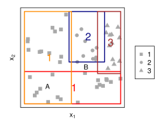
Figure 1: A toy example illustrating that MIRCO does not necessarily correspond to a tree. Rectangles denote the regions obtained with the rules in $\hat{\mathcal{J}}$. The numbers in the rectangles depict the classification results corresponding to three classes shown with three different markers.

Notice that the entire set of rules used by MIRCO does not have to be constructed after training a Random Forest algorithm. If there is an oracle that provides many rules to construct the set $\mathcal{J}$, then we can still (approximately) solve the mathematical programming model (1) and obtain the resulting set of rules. In fact, the development of this oracle decouples our discussion from training a forest. In the next section, we propose such an oracle that generates the necessary rules on the fly.

3 RCBoost: rule cover boosting

The main difficulty with the set covering problem is the integrality condition on the decision variables. When this condition is ignored, the resulting problem is a simple linear programming problem that can be solved quite efficiently. For the same reason, many approximation methods devised for the set covering problem are based on considering the linear programming relaxation of (1). Formally, the relaxed problem simply becomes:

$$\begin{array}[]{lllc}\mbox{minimize\hskip 11.38109pt}&\sum_{j\in\mathcal{J}}(1+w_{j})z_{j}&&\\[5.69054pt] \mbox{subject to\hskip 11.38109pt}&\sum_{j\in\mathcal{J}(i)}z_{j}\geq 1,&i\in\mathcal{I},\hskip 34.1433pt(\lambda_{i})\\[5.69054pt] &z_{j}\geq 0,&j\in\mathcal{J},&\end{array}$$ (3)

where $\lambda_{i}$, $i\in\mathcal{I}$ denote the dual variables corresponding to the constraints. After solving this problem, we obtain both the primal and the dual optimal solutions. As we will discuss shortly, the optimal dual variables bear important information about the sample points. Since we relax the integrality restrictions, one suggestion could be rewriting the objective as solely the minimization of total impurity. We refrain from such an approach because when there are many pure leaves, then the corresponding rule does not contribute to the objective function value ($w_{j}=0$) and the corresponding $z_{j}$ variable becomes free to attain any value. This implies that the primal problem has multiple optimal solutions, and hence causing degeneracy in the dual.

We have seen in the previous section that problem (3) may easily have quite many variables (columns). One standard approach to solve this type of linear programming problems is based on iterative generation of only necessary variables that would lead to an improvement in the objective function value. This approach is known as column generation. The main idea is to start with a set of columns (column pool) and form a linear programming problem, called the restricted master problem (RMP). After solving the restricted master problem, the dual optimal solution is obtained. Then using this dual solution, a pricing subproblem is solved to find the columns with negative reduced costs. These columns are the only candidates for improving the objective function value when they are added to the column pool. The next iteration continues with obtaining the optimal dual solution of the new restricted master problem with the extended column pool. Again, the pricing subproblem is solved to find the columns with negative reduced costs. If there is no such column, then the column generation algorithm terminates.

Suppose that we denote the column pool in the restricted master problem at iteration $t$ of column generation algorithm by $\mathcal{J}_{t}$. Then, we solve the following linear programming problem:

$$\begin{array}[]{lllc}\mbox{minimize\hskip 11.38109pt}&\sum_{j\in\mathcal{J}_{t}}(1+w_{j})z_{j}&&\\[5.69054pt] \mbox{subject to\hskip 11.38109pt}&\sum_{j\in\mathcal{J}_{t}(i)}z_{j}\geq 1,&i\in\mathcal{I},&\hskip 11.38109pt(\lambda^{t}_{i})\\[5.69054pt] &z_{j}\geq 0,&j\in\mathcal{J}_{t},&\end{array} (\mathcal{J}_{t})$$ (RMP)

where $\lambda^{t}_{i}$ denotes the dual variable corresponding to constraint $i\in\mathcal{I}$ at iteration $t$, and $\mathcal{J}_{t}(i)$ stands for the rules in $\mathcal{J}_{t}$ that cover sample $i$. The reduced cost of rule $j\in\mathcal{J}_{t}$ is simply given by

$$\bar{w}_{j}=(1+w_{j})-\sum_{i\in\mathcal{I}(j)}\lambda^{t}_{i}.$$ (4)

The necessary rules that would improve the objective function value in the next iteration are the ones with negative reduced costs. In all this discussion, the key point is, in fact, the pricing subproblem, which would generate the rules with negative reduced costs. Recall that the columns in this approach are constructed by the rules in our setting. Thus, in the remaining part of this section, we shall use the term “rule pool” instead of “column pool.”

Algorithm 2 shows the training process of the proposed rule cover boosting (RCBoost) algorithm. The steps of the algorithm is also given in Figure 2. Here, DecisionTree routine plays the role of the pricing subproblem. The parameter of this routine is a vector, which is used to assign different weights to the samples. To obtain rules with negative reduced costs, the dual optimal solution of the restricted master problems is passed as the sample weight vector (line 2). If there are rules with negative reduced costs (line 2), then these are added to the rule pool $\mathcal{J}^{*}$ in line 2. Otherwise, the algorithm terminates (line 2). Note that a bound on the maximum number of RMP calls can also be considered as a hyperparameter. The resulting set or rules in the final pool constitute the classifier (line 2). Like in Random Forest algorithm, a test point is classified using the majority voting system among all the rules (if-then clauses) that are satisfied. Note that there is no danger of failing to classify a test sample like MIRCO, since the initial rule pool is constructed with a decision tree (line 2). The output set of rules $\mathcal{J}^{*}$ is then used for classifying out-of-sample point with majority voting as in (2). That is, $C(\bm{x}_{0},\mathcal{J}^{*})$ is the predicted class for $\bm{x}_{0}$.

Input : Training data $(\bm{x}_{i},y_{i})$, $i\in\mathcal{I}$

1 $\bar{\bm{\lambda}}=(1,1,\dots,1)$;

2 $\mathcal{J}^{*}\leftarrow\text{{DecisionTree}}(\bar{\bm{\lambda}})$;

3 for $t=1,2,\dots$ do

4       $\bm{\lambda}^{t}\leftarrow\text{{RMP}}(\mathcal{J}^{*})$;

5       $\bar{\bm{\lambda}}\leftarrow\bar{\bm{\lambda}}+\bm{\lambda}^{t}$;

6       $\bar{\mathcal{J}}\leftarrow\text{{DecisionTree}}(\bar{\bm{\lambda}})$;

7       $\bar{\mathcal{J}}^{-}=\{j\in\bar{\mathcal{J}}~{}:~{}\bar{w_{j}}<0\}$;

8       if $\bar{\mathcal{J}}^{-}=\emptyset$ then

9             break;

10            

11       end if

12      $\mathcal{J}^{*}\leftarrow\mathcal{J}^{*}\cup\bar{\mathcal{J}}^{-}$;

13      

14 end for

15Return $\mathcal{J}^{*}$;

Algorithm 2 RCBoost

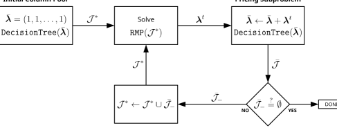
Figure 2: Flowchart of RCBoost

As line 2 shows, we accumulate the dual vectors at every iteration. This is because many of the dual variables quickly become zero as either the corresponding primal constraints are inactive or the dual optimal solution becomes degenerate. So, we make sure with the accumulation that all the sample weights remain nonzero. We should also note that calling the decision tree algorithm with (cumulative) sample weights is a proxy to the pricing subproblem. Because, the actual pricing subproblem is supposed to search for the rules with negative reduced costs. However, we argue that using such a proxy is still sensible. We appeal to the theory of sensitivity analysis in linear programming and the role of sample weights in boosting algorithms. An optimal dual variable shows the change in the optimal objective function, when the right-hand side of this constraint (all ones in our case) is slightly adjusted. Since each constraint corresponds to the samples in (1), the corresponding optimal dual variables show us the role of these samples for changing the objective function value. In fact the reduced cost calculation in (4) also bears the same intuition and promotes having a rule with low impurity and large dual variables. Thus, if the samples with large dual values (weights) belong to the same class, then they are more likely to be classified within the same leaf (rule) to decrease the impurity. On the other hand, if these samples belong to different classes, then putting them into separate leaves also yields a decrease in impurity. This is precisely what the sample weights try to achieve for boosting methods, where the weights for the incorrectly classified samples are increased. For instance, let $w^{\lambda}_{j}$ denote the weighted Gini impurity for leaf $j\in\mathcal{J}$ given by

$$w^{\lambda}_{j}=1-\sum_{k\in\mathcal{K}}\left(\frac{\sum_{i\in\mathcal{I}(j)}\mathds{1}_{k}(i)+\sum_{i\in\mathcal{I}(j)}\mathds{1}_{k}(i)\sum^{t}_{s=1}\lambda_{i}^{s})}{|\mathcal{I}(j)|+\sum_{i\in\mathcal{I}(j)}\sum^{t}_{s=1}\lambda_{i}^{s}}\right)^{2}.$$

where $|\mathcal{I}(j)|$ denotes the cardinality of set $\mathcal{I}(j)$ and the indicator operator $\mathds{1}_{k}(i)$ is one when sample $i$ belongs to class $k$; otherwise, it is zero. This weighted impurity is minimized whenever the samples with large accumulated duals from the same class are classified within the same leaf. This choice is likely to trigger generation of leaves with negative reduced costs, since the reduced cost value (4) is also minimized when the same class of samples (lower Gini impurity) with large duals are covered by rule $j$.

Using sample weights with decision trees also has a clear advantage from implementation point of view. Almost all existing tools available for efficiently training decision trees admit weights for the samples so that boosting algorithms, like the well-known AdaBoost [7], can make use of this feature. Those algorithms increase the weights of misclassified samples in an iterative manner and obtain a sequence of classifiers. Then, these classifiers are further weighed according to their classification performances. RCBoost, however, only produces a sequence of rules by increasing weights and each rule is evaluated by its impurity contribution to the objective function through its reduced cost. Thus, the reduced costs play the role of the partial derivatives like in gradient boosting algorithms. These observations naturally beg for a discussion about the relationship between our algorithm RCBoost and the other boosting algorithms. We reserve Section S.2 to elaborate on this point.

4 Numerical results

We next present our computational study with MIRCO and RCBoost algorithms on 15 datasets with varying characteristics. We have implemented both algorithms in Python . The details of these datasets are given in Table S.1. While most of these datasets correspond to binary classification problems, there are also problems with three classes (seeds and wine), six classes (glass) and eight classes (ecoli). In the literature, mammography, diabetes, oilspill, phoneme, glass and ecoli are considered as imbalanced datasets.

MIRCO is compared against Decision Tree (DT) and Random Forest (RF) algorithms in terms of accuracy and the number of rules (interpretability). We also compare results of RCBoost (RCB) against RF, AdaBoost (ADA) and Gradient Boosting (GB). For the latter two boosting methods, we use decision trees as base estimators. We apply $10\times 4$ nested stratified cross validation in all experiments with the following options for hyperparameter tuning: $\mathtt{maxdepth}\in\left\{5,10,20\right\}$, $\mathtt{numberoftrees}\in\left\{10,50,100\right\}$. We also use $\mathtt{numberofRMPcalls}\in\left\{5,10,50,100,200\right\}$ option to set a bound on the number of RMP calls.

We first report our results with DT, RF and MIRCO algorithms in Figure 3. As the accuracy values (average over 10 replications) in Figure 3a show, MIRCO performs on par with RF on most of the datasets (see Table S.2 for the details). Recall that MIRCO is not guaranteed to classify all the test samples. Thus, we also provide the fraction of the test samples missed by MIRCO (Figure 3b). However, we still classify such a sample by applying the rules that have the largest fraction of accepted clauses. Therefore, the reported comparisons against RF and DT in Figure 3a are carried on all samples. We observe that the fraction of the missed test samples is below 6% for all datasets but one. This shows that MIRCO does not only approximate the RF in terms of accuracy, but also covers a very high fraction of the feature space. Figure 3c depicts the numbers of rules in log-scale to give an indication about the interpretability. In all but one dataset, MIRCO has generated less number of rules than DT. Furthermore, the standard deviation figures in Table S.2 show that MIRCO shows less variability than DT in all but two of the datasets.

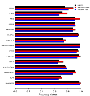
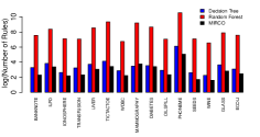
(a)    (b) (c)

Figure 3: (a) Accuracy values for RF, DT, and MIRCO. (b) Average percentage of missed samples by MIRCO. (c) Average number of rules (in logarithmic scale) generated by RF, DT, and MIRCO.

To compare RCB, we present the average accuracy values of RF, ADA, GB in Figure 4 (see Table S.3 for the details). We also report the results with the initial Decision Tree (iniDT) used in RCB algorithm (see line 2 in Algorithm 2) so that we can observe how rule generation improves performance. The number in parentheses above each dataset shows the average number of RMP calls by RCB. These results demosntrate that RCB exhibits a quite competitive performance. In particular, RCB outperforms both boosting algorithms, ADA and GB in four problems. One critical point here is that RCB makes only a small number of RMP calls. In all but one datasets, RCB improves the performance of the base decision tree, iniDT by using the proposed rule generation.

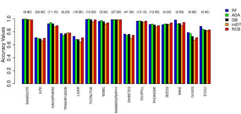
Figure 4: RCBoost results

5 Conclusion

We have proposed two algorithms for interpretation and boosting. Both algorithms are based on mathematical programming approaches for covering the rules in decision trees. The first algorithm is used for interpreting a model trained with the Random Forest algorithm. The second algorithm focuses on the idea of generating necessary rules to boost an initial model trained with the Decision Tree algorithm. Both algorithms are quite straightforward to implement within the existing packages. Even with our first implementation attempt, we have obtained promising results. The first algorithm has successfully extracted much less number of rules than the random forest model leading to better interpretability. Moreover, we have observed that the accuracy levels obtained with the extracted rules of our first algorithm closely follow the accuracy levels of the trained random forest model. When compared against other boosting algorithms, our second algorithm has shown a competitive performance. As a new boosting algorithm, we have also provided a discussion about the relationship between our approach and other boosting algorithms. The idea of selecting rules for interpretation or boosting leads to a plethora of extensions that could be further studied. Therefore, we have prepared a separate supplementary discussion on extensions in Section S.3. This section complements our discussion as well as lists several future research paths.

Note that most of the cross references in this supplementary file refer to the original manuscript. Therefore, clicking on those references may not take you to the desired location.

S.1 Chvatál’s greedy algorithm

We restate the well-known heuristic of Chvatál in our own notation. Recall that the sets $\mathcal{I}$ and $\mathcal{J}$ stand for the set of samples and the set of rules, respectively. Algorithm 3 gives the steps of the greedy heuristic, where $\mathcal{I}_{\mathcal{R}}(j)$ represents those samples that are in $\mathcal{R}$ covered by rule $j\in\mathcal{J}$. In line 3, the cost of selecting rule $j$ is $1+w_{j}$, and the operation $|\mathcal{I}_{\mathcal{R}}(j)|$ denotes the cardinality of the set $\mathcal{I}_{\mathcal{R}}(j)$. Removal of the redundant rules in line 3 is done in two steps: First, the rules in $\bar{\mathcal{J}}$ are sorted in ascending order of their costs in a list. Then, the rules at the end of this list are removed as long as the remaining rules cover all the samples.

Result: Set of rules $\hat{\mathcal{J}}$

1

2$\mathcal{R}=\mathcal{I}$, $\hat{\mathcal{J}}=\emptyset$;

3

4while $\mathcal{R}\neq\emptyset$ do

5      

6      $j^{*}=\arg\underset{j\in\mathcal{J}\backslash\hat{\mathcal{J}}}{\min}\left\{\frac{1+w_{j}}{|\mathcal{I}_{\mathcal{R}}(j)|}:\mathcal{I}_{\mathcal{R}}(j)\neq\emptyset\right\}$;

7      

8      $\mathcal{R}\leftarrow\mathcal{R}\backslash\mathcal{I}_{\mathcal{R}}(j^{*})$;

9      

10      $\hat{\mathcal{J}}\leftarrow\hat{\mathcal{J}}\cup j^{*}$;

11      

12 end while

13

14Remove redundant columns from $\hat{\mathcal{J}}$;

15

16Return $\hat{\mathcal{J}}$;

Algorithm 3 Greedy

S.2 Relation to other boosting algorithms

The use of sample weights and reduced costs shows a similar trait among RCBoost and other boosting algorithms. The reduced cost of rule $j$ can be considered as the partial derivative of the objective function with respect to the corresponding variable $z_{j}$. Thus, rules that have negative reduced costs are added to the rule pool. This resembles a descent iteration. To establish the relationship between RCBoost and other boosting methods from the gradient descent point of view [13], we first define the Lagrangean function

$$\mathcal{L}(\mathbf{z},\bm{\lambda})=\sum_{j\in\mathcal{J}}\big{(}1+w_{j}\big{)}z_{j}+\sum_{i\in\mathcal{I}}\lambda_{i}\big{(}1-\sum_{j\in\mathcal{J}(i)}z_{j}\big{)},$$

where $\mathbf{z}$ and $\bm{\lambda}$ denote the primal and dual vectors. Suppose that the optimal solution pair for (RMP$(\mathcal{J}_{t})$) is given by $\mathbf{z}^{t}$ and $\bm{\lambda}^{t}$. Then, we have

$$\begin{array}[]{rl}\mathcal{L}((\mathbf{z}^{t},\mathbf{z}^{c}),\bm{\lambda}^{t})&=\sum_{i\in\mathcal{I}}\lambda^{t}_{i}+\sum_{j\in\mathcal{J}_{t}}\bar{w}_{j}z^{t}_{j}+\sum_{j\in\mathcal{J}/\mathcal{J}_{t}}\bar{w}_{j}z^{t}_{j}\\[5.69054pt] &=\sum_{i\in\mathcal{I}}\lambda^{t}_{i}+\sum_{j\in\mathcal{J}/\mathcal{J}_{t}}\bar{w}_{j}z^{c}_{j},\end{array}$$

where $\bar{w}_{j}$ is the reduced cost of rule $j$ as in (4) and the tuple $(\mathbf{z}^{t},\mathbf{z}^{c})$ shows the variables in $\mathcal{J}_{t}$ and $\mathcal{J}/\mathcal{J}_{t}$, respectively. The last equality is a direct consequence of optimality conditions, since $\mathbf{z}^{t}$ and $\bm{\lambda}^{t}$ are complementary solution vectors. Thus, taking the steepest descent step for $j\in\mathcal{J}/\mathcal{J}_{t}$ simply implies involving those rules with negative reduced costs in the next iteration. From this perspective, RCBoost is similar to gradient boosting algorithms. Nonetheless, unlike those algorithms RCBoost does not fit a weak-classifier but instead obtains a larger set $\mathcal{J}_{t+1}$ by adding a subset of rules with negative reduced costs (line 2 of Algorithm 2). Then, solving the linear programming problem over $\mathcal{J}_{t+1}$ yields the parameters $\mathbf{z}^{t+1}$ and $\bm{\lambda}^{t+1}$. Suppose we denote the optimal objective function of (RMP$(\mathcal{J}_{t})$) by $\Phi(\mathcal{J}_{t})$, which is the total impurity that we use to evaluate the training loss of our classifier. With each iteration we improve this loss, since $\Phi(\mathcal{J}_{t})\geq\Phi(\mathcal{J}_{t+1})$ due to our linear programming formulation. If we further define the subset

$$\partial\mathcal{J}_{t}\subseteq\{j\in\mathcal{J}:\bar{w}_{j}<0\},$$

then $\Phi(\mathcal{J}_{t+1})=\Phi(\mathcal{J}_{t}\cup\partial\mathcal{J}_{t})$.

There has also been a focus on the margin maximization idea to discuss the generalization performance of boosting methods [14, 17]. Here, one of the fundamental points is to observe that a sample with a large margin is likely to be classified correctly. Thus, margin maximization is about assigning larger weights to those samples with small margins. RCBoost also implicitly aims at obtaining large margins through selection of rules with less impurities (classification errors decrease). In other words, minimizing the objective function of the restricted master problem promotes large margins. Formally, we can rewrite the optimal objective function value of (RMP$(\mathcal{J}_{t})$) as

$$\sum_{j\in\mathcal{J}_{t}}(1+w_{j})z^{t}_{j}=\sum_{i\in\mathcal{I}}\sum_{j\in\mathcal{J}_{t}(i)}\mu_{j}z^{t}_{j}=\sum_{i\in\mathcal{I}}\lambda_{i}^{t},$$

where $\mu_{j}=\frac{1+w_{j}}{|\mathcal{I}(j)|}$, $j\in\mathcal{J}$. Using complementary slackness condition, we know that $\lambda_{i}^{t}>0$ only if $\sum_{j\in\mathcal{J}_{t}(i)}z_{j}^{t}=1$. Thus, $\sum_{j\in\mathcal{J}_{t}(i)}\mu_{j}z^{t}_{j}$ is the convex combination of margins obtained with different rules for sample $i$. The larger the obtained impurity, the smaller the corresponding margin. Like other boosting methods, RCBoost also assigns larger weights to those samples with smaller margins.

S.3 Some extensions

We have used classification for our presentation. Nonetheless, both proposed algorithms can also be adjusted to solve regression problems. To interpret random forest regressors with MIRCO, the first step is to use a proper criterion, like mean squared error, for evaluating $w_{j}$, $j\in\mathcal{J}$ values. Then, MIRCO can be used as it is given in Algorithm 1. The same criteria can also be used in RCBoost to construct the restricted master problem. When a regression problem is solved, one needs to pay attention to two potential caveats: (i) The two components of the objective function coefficients in optimization model (1) or (3) may not be balanced well, since the criteria values $w_{j}$, $j\in\mathcal{J}$ are not bounded above by one. This could be overcome by scaling the criteria values. If scaling is done with a multiplier, then this multiplier becomes a new hyperparameter which may require tuning. (ii) Regression trees tend to have too many leaves. Even after applying MIRCO, the cardinality of the resulting set of rules $\hat{\mathcal{J}}$ may be quite large, and hence, interpreting the random forest regressor may be difficult. Similarly, RCBoost may make too many calls to the restricted master problem and end up with a large number of rules in the final rule pool $\mathcal{J}^{*}$.

Many boosting algorithms use decision trees as their weak estimators. Thus, it seems that MIRCO can also be used with those algorithms to interpret their results. However, one needs to pay attention to the fact that boosting algorithms assign different weights to their weak estimators and MIRCO does not take these weights into account. Therefore, if rule covering is used for interpretation of boosting algorithms, Algorithm 1 should be adjusted to incorporate the estimator weights.

Recall that we use a decision tree with sample weights in RCBoost as a proxy to an actual pricing subproblem (line 2, Algorithm 2). An alternative could be using the impurity and the negative reduced cost together while constructing the decision tree. In that case, splitting can be done from non-dominated bi-criteria values; i.e., impurity and negative reduced cost values.

Clearly, we can also use a random forest or any ensemble of trees with sample weights as a proxy to the pricing subproblem. Even further, one may even model a separate combinatorial problem to generate many different rules. At this point, it is important to keep in mind that considering all possible rules with negative reduced costs could prove to be a daunting job.

In its current stage, RCBoost adds all the rules with negative reduced costs to the rule pool. An alternative approach could be to include only the rule with the most negative reduced cost. Along the same vein, we may also remove those rules that have high (positive) reduced costs from the column pool. Actually, these are typical approaches in column generation to keep the size of the column pool manageable. As the size of the rule pool becomes large, RCBoost also becomes less interpretable. Fortunately, one can easily apply MIRCO or other rule extraction approaches from the literature such as the RuleFit algorithm [9] to a trained RCBoost. In that case, Algorithm 1 can be applied starting from line 1 with $\mathcal{J}\leftarrow\mathcal{J}^{*}$. As a final remark, we note that RCBoost treats the rules equally when a test point is classified with the satisfied rules in $\mathcal{J}^{*}$. An alternative could be giving different weights to different rules. These rule weights could be evaluated by making use of the optimal values of $z_{j}$, $j\in\mathcal{J}^{*}$ obtained from the final restricted master problem. However, all these changes should be carefully contemplated, since the resulting rule pool after shrinking may not necessarily cover the feature space as we have discussed in Section 2 (see also Figure 1).

S.4 Details of numerical results

Table S.1: Characteristics of the datasets

	Number of	Number of	Number of
Dataset	Features	Classes	Samples
banknote	4	2	1372
ILDP	10	2	583
ionosphere	34	2	351
transfusion	4	2	748
liver	6	2	345
tic-tac-toe	9	2	958
WDBC	30	2	569
mammography	6	2	11183
diabetes	8	2	768
oilspill	48	2	937
phoneme	5	2	5427
seeds	7	3	210
wine	13	3	178
glass	10	6	214
ecoli	7	8	336

Table S.2: MIRCO results

	DT	RF	MIRCO
Dataset	Accuracy	Accuracy	Accuracy	% of Missed Pts
banknote	0.99 (0.02)	0.99 (0.01)	0.98 (0.01)	0.01 (0.01)
ILDP	0.66 (0.07)	0.71 (0.06)	0.69 (0.03)	0.06 (0.04)
ionosphere	0.87 (0.07)	0.92 (0.03)	0.91 (0.04)	0.02 (0.03)
transfusion	0.79 (0.04)	0.77 (0.04)	0.76 (0.01)	0.01 (0.01)
liver	0.65 (0.09)	0.73 (0.06)	0.66 (0.06)	0.06 (0.05)
tic-tac-toe	0.94 (0.02)	0.99 (0.01)	0.97 (0.02)	0.02 (0.02)
WDBC	0.93 (0.03)	0.96 (0.02)	0.95 (0.03)	0.01 (0.02)
mammography	0.98 (0.00)	0.99 (0.00)	0.98 (0.00)	0.00 (0.00)
diabetes	0.74 (0.04)	0.77 (0.04)	0.73 (0.04)	0.05 (0.04)
oilspill	0.96 (0.02)	0.96 (0.01)	0.96 (0.01)	0.01 (0.01)
phoneme	0.88 (0.01)	0.91 (0.01)	0.88 (0.02)	0.03 (0.01)
seeds	0.91 (0.06)	0.91 (0.09)	0.91 (0.05)	0.02 (0.03)
wine	0.91 (0.07)	0.98 (0.03)	0.91 (0.07)	0.04 (0.04)
glass	0.67 (0.05)	0.79 (0.07)	0.71 (0.07)	0.09 (0.06)
ecoli	0.81 (0.09)	0.88 (0.06)	0.76 (0.08)	0.03 (0.03)
∗ Numbers in parantheses show the standard deviations

Table S.3: RCBoost results

	RF	ADA	GB	iniDT	RCB
Dataset	Accuracy	Accuracy	Accuracy	Accuracy	Accuracy
banknote	0.99 (0.01)	1.00 (0.00)	0.99 (0.01)	0.99 (0.01)	0.98 (0.01)
ILDP	0.71 (0.06)	0.70 (0.06)	0.69 (0.03)	0.66 (0.07)	0.70 (0.04)
ionosphere	0.92 (0.03)	0.94 (0.05)	0.92 (0.04)	0.88 (0.03)	0.89 (0.05)
transfusion	0.77 (0.04)	0.74 (0.04)	0.77 (0.03)	0.78 (0.03)	0.78 (0.04)
liver	0.73 (0.06)	0.68 (0.07)	0.68 (0.06)	0.64 (0.10)	0.71 (0.05)
tic-tac-toe	0.99 (0.01)	1.00 (0.01)	0.99 (0.01)	0.95 (0.02)	0.99 (0.01)
WDBC	0.96 (0.02)	0.97 (0.03)	0.96 (0.03)	0.92 (0.03)	0.94 (0.02)
mammography	0.99 (0.00)	0.99 (0.00)	0.99 (0.00)	0.98 (0.00)	0.99 (0.00)
diabetes	0.77 (0.04)	0.74 (0.04)	0.76 (0.04)	0.70 (0.06)	0.75 (0.03)
oilspill	0.96 (0.01)	0.97 (0.01)	0.96 (0.02)	0.95 (0.02)	0.96 (0.02)
phoneme	0.91 (0.01)	0.92 (0.01)	0.91 (0.01)	0.88 (0.01)	0.90 (0.01)
seeds	0.91 (0.09)	0.92 (0.07)	0.92 (0.07)	0.91 (0.09)	0.94 (0.06)
wine	0.98 (0.03)	0.92 (0.08)	0.93 (0.05)	0.89 (0.07)	0.94 (0.04)
glass	0.79 (0.07)	0.77 (0.08)	0.73 (0.10)	0.67 (0.11)	0.71 (0.09)
ecoli	0.88 (0.06)	0.84 (0.07)	0.83 (0.06)	0.82 (0.09)	0.83 (0.05)
∗ Numbers in parantheses show the standard deviations

References

- Bertsimas and Dunn [2017] D. Bertsimas and J. Dunn. Optimal classification trees. Machine Learning, 106(7):1039–1082, 2017.
- Breiman [2001] L. Breiman. Random forests. Machine Learning, 45(1):5–32, 2001.
- Chvatal [1979] V. Chvatal. A greedy heuristic for the set-covering problem. Mathematics of Operations Research, 4(3):233–235, 1979.
- Dash et al. [2018] S. Dash, O. Gunluk, and D. Wei. Boolean decision rules via column generation. In S. Bengio, H. Wallach, H. Larochelle, K. Grauman, N. Cesa-Bianchi, and R. Garnett, editors, Advances in Neural Information Processing Systems, pages 4655–4665. 2018.
- Demiriz et al. [2002] A. Demiriz, K. P. Bennett, and J. Shawe-Taylor. Linear programming boosting via column generation. Machine Learning, 46(1-3):225–254, 2002.
- Firat et al. [2020] M. Firat, G. Crognier, A. F. Gabor, C. Hurkens, and Y. Zhang. Column generation based heuristic for learning classification trees. Computers & Operations Research, 116:104866, 2020.
- Freund and Schapire [1997] Y. Freund and R. E. Schapire. A decision-theoretic generalization of on-line learning and an application to boosting. Journal of Computer and System Sciences, 55(1):119 – 139, 1997.
- Friedman [2001] J. H. Friedman. Greedy function approximation: A gradient boosting machine. Annals of Statistics, 29(5):1189–1232, 2001.
- Friedman and Popescu [2008] J. H. Friedman and B. E. Popescu. Predictive learning via rule ensembles. The Annals of Applied Statistics, 2(3):916–954, 2008.
- Günlük et al. [2018] O. Günlük, J. Kalagnanam, M. Menickelly, and K. Scheinberg. Optimal decision trees for categorical data via integer programming. arXiv preprint arXiv:1612.03225, 2018.
- Mashayekhi and Gras [2015] M. Mashayekhi and R. Gras. Rule extraction from random forest: the rf+hc methods. In D. Barbosa and E. Milios, editors, Advances in Artificial Intelligence, pages 223–237, Cham, 2015. Springer International Publishing.
- Mashayekhi and Gras [2017] M. Mashayekhi and R. Gras. Rule extraction from decision trees ensembles: New algorithms based on heuristic search and sparse group lasso methods. International Journal of Information Technology & Decision Making, 16(06):1707–1727, 2017.
- Mason et al. [1999] L. Mason, J. Baxter, P. Bartlett, and M. Frean. Boosting algorithms as gradient descent. In S. Solla, T. Leen, and K. Müller, editors, Advances in Neural Information Processing Systems, pages 512–518. 1999.
- Mason et al. [2000] L. Mason, , P. L. Bartlett, and J. Baxter. Improved generalization through explicit optimization of margins. Machine Learning, 38:243–255, 2000.
- Meinshausen [2010] N. Meinshausen. Node harvest. The Annals of Applied Statistics, 4(4):2049–2072, 2010.
- Pfetsch and Pokutta [2020] M. E. Pfetsch and S. Pokutta. IPBoost–non-convex boosting via integer programming. arXiv preprint arXiv:2002.04679, 2020.
- Schapire et al. [1998] R. E. Schapire, Y. Freund, P. Bartlett, and W. S. Lee. Boosting the margin: A new explanation for the effectiveness of voting methods. The Annals of Statistics, 26(5):1651–1686, 1998.
- Vasko et al. [2016] F. J. Vasko, Y. Lu, and K. Zyma. What is the best greedy-like heuristic for the weighted set covering problem? Operations Research Letters, 44:366–369, 2016.
Supplementary Material for