Fast approximation by periodic kernel-based lattice-point interpolation with application in uncertainty quantification

Abstract

This paper deals with the kernel-based approximation of a multivariate periodic function by interpolation at the points of an integration lattice—a setting that, as pointed out by Zeng, Leung, Hickernell (MCQMC2004, 2006) and Zeng, Kritzer, Hickernell (Constr. Approx., 2009), allows fast evaluation by fast Fourier transform, so avoiding the need for a linear solver. The main contribution of the paper is the application to the approximation problem for uncertainty quantification of elliptic partial differential equations, with the diffusion coefficient given by a random field that is periodic in the stochastic variables, in the model proposed recently by Kaarnioja, Kuo, Sloan (SIAM J. Numer. Anal., 2020). The paper gives a full error analysis, and full details of the construction of lattices needed to ensure a good (but inevitably not optimal) rate of convergence and an error bound independent of dimension. Numerical experiments support the theory.

1 Introduction

We consider a kernel-based approximation for a multivariate periodic function by interpolation at a quasi-Monte Carlo lattice point set. Kernel-based interpolation methods are by now well established (see, e.g., [26] and more discussion below). It is the unique combination of a periodic kernel plus a lattice point set here that will deliver us the significant advantage in computational efficiency. As already advocated by Hickernell and colleagues in [28, 29], the combination of a periodic reproducing kernel with the group structure of lattice points means that the linear system for constructing the kernel interpolant involves a circulant matrix, thus can be solved very efficiently using the fast Fourier transform. So, our kernel method can be fast even if the dimensionality is high.

As also advocated in [28, 29], a kernel interpolant is in many settings optimal among all approximation algorithms that use the same function values (see also known results on optimal recovery, e.g., [20, 21]). We can therefore analyze the worst case approximation error of our kernel method by using, as upper bound, the worst case error of an auxiliary algorithm based on a Fourier series truncated at a hyperbolic cross index set. Using recent works [3, 4], we here construct a lattice generating vector with a guaranteed good error bound for our kernel interpolant. Note, importantly, that neither the construction of our lattice generating vector, nor the implementation of our kernel method, requires explicit knowledge or evaluation of the auxiliary hyperbolic cross index set. In short, we know how to find a good lattice point set so that our kernel method has a small error in addition to being of low cost.

In this paper, the main contribution is to apply and analyze this periodic-kernel-plus-lattice method to uncertainty quantification of elliptic partial differential equations (PDEs), where the diffusion coefficient is given by a random field that is periodic in the stochastic variables, as in the model proposed recently by Kaarnioja, Kuo, and Sloan [12]. We tailor our lattice generating vector to the regularity of the PDE solution with respect to the stochastic variables. Our numerical results beat the theoretical predictions, indicating that the theory based on worst case analysis may not be sharp.

The kernel approximation developed here may have a role as a surrogate model for complicated forward problems. One popular use for surrogate models is to allow efficient sampling of the original system. If the solution of some particularly difficult PDE problem with high accuracy takes a week for a given parameter choice $\boldsymbol{y}$, then having a kernel interpolant that can be evaluated in hours or minutes could be very useful. A second possible use for the kernel interpolant is in the easy generation of derivatives, needed for example in gradient-based optimization algorithms. The surrogate might be even more useful for Bayesian inverse problems.

We now elaborate key points.

Periodic-kernel-plus-lattice method. Let $f(\boldsymbol{y})=f(y_{1},\ldots,y_{s})$ be a real-valued function on the $s$-dimensional unit cube $[0,1]^{s}$, with a somewhat smooth 1-periodic extension to ${\mathbb{R}}^{s}$. Our main interest is in problems where the dimension $s$ is large. Following [25], we assume that $f$ has an absolutely convergent Fourier series, and belongs to a weighted mixed Sobolev space $H:=H_{s,\alpha,{\boldsymbol{\gamma}}}$ which is characterized by a smoothness parameter $\alpha>1$ and a family of positive numbers ${\boldsymbol{\gamma}}=(\gamma_{\mathfrak{u}})_{{\mathfrak{u}}\subset{\mathbb{N}}}$ called weights; the details are given in Section 2.1.

Our ultimate application, to be analyzed in Section 4, concerns a class of elliptic PDEs parameterized by a very high (or possibly countably infinite) number of stochastic parameters, for which the solution, as a function of the parameters, is periodic and belongs to the weighted space $H$ for a suitable choice of $\alpha$ and ${\boldsymbol{\gamma}}$.

The important feature of the space $H$ is that it is a reproducing kernel Hilbert space (RKHS), with a simple reproducing kernel $K(\boldsymbol{y},\boldsymbol{y}^{\prime})$. This opens the way to the use of kernel methods to approximate functions in $H$ from given point values. In particular, in this paper we focus on the kernel interpolation: given $f\in H$ and a suitable set of points ${\boldsymbol{t}}_{1},\dots,{\boldsymbol{t}}_{n}\in[0,1]^{s}$, we seek for an approximation $f_{n}\in H$ of the form

$$f_{n}(\boldsymbol{y})\,:=\,\sum_{k=1}^{n}a_{k}\,K({\boldsymbol{t}}_{k},\boldsymbol{y}),\qquad\boldsymbol{y}\in[0,1)^{s},$$ (1)

which satisfies the interpolation condition $f_{n}({\boldsymbol{t}}_{k})=f({\boldsymbol{t}}_{k})$, $k=1,\dots,n$. We refer to $f_{n}$ as the kernel interpolant of $f$.

We will interpolate the function at a set of $n$ lattice points specified by a generating vector ${\boldsymbol{z}}\in{\mathbb{Z}}^{s}$. The points are then given by the formula ${\boldsymbol{t}}_{k}={(k{\boldsymbol{z}}\bmod n)/{n}}$, $k=1,\ldots,n$, with ${\boldsymbol{t}}_{n}={\boldsymbol{t}}_{0}=\boldsymbol{0}$. A lattice point set has an additive group structure, implying that the difference of two lattice points is another lattice point (after taking into account periodicity).

A key property of our reproducing kernel is that it depends only on the difference of the two arguments, thus $K(\boldsymbol{y},\boldsymbol{y}^{\prime})=K(\boldsymbol{y}-\boldsymbol{y}^{\prime},\boldsymbol{0})$, and $K(\cdot,\boldsymbol{0})$ is a periodic function with an easily computable expression when $\alpha$ is an even integer. Combining this with the group structure of lattice points means that the matrix $[K({\boldsymbol{t}}_{k}-{\boldsymbol{t}}_{k^{\prime}},\boldsymbol{0})]_{k,k^{\prime}=1,\ldots,n}$ contains only $n$ distinct values and indeed is a circulant matrix. Therefore the linear system arising from collocating (1) at the points ${\boldsymbol{t}}_{k^{\prime}},k^{\prime}=1,\ldots,n$, can be solved using the fast Fourier transform with a cost of ${\mathcal{O}}(n\log(n))$.

Once we have the coefficients $a_{k}$, we can use (1) to evaluate the interpolant $f_{n}$ at $L$ arbitrary points $\boldsymbol{y}_{\ell}$, $\ell=1,\ldots,L$, with a cost of ${\mathcal{O}}(Ln)$. Remarkably, with almost the same cost we can evaluate $f_{n}$ at all the $Ln$ points of the union of shifted lattices $\boldsymbol{y}_{\ell}+{\boldsymbol{t}}_{k^{\prime}}$, $\ell=1,\ldots,L$, $k^{\prime}=1,\ldots,n$. Indeed, since $K({\boldsymbol{t}}_{k},\boldsymbol{y}_{\ell}+{\boldsymbol{t}}_{k^{\prime}})=K({\boldsymbol{t}}_{k}-{\boldsymbol{t}}_{k^{\prime}},\boldsymbol{y}_{\ell})$ and the matrix $[K({\boldsymbol{t}}_{k}-{\boldsymbol{t}}_{k^{\prime}},\boldsymbol{y}_{\ell})]_{k,k^{\prime}=1,\ldots,n}$ is circulant, we have

$$f_{n}(\boldsymbol{y}_{\ell}+{\boldsymbol{t}}_{k^{\prime}})\,=\,\sum_{k=1}^{n}a_{k}\,K({\boldsymbol{t}}_{k}-{\boldsymbol{t}}_{k^{\prime}},\boldsymbol{y}_{\ell}),$$

which can be evaluated for each $\boldsymbol{y}_{\ell}$ for all ${\boldsymbol{t}}_{k^{\prime}}$ together by fast Fourier transform with a cost of ${\mathcal{O}}(n\log(n))$, leading to the total cost of ${\mathcal{O}}(Ln\log(n))$. Comprehensive cost analysis taking into account also the evaluations of $f$ and $K$ is given in Section 5.

Brief survey on kernel methods in high dimensions. Griebel and Rieger [10] considered a (non-interpolatory) kernel approximation based on a regularized reconstruction technique from machine learning for a class of parameterized elliptic PDEs similar to the one considered in this work, yet with non-periodic dependence on the parameters. They used an anisotropic kernel, behaving differently in different variables, to address the high dimensionality of the problem. However, their error estimate was in terms of the mesh norm or fill distance of the point set, which is the Euclidean radius of the largest Euclidean ball that contains no points in its interior. Since the fill distance behaves at best like $n^{-1/s}$, where $n$ is the number of sampling points, their estimates inevitably suffer the curse of dimensionality.

Kempf et al. [15] considered the same PDE problem and anisotropic kernel as [10]. However, they considered a penalized least-squares approach for kernel approximation and an isotropic sparse grid as point set, which allowed them to obtain error estimates with a mitigated (but still present) curse of dimensionality.

As noted above, lattice points have already been used in a kernel interpolation method. Zeng et al. [28] seem to be the first to work in this direction, however the question of dependence on dimension was not considered in their analysis. Zeng et al. [29] established dimension independent error estimates in weighted spaces in the case of product weights (i.e., weights that have the form $\gamma_{{\mathfrak{u}}}=\prod_{j\in{\mathfrak{u}}}\gamma_{j}$). We note, however, that the assumption of product weights is rather limiting. For instance, for integration problems involving parameterized PDEs, the best convergence rates known up to now are obtained by considering weighted space for the parameter-to-solution map with (S)POD weights [9, 12, 17], whereas weighted spaces with product weights lead to the best known rates only for special models [7, 11, 14]. In this paper we extend these results to the case of kernel approximation (as opposed to integration) of the parameter-to-solution map, and we are able to show dimension-independent convergence rates using (S)POD weights in the general case. To the best of our knowledge, this is the first paper to use non-product weights for approximation in parameterized PDE problems.

PDEs with periodic dependence on random variables. Our motivating application is a class of parameterized elliptic PDEs with periodic dependence on the parameters, for which we will establish dimension independent error estimate for the kernel interpolant, by deriving suitable choices of smoothness parameter and weights for the problem at hand. To the best of our knowledge, this is the first paper presenting dimension independent kernel approximation methods using lattice points for this class of problems.

We consider uncertainty quantification for an elliptic PDE (see details in Section 4) on a physical domain $D\subset\mathbb{R}^{d}$, $d=1,2$ or $3$, in a probability space $(\Omega,\mathscr{A},\mathbb{P})$, with an input random field of the form

$$a({\boldsymbol{x}},\omega)\,=\,a_{0}({\boldsymbol{x}})+\sum_{j\geq 1}\Theta_{j}(\omega)\,\psi_{j}({\boldsymbol{x}}),\qquad{\boldsymbol{x}}\in D,~{}\omega\in\Omega,$$

where $a_{0}$ and $\psi_{j}$ are uniformly bounded in $D$, and $\Theta_{j}(\omega)$ are i.i.d. random variables following a prescribed distribution. In the popular affine model, $\Theta_{j}$ are i.i.d. random variables uniformly distributed on $[-\frac{1}{2},\frac{1}{2}]$. In the periodic model [12], $\Theta_{j}$ are i.i.d. random variables distributed according to the arcsine distribution and can be parameterized as

$$\Theta_{j}\,=\,\frac{1}{\sqrt{6}}\sin(2\pi y_{j}),\qquad j\geq 1,$$

with $y_{j}$ uniformly distributed on $[-\frac{1}{2},\frac{1}{2}]$. The mean of the random field is $a_{0}$, and the scaling ${{1}/{\sqrt{6}}}$ is chosen here so that the covariance of the random field is also exactly the same as in the affine case. Higher moments are of course somewhat different, but as argued in [12], there seems to be no clear reason for preferring one over the other.

Due to periodicity, it is equivalent to work with $y_{j}$ uniformly distributed in the interval $[0,1]$ instead of $[-\frac{1}{2},\frac{1}{2}]$, thus from now on we consider the parameter space

$$\boldsymbol{y}\in U\,:=\,[0,1]^{\mathbb{N}}.$$

In the earlier paper [12] the aim was to develop and analyze a method for computing the expected value of a given quantity of interest, expressed as a linear functional of the PDE solution, hence facing a high dimensional integration problem. Here, in contrast, the aim is to develop and analyze a fast method for approximating the solution $u({\boldsymbol{x}},\boldsymbol{y})$, or some quantity of interest $Q(\boldsymbol{y})$ derived from $u({\boldsymbol{x}},\boldsymbol{y})$, as an explicit function of $\boldsymbol{y}$. To that end we will develop a kernel-based approximation, using the kernel of a reproducing kernel Hilbert space of periodic functions, and interpolation at a lattice point set.

Structure of the paper. In Section 2 we define the function space setting and the kernel interpolant, and establish its principal properties, while giving a simple proof of a known optimality result, namely that in the sense of worst case error the kernel interpolant is an optimal $L_{p}$ approximation among all approximations that use the same information about the target function $f\in H$. Then in Section 3 we establish upper and lower bounds on the error. For the upper bound we use the optimality result together with the error analysis for a trigonometric polynomial method established by two of the current authors together with Cools and Nuyens [3, 4]. For the lower bound we provide another proof of a recent result by Byrenheid et al. [1], namely that a method that draws information only from function values at lattice points inevitably has a rate of convergence that is at best only half of the best possible rate, thereby obtaining matching upper and lower bounds up to logarithmic factors. In Section 4, we apply the error analysis developed in Section 3 to a parameterized PDE problem, thereby obtaining rigorous upper error bounds that are independent of dimension and have explicit rates of convergence. Section 5 is concerned with the cost analysis of our proposed method. In Section 6 we give the results of some numerical experiments.

2 The kernel interpolant

2.1 The function space setting

Let $f(\boldsymbol{y})=f(y_{1},\ldots,y_{s})$ be a real-valued function on $[0,1]^{s}$ with a somewhat smooth $1$-periodic extension to $\mathbb{R}^{s}$ with respect to each variable $y_{j}$. Our main interest is in problems where the dimension $s$ is large. Following [25], we assume that $f$ has absolutely convergent Fourier series (and so is continuous),

$$f(\boldsymbol{y})\,=\,\sum_{{\boldsymbol{h}}\in{\mathbb{Z}}^{s}}\widehat{f}({\boldsymbol{h}})\,{\mathrm{e}}^{2\pi{\mathrm{i}}{\boldsymbol{h}}\cdot\boldsymbol{y}},\qquad\mbox{with}\qquad\widehat{f}({\boldsymbol{h}}) \,:=\,\int_{[0,1]^{s}}f(\boldsymbol{y})\,\rm{e}^{-2\pi{\mathrm{i}}{\boldsymbol{h}}\cdot\boldsymbol{y}}\,{\mathrm{d}}\boldsymbol{y};$$

and moreover belongs to a weighted mixed Sobolev space $H:=H_{s,\alpha,{\boldsymbol{\gamma}}}$, a Hilbert space with inner product and norm

$$\langle f,g\rangle_{H} \,:=\,\langle f,g\rangle_{s,\alpha,{\boldsymbol{\gamma}}}\,:=\,\sum_{{\boldsymbol{h}}\in{\mathbb{Z}}^{s}}r({\boldsymbol{h}})\,\widehat{f}({\boldsymbol{h}})\,\overline{\widehat{g}({\boldsymbol{h}})},$$

$$\|f\|_{H} \,:=\,\|f\|_{s,\alpha,{\boldsymbol{\gamma}}}\,:=\,\bigg{(}\sum_{{\boldsymbol{h}}\in{\mathbb{Z}}^{s}}r({\boldsymbol{h}})\,|\widehat{f}({\boldsymbol{h}})|^{2}\bigg{)}^{1/2},$$

where

$$r({\boldsymbol{h}})\,:=\,r_{s,\alpha,{\boldsymbol{\gamma}}}({\boldsymbol{h}})\,:=\,\frac{1}{\gamma_{{\mathrm{supp}}({\boldsymbol{h}})}}\prod_{j\in{\mathrm{supp}}({\boldsymbol{h}})}|h_{j}|^{\alpha},$$

with ${\mathrm{supp}}({\boldsymbol{h}}):=\left\{j\in\{1:s\}:h_{j}\neq 0\right\}$ and $\{1:s\}:=\{1,2,\ldots,s\}$, and with the ${\boldsymbol{h}}=\boldsymbol{0}$ term in the sum to be interpreted as $\gamma_{\emptyset}^{-1}|\widehat{f}(\boldsymbol{0})|^{2}$. The weighted space $H_{s,\alpha,{\boldsymbol{\gamma}}}$ is characterized by the smoothness parameter $\alpha>1$ and a family of positive numbers ${\boldsymbol{\gamma}}=(\gamma_{\mathfrak{u}})_{{\mathfrak{u}}\subset{\mathbb{N}}}$ called weights, where a positive weight $\gamma_{\mathfrak{u}}$ is associated with each subset ${\mathfrak{u}}\subseteq\{1:s\}$. We fix the scaling of the weights by setting $\gamma_{\emptyset}:=1$, so that the norm of a constant function in $H$ matches its $L_{2}$ norm.

It can easily be verified that if $\alpha$ is an even integer then the norm can be rewritten as the norm in an “unanchored” weighted Sobolev space of dominating mixed smoothness of order ${{\alpha}/{2}}$,

$$\|f\|_{H}=\sqrt{\sum_{{\mathfrak{u}}\subseteq\{1:s\}}\frac{1}{(2\pi)^{\alpha|{\mathfrak{u}}|}\gamma_{\mathfrak{u}}}\int_{[0,1]^{|{\mathfrak{u}}|}}\!\!\;\bigg{|}\int_{[0,1]^{s-|{\mathfrak{u}}|}}\bigg{(}\prod_{j\in{\mathfrak{u}}}\frac{\partial^{\alpha/2}}{\partial y_{j}^{\alpha/2}}\bigg{)}f(\boldsymbol{y})\,{\mathrm{d}}\boldsymbol{y}_{-{\mathfrak{u}}}\bigg{|}^{2}\,{\mathrm{d}}\boldsymbol{y}_{\mathfrak{u}}},$$ (2)

where $\boldsymbol{y}_{\mathfrak{u}}$ denotes the components of $\boldsymbol{y}$ with indices that belong to the subset ${\mathfrak{u}}$, and $\boldsymbol{y}_{-{\mathfrak{u}}}$ denotes the components that do not belong to ${\mathfrak{u}}$, and $|{\mathfrak{u}}|$ denotes the cardinality of ${\mathfrak{u}}$.

The important feature of the space $H$ is that it is an RKHS, with an explicitly known and analytically simple reproducing kernel, namely

$$K(\boldsymbol{y},\boldsymbol{y}^{\prime})\,:=\,K_{s,\alpha,{\boldsymbol{\gamma}}}(\boldsymbol{y},\boldsymbol{y}^{\prime})\,:=\,\sum_{{\mathfrak{u}}\subseteq{\{1:s\}}}\gamma_{{\mathfrak{u}}}\prod_{j\in{\mathfrak{u}}}\eta_{\alpha}(y_{j},y_{j}^{\prime}),$$

where

$$\eta_{\alpha}(y,y^{\prime})\,:=\,\eta_{\alpha}(y-y^{\prime})\,:=\,\sum_{h\neq 0}\frac{{\mathrm{e}}^{2\pi{\mathrm{i}}h(y-y^{\prime})}}{|h|^{\alpha}}\,=\,\sum_{h\neq 0}\frac{\cos{2\pi h(y-y^{\prime})}}{|h|^{\alpha}}.$$

Note that the reproducing property

$$\langle f,K(\cdot,\boldsymbol{y})\rangle_{H}\,=\,f(\boldsymbol{y})\qquad\mbox{for all $f\in H$ and all $\boldsymbol{y}\in[0,1]^{s}$},$$ (3)

is easily verified.

Of special interest are even integer values of $\alpha$, because, when $\alpha$ is even, $\eta_{\alpha}$ can be expressed in the especially simple closed form

$$\eta_{\alpha}(y,y^{\prime})\,=\,\frac{(2\pi)^{\alpha}}{(-1)^{\alpha/2+1}\alpha!}B_{\alpha}(\{y-y^{\prime}\}),\qquad y,y^{\prime}\in[0,1],$$

where the braces indicate that $y-y^{\prime}$ is to be replaced by its fractional part in $[0,1)$, and $B_{\alpha}(y)$ is the Bernoulli polynomial of degree $\alpha$. For example, for $\alpha=2$ and $\alpha=4$ we have

$$B_{2}(y)\,=\,y^{2}-y+\frac{1}{6}\qquad\mbox{and}\qquad B_{4}(y)\,=\,y^{4}-2y^{3}+y^{2}-\frac{1}{30}.$$

2.2 The kernel interpolant

We are interested in approximating a given function $f\in H$ by an approximation of the form

$$A^{*}_{n}(f):=f_{n}(\boldsymbol{y}):=f_{s,\alpha,{\boldsymbol{\gamma}},n,{\boldsymbol{z}}}(\boldsymbol{y}):=\sum_{k=1}^{n}a_{k}\,K\Big{(}\Big{\{}\frac{k{\boldsymbol{z}}}{n}\Big{\}},\boldsymbol{y}\Big{)},\qquad\boldsymbol{y}\in[0,1)^{s},$$ (4)

where ${\boldsymbol{z}}\in\{1,\dots,n-1\}^{s}$, and the braces around the vector of length $s$ indicate that each component of the vector is to be replaced by its fractional part. The points

$${\boldsymbol{t}}_{k}\,:=\,\Big{\{}\frac{k{\boldsymbol{z}}}{n}\Big{\}}\qquad\mbox{for}\qquad k=1,\dots,n$$ (5)

are the points of a lattice cubature rule of rank $1$, see [24]. In what follows, we omit these braces because functions we consider are, unless otherwise stated, periodic.

In particular, we define $f_{n}\in H$ to be the function of the form (4) that interpolates $f$ at the lattice points,

$$f_{n}({\boldsymbol{t}}_{k})\,=\,f({\boldsymbol{t}}_{k})\qquad\mbox{for all}\qquad k=1,\dots,n,$$ (6)

and refer to $f_{n}$ as the kernel interpolant of $f$.

The coefficients $a_{k}$ in (4) are given by the linear system based on (6)

$$\sum_{k=1}^{n}{\mathcal{K}}_{k,k^{\prime}}\,a_{k}\,=\,f\left({\boldsymbol{t}}_{k^{\prime}}\right)\qquad\mbox{for all}\qquad k^{\prime}=1,\dots,n,$$ (7)

where ${\mathcal{K}}_{k^{\prime},k}\,=\,{\mathcal{K}}_{k,k^{\prime}}\,:=\,K({\boldsymbol{t}}_{k},{\boldsymbol{t}}_{k^{\prime}})$, $k,k^{\prime}=1,\ldots,n$. Note that the matrix elements can be expressed, using periodicity, as

$${\mathcal{K}}_{k,k^{\prime}}\,=\,K\biggl{(}{\frac{(k-k^{\prime}){\boldsymbol{z}}}{n}},\boldsymbol{0}\biggr{)},$$

where $\boldsymbol{0}$ is the $s$-vector of all zeroes. It follows that the $n\times n$ matrix ${\mathcal{K}}$ is a circulant matrix, which contains only $n$ distinct elements, and can be diagonalised in a time of order $n\log n$ by fast Fourier transform. This is a major motivation for using lattice points.

2.3 The kernel interpolant is the minimal norm interpolant

The following property is a well known result for interpolation in a reproducing kernel Hilbert space; for completeness we give a proof.

Theorem 1.

The kernel interpolant $f_{n}$ defined by (4), (5) and (6) is the minimal norm interpolant in $H$.

Proof.

Denoting the linear span of the kernels with one leg at ${\boldsymbol{t}}_{k},k=1,\ldots,n$ by

$$P_{n}\,:=\,\mathrm{span}\{K({\boldsymbol{t}}_{k},\cdot):k=1,\ldots,n\},$$

we observe the well known fact (see, e.g., [5, 8]), that $f_{n}$ is the orthogonal projection of $f$ on $P_{n}$ with respect to the inner product $\langle\cdot,\cdot\rangle_{H}$, since from the reproducing property (3) and the interpolation property (6) we have

$$\langle f-f_{n},K({\boldsymbol{t}}_{k},\cdot)\rangle_{H}\,=\,f({\boldsymbol{t}}_{k})-f_{n}({\boldsymbol{t}}_{k})\,=\,0\qquad\mbox{for all}\qquad k=1,\dots,n.$$

In turn, there follows the Pythagoras theorem,

$$\|f\|_{H}^{2}\,=\,\|f-f_{n}\|_{H}^{2}+\|f_{n}\|_{H}^{2},$$ (8)

and the minimal norm property of $f_{n}$,

$$f_{n}\,=\,\mathrm{argmin}\big{\{}\|g\|_{H}\;:\;g\in H\mbox{ and }g({\boldsymbol{t}}_{k})=f({\boldsymbol{t}}_{k})\mbox{ for all }k=1,\ldots,n\big{\}},$$

since if $g$ is any other interpolant of $f$ at the lattice points then

$$\langle g-f_{n},f_{n}\rangle_{H}\,=\,\sum_{k=1}^{n}a_{k}\,\langle g-f_{n},K({\boldsymbol{t}}_{k},\cdot)\rangle_{H}\,=\,0,$$

and hence $\|g\|_{H}^{2}\,=\,\|g-f_{n}\|_{H}^{2}+\|f_{n}\|_{H}^{2}$, from which the uniqueness of the minimal norm interpolant also follows. $\Box$

2.4 The kernel interpolant is optimal for given function values

In this subsection we show that the kernel interpolant $f_{n}$ defined by (4), (5) and (6) is optimal among all approximations that use only the same function values of $f$, in the sense of giving the least possible worst case error measured in any given norm $\|\cdot\|_{W}$ such that $H\subset W$ for functions in $H$. This is a special case of a general result for optimal recovery problems in Hilbert spaces (see for example [20, Example 1.1] and [21, Section 3]), but for completeness we give a short proof here. Our proof follows the exposition of [26, Proof of Theorem 13.5], but suitably adapted to our setting.

Let $A_{n}:H\to H$ be an algorithm (linear or non-linear) that uses as information about the argument only its values at the points (5), i.e., it is a mapping of the form $A_{n}(f)=\mathcal{I}_{n}(f({\boldsymbol{t}}_{1}),\dots,f({\boldsymbol{t}}_{n}))$ for a mapping $\mathcal{I}_{{n}}\colon\mathbb{R}^{n}\to H$. The worst case $W$-error for this algorithm is defined by

$$e^{\rm wor}(A_{n};W)\,:=\,\sup_{f\in H,\,\|f\|_{H}\leq 1}\|f-A_{n}(f)\|_{W}.$$

Theorem 2.

Let $A_{n}:H\to H$ be an algorithm (linear or non-linear) such that $A_{n}(f)$ uses as information about $f$ only its values $f({\boldsymbol{t}}_{1}),\ldots,f({\boldsymbol{t}}_{n})$ at the points (5). For $f\in H$, let $A^{*}_{n}(f):=f_{n}$ be the kernel interpolant defined by (4), (5) and (6). Then, for any normed space $W\supset H$ we have

$$e^{\rm wor}(A^{*}_{n};W)\,\leq\,e^{\rm wor}(A_{n};W).$$

Proof.

Define $\mathcal{C}:=\{g\in H\;:\;\|g\|_{H}\leq 1\text{ and }g({\boldsymbol{t}}_{k})=0\mbox{ for all }k=1,\ldots,n\}$. For any $g\in\mathcal{C}$ we have

$$\|g\|_{W} \leq\frac{1}{2}(\|g-A_{n}(0)\|_{W}+\|g+A_{n}(0)\|_{W})$$

$$\leq\max\big{(}\|g-A_{n}(0)\|_{W},\|g+A_{n}(0)\|_{W}\big{)}$$

$$=\max\big{(}\|g-A_{n}(g)\|_{W},\|(-g)-A_{n}(-g)\|_{W}\big{)}\leq e^{\rm wor}(A_{n};W),$$ (9)

where in the penultimate step we used $g({\boldsymbol{t}}_{k})=0$ for all $k=1,\ldots,n$, from which it follows that $A_{n}(0)=A_{n}(g)=A_{n}(-g)$. For any $f\in H$ such that $\|f\|_{H}\leq 1$, since $f_{n}$ is interpolatory, the Pythagoras theorem (8) implies $\|f-f_{n}\|_{H}\leq 1$, and hence $f-f_{n}\in\mathcal{C}$. Thus it follows from (2.4) that

$$\|f-A^{*}_{n}(f)\|_{W}\,=\,\|f-f_{n}\|_{W}\,\leq\,e^{\rm wor}(A_{n};W).$$

The theorem now follows. $\Box$

In the above result, we may, for example, take $W=L_{p}$ for any $1\leq p\leq\infty$.

3 Lower and upper error bounds

3.1 Lower bound on the worst case $L_{p}$ error ($1\leq p\leq\infty$)

A recent paper [1] showed (with a different definition of the parameter $\alpha$) that the worst case $L_{2}$ error for an approximation that uses the points of a rank-$1$ lattice cannot have an order of convergence better than $n^{-\alpha/4}$ (with our definition of $\alpha$). Bearing in mind that $H$ is a (Hilbert) space of functions of dominating mixed smoothness of order ${{\alpha}/{2}}$, this is just half the rate $n^{-\alpha/2}$ of the best approximation. Since the function space setting in that paper is rather different from ours (here we use a Fourier description and a so-called unanchored space, and have introduced weights) we briefly reprove the main result here, obtaining a sharp lower bound expressed in terms of the weights. Furthermore, in our setting we make the result stronger by showing that the same lower bound holds for the worse case $L_{1}$ error.

Theorem 3.

Let $s\geq 2$. Assume that the weights for the subsets of $\{1:s\}$ containing a single element satisfy ${\gamma_{\{j\}}}>0$ for all $j\in\{1:s\}$, and that ${\boldsymbol{z}}\in\{0,\ldots,n-1\}^{s}$ is given. Let $A_{n}:H\to L_{p}$ be an algorithm (linear or non-linear) that uses information only at the lattice points (5) and satisfies $A_{n}(0)=0$. Then for $1\leq p\leq\infty$ the worst case $L_{{p}}$ error for algorithm $A_{n}$ satisfies

$$e^{\rm wor}(A_{n};L_{{p}})\,\geq\,\sqrt{\frac{2}{1/\gamma_{\{{j}\}}+1/\gamma_{\{{k}\}}}}\,n^{-\alpha/4}\quad\text{ for any }j,k\in\{1:s\}\mbox{ with }j\neq k.$$

In particular, if $\gamma_{\{1\}}\geq\gamma_{\{2\}}\geq\dotsb>0$ then

$$e^{\rm wor}(A_{n};L_{p})\geq\sqrt{{{2}/{\big{(}\gamma_{\{1\}}^{-1}+\gamma_{\{2\}}^{-1}\big{)}}}}\,n^{-\alpha/4}.$$

Proof.

Without loss of generality we assume $\gamma_{\{1\}}\geq\gamma_{\{2\}}\geq\dotsb>0$. The heart of the matter is that there exists a non-zero integer vector ${\boldsymbol{h}}^{*}$ of length $s$ in the $2$-dimensional set

$$D_{n}\,:=\,\left\{(h_{1},h_{2},0,\ldots,0)\;:\;h_{j}\in\mathbb{Z},\,0\leq|h_{j}|\leq\lfloor\sqrt{n}\rfloor,\,j=1,2\right\},$$

such that

$${\boldsymbol{h}}^{*}\cdot{\boldsymbol{z}}\equiv 0\pmod{n}.$$ (10)

(In the language of dual lattices, see [24], there exists a point of the dual lattice in $D_{n}\setminus\{\boldsymbol{0}\}$.) To prove this fact, we define $\widetilde{D}_{n}$, the positive quadrant of $D_{n}$, by

$$\widetilde{D}_{n}\,:=\,\left\{(h_{1},h_{2},0,\ldots,0)\;\colon\;h_{j}\in\mathbb{Z},\,0\leq h_{j}\leq\lfloor\sqrt{n}\rfloor,\,j=1,2\right\},$$

noting that if ${\boldsymbol{h}},{\boldsymbol{h}}^{\prime}\in\widetilde{D}_{n}$ then ${\boldsymbol{h}}-{\boldsymbol{h}}^{\prime}\in D_{n}$. Now define

$$E_{n}({\boldsymbol{z}})\,:=\,\{({\boldsymbol{h}}\cdot{\boldsymbol{z}}\bmod n)\in\{0,\dots,n-1\}\ \colon\ {\boldsymbol{h}}\in\widetilde{D}_{n}\}.$$

Since $|E_{n}({\boldsymbol{z}})|\leq n$ and $|\widetilde{D}_{n}|=(1+\lfloor\sqrt{n}\rfloor)^{2}>n$, it follows from the pigeonhole principle that two distinct elements of $\widetilde{D}_{n}$, say ${\boldsymbol{h}}$ and ${\boldsymbol{h}}^{\prime}$, yield the same element of $E_{n}({\boldsymbol{z}})$; from this it follows that ${\boldsymbol{h}}^{*}:={\boldsymbol{h}}-{\boldsymbol{h}}^{\prime}$ satisfies (10). A “fooling function” is then defined by

$$q(\boldsymbol{y})\,:=\,\mathrm{e}^{2\pi\mathrm{i}h_{1}^{*}{\boldsymbol{e}}_{1}\cdot\boldsymbol{y}}-\mathrm{e}^{-2\pi\mathrm{i}h_{2}^{*}{\boldsymbol{e}}_{2}\cdot\boldsymbol{y}}\,=\,\mathrm{e}^{-2\pi\mathrm{i}h_{2}^{*}{\boldsymbol{e}}_{2}\cdot\boldsymbol{y}}\big{(}\mathrm{e}^{2\pi\mathrm{i}{\boldsymbol{h}}^{*}\cdot\boldsymbol{y}}-1\big{)},\qquad{\boldsymbol{y}\in\mathbb{R}^{s}},$$

where ${\boldsymbol{e}}_{1}$ and ${\boldsymbol{e}}_{2}$ are the unit vectors corresponding to variables $1$ and $2$. By construction, $q$ vanishes at all the lattice points (5). For this function, since the two terms in $q$ are orthogonal with respect to the inner products in $H=H_{s,\alpha,{\boldsymbol{\gamma}}}$, the squared $H$ norm satisfies

$$\|q\|_{H}^{2}=r(h_{1}^{*}{\boldsymbol{e}}_{1})+{r}(-h_{2}^{*}{\boldsymbol{e}}_{2})\,=\,\frac{|h_{1}^{*}|^{\alpha}}{\gamma_{\{1\}}}+\frac{|-h_{2}^{*}|^{\alpha}}{\gamma_{\{2\}}}\,\leq\,\left(\frac{1}{\gamma_{\{1\}}}+\frac{1}{\gamma_{\{2\}}}\right)\,n^{\alpha/2}.$$

On the other hand, the $L_{p}$ norm is bounded from below by

$$\|q\|_{L_{p}}\geq\|q\|_{L_{1}} \,=\,\int_{[0,1]^{2}}|\mathrm{e}^{2\pi\mathrm{i}(h_{1}^{*}y_{1}+h_{2}^{*}y_{2})}-1|\,\mathrm{d}y_{1}\,\mathrm{d}y_{2}$$

$$\,=\,2\int_{[0,1]^{2}}|\sin{(\pi(h_{1}^{*}y_{1}+h_{2}^{*}y_{2}))}|\,\mathrm{d}y_{1}\,\mathrm{d}y_{2}.$$

This integrand is even with respect to $h_{1}^{*}$ and $h_{2}^{*}$ separately, so both $h_{1}^{*}$ and $h_{2}^{*}$ can be considered as non-negative. First assume that both $h_{1}^{*}$ and $h_{2}^{*}$ are positive, and partition the square into boxes of size $1/h_{1}^{*}\times 1/h_{2}^{*}$. It is easy to see that each box gives the same contribution to the integral, and hence

$$2\int_{[0,1]^{2}}| \sin{(\pi(h_{1}^{*}y_{1}+h_{2}^{*}y_{2}))}|\,{\mathrm{d}}y_{1}\,{\mathrm{d}}y_{2}$$

$$\,=\,2\,{h_{1}^{*}h_{2}^{*}}\int_{0}^{1/{h_{1}^{*}}}\!\!\!\int_{0}^{1/{h_{2}^{*}}}|\sin{(\pi(h_{1}^{*}y_{1}+h_{2}^{*}y_{2}))}|\,{\mathrm{d}}y_{1}\,{\mathrm{d}}y_{2}$$

$$\,=\,2\int_{0}^{1}\int_{0}^{1}|\sin(\pi(z_{1}+z_{2}))|\,{\mathrm{d}}z_{1}\,{\mathrm{d}}z_{2}\,=\,\frac{4}{\pi}.$$

(For the last step it may be useful to note that the integrand in the inner integral is 1-periodic, making the inner integral independent of $z_{2}$.) If we have $h_{1}^{*}>0$ and $h_{2}^{*}=0$ or vice versa, we again have $\|q\|_{L_{1}}=4/\pi$. Since $\boldsymbol{h}^{*}$ is non-zero, we obtain

$$\frac{\|q\|_{L_{{p}}}}{\|q\|_{H}}\,\geq\,\frac{4/\pi}{\sqrt{1/\gamma_{\{1\}}+1/\gamma_{\{2\}}}}\,n^{-\alpha/4}.$$ (11)

If we now define $g:=q/\|q\|_{H}$, then $g$ belongs to the unit ball in $H$ and vanishes at all the points of the lattice (5), and $\|g\|_{L_{p}}$ is bounded below by the right-hand side of (11). Since $A_{n}(g)$ depends on $g$ only through its values at the lattice points, and $g$ vanishes at all those points, it follows that $A_{n}(g)=A_{n}(0)=0$, with the last step following from the assumption on $A_{n}$. From the definition of worst case error we conclude that $e^{\mathrm{wor}}(A_{n},L_{p})\geq\|g-A_{n}(g)\|_{L_{p}}=\|g\|_{L_{p}}$, which is bounded below by the right-hand side of (11), completing the proof. $\Box$

3.2 Upper bound on the worst case $L_{2}$ error

In this section, we obtain explicit $L_{2}$ error bounds for the kernel interpolant by using Theorem 2 combined with error bounds given for an explicit trigonometric polynomial approximation in [3, 4] which extends the construction from [18, 19] to general weights. (An alternative approach to obtain an upper bound would be to use a “reconstruction lattice”, see, e.g., [1, 13, 16].)

The lattice algorithm $A^{\dagger}_{n,M}$ applied to a target function $f\in H$ takes the form

$$(A^{\dagger}_{n,M}(f))(\boldsymbol{y})\,:=\,\sum_{{\boldsymbol{h}}\in{\mathcal{A}}_{s}(M)}\bigg{(}\frac{1}{n}\sum_{k=1}^{n}f\biggl{(}{\frac{k{\boldsymbol{z}}}{n}}\biggr{)}{\mathrm{e}}^{-2\pi{\mathrm{i}}k{\boldsymbol{h}}\cdot{\boldsymbol{z}}/n}\bigg{)}{\mathrm{e}}^{2\pi{\mathrm{i}}{\boldsymbol{h}}\cdot\boldsymbol{y}},$$ (12)

which is obtained by applying a lattice integration rule to the Fourier coefficients in the orthogonal projection onto a finite index set defined for some parameter $M>0$ by

$${\mathcal{A}}_{s}(M):=\{{\boldsymbol{h}}\in{\mathbb{Z}}^{s}:r({\boldsymbol{h}})\leq M\}.$$ (13)

The error for this algorithm consists of the error from truncation to the index set ${\mathcal{A}}_{s}(M)$ together with the quadrature error from approximating those Fourier coefficients with indices ${\boldsymbol{h}}\in{\mathcal{A}}_{s}(M)$, leading to a worst case $L_{2}$ approximating error bound of the form

$$e^{\mathrm{wor}}(A^{\dagger}_{n,M};L_{2})\,\leq\,\bigg{(}\frac{1}{M}+M\,{\mathcal{S}}_{s}({\boldsymbol{z}})\bigg{)}^{1/2}.$$ (14)

The quantity ${\mathcal{S}}_{s}({\boldsymbol{z}})$ (see [3] for details) can be used as a search criterion in a component-by-component (CBC) construction for finding suitable lattice generating vectors ${\boldsymbol{z}}$, and has the key advantage that it does not depend on the index set ${\mathcal{A}}_{s}(M)$. The analysis in [3] together with the optimality of the kernel interpolant (see Theorem 2) leads to the following theorem.

Theorem 4.

Given $s\geq 1$, $\alpha>1$, weights $(\gamma_{\mathfrak{u}})_{{\mathfrak{u}}\subset{\mathbb{N}}}$ with $\gamma_{\emptyset}:=1$, and prime $n$, the worst case $L_{2}$ approximation error of the kernel interpolant $A^{*}_{n}(f)=f_{n}$ defined by (4), (5) and (6), using the generating vector ${\boldsymbol{z}}$ obtained from the CBC construction with search criterion ${\mathcal{S}}_{s}({\boldsymbol{z}})$ in [3, 4], satisfies for all $\lambda\in(\frac{1}{\alpha},1]$,

$$e^{\mathrm{wor}}(A^{*}_{n};L_{2}) \leq\sqrt{2}\,\big{[}{\mathcal{S}}_{s}({\boldsymbol{z}})\big{]}^{1/4}$$ (15)

$$\leq\frac{\kappa}{n^{1/(4\lambda)}}\bigg{(}\sum_{{\mathfrak{u}}\subseteq\{1:s\}}\!\!\max(|{\mathfrak{u}}|,1)\,\gamma_{{\mathfrak{u}}}^{\lambda}\,[2\zeta(\alpha\lambda)]^{|{\mathfrak{u}}|}\bigg{)}^{1/{(2\lambda)}},$$

with $\kappa:=\sqrt{2}\,[\max(6,2.5+2^{2\alpha\lambda+1})]^{{{1}/{({4\lambda})}}}$ and $\zeta(x):=\sum_{k=1}^{\infty}k^{-x}$ denoting the Riemann zeta function for $x>1$. Hence

$$e^{\mathrm{wor}}(A^{*}_{n};L_{2})\,=\,{\mathcal{O}}(n^{-\alpha/4+\delta})\qquad\text{for every }\ \delta\in(0,\alpha/4),$$

where the implied constant depends on $\delta$ but is independent of $s$ provided that

$$\sum_{\begin{subarray}{c}{\mathfrak{u}}\subset{\mathbb{N}}\\ \,|{\mathfrak{u}}|<\infty\end{subarray}}\max(|{\mathfrak{u}}|,1)\,\gamma_{{\mathfrak{u}}}^{\frac{1}{\alpha-4\delta}}\,[2\zeta\big{(}\tfrac{\alpha}{\alpha-4\delta}\big{)}]^{|{\mathfrak{u}}|}\,<\,\infty.$$

Proof.

The optimality of the kernel interpolant established in Theorem 2 means that $e^{\mathrm{wor}}(A^{*}_{n};L_{2})\leq e^{\mathrm{wor}}(A^{\dagger}_{n,M};L_{2})$ for all $M$, and therefore the upper bound in (14) also serves as an upper bound for the kernel interpolant. It is easy to verify that the bound in (14) can be minimized by setting $M=\sqrt{1/{\mathcal{S}}_{s}({\boldsymbol{z}})}$, leading to (15). The subsequent bound follows from [3, Theorem 3.5]. The big-${\mathcal{O}}$ bound is then obtained by taking $\lambda=1/(\alpha-4\delta)$. $\Box$

From this result (which by Theorem 3 is almost best possible with respect to the order of convergence) we immediately obtain an error bound for the kernel interpolant.

Theorem 5.

Under the conditions of Theorem 4, and with lattice generating vector ${\boldsymbol{z}}$ obtained by the CBC construction in [3, 4], for any $f\in H$, we have for the kernel interpolant $f_{n}$ defined by (4), (5) and (6),

$$\|f-f_{n}\|_{L_{2}} \,\leq\,\frac{\kappa}{n^{1/(4\lambda)}}\bigg{(}\sum_{{\mathfrak{u}}\subseteq\{1:s\}}\max(|{\mathfrak{u}}|,1)\,\gamma_{{\mathfrak{u}}}^{\lambda}\,[2\zeta(\alpha\lambda)]^{|{\mathfrak{u}}|}\bigg{)}^{1/(2\lambda)}\,\|f\|_{H}.$$

We stress again that the CBC construction in [3, 4] does not require the explicit construction of the index set ${\mathcal{A}}_{s}(M)$ in order to determine an appropriate generating vector ${\boldsymbol{z}}$. However, the expression ${\mathcal{S}}_{s}({\boldsymbol{z}})$ (see [3] for details) used as the search criterion does depend in a complicated way on the weights $\gamma_{\mathfrak{u}}$, and therefore the target dimension $s$ needs to be fixed at the start of the CBC construction (except for the case of product weights). For weights with no special structure, the computational cost will be exponentially large in $s$. We consider some special forms of weights:

• Product weights: $\gamma_{\mathfrak{u}}\,=\,\prod_{j\in{\mathfrak{u}}}\gamma_{j}$, specified by one sequence ${(\gamma_{j})}_{j\geq 1}$.

• POD weights (product and order dependent): $\gamma_{\mathfrak{u}}\,=\,\Gamma_{|{\mathfrak{u}}|}\prod_{j\in{\mathfrak{u}}}\gamma_{j}$, specified by two sequences ${(\Gamma_{\ell})}_{\ell\geq 0}$ and ${(\gamma_{j})}_{j\geq 1}$.

• SPOD weights (smoothness-driven product and order dependent) with degree $\sigma\geq 1$:

  $$\gamma_{\mathfrak{u}}\,=\,\sum_{{\boldsymbol{\nu}}_{\mathfrak{u}}\in\{1:\sigma\}^{|{\mathfrak{u}}|}}\Gamma_{|{\boldsymbol{\nu}}_{\mathfrak{u}}|}\prod_{j\in{\mathfrak{u}}}\gamma_{j,\nu_{j}},$$

  specified by the sequences ${(\Gamma_{\ell})}_{\ell\geq 0}$ and ${(\gamma_{j,\nu})}_{j\geq 1}$ for each $\nu=1,\ldots,\sigma$, where $|{\boldsymbol{\nu}}_{\mathfrak{u}}|:=\sum_{j\in{\mathfrak{u}}}\nu_{j}$.

Fast CBC construction of lattice generating vector for $L_{2}$ approximation has the cost of

$${\mathcal{O}}\big{(}s\,n\log(n)\big{)} \mbox{for product weights},$$

$${\mathcal{O}}\big{(}s\,n\log(n)+s^{2}\log(s)n\big{)} \mbox{for POD weights},$$

$${\mathcal{O}}\big{(}s\,n\log(n)+s^{3}\sigma^{2}n\big{)} \mbox{for SPOD weights with degree $\sigma\geq 2$},$$

plus storage cost and pre-computation cost for POD and SPOD weights, see [4].

4 Application to PDEs with random coefficients

As an application, we apply our kernel interpolation scheme to a forward uncertainty quantification problem, namely, a PDE problem with an uncertain, periodically parameterized diffusion coefficient, fitting the theoretical framework considered in the preceding sections. The kernel interpolant can be postprocessed with low computational cost to obtain statistics of the PDE solution itself or functionals of the solution for uncertainty quantification.

Letting $D\subset\mathbb{R}^{d}$, $d\in\{1,2,3\}$, be a bounded domain with Lipschitz boundary, we consider the problem of finding $u\colon D\times\Omega\to\mathbb{R}$ that satisfies

$$-\nabla\cdot(a({\boldsymbol{x}},\omega)\,\nabla u({\boldsymbol{x}},\omega)) \,=\,q({\boldsymbol{x}}), {\boldsymbol{x}}\in D,$$ (16)

$$u({\boldsymbol{x}},\omega) \,=\,0, {\boldsymbol{x}}\in\partial D,$$ (17)

for almost all events $\omega\in\Omega$ in the probability space $(\Omega,\mathscr{A},\mathbb{P})$ with

$$a({\boldsymbol{x}},\omega)\,=\,a_{0}({\boldsymbol{x}})+\frac{1}{\sqrt{6}}\sum_{j\geq 1}\sin(2\pi Y_{j}(\omega))\,\psi_{j}({\boldsymbol{x}}),\qquad{\boldsymbol{x}}\in D,~{}\omega\in\Omega,$$ (18)

where $a_{0}\in L_{\infty}(D)$, $\psi_{j}\in L_{\infty}(D)$ for all $j\geq 1$ are such that $\sum_{j\geq 1}|\psi_{j}({\boldsymbol{x}})|<\infty$ for any ${\boldsymbol{x}}\in D$, and $Y_{1},Y_{2},\ldots$ are i.i.d. random variables uniformly distributed on $[-\frac{1}{2},\frac{1}{2}]$. This type of random field is not new in the context of uncertainty quantification. Indeed, the random variable $\sin(2\pi Y_{j}(\omega))$ induces the arcsine measure as its distribution: for if $Y(\omega)$ is uniformly distributed on $[-\tfrac{1}{2},\tfrac{1}{2}]$, then $Z(\omega):=\sin(2\pi Y(\omega))$ has the probability density $\tfrac{1}{\pi}\tfrac{1}{\sqrt{1-z^{2}}}$ on $[-1,1]$. Thus, $a$ is identical, up to the law to the random field

$$\hat{a}({\boldsymbol{x}},\omega)=a_{0}({\boldsymbol{x}})+\frac{1}{\sqrt{6}}\sum_{j\geq 1}Z_{j}(\omega)\psi_{j}({\boldsymbol{x}})$$ (19)

with $Z_{j}$ i.i.d. random variables with arcsine distribution on $[-1,1]$. Expression (19) would be the starting point for deriving a polynomial chaos approximation [27] of the solution in terms of Chebyshev polynomials of the first kind [22]. In this paper, however, we want to exploit periodicity, hence we consider rather the formulation (18) and a different approximation method based on kernel interpolation.

Since the expression (18) is periodic in the random variable $Y_{j}$, we can shift those random variables so that their range is $[0,1]$ instead of $[-\frac{1}{2},\frac{1}{2}]$, i.e., we consider the equivalent parametric space $U\,:=\,[0,1]^{\mathbb{N}}.$ Let $\mathcal{B}(U)$ be the Borel $\sigma$-algebra corresponding to the product topology on $U=[0,1]^{\mathbb{N}}$, and equip $(U,\mathcal{B}(U))$ with the product uniform measure; see, for example, [23] for details. The weak formulation of (16)–(17) can then be stated parametrically as: for $\boldsymbol{y}\in U$, find $u(\cdot,\boldsymbol{y})\in H_{0}^{1}(D)$ such that

$$\int_{D}{a}({\boldsymbol{x}},\boldsymbol{y})\,\nabla u({\boldsymbol{x}},\boldsymbol{y})\cdot\nabla\phi({\boldsymbol{x}})\,{\rm d}{\boldsymbol{x}}\,=\,\langle q,\phi\rangle_{H^{-1}(D),H^{1}_{0}(D)},\quad\forall\phi\in H_{0}^{1}(D),$$ (20)

where the datum $q\in H^{-1}(D)$ is fixed and the diffusion coefficient is given by

$$a({\boldsymbol{x}},\boldsymbol{y})\,=\,a_{0}({\boldsymbol{x}})+\frac{1}{\sqrt{6}}\sum_{j\geq 1}\sin(2\pi y_{j})\,\psi_{j}({\boldsymbol{x}}),\qquad{\boldsymbol{x}}\in D,~{}\boldsymbol{y}\in U.$$ (21)

Here $H^{1}_{0}(D)$ denotes the subspace of the $L_{2}$-Sobolev space $H^{1}(D)$ with vanishing trace on $\partial D$, and $H^{-1}(D)$ denotes the topological dual of $H^{1}_{0}(D)$, and $\langle\cdot,\cdot\rangle_{H^{-1}(D),H^{1}_{0}(D)}$ denotes the duality pairing between $H^{-1}(D)$ and $H_{0}^{1}(D)$. We endow the Sobolev space $H_{0}^{1}(D)$ with the norm $\|v\|_{H_{0}^{1}(D)}:=\|\nabla v\|_{L_{2}(D)}$.

Since we now have two sets of variables ${\boldsymbol{x}}\in D$ and $\boldsymbol{y}\in U$, from here on we will make the domain $D$ and $U$ explicit in our notation. We state the following assumptions and refer to them as they become needed:

• $a_{0}\in L_{\infty}(D)$, $\psi_{j}\in L_{\infty}(D)$ for all $j\geq 1$, and $\sum_{j\geq 1}\|\psi_{j}\|_{L_{\infty}(D)}<\infty$;

• there exist positive constants $a_{\min}$ and $a_{\max}$ such that $0<a_{\min}\leq a({\boldsymbol{x}},\boldsymbol{y})\leq a_{\max}<\infty$ for all ${\boldsymbol{x}}\in D$ and $\boldsymbol{y}\in U$;

• $\sum_{j\geq 1}\|\psi_{j}\|_{L_{\infty}(D)}^{p}<\infty$ for some $0<p<1$;

• $a_{0}\in W^{1,\infty}(D)$ and $\sum_{j\geq 1}\|\psi_{j}\|_{W^{1,\infty}(D)}<\infty$, where

  $$\|v\|_{W^{1,\infty}(D)}:=\max\{\|v\|_{L_{\infty}(D)},\|\nabla v\|_{L_{\infty}(D)}\};$$

• $\|\psi_{1}\|_{L_{\infty}(D)}\geq\|\psi_{2}\|_{L_{\infty}(D)}\geq\cdots$;

• the physical domain $D\subset\mathbb{R}^{d}$, $d\in\{1,2,3\}$, is a convex and bounded polyhedron with plane faces.

Let assumptions (A1) and (A2) be in effect. Then the Lax–Milgram lemma [2] implies unique solvability of the problem (20) for all $\boldsymbol{y}\in U$, with the solution satisfying the a priori bound

$$\|u(\cdot,\boldsymbol{y})\|_{H_{0}^{1}(D)}\leq\frac{\|q\|_{H^{-1}(D)}}{a_{\min}}\qquad\text{for all}~{}\boldsymbol{y}\in U.$$ (22)

Moreover, from the recent paper [12, Theorem 2.3] we know, after differentiating the PDE (20), that the mixed derivatives of the PDE solution are 1-periodic and bounded by

$$\|\partial_{\boldsymbol{y}}^{{\boldsymbol{\nu}}}u(\cdot,\boldsymbol{y})\|_{H^{1}_{0}(D)}\leq\frac{\|q\|_{H^{-1}(D)}}{a_{\min}}(2\pi)^{|\boldsymbol{\nu}|}\sum_{{\boldsymbol{m}}\leq\boldsymbol{\nu}}|{\boldsymbol{m}}|!\prod_{{j}\geq 1}(b_{j}^{m_{j}}S(\nu_{j},m_{j}))$$ (23)

for all $\boldsymbol{y}\in U$ and all multindices ${\boldsymbol{\nu}}\in\mathbb{N}_{0}^{\infty}$ with finite order $|{\boldsymbol{\nu}}|:=\sum_{j\geq 1}\nu_{j}<\infty$, and we define

$$b_{j}\,:=\,\frac{1}{\sqrt{6}}\frac{\|\psi_{j}\|_{L_{\infty}(D)}}{a_{\min}}\qquad\text{ for all }~{}j\geq 1.$$ (24)

Furthermore, $S(\sigma,m)$ denotes the Stirling number of the second kind for integers $\sigma\geq m\geq 0$, with the convention that $S(\sigma,0)=\delta_{\sigma,0}$. In [12] we considered a function space with respect to $\boldsymbol{y}$ with a supremum norm rather than an $L_{2}$-based norm, so here we need to write down the relevant $L_{2}$-based norm bound instead. Moreover, we want to approximate the solution $u$ directly, rather than a bounded linear functional $G(u)$ of the PDE solution.

For our proposed approximation scheme, we require the target function to be pointwise well-defined with respect to both the physical variable and the parametric variable. In terms of our PDE application, this can be achieved either by assuming additional regularity of both the diffusion coefficient $a$ and the source term $q$ or, alternatively, by analyzing instead the construction of the kernel interpolant for the finite element approximation of $u$ (which is naturally pointwise well-defined everywhere). Here we focus on the latter case, in which the kernel interpolant is crafted for the finite element approximation of $u$. This is also the setting that arises in practical computations, where one only ever has access to a numerical approximation of the solution to (20), with the diffusion coefficient (21) truncated to a finite number of terms. To this end, we split our analysis into three parts: dimension truncation error, finite element error, and kernel interpolation error.

4.1 Dimension truncation error

In anticipation of the forthcoming discussion we define the dimensionally truncated solution of (20) as

$$u_{s}(\cdot,\boldsymbol{y})\,:=\,u_{s}(\cdot,(y_{1},\ldots,y_{s}))\,:=\,u(\cdot,(y_{1},\ldots,y_{s},0,0,\ldots)),\qquad\boldsymbol{y}\in U.$$

Moreover, let us introduce the shorthand notations $U_{s}:=U_{\leq s}:=[0,1]^{s}$, $U_{>s}:=\{(y_{j})_{j\geq s+1}:y_{j}\in[0,1]\}$, and $\boldsymbol{y}_{>s}:=(y_{s+1},y_{s+2},\ldots)$.

For an ${\mathbb{R}}$-valued function on $U$ that is Lebesgue integrable with respect to the uniform measure on $\mathcal{B}(U)$, we use the notation $\int_{U}F(\boldsymbol{y})\,{\rm d}\boldsymbol{y}$ for the integral of $F$ over $U$. Similarly, for an integrable function $\tilde{F}$ on $U_{>s}$, we denote the integral over $U_{>s}$ with respect to the uniform measure by $\int_{U_{>s}}\tilde{F}(\boldsymbol{y}_{>s})\,{\rm d}\boldsymbol{y}_{>s}$.

Arguing as in [17, Theorem 5.1], it is not difficult to see that

$$\sup_{\boldsymbol{y}\in U}\|u(\cdot,\boldsymbol{y})-u_{s}(\cdot,\boldsymbol{y})\|_{H_{0}^{1}(D)}=\mathcal{O}(s^{-1/p+1})$$

holds under assumptions (A1)–(A3) and (A5). In what follows, we consider the dimension truncation error in the $L_{2}$-norm in the stochastic parameter, and establish the rate $\mathcal{O}(s^{-{1}/{p}+{1}/{2}})$, which is one half order better. This case does not appear to have been considered in the existing literature. Notably, this rate is only half that of the rate proved in [12] for integration problem with respect to $\boldsymbol{y}$:

$$\bigg{|}\int_{U}G(u(\cdot,\boldsymbol{y})-u_{s}(\cdot,\boldsymbol{y}))\,{\rm d}\boldsymbol{y}\bigg{|}=\mathcal{O}(s^{-2/p+1}),\qquad G\in H^{-1}(D).$$

We will establish a dimension truncation error for a general class of parametrized random fields that includes (21), without the periodicity assumption. Our proof adapts the argument by Gantner [6] to the $L^{2}(U;H^{1}_{0}(D))$-norm estimate.

Theorem 6.

Suppose that (A1), (A3) and (A5) hold. Let $\xi:[0,1]\to\mathbb{R}$ be an $L_{\infty}([0,1])$-function such that

$$\int_{0}^{1}\xi(y)\,{\rm d}y=0.$$ (25)

Suppose further that the function

$$a({\boldsymbol{x}},\boldsymbol{y})\,=\,a_{0}({\boldsymbol{x}})+\sum_{j\geq 1}\xi(y_{j})\,\psi_{j}({\boldsymbol{x}}),\qquad{\boldsymbol{x}}\in D,~{}\boldsymbol{y}\in U,$$ (26)

satisfies (A2). Then for any $s\in\mathbb{N}$, there exists a constant $C>0$ such that

$$\sqrt{\int_{U}\int_{D}(u({\boldsymbol{x}},\boldsymbol{y})-u_{s}({\boldsymbol{x}},\boldsymbol{y}))^{2}\,\mathrm{d}{\boldsymbol{x}}\,\mathrm{d}\boldsymbol{y}} \leq c_{D}\sqrt{\int_{U}\int_{D}|\nabla(u-u_{s})|^{2}\,{\rm d}{\boldsymbol{x}}\,{\rm d}\boldsymbol{y}}$$

$$\leq\,C\,\|q\|_{H^{-1}(D)}\,s^{-(\frac{1}{p}-\frac{1}{2})},$$

where $u\in H_{0}^{1}(D)$ denotes the solution of the equation (20) but with $a({\boldsymbol{x}},\boldsymbol{y})$ given by (26), $u_{s}\in H_{0}^{1}(D)$ denotes the corresponding dimensionally truncated solution, $c_{D}>0$ is the Poincaré constant of the embedding $H_{0}^{1}(D)\hookrightarrow L_{2}(D)$, and the constant $C>0$ is independent of $s$ and $q$.

Proof.

We begin by introducing some helpful notations. For $\boldsymbol{y}\in U$, let us define the operators $B,B^{s}\colon H_{0}^{1}(D)\to H^{-1}(D)$ by

$$B\,:=\,B(\boldsymbol{y})\,:=\,B_{0}+\sum_{k=1}^{\infty}\xi(y_{k})B_{k}\quad\text{and}\quad B^{s}\,:=\,B^{s}(\boldsymbol{y})\,:=\,B_{0}+\sum_{k=1}^{s}\xi(y_{k})B_{k},$$

where the operators $B_{k}\colon H_{0}^{1}(D)\to H^{-1}(D)$ are defined by

$$\langle B_{0}v,w\rangle_{H^{-1}(D),H_{0}^{1}(D)}:=\langle a_{0}\nabla v,\nabla w\rangle_{L_{2}(D)}$$

and $\langle B_{k}v,w\rangle_{H^{-1}(D),H_{0}^{1}(D)}:=\langle\psi_{k}\nabla v,\nabla w\rangle_{L_{2}(D)}$ for $v,w\in H_{0}^{1}(D)$ and $k\geq 1$. This allows the equation (20) with the coefficient $a$ given by (26) to be written as $Bu=q$. It is easy to see that the assumptions (A1) and (A2) ensure that both $B(\boldsymbol{y})$ and $B^{s}(\boldsymbol{y})$ are boundedly invertible linear maps for all $\boldsymbol{y}\in U$, with the norms of $B$ and ${B^{s}}$ both bounded by $a_{{\max}}$, and the norms of both $B^{-1}$ and ${(B^{s})^{-1}}$ bounded by $a_{{\min}}^{-1}$. Thus we can write $u:=u(\boldsymbol{y}):=B^{-1}q$ and $u_{s}:=u_{s}(\boldsymbol{y}):=(B^{s})^{-1}q$ for all $\boldsymbol{y}\in U$.

Only in this proof, we redefine (24) by $b_{j}:=\|\xi\|_{\infty}\|\psi_{j}\|_{L_{\infty}(D)}/a_{\min}$, with $\|\xi\|_{\infty}:=\|\xi\|_{L_{\infty}([0,1])}$. Notice that with $\xi=\frac{1}{\sqrt{6}}\sin(2\pi\cdot)$ we recover (24). Let $s^{\prime}\in\mathbb{Z}_{+}$ be such that

$$\sum_{j=s^{\prime}+1}^{\infty}b_{j}<\frac{1}{2}.$$ (27)

Without loss of generality, we can assume that $s\geq s^{\prime}$ since the assertion in the theorem can subsequently be extended to all values of $s$ by making a simple adjustment of the constant $C>0$ (see the end of the proof). Then for all $j\geq s^{\prime}+1$ and all $s\geq s^{\prime}$ we have

$$b_{j}<\frac{1}{2},$$ (28)

$$\sup_{\boldsymbol{y}\in U}\|(B^{s})^{-1}(B-B^{s})\|_{H_{0}^{1}(D)\to H_{0}^{1}(D)}\leq\sum_{j=s+1}^{\infty}b_{j}<\frac{1}{2}<1.$$ (29)

The bound (29) permits the use of a Neumann series expansion

$$u -u_{s}=B^{-1}q-u_{s}=[I+(B^{s})^{-1}(B-B^{s})]^{-1}(B^{s})^{-1}q-u_{s}$$

$$=\sum_{k=0}^{\infty}(-(B^{s})^{-1}(B-B^{s}))^{k}(B^{s})^{-1}q-u_{s}$$

$$=\sum_{k=1}^{\infty}(-(B^{s})^{-1}(B-B^{s}))^{k}u_{s}=\sum_{k=1}^{\infty}(-1)^{k}\bigg{(}\sum_{i=s+1}^{\infty}\xi(y_{i})(B^{s})^{-1}B_{i}\bigg{)}^{k}u_{s},$$ (30)

where it is assumed that the product symbol respects the non-commutative nature of the operators $(B^{s})^{-1}B_{j}$, $j\geq 1$.

Our strategy is to estimate first

$$S:=\int_{U}\int_{D}a_{s}({\boldsymbol{x}},\boldsymbol{y})|\nabla(u-u_{s})|^{2}\,{\rm d}{\boldsymbol{x}}\,{\rm d}\boldsymbol{y}$$

and then deduce by the Poincaré inequality $\|u\|_{L_{2}(D)}\leq c_{D}\|u\|_{H_{0}^{1}(D)}$, with $c_{D}>0$ depending only on the domain $D$, together with uniform coercivity, that

$$\int_{U}\int_{D}(u-u_{s})^{2}\,{\rm d}{\boldsymbol{x}}\,{\rm d}\boldsymbol{y}\leq c_{D}^{2}\int_{U}\int_{D}|\nabla(u-u_{s})|^{2}\,{\rm d}{\boldsymbol{x}}\,{\rm d}\boldsymbol{y}\leq\frac{c_{D}^{2}}{a_{\min}}S.$$

Let $\mathscr{B}_{s}:H_{0}^{1}(D)\to H_{0}^{1}(D)$ be defined by

$${\mathscr{B}_{s}}(\boldsymbol{y}):=\sum_{i=s+1}^{\infty}\xi(y_{i})(B^{s}(\boldsymbol{y}))^{-1}B_{i},$$

and observe that ${\mathscr{B}_{s}}$ is self-adjoint with respect to the inner product

$$\langle v,w\rangle_{\boldsymbol{y}_{\leq s}}\!:=\!\!\!\;\int_{D}\!\!\;\!\!\;\!a\bigl{(}{\boldsymbol{x}},\!\!\;(\boldsymbol{y}_{\leq s},0,\dots)\bigr{)}\nabla v({\boldsymbol{x}})\cdot\nabla w({\boldsymbol{x}})\,\mathrm{d}{\boldsymbol{x}}=\langle B^{s}\!\!\;(\boldsymbol{y})v,w\rangle_{H^{-1}(D),H^{1}_{0}(D)}.$$

Indeed, for any $v,w\in H_{0}^{1}(D)$ we have

$$\langle{\mathscr{B}_{s}}(\boldsymbol{y})v,w\rangle_{\boldsymbol{y}_{\leq s}}=\sum_{i=s+1}^{\infty}\xi(y_{i})\langle B^{s}(\boldsymbol{y})(B^{s}(\boldsymbol{y}))^{-1}B_{i}v,w\rangle_{H^{-1},H_{0}^{1}}$$

$$=\sum_{i=s+1}^{\infty}\xi(y_{i})\!\int_{D}\psi_{i}\nabla v\cdot\nabla w\,\mathrm{d}{\boldsymbol{x}}=\!\!\sum_{i=s+1}^{\infty}\xi(y_{i})\langle B_{i}w,v\rangle_{H^{-1},H_{0}^{1}}=\langle{\mathscr{B}_{s}}(\boldsymbol{y})w,v\rangle_{\boldsymbol{y}_{\leq s}}.$$

Hence, from (30) we have

$$\langle u-u_{s},u-u_{s}\rangle_{\boldsymbol{y}_{\leq s}}=\sum_{k=1}^{\infty}\sum_{\ell=1}^{\infty}(-1)^{k+\ell}\langle{\mathscr{B}_{s}^{k}}u_{s},{\mathscr{B}_{s}^{\ell}}u_{s}\rangle_{\boldsymbol{y}_{\leq s}}$$

$$=\sum_{k=1}^{\infty}\sum_{\ell=1}^{\infty}(-1)^{k+\ell}\langle{\mathscr{B}_{s}^{k+\ell}}u_{s},u_{s}\rangle_{\boldsymbol{y}_{\leq s}}=\sum_{m=2}^{\infty}(-1)^{m}(m-1)\langle{\mathscr{B}_{s}^{m}}u_{s},u_{s}\rangle_{\boldsymbol{y}_{\leq s}}$$

$$=\sum_{m=2}^{\infty}(-1)^{m}(m-1)$$

$$\phantom{spaces}\times\!\sum_{\boldsymbol{\eta}\in\{s+1:\infty\}^{m}}\biggl{(}\prod_{j=1}^{m}\frac{\xi(y_{\eta_{j}})}{{\|\xi\|_{\infty}}}\biggr{)}\bigg{\langle}\prod_{j=1}^{m}{\|\xi\|_{\infty}}(B^{s}(\boldsymbol{y})^{-1}B_{\eta_{j}})u_{s},u_{s}\bigg{\rangle}_{\boldsymbol{y}_{\leq s}},$$ (31)

where we used the notation $\sum_{\boldsymbol{\eta}\in\{s+1:\infty\}^{m}}:=\lim_{\tilde{s}\to\infty}\sum_{\boldsymbol{\eta}\in\{s+1:\tilde{s}\}^{m}}$, and the latter product is assumed to respect the non-commutative nature of the operators. Introducing

$${\boldsymbol{\nu}}(\boldsymbol{\eta}):=(\nu_{i}(\boldsymbol{\eta}))_{i\geq{1}}:=(\#\{j=1,\ldots,m:\eta_{j}=i\})_{i\geq{1}}$$

for each $\boldsymbol{\eta}\in\{s+1,s+2,\dots\}^{m}$, we have $\nu_{i}(\boldsymbol{\eta})=0$, $i=1,\dots,s$, $|{\boldsymbol{\nu}}(\boldsymbol{\eta})|:=\sum_{i=1}^{\infty}\nu_{i}(\boldsymbol{\eta})=m$, and

$$\prod_{j=1}^{m}\frac{\xi(y_{\eta_{j}})}{{\|\xi\|_{\infty}}}=\prod_{i=s+1}^{\infty}{\biggl{(}\frac{\xi(y_{i})}{\|\xi\|_{\infty}}\biggr{)}^{\nu_{i}(\boldsymbol{\eta})}}.$$

Define

$$c_{{\boldsymbol{\nu}}}:=\bigg{|}\int_{U_{>s}}\prod_{i\in{\rm supp}({\boldsymbol{\nu}})}{\biggl{(}\frac{\xi(y_{i})}{\|\xi\|_{\infty}}\biggr{)}^{\nu_{i}}}\,{\rm d}\boldsymbol{y}_{>s}\bigg{|}\leq 1,$$

and note from (25) that $c_{\boldsymbol{\nu}}=0$ if for some $i\in{\mathrm{supp}}({\boldsymbol{\nu}})$ we have $\nu_{i}=1$. Then we have, using (31),

$$\int_{U}\int_{D}|\nabla(u-u_{s})|^{2}\,{\rm d}{\boldsymbol{x}}\,{\rm d}\boldsymbol{y}\leq\frac{{1}}{a_{\min}}\int_{U}\langle u-u_{s},u-u_{s}\rangle_{\boldsymbol{y}_{\leq s}}\,{\rm d}\boldsymbol{y}$$

$$=\frac{{1}}{a_{\min}}\sum_{m=2}^{\infty}(-1)^{m}(m-1)\!\!\sum_{\boldsymbol{\eta}\in\{s+1:\infty\}^{m}}\int_{U_{>s}}\biggl{(}\prod_{i=s+1}^{\infty}{\biggl{(}\frac{\xi(y_{i})}{\|\xi\|_{\infty}}\biggr{)}^{\nu_{i}(\boldsymbol{\eta})}}\biggr{)}\,{\rm d}\boldsymbol{y}_{>s}$$

$$\qquad\qquad\qquad\qquad\qquad\qquad\qquad\ \times\int_{U_{\leq s}}\!\!\!\biggl{\langle}\prod_{j=1}^{m}{\|\xi\|_{\infty}}((B^{s})^{-1}B_{\eta_{j}})u_{s},u_{s}\biggr{\rangle}_{\!\!\!\boldsymbol{y}_{\leq s}}\!{\rm d}\boldsymbol{y}_{\leq s}$$

$$\leq\frac{{1}}{a_{\min}}\sum_{m=2}^{\infty}(m-1)\sum_{\boldsymbol{\eta}\in\{s+1:\infty\}^{m}}c_{\boldsymbol{\nu}(\boldsymbol{\eta})}$$

$$\qquad\qquad\qquad\qquad\qquad\qquad\times\bigg{|}\int_{U_{\leq s}}\biggl{\langle}\prod_{j=1}^{m}{\|\xi\|_{\infty}}((B^{s})^{-1}B_{\eta_{j}})u_{s},u_{s}\biggr{\rangle}_{\!\!\!\boldsymbol{y}_{\leq s}}\!{\rm d}\boldsymbol{y}_{\leq s}\bigg{|},$$

which can be further bounded by

$$\leq\frac{{1}}{a_{\min}}\sum_{m=2}^{\infty}(m-1)\!\sum_{\boldsymbol{\eta}\in\{s+1:\infty\}^{m}}\!c_{\boldsymbol{\nu}(\boldsymbol{\eta})}a_{\max}\bigg{\|}\prod_{j=1}^{m}{\|\xi\|_{\infty}}((B^{s})^{-1}B_{\eta_{j}})u_{s}\bigg{\|}_{H_{0}^{1}}\|u_{s}\|_{H_{0}^{1}}$$

$$\leq\frac{{1}}{a_{\min}}\sum_{m=2}^{\infty}(m-1)\sum_{\boldsymbol{\eta}\in\{s+1:\infty\}^{m}}c_{\boldsymbol{\nu}(\boldsymbol{\eta})}a_{\max}\bigg{(}\prod_{j=1}^{m}b_{\eta_{j}}\bigg{)}\|u_{s}\|_{H_{0}^{1}}^{2}$$

$$\leq\bigg{(}\frac{\|q\|_{H^{-1}}}{a_{\min}}\bigg{)}^{2}\frac{a_{\max}}{a_{\min}}\sum_{m=2}^{\infty}(m-1)\sum_{\boldsymbol{\eta}\in\{s+1:\infty\}^{m}}c_{\boldsymbol{\nu}(\boldsymbol{\eta})}\bigg{(}\prod_{j=1}^{m}b_{\eta_{j}}\bigg{)},$$

where the sum of ${\boldsymbol{\eta}}$ simplifies to

$$\sum_{\begin{subarray}{c}|{\boldsymbol{\nu}}|=m\\ \nu_{i}=0,~{}i\leq s\end{subarray}}\binom{m}{{\boldsymbol{\nu}}}c_{{\boldsymbol{\nu}}}\bigg{(}\prod_{i=s+1}^{\infty}b_{i}^{\nu_{i}}\bigg{)}\leq\sum_{\begin{subarray}{c}|{\boldsymbol{\nu}}|=m\\ \nu_{i}=0,~{}i\leq s\\ \nu_{i}\neq 1,~{}i>s\end{subarray}}\binom{m}{{\boldsymbol{\nu}}}\bigg{(}\prod_{i=s+1}^{\infty}b_{i}^{\nu_{i}}\bigg{)}.$$

The dimension truncation error is estimated by splitting the upper bound into two parts. Let $m^{\ast}\geq 3$ be an as yet undetermined index. Then

$$\int_{U}\int_{D}| \nabla(u-u_{s})|^{2}\,{\rm d}{\boldsymbol{x}}\,{\rm d}\boldsymbol{y}$$

$$\leq \bigg{(}\frac{\|q\|_{H^{-1}}}{a_{\min}}\bigg{)}^{2}\frac{a_{\max}}{a_{\min}}\sum_{m=2}^{m^{\ast}-1}(m-1)\sum_{\begin{subarray}{c}|{\boldsymbol{\nu}}|=m\\ \nu_{i}=0,~{}i<s\\ \nu_{i}\neq 1,~{}i>s\end{subarray}}\binom{m}{{\boldsymbol{\nu}}}\bigg{(}\sum_{i=s+1}^{\infty}b_{i}^{\nu_{i}}\bigg{)}$$

$$+\bigg{(}\frac{\|q\|_{H^{-1}}}{a_{\min}}\bigg{)}^{2}\frac{a_{\max}}{a_{\min}}\sum_{m=m^{\ast}}^{\infty}(m-1)\bigg{(}\sum_{i=s+1}^{\infty}b_{i}\bigg{)}^{m}.$$ (32)

We can estimate the sum in the first term of (32) by

$$\sum_{m=2}^{m^{\ast}-1}(m-1)\sum_{\begin{subarray}{c}|{\boldsymbol{\nu}}|=m\\ \nu_{i}=0,~{}i<s\\ \nu_{i}\neq 1,~{}i>s\end{subarray}}\binom{m}{{\boldsymbol{\nu}}}\bigg{(}\sum_{i=s+1}^{\infty}b_{i}^{\nu_{i}}\bigg{)}\leq(m^{\ast}-2)(m^{\ast}-1)!\sum_{\begin{subarray}{c}0\neq|{\boldsymbol{\nu}}|_{\infty}\leq m^{\ast}-1\\ \nu_{i}=0,~{}i<s\\ \nu_{i}\neq 1,~{}i\geq 1\end{subarray}}{\boldsymbol{b}}^{{\boldsymbol{\nu}}},$$

where ${\boldsymbol{b}}^{{\boldsymbol{\nu}}}:=\prod_{i\in\mathrm{supp}({\boldsymbol{\nu}})}b_{i}^{\nu_{i}}$. Furthermore, we obtain

$$\sum_{\begin{subarray}{c}0\neq|{\boldsymbol{\nu}}|_{\infty}\leq m^{\ast}-1\\ \nu_{i}=0,~{}i<s\\ \nu_{i}\neq 1,~{}i\geq 1\end{subarray}}{\boldsymbol{b}}^{{\boldsymbol{\nu}}}=\prod_{j=s+1}^{\infty}\bigg{(}1+\sum_{\ell=2}^{m^{\ast}-1}b_{j}^{\ell}\bigg{)}-1=\prod_{j=s+1}^{\infty}\bigg{(}1+b_{j}^{2}\frac{1-b_{j}^{m^{\ast}-2}}{1-b_{j}}\bigg{)}-1$$

$$\leq\prod_{j=s+1}^{\infty}(1+2b_{j}^{2})-1\leq\exp\bigg{(}2\sum_{j=s+1}^{\infty}b_{j}^{2}\bigg{)}-1\leq 2({\rm e}-1)\sum_{j=s+1}^{\infty}b_{j}^{2},$$ (33)

where we used (28), (29), and the inequality ${\rm e}^{x}\leq 1+({\rm e}-1)x$ for all $x\in[0,1]$.

Recalling (27), we find the following upper bound for the sum in the second term of (32):

$$\sum_{m=m^{\ast}}^{\infty}\!(m-1)\bigg{(}\sum_{j=s+1}^{\infty}b_{j}\bigg{)}^{m}\!\leq\!\sum_{m=m^{\ast}}^{\infty}\bigg{(}2\sum_{j=s+1}^{\infty}b_{j}\bigg{)}^{m}\!\leq\frac{(2\sum_{j=s+1}^{\infty}b_{j})^{m^{\ast}}}{1-(2\sum_{j=s+1}^{\infty}b_{j})},$$ (34)

where we used the estimates $m-1\leq 2^{m}$ and $2\sum_{j=s+1}^{\infty}b_{j}<1$.

Observing that by [17, Theorem 5.1] it holds

$$\sum_{j=s+1}^{\infty}b_{j}\leq\bigg{(}\sum_{j=1}^{\infty}b_{j}^{p}\bigg{)}^{1/p}s^{-\frac{1}{p}+1}$$

and (with $b_{j}$ replaced by $b_{j}^{2}$ and $p$ replaced by $p/2$)

$$\sum_{j=s+1}^{\infty}b_{j}^{2}\leq\bigg{(}\sum_{j=1}^{\infty}b_{j}^{p}\bigg{)}^{2/p}s^{-\frac{2}{p}+1},$$

so we see that the terms (33)–(34) can be balanced by choosing $m^{\ast}=\lceil\frac{2-p}{1-p}\rceil$. One arrives at the dimension truncation bound

$$\sqrt{\int_{U}\int_{D}(u-u_{s})^{2}\,{\rm d}{\boldsymbol{x}}\,{\rm d}\boldsymbol{y}}\,$$

$$\ \ \leq{c_{D}\sqrt{\int_{U}\int_{D}|\nabla(u-u_{s})|^{2}\,{\rm d}{\boldsymbol{x}}\,{\rm d}\boldsymbol{y}}\leq}\,C\,\|q\|_{H^{-1}(D)}\,s^{-\frac{1}{p}+\frac{1}{2}}\quad\text{for all}~{}s\geq s^{\prime},$$

where the constant $C>0$ is independent of $s$ and $q$. This proves the theorem for $s\geq s^{\prime}$. The result can be extended to all $s\geq 1$ by noting that

$$\sqrt{\int_{U}\int_{D}|\nabla(u-u_{s})|^{2}\,{\rm d}{\boldsymbol{x}}\,{\rm d}\boldsymbol{y}}\,\leq\,\frac{2\,\,\|q\|_{H^{-1}(D)}}{a_{\min}}\,\leq\,\frac{2\,\,\|q\|_{H^{-1}(D)}}{a_{\min}\cdot(s^{\prime})^{-1/p+1/2}}\,s^{-\frac{1}{p}+\frac{1}{2}}$$

for all $1\leq s<s^{\prime}$, where we used the a priori bound identical to (22). $\Box$

Remark 7.

Theorem 6 can be generalised further to include a more complex model

$$\tilde{a}({\boldsymbol{x}},\boldsymbol{y})\,=\,a_{0}({\boldsymbol{x}})+\sum_{j\geq 1}\xi_{j}(y_{j})\,\psi_{j}({\boldsymbol{x}}),\qquad{\boldsymbol{x}}\in D,~{}\boldsymbol{y}\in U,$$

where the function $\xi$ in (26) is now replaced by an $L_{\infty}([0,1])$ function $\xi_{j}$ depending on $j$. Then, assuming that we have $\int_{0}^{1}\xi_{j}(y)\,{\mathrm{d}}y=0$, $j\geq 1$, and that $\tilde{b}_{j}:=\|\xi_{j}\|_{\infty}\|\psi_{j}\|_{L_{\infty}(D)}/a_{\min}$ is non-increasing in $j$, and moreover that $\tilde{a}$ satisfies (A2), the same argument as above establishes the same estimate as in Theorem 6.

4.2 Finite element error

Let assumption (A6) be in effect. Let $\{V_{h}\}_{h}$ be a family of conforming finite element subspaces $V_{h}\subset H_{0}^{1}(D)$, parameterized by the one-dimensional mesh size $h>0$, which are spanned by continuous, piecewise linear finite element basis functions. It is assumed that the triangulation corresponding to each $V_{h}$ is obtained from an initial, regular triangulation of $D$ by recursive, uniform partition of simplices.

For each $\boldsymbol{y}\in U$, we denote by $u_{h}(\cdot,\boldsymbol{y})\in V_{h}$ the finite element solution to the system

$$\int_{D}a({\boldsymbol{x}},\boldsymbol{y})\,\nabla u_{h}({\boldsymbol{x}},\boldsymbol{y})\cdot\nabla v_{h}({\boldsymbol{x}})\,{\rm d}{\boldsymbol{x}}=\langle q,v_{h}\rangle_{H^{-1}(D),H^{1}_{0}(D)},\quad\forall~{}v_{h}\in V_{h},$$ (35)

where $q\in H^{-1}(D)$ and $a$ is defined by (21). Under assumptions (A1)–(A2), this system is uniquely solvable and the finite element solution $u_{h}$ satisfies both the a priori bound (22) as well as the partial derivative bounds (23). In analogy to the previous subsection, we also define the dimensionally truncated finite element solution by setting

$$u_{s,h}(\cdot,\boldsymbol{y}):=u_{s,h}(\cdot,(y_{1},\ldots,y_{s})):=u_{h}(\cdot,(y_{1},\ldots,y_{s},0,0,\ldots)),\quad\boldsymbol{y}\in U,$$ (36)

where $u_{h}(\cdot,\boldsymbol{y})\in V_{h}$ is the solution of (35) for $\boldsymbol{y}\in U$.

Theorem 8.

Under the assumptions (A1), (A2), (A4) and (A6), for every $\boldsymbol{y}\in U$ and $q\in H^{-1+t}(D)$ with $t\in[0,1]$, there holds the asymptotic convergence estimate

$$\|u(\cdot,\boldsymbol{y})-u_{h}(\cdot,\boldsymbol{y})\|_{L_{2}(D)}\,\leq\,C\,h^{1+t}\,\|q\|_{H^{-1+t}(D)}\qquad\text{as}~{}h\to 0,$$

where the constant $C>0$ is independent of $h$ and $\boldsymbol{y}$.

Proof.

Let $\boldsymbol{y}\in U$. From [17, Theorem 7.2], under the assumptions (A1), (A2), (A4), and (A6), we have for every $g\in L_{2}(D)$ the following asymptotic convergence estimate as $h\to 0$

$$|\langle g,u(\cdot,\boldsymbol{y})-u_{h}(\cdot,\boldsymbol{y})\rangle_{L_{2}(D)}|\leq C\,h^{1+t}\,\|q\|_{H^{-1+t}(D)}\,\|g\|_{L^{2}(D)},$$ (37)

where the constant $C>0$ is independent of $h$ and $\boldsymbol{y}$. Therefore

$$\|u(\cdot,\boldsymbol{y})-u_{h}(\cdot,\boldsymbol{y})\|_{L_{2}(D)} =\sup_{g\in L_{2}(D),\,\|g\|_{L_{2}(D)}=1}\langle g,u(\cdot,\boldsymbol{y})-u_{h}(\cdot,\boldsymbol{y})\rangle_{L_{2}(D)}$$

$$\leq C\,h^{1+t}\,\|q\|_{H^{-1+t}(D)},$$

and this concludes the proof. $\Box$

4.3 Kernel interpolation error

We focus on approximating the finite element solution of the problem (20) in the following discussion, since it is essential for our approximation scheme that the function being approximated is pointwise well-defined in the physical domain $D$.

Let $H(U_{s})=H$ denote the RKHS of functions with respect to the stochastic parameter $\boldsymbol{y}\in U_{s}$, defined in Section 2.1. For every ${\boldsymbol{x}}\in D$, let

$$u_{s,h,n}({\boldsymbol{x}},\cdot)\,:=\,A^{\ast}_{n}(u_{s,h}({\boldsymbol{x}},\cdot))\,\in\,H(U_{s})$$

be the kernel interpolant of the dimensionally truncated finite element solution (36) at ${\boldsymbol{x}}$ as a function of $\boldsymbol{y}$. We measure the $L_{2}$ approximation error $\|u_{s,h}({\boldsymbol{x}},\cdot)-u_{s,h,n}({\boldsymbol{x}},\cdot)\|_{L_{2}(U_{s})}$ in $\boldsymbol{y}$ and then take the $L_{2}$ norm over ${\boldsymbol{x}}$, to arrive at the error criterion

$$\sqrt{\int_{D}\|u_{s,h}({\boldsymbol{x}},\cdot)-u_{s,h,n}({\boldsymbol{x}},\cdot)\|_{L_{2}(U_{s})}^{2}\,{\mathrm{d}}{\boldsymbol{x}}}$$

$$\qquad\qquad=\;\sqrt{\int_{U_{s}}\int_{D}\big{(}u_{s,h}({\boldsymbol{x}},\boldsymbol{y})-u_{s,h,n}({\boldsymbol{x}},\boldsymbol{y})\big{)}^{2}\,{\mathrm{d}}{\boldsymbol{x}}\,{\mathrm{d}}\boldsymbol{y}},$$

where, observing that $u_{s,h}-u_{s,h,n}$ is jointly measurable, we interchanged the order of integration by appeal to the Fubini’s theorem.

Theorem 9.

Under the assumptions (A1), (A2) and (A6), let $u_{s,h}(\cdot,\boldsymbol{y})\in H_{0}^{1}(D)$ denote the dimensionally truncated finite element solution of (35) for $\boldsymbol{y}\in U_{s}$ and let $q\in H^{-1}(D)$ be the corresponding source term. Moreover, for every ${\boldsymbol{x}}\in D$ let $u_{s,h,n}({\boldsymbol{x}},\cdot):=A^{\ast}_{n}(u_{s,h}({\boldsymbol{x}},\cdot))$ be the kernel interpolant at ${\boldsymbol{x}}$ based on a lattice rule satisfying the assumptions of Theorem 4. Suppose that $\alpha\in 2{\mathbb{N}}$ and $\sigma:=\frac{\alpha}{2}$. Then we have for all $\lambda\in(\frac{1}{\alpha},1]$ that

$$\sqrt{\int_{U_{s}}\int_{D}\big{(}u_{s,h}({\boldsymbol{x}},\boldsymbol{y})-u_{s,h,n}({\boldsymbol{x}},\boldsymbol{y})\big{)}^{2}\,{\mathrm{d}}{\boldsymbol{x}}\,{\mathrm{d}}\boldsymbol{y}}\,\leq\,\frac{\kappa}{n^{1/(4\lambda)}}\frac{c_{D}\,\|q\|_{H^{-1}}}{a_{\min}}\,C_{s}(\lambda),$$

where $c_{D}>0$ is the Poincaré constant of the embedding $H_{0}^{1}(D)\hookrightarrow L_{2}(D)$, $\kappa>0$ is the constant defined in Theorem 4, and

$$\begin{split}[C_{s}(\lambda)]^{2\lambda}:=&\Bigg{(}\sum_{{\mathfrak{u}}\subseteq\{1:s\}}\max(|{\mathfrak{u}}|,1)\gamma_{\mathfrak{u}}^{\lambda}\,[2\zeta(\alpha\lambda)]^{|{\mathfrak{u}}|}\Bigg{)}\\ &\times\Bigg{(}\sum_{{\mathfrak{u}}\subseteq\{1:s\}}\frac{1}{\gamma_{\mathfrak{u}}}\bigg{(}\sum_{{\boldsymbol{m}}_{\mathfrak{u}}\in\{1:\sigma\}^{|{\mathfrak{u}}|}}|{\boldsymbol{m}}_{\mathfrak{u}}|!\prod_{j\in{\mathfrak{u}}}\big{(}b_{j}^{m_{j}}S(\sigma,m_{j})\big{)}\bigg{)}^{2}\Bigg{)}^{\lambda}.\end{split}$$ (38)

Proof.

We can express the squared $L_{2}$ error as

$$\int_{U_{s}}\int_{D}\big{(}u_{s,h}({\boldsymbol{x}},\boldsymbol{y}) -u_{s,h,n}({\boldsymbol{x}},\boldsymbol{y})\big{)}^{2}\,{\mathrm{d}}{\boldsymbol{x}}\,{\mathrm{d}}\boldsymbol{y}$$

$$\,=\,\int_{D}\|u_{s,h}({\boldsymbol{x}},\cdot)-u_{s,h,n}({\boldsymbol{x}},\cdot)\|_{L_{2}(U_{s})}^{2}\,{\mathrm{d}}{\boldsymbol{x}}$$

$$\,\leq\,\int_{D}\Big{(}e^{\rm wor}(A^{*}_{n};L_{2}(U_{s}))\,\|u_{s,h}({\boldsymbol{x}},\cdot)\|_{H(U_{s})}\Big{)}^{2}\,{\mathrm{d}}{\boldsymbol{x}}$$

$$\,=\,[e^{\rm wor}(A^{*}_{n};L_{2}(U_{s}))]^{2}\,\int_{D}\|u_{s,h}({\boldsymbol{x}},\cdot)\|_{H(U_{s})}^{2}\,{\mathrm{d}}{\boldsymbol{x}}.$$

The first factor is the squared worst case $L_{2}$ approximation error, which can be bounded using Theorem 4. The second factor can be estimated using (2) by

$$\int_{D}\|u_{s,h}({\boldsymbol{x}},\cdot)\|_{H(U_{s})}^{2}\,{\mathrm{d}}{\boldsymbol{x}}$$

$$=\int_{D}\!\sum_{{\mathfrak{u}}\subseteq\{1:s\}}\!\frac{1}{(2\pi)^{\alpha|{\mathfrak{u}}|}\,\gamma_{\mathfrak{u}}}\int_{[0,1]^{|{\mathfrak{u}}|}}\biggl{(}\int_{[0,1]^{s-|{\mathfrak{u}}|}}\!\biggl{(}\prod_{j\in{\mathfrak{u}}}\frac{\partial^{\sigma}}{\partial y_{j}^{\sigma}}\biggr{)}u_{s,h}({\boldsymbol{x}},\boldsymbol{y}){\mathrm{d}}\boldsymbol{y}_{-{\mathfrak{u}}}\biggr{)}^{2}\,{\mathrm{d}}\boldsymbol{y}_{\mathfrak{u}}{\mathrm{d}}{\boldsymbol{x}}$$

$$\leq\int_{D}\!\sum_{{\mathfrak{u}}\subseteq\{1:s\}}\!\frac{1}{(2\pi)^{\alpha|{\mathfrak{u}}|}\,\gamma_{\mathfrak{u}}}\!\!\;\int_{[0,1]^{|{\mathfrak{u}}|}}\int_{[0,1]^{s-|{\mathfrak{u}}|}}\biggl{[}\biggl{(}\prod_{j\in{\mathfrak{u}}}\frac{\partial^{\sigma}}{\partial y_{j}^{\sigma}}\biggr{)}u_{s,h}({\boldsymbol{x}},\boldsymbol{y})\biggr{]}^{2}\,{\mathrm{d}}\boldsymbol{y}_{-{\mathfrak{u}}}\,{\mathrm{d}}\boldsymbol{y}_{\mathfrak{u}}\,{\mathrm{d}}{\boldsymbol{x}}$$

$$\,=\,\sum_{{\mathfrak{u}}\subseteq\{1:s\}}\frac{1}{(2\pi)^{\alpha|{\mathfrak{u}}|}\,\gamma_{\mathfrak{u}}}\int_{[0,1]^{s}}\bigg{\|}\bigg{(}\prod_{j\in{\mathfrak{u}}}\frac{\partial^{\sigma}}{\partial y_{j}^{\sigma}}\bigg{)}u_{s,h}(\cdot,\boldsymbol{y})\bigg{\|}^{2}_{L_{2}(D)}\,{\mathrm{d}}\boldsymbol{y}$$

$$\,\leq\,c_{D}^{2}\,\sum_{{\mathfrak{u}}\subseteq\{1:s\}}\frac{1}{(2\pi)^{\alpha|{\mathfrak{u}}|}\,\gamma_{\mathfrak{u}}}\int_{[0,1]^{s}}\bigg{\|}\bigg{(}\prod_{j\in{\mathfrak{u}}}\frac{\partial^{\sigma}}{\partial y_{j}^{\sigma}}\bigg{)}u_{s,h}(\cdot,\boldsymbol{y})\bigg{\|}^{2}_{H^{1}_{0}(D)}\,{\mathrm{d}}\boldsymbol{y}$$

$$\,\leq\,c_{D}^{2}\,\frac{\|q\|_{H^{-1}(D)}^{2}}{a_{\min}^{2}}\sum_{{\mathfrak{u}}\subseteq\{1:s\}}\frac{1}{\gamma_{\mathfrak{u}}}\bigg{(}\sum_{{\boldsymbol{m}}_{\mathfrak{u}}\in\{1:\sigma\}^{|{\mathfrak{u}}|}}|{\boldsymbol{m}}_{\mathfrak{u}}|!\prod_{j\in{\mathfrak{u}}}\big{(}b_{j}^{m_{j}}S(\sigma,m_{j})\big{)}\bigg{)}^{2},$$

where we used the Cauchy–Schwarz inequality, Fubini’s theorem, the Poincaré constant $c_{D}>0$ for the embedding $H_{0}^{1}(D)\hookrightarrow L_{2}(D)$, together with the PDE derivative bound (23) applied with ${\boldsymbol{\nu}}=(\sigma,\ldots,\sigma)=(\frac{\alpha}{2},\ldots,\frac{\alpha}{2})$. The theorem is proved by combining the above expressions with Theorem 4. $\Box$

Next, we proceed to choose the weights $\gamma_{\mathfrak{u}}$ and the parameters $\lambda$ and $\alpha$ to ensure that the constant $C_{s}(\lambda)$ can be bounded independently of $s$, with $\lambda$ as small as possible to yield the best possible convergence rate.

4.3.1 Choosing SPOD weights

One way to choose the weights is to equate the terms inside the two sums over ${\mathfrak{u}}$ in the formula (38) for $C_{s}(\lambda)$. (The value of $C_{s}(\lambda)$ so obtained minimizes (38) with respect to $\gamma_{\mathfrak{u}}$ for ${\mathfrak{u}}\subseteq\{1:s\}$.) It will be shown that this yields the convergence rate ${\mathcal{O}}(n^{-(\frac{1}{2p}-\frac{1}{4})})$ with an implied constant independent of the dimension $s$. The rate is precisely the rate of convergence that we expect to get. However, this choice of weights is too complicated to allow for efficient CBC construction of the lattice generating vector. So in the theorem below we propose a choice of SPOD weights that achieves the same error bound.

Theorem 10.

Assume that (A1)–(A3) and (A6) hold, and that $p$ is as in (A3). Take $\alpha:=2\lfloor\frac{1}{p}+\frac{1}{2}\rfloor$, $\sigma:=\frac{\alpha}{{2}}$, $\lambda:=\frac{p}{2-p}$, and define the weights to be

$$\gamma_{\mathfrak{u}}\!:=\!\Biggl{(}\!\frac{1}{\max(|{\mathfrak{u}}|,1)\,[2\zeta(\alpha\lambda)]^{|{\mathfrak{u}}|}}\biggl{(}\sum_{{\boldsymbol{m}}_{\mathfrak{u}}\in\{1:\sigma\}^{|{\mathfrak{u}}|}}\!\!\!\!|{\boldsymbol{m}}_{\mathfrak{u}}|!\prod_{j\in{\mathfrak{u}}}\bigl{(}b_{j}^{m_{j}}S(\sigma,m_{j})\bigr{)}\biggr{)}^{\!\!2}\Biggr{)}^{\frac{1}{1+\lambda}}\!\!$$ (39)

for $\emptyset\neq{\mathfrak{u}}\subset{\mathbb{N}},\;|{\mathfrak{u}}|<\infty$, or SPOD weights

$$\gamma_{\mathfrak{u}}\,:=\,\sum_{{\boldsymbol{m}}_{\mathfrak{u}}\in\{1:\sigma\}^{|{\mathfrak{u}}|}}(|{\boldsymbol{m}}_{\mathfrak{u}}|!)^{\frac{2}{1+\lambda}}\prod_{j\in{\mathfrak{u}}}\bigg{(}\frac{b_{j}^{m_{j}}S(\sigma,m_{j})}{\sqrt{2\mathrm{e}^{1/\mathrm{e}}\zeta(\alpha\lambda)}}\bigg{)}^{\frac{2}{1+\lambda}}$$ (40)

for $\emptyset\neq{\mathfrak{u}}\subset{\mathbb{N}},\;|{\mathfrak{u}}|<\infty$, with $\gamma_{\emptyset}:=1$. Then the kernel interpolant of the finite element solution in Theorem 9 satisfies

$$\sqrt{\int_{U_{s}}\int_{D}\big{(}u_{s,h}({\boldsymbol{x}},\boldsymbol{y})-u_{s,h,n}({\boldsymbol{x}},\boldsymbol{y})\big{)}^{2}\,{\mathrm{d}}{\boldsymbol{x}}\,{\mathrm{d}}\boldsymbol{y}}\,\leq\,C\,\|q\|_{H^{-1}(D)}\,n^{-(\frac{1}{2p}-\frac{1}{4})},$$

where the constant $C>0$ is independent of the dimension $s$.

Proof.

We will proceed to justify the two choices of weights (39) and (40), and show that in both cases the term $C_{s}(\lambda)$ appearing in Theorem 9 can be bounded independently of $s$, by specifying $\lambda$ and $\alpha$ as in the theorem.

The first choice of weights (39) is obtained by equating the terms inside the two sums over ${\mathfrak{u}}$ in the formula (38). Substituting (39) into (38) yields

$$[C_{s}(\lambda)]^{\frac{2\lambda}{1+\lambda}}$$

$$\!=\!\!\sum_{{\mathfrak{u}}\subseteq\{1:s\}}\!\!\!\;\biggl{(}\max(|{\mathfrak{u}}|,1)\,[2\zeta(\alpha\lambda)]^{|{\mathfrak{u}}|}\!\!\;\biggr{)}^{\frac{1}{1+\lambda}}\!\biggl{(}\sum_{{\boldsymbol{m}}_{\mathfrak{u}}\in\{1:\sigma\}^{|{\mathfrak{u}}|}}\!\!|{\boldsymbol{m}}_{\mathfrak{u}}|!\prod_{j\in{\mathfrak{u}}}\big{(}b_{j}^{m_{j}}S(\sigma,m_{j})\big{)}\biggr{)}^{\frac{2\lambda}{1+\lambda}}$$

$$\!\leq\sum_{{\mathfrak{u}}\subseteq\{1:s\}}\bigg{(}\sum_{{\boldsymbol{m}}_{\mathfrak{u}}\in\{1:\sigma\}^{|{\mathfrak{u}}|}}|{\boldsymbol{m}}_{\mathfrak{u}}|!\prod_{j\in{\mathfrak{u}}}\Big{(}b_{j}^{m_{j}}S(\sigma,m_{j})\big{[}2\mathrm{e}^{1/\mathrm{e}}\zeta(\alpha\lambda)\big{]}^{\frac{1}{2\lambda}}\Big{)}\bigg{)}^{\frac{2\lambda}{1+\lambda}}$$

$$\!\leq\sum_{{\mathfrak{u}}\subseteq\{1:s\}}\sum_{{\boldsymbol{m}}_{\mathfrak{u}}\in\{1:\sigma\}^{|{\mathfrak{u}}|}}\biggl{(}|{\boldsymbol{m}}_{\mathfrak{u}}|!\prod_{j\in{\mathfrak{u}}}\beta_{j}^{m_{j}}\biggr{)}^{\!\frac{2\lambda}{1+\lambda}}\!=\!\sum_{{\boldsymbol{m}}\in\{0:\sigma\}^{{s}}}\biggl{(}|{\boldsymbol{m}}|!\prod_{j=1}^{s}\beta_{j}^{m_{j}}\biggr{)}^{\frac{2\lambda}{1+\lambda}},$$ (41)

where we used $\max(|{\mathfrak{u}}|,1)\leq[\mathrm{e}^{1/\mathrm{e}}]^{|{\mathfrak{u}}|}=(1.4446\cdots)^{|{\mathfrak{u}}|}$, and defined $S_{\max}(\sigma):=\max_{1\leq m\leq\sigma}S(\sigma,m)$, and $\beta_{j}\,:=\,S_{\max}(\sigma)\,[2{\rm e}^{1/{\rm e}}\zeta(\alpha\lambda)]^{\frac{1}{2\lambda}}b_{j}$ for all ${j\geq 1}$, while applying Jensen’s inequality with $0<\frac{2\lambda}{1+\lambda}\leq 1$.

The second choice of weights (40) is inspired by the weights (39) but takes the SPOD form

$$\gamma_{\mathfrak{u}}:=\frac{1}{\tau^{|{\mathfrak{u}}|}}\!\!\sum_{{\boldsymbol{m}}_{\mathfrak{u}}\in\{1:\sigma\}^{|{\mathfrak{u}}|}}\!\!\![V({\boldsymbol{m}}_{\mathfrak{u}})]^{\frac{2}{1+\lambda}},\quad\ V({\boldsymbol{m}}_{\mathfrak{u}}):=|{\boldsymbol{m}}_{\mathfrak{u}}|!\prod_{j\in{\mathfrak{u}}}\big{(}b_{j}^{m_{j}}S(\sigma,m_{j})\big{)},$$ (42)

with $\tau>0$ to be specified below. (The $\tau^{|{\mathfrak{u}}|}$ factor can be merged into the product over ${\mathfrak{u}}$, thus giving SPOD weights.) Estimating $\max(|{\mathfrak{u}}|,1)\leq[\mathrm{e}^{1/\mathrm{e}}]^{|{\mathfrak{u}}|}$ in (38), plugging in the weights (42), applying the Cauchy–Schwarz inequality with $\frac{1}{1+\lambda}+\frac{\lambda}{1+\lambda}=1$, and applying Jensen’s inequality with $0<\lambda\leq 1$, we obtain from (38)

$$[C_{s}(\lambda)]^{2\lambda}$$

$$\leq\Biggl{(}\sum_{{\mathfrak{u}}\subseteq\{1:s\}}\gamma_{\mathfrak{u}}^{\lambda}\,[2\mathrm{e}^{1/\mathrm{e}}\zeta(\alpha\lambda)]^{|{\mathfrak{u}}|}\Biggr{)}\Biggl{(}\sum_{{\mathfrak{u}}\subseteq\{1:s\}}\frac{1}{\gamma_{\mathfrak{u}}}\biggl{(}\sum_{{\boldsymbol{m}}_{\mathfrak{u}}\in\{1:\sigma\}^{|{\mathfrak{u}}|}}\!\!\![V({\boldsymbol{m}}_{\mathfrak{u}})]^{\frac{1}{1+\lambda}+\frac{\lambda}{1+\lambda}}\biggr{)}^{2}\Biggr{)}^{\lambda}$$

$$\leq\Biggl{(}\sum_{{\mathfrak{u}}\subseteq\{1:s\}}\biggl{(}\frac{2\mathrm{e}^{1/\mathrm{e}}\zeta(\alpha\lambda)}{\tau^{\lambda}}\biggr{)}^{|{\mathfrak{u}}|}\biggl{(}\sum_{{\boldsymbol{m}}_{\mathfrak{u}}\in\{1:\sigma\}^{|{\mathfrak{u}}|}}[V({\boldsymbol{m}}_{\mathfrak{u}})]^{\frac{2}{1+\lambda}}\biggr{)}^{\lambda}\Biggr{)}$$

$$\qquad\times\Biggl{(}\sum_{{\mathfrak{u}}\subseteq\{1:s\}}\frac{\tau^{|{\mathfrak{u}}|}}{\sum_{{\boldsymbol{m}}_{\mathfrak{u}}\in\{1:\sigma\}^{|{\mathfrak{u}}|}}[V({\boldsymbol{m}}_{\mathfrak{u}})]^{\frac{2}{1+\lambda}}}\biggl{(}\sum_{{\boldsymbol{m}}_{\mathfrak{u}}\in\{1:\sigma\}^{|{\mathfrak{u}}|}}[V({\boldsymbol{m}}_{\mathfrak{u}})]^{\frac{2}{1+\lambda}}\biggr{)}$$

$$\qquad\qquad\qquad\qquad\qquad\qquad\qquad\qquad\qquad\times\biggl{(}\sum_{{\boldsymbol{m}}_{\mathfrak{u}}\in\{1:\sigma\}^{|{\mathfrak{u}}|}}[V({\boldsymbol{m}}_{\mathfrak{u}})]^{\frac{2\lambda}{1+\lambda}}\biggr{)}\Biggr{)}^{\lambda},$$

and further

$$[C_{s}(\lambda)]^{2\lambda} \leq\Bigg{(}\sum_{{\mathfrak{u}}\subseteq\{1:s\}}\bigg{(}\frac{2\mathrm{e}^{1/\mathrm{e}}\zeta(\alpha\lambda)}{\tau^{\lambda}}\bigg{)}^{|{\mathfrak{u}}|}\!\!\sum_{{\boldsymbol{m}}_{\mathfrak{u}}\in\{1:\sigma\}^{|{\mathfrak{u}}|}}\!\!\![V({\boldsymbol{m}}_{\mathfrak{u}})]^{\frac{2\lambda}{1+\lambda}}\Bigg{)}$$

$$\qquad\qquad\times\Bigg{(}\sum_{{\mathfrak{u}}\subseteq\{1:s\}}\tau^{|{\mathfrak{u}}|}\!\!\sum_{{\boldsymbol{m}}_{\mathfrak{u}}\in\{1:\sigma\}^{|{\mathfrak{u}}|}}\!\!\![V({\boldsymbol{m}}_{\mathfrak{u}})]^{\frac{2\lambda}{1+\lambda}}\Bigg{)}^{\lambda}$$

$$=\Bigg{(}\sum_{{\mathfrak{u}}\subseteq\{1:s\}}\tau^{|{\mathfrak{u}}|}\sum_{{\boldsymbol{m}}_{\mathfrak{u}}\in\{1:\sigma\}^{|{\mathfrak{u}}|}}\!\!\![V({\boldsymbol{m}}_{\mathfrak{u}})]^{\frac{2\lambda}{1+\lambda}}\Bigg{)}^{1+\lambda},$$

where equality holds provided that we now choose $\tau:=[2\mathrm{e}^{1/\mathrm{e}}\zeta(\alpha\lambda)]^{\frac{1}{1+\lambda}}$. This leads to the same upper bound (41) as for the first choice of weights.

It remains to show that the upper bound (41) can be bounded independently of $s$. We define the sequence $d_{j}:=\beta_{\lceil j/\sigma\rceil}$ for $j\geq 1$, so that $d_{1}=\cdots=d_{\sigma}=\beta_{1}$, $d_{\sigma+1}=\cdots=d_{2\sigma}=\beta_{2}$, and so on. Then for $\boldsymbol{m}\in\{0:\sigma\}^{s}$ we can write

$$\prod_{j=1}^{s}\beta_{j}^{m_{j}}=\underset{m_{1}~{}\text{factors}}{\underbrace{\beta_{1}\cdots\beta_{1}}}\cdots\underset{m_{s}~{}\text{factors}}{\underbrace{\beta_{s}\cdots\beta_{s}}}=\prod_{j\in{\mathfrak{v}}}d_{j},$$

where ${\mathfrak{v}}:=\{1,2,\ldots,m_{1},\sigma+1,\sigma+2,\ldots,\sigma+m_{2},\ldots,(s-1)\sigma+1,\ldots,(s-1)\sigma+m_{s}\}$. Clearly, the set ${\mathfrak{v}}$ is of cardinality $|{\mathfrak{v}}|=m_{1}+\cdots+m_{s}=|\boldsymbol{m}|$. It follows that

$$\sum_{{\boldsymbol{m}}\in\{0:\sigma\}^{s}} \biggl{(}|{\boldsymbol{m}}|!\prod_{j=1}^{s}\beta_{j}^{m_{j}}\biggr{)}^{\frac{2\lambda}{1+\lambda}}\leq\sum_{\begin{subarray}{c}{\mathfrak{v}}\subset\mathbb{N}\\ |{\mathfrak{v}}|<\infty\end{subarray}}\bigg{(}|{\mathfrak{v}}|!\prod_{j\in{\mathfrak{v}}}d_{j}\bigg{)}^{\frac{2\lambda}{1+\lambda}}$$

$$=\,\sum_{\ell\geq 0}(\ell!)^{\frac{2\lambda}{1+\lambda}}\sum_{\begin{subarray}{c}{\mathfrak{v}}\subset\mathbb{N}\\ |{\mathfrak{v}}|=\ell\end{subarray}}\prod_{j\in{\mathfrak{v}}}d_{j}^{\frac{2\lambda}{1+\lambda}}\,\leq\,\sum_{\ell\geq 0}(\ell!)^{\frac{2\lambda}{1+\lambda}}\frac{1}{\ell!}\bigg{(}\underbrace{\sum_{j\geq 1}d_{j}^{\frac{2\lambda}{1+\lambda}}}_{=:\,T}\bigg{)}^{\ell}.$$ (43)

The final inequality holds because $(\sum_{j\geq 1}d_{j}^{\frac{2\lambda}{1+\lambda}})^{\ell}$ includes all the products of the form $\prod_{j\in\mathfrak{v}}d_{j}^{\frac{2\lambda}{1+\lambda}}$ with $|\mathfrak{v}|=\ell$, and moreover includes each such term $\ell!$ times.

Recall from (24) and the assumption (A3) that $\sum_{j\geq 1}b_{j}^{p}<\infty$. We now choose

$$\frac{2\lambda}{1+\lambda}=p\quad\iff\quad\frac{1}{2\lambda}=\frac{1}{p}-\frac{1}{2}\quad\iff\quad\lambda=\frac{p}{2-p}.$$

For the inner sum in (4.3.1) we now have

$$T\,=\,\sum_{j\geq 1}d_{j}^{p}\,=\,\sigma\sum_{j\geq 1}\beta_{j}^{p}\,=\,\sigma\max\Big{(}1,S_{\max}(\sigma)\,[2\zeta(\alpha\lambda)]^{\frac{1}{2\lambda}}\Big{)}^{p}\sum_{j\geq 1}b_{j}^{p}\,<\,\infty,$$

provided that $\alpha\lambda>1$, which is equivalent to $\alpha>\frac{2}{p}-1$. This latter condition as well as the requirement that $\alpha$ be even can be satisfied by taking $\alpha$ such that $\frac{\alpha}{2}=\lfloor(\frac{1}{p}-\frac{1}{2})+1\rfloor$, so we take $\alpha:={2\lfloor\frac{1}{p}+\frac{1}{2}\rfloor}$. Finally, the ratio test implies convergence of the outer sum in (4.3.1), and consequently $C_{s}(\lambda)$ is bounded independently of $s$. Theorem 9 now ensures an error bound independent of $s$, and the convergence rate is ${\mathcal{O}}(n^{-(\frac{1}{2p}-\frac{1}{4})})$. This completes the proof. $\Box$

4.3.2 Choosing POD weights

In the next theorem we prove that if the assumption (A3) holds for some $p\in\bigcup_{k=1}^{\infty}\big{(}\frac{2}{2k+1},\frac{1}{k}\big{)}$, then it is possible to use POD weights to obtain the same rate of convergence as in Theorem 10. For this and the next subsections we need the sequence of Bell polynomials (more precisely, Touchard polynomials), which we denote by

$${\rm Bell}_{\sigma}(x)\,:=\,\sum_{m=0}^{\sigma}S(\sigma,m)\,x^{m},\quad\sigma\in\mathbb{N}_{0},$$

where $S(\sigma,m)$ denotes the Stirling number of the second kind as before.

Theorem 11.

Assume that (A1)–(A3), (A5) and (A6) hold, and further assume that $p\in\bigcup_{k=1}^{\infty}\big{(}\frac{2}{2k+1},\frac{1}{k}\big{)}$ in (A3). We take $\alpha:=2\lfloor\frac{1}{p}\rfloor$, $\sigma:=\frac{\alpha}{2}$, $\lambda:=\frac{p}{2-p}$, and define POD weights

$$\gamma_{{\mathfrak{u}}}:=\Bigg{(}\frac{[(\sigma|{\mathfrak{u}}|)!]^{2}}{\max(|{\mathfrak{u}}|,1)\,[2\zeta(\alpha\lambda)]^{|{\mathfrak{u}}|}}\prod_{j\in{\mathfrak{u}}}{\rm Bell}_{\sigma}(b_{j})^{2}\Bigg{)}^{\frac{1}{1+\lambda}}\quad\text{for }\emptyset\neq{\mathfrak{u}}\subseteq\{1:s\},$$ (44)

with $\gamma_{\emptyset}:=1$. Then the kernel interpolant of the PDE solution in Theorem 9 satisfies

$$\sqrt{\int_{U_{s}}\int_{D}\big{(}u_{s,h}({\boldsymbol{x}},\boldsymbol{y})-u_{s,h,n}({\boldsymbol{x}},\boldsymbol{y})\big{)}^{2}\,{\mathrm{d}}{\boldsymbol{x}}\,{\mathrm{d}}\boldsymbol{y}}\,\leq\,C\,\|q\|_{H^{-1}(D)}\,n^{-(\frac{1}{2p}-\frac{1}{4})},$$

where the constant $C>0$ is independent of the truncation dimension $s$.

Proof.

In (38) we can apply the crude upper bound

$$\sum_{{\boldsymbol{m}}_{{\mathfrak{u}}}\in\{1:\sigma\}^{|{\mathfrak{u}}|}}|{\boldsymbol{m}}_{{\mathfrak{u}}}|!\prod_{j\in{\mathfrak{u}}}\big{(}b_{j}^{m_{j}}S(\sigma,m_{j})\big{)} \,\leq\,(\sigma|{\mathfrak{u}}|)!\,\prod_{j\in{\mathfrak{u}}}\bigg{(}\sum_{m=1}^{\sigma}b_{j}^{m}S(\sigma,m)\bigg{)}$$

$$\,=\,(\sigma|{\mathfrak{u}}|)!\prod_{j\in{\mathfrak{u}}}{\rm Bell}_{\sigma}(b_{j}),$$

which leads to

$$[C_{s}(\lambda)]^{2\lambda}$$

$$\leq\bigg{(}\!\sum_{{\mathfrak{u}}\subseteq\{1:s\}}\!\!\max(|{\mathfrak{u}}|,1)\gamma_{{\mathfrak{u}}}^{\lambda}\,[2\zeta(\alpha\lambda)]^{|{\mathfrak{u}}|}\bigg{)}\bigg{(}\!\sum_{{\mathfrak{u}}\subseteq\{1:s\}}\!\!\!\frac{\big{[}(\sigma|{\mathfrak{u}}|)!\prod_{j\in{\mathfrak{u}}}{\rm Bell}_{\sigma}(b_{j})\big{]}^{2}}{\gamma_{{\mathfrak{u}}}}\bigg{)}^{\lambda}.$$ (45)

We equate the terms in the two sums in (45) to obtain the weights (44). Let us again define $S_{\max}(\sigma):=\max_{1\leq m\leq\sigma}S(\sigma,m)$, so that ${\rm Bell}_{\sigma}(b_{j})\leq S_{\max}(\sigma)\sum_{m=1}^{\sigma}b_{j}^{m}$. Plugging the weights back into (45) then yields

$$[C_{s}(\lambda)]^{\frac{2\lambda}{1+\lambda}} \leq\sum_{{\mathfrak{u}}\subseteq\{1:s\}}\biggl{(}\max(|{\mathfrak{u}}|,1)\,[2\zeta(\alpha\lambda)]^{|{\mathfrak{u}}|}\biggr{)}^{\frac{1}{1+\lambda}}\biggl{(}(\sigma|{\mathfrak{u}}|)!\prod_{j\in{\mathfrak{u}}}{\rm Bell}_{\sigma}(b_{j})\biggr{)}^{\frac{2\lambda}{1+\lambda}}$$

$$\leq\sum_{\ell=0}^{\infty}\bigg{(}\max(\ell,1)\,[2\zeta(\alpha\lambda)]^{\ell}\bigg{)}^{\frac{1}{1+\lambda}}\bigg{(}(\sigma\ell)!\,[S_{\max}(\sigma)]^{\ell}\bigg{)}^{\frac{2\lambda}{1+\lambda}}$$

$$\phantom{\sum_{\ell=0}^{\infty}\bigg{(}\max(\ell,1)\,[2\zeta(\alpha\lambda)]^{\ell}\bigg{)}^{\frac{1}{1+\lambda}}\bigg{(}(\sigma\ell)!\,}\times\underset{=:\,V_{\ell}}{\underbrace{\sum_{\begin{subarray}{c}{\mathfrak{u}}\subseteq\{1:s\}\\ \,|{\mathfrak{u}}|=\ell\end{subarray}}\prod_{j\in{\mathfrak{u}}}\bigg{(}\sum_{m=1}^{\sigma}b_{j}^{m}\bigg{)}^{\frac{2\lambda}{1+\lambda}}}}.$$

To estimate $V_{\ell}$, we have

$$V_{\ell} \leq\frac{1}{\ell!}\bigg{(}\sum_{j=1}^{\infty}\bigg{(}\sum_{m=1}^{\sigma}b_{j}^{m}\bigg{)}^{\frac{2\lambda}{1+\lambda}}\bigg{)}^{\ell}=\frac{1}{\ell!}\bigg{(}\sum_{j=1}^{\infty}\bigg{(}\sum_{m=1}^{\sigma}(1+b_{1})^{m}\bigg{(}\frac{b_{j}}{1+b_{1}}\bigg{)}^{m}\bigg{)}^{\frac{2\lambda}{1+\lambda}}\bigg{)}^{\ell}$$

$$\leq\frac{1}{\ell!}\bigg{(}(1+b_{1})^{\frac{2\sigma\lambda}{1+\lambda}}\sum_{j=1}^{\infty}\bigg{(}\frac{b_{j}}{1+b_{1}-b_{j}}\bigg{)}^{\frac{2\lambda}{1+\lambda}}\bigg{)}^{\ell}\leq\frac{1}{\ell!}\bigg{(}\underbrace{(1+b_{1})^{\frac{2\sigma\lambda}{1+\lambda}}\sum_{j=1}^{\infty}b_{j}^{\frac{2\lambda}{1+\lambda}}}_{=:\,T}\bigg{)}^{\ell},$$

where we estimated the sum over $m$ by the geometric series formula and used $1+b_{1}-b_{j}\geq 1$ as a consequence of the assumption (A5).

In consequence, we have $[C_{s}(\lambda)]^{\frac{2\lambda}{1+\lambda}}\leq\sum_{\ell=0}^{\infty}a_{\ell}$, with

$$a_{\ell}\,:=\,[\max(\ell,1)]^{\frac{1}{1+\lambda}}\,[2\zeta(\alpha\lambda)]^{\frac{\ell}{1+\lambda}}\,[(\sigma\ell)!]^{\frac{2\lambda}{1+\lambda}}\,[S_{\max}(\sigma)]^{\frac{2\lambda\ell}{1+\lambda}}\,\frac{1}{\ell!}\,T^{\ell}>0.$$

We can use the ratio test to determine sufficient conditions for the convergence of the infinite sum over $\ell$. Letting $\ell>0$, we find that

$$\frac{a_{\ell+1}}{a_{\ell}} =\Bigl{(}\frac{\ell+1}{\ell}\Bigr{)}^{\frac{1}{1+\lambda}}\,[2\zeta(\alpha\lambda)]^{\frac{1}{1+\lambda}}\,[(\sigma\ell+\sigma)\cdots(\sigma\ell+1)]^{\frac{2\lambda}{1+\lambda}}\,[S_{\max}(\sigma)]^{\frac{2\lambda}{1+\lambda}}\,\frac{T}{\ell+1}$$

$$\leq\Bigl{(}\frac{\ell+1}{\ell}\Bigr{)}^{\frac{1}{1+\lambda}}\,[2\zeta(\alpha\lambda)]^{\frac{1}{1+\lambda}}\,(\sigma\ell+\sigma)^{\frac{2\sigma\lambda}{1+\lambda}}\,[S_{\max}(\sigma)]^{\frac{2\lambda}{1+\lambda}}\,\frac{T}{\ell+1}\xrightarrow{\ell\to\infty}0,$$

provided that $\frac{2\sigma\lambda}{1+\lambda}=\frac{\alpha\lambda}{1+\lambda}<1$ and $\alpha\lambda>1$. In conclusion, by choosing $\frac{2\lambda}{1+\lambda}=p$ $\Longleftrightarrow$ $\lambda=\frac{p}{2-p}$, it follows from Theorem 9 that the convergence is independent of $s$ with rate $\mathcal{O}(n^{-(\frac{1}{2p}-\frac{1}{4})})$, provided that

$$\frac{1}{\alpha}<\lambda<\frac{1}{\alpha-1}\quad\Longleftrightarrow\quad\alpha-1<\frac{2}{p}-1<\alpha.$$

Unfortunately this condition cannot be fulfilled for all values of $p$, since $\alpha=2\sigma$ needs to be an even integer. Indeed, the condition is equivalent to

$$\frac{2}{2\sigma+1}<p<\frac{1}{\sigma}\quad\Longleftrightarrow\quad\frac{1}{p}-\frac{1}{2}<\sigma<\frac{1}{p}.$$

We conclude that this condition is met if $p\in\bigcup_{k=1}^{\infty}\big{(}\frac{2}{2k+1},\frac{1}{k}\big{)}$ by choosing $\alpha=2\lfloor\frac{1}{p}\rfloor$. $\Box$

The Lebesgue measure of the set of admissible values for $p$ is precisely $\mu\bigl{(}\bigcup_{k=1}^{\infty}(\frac{2}{2k+1},\frac{1}{k})\bigr{)}=2-\log(4)\approx 0.61$. Nevertheless, even if $p\not\in\bigcup_{k=1}^{\infty}\bigl{(}\frac{2}{2k+1},\frac{1}{k}\bigr{)}$ we can always choose $\tilde{p}>p$ such that $\tilde{p}\in\bigcup_{k=1}^{\infty}\big{(}\frac{2}{2k+1},\frac{1}{k}\big{)}$ and a correspondingly larger value of $\lambda$. The theorem then holds but with some loss in the rate of convergence.

4.3.3 Choosing product weights

In the next theorem we increase our error bounds to obtain product weights, which have the benefit of a lower computational cost (see Section 5), but with the disadvantage of a compromised theoretical convergence rate.

Theorem 12.

Assume that (A1)–(A3), (A5) and (A6) hold, and further assume that $p<\frac{1}{2}$ in (A3). If $p\in\bigcup_{k=1}^{\infty}[\frac{2}{4k+3},\frac{2}{4k+1}]$ we take $\alpha:=2\lfloor\tfrac{1}{2p}-\tfrac{1}{4}\rfloor$, $\sigma:=\frac{\alpha}{2}$, and $\lambda:=\frac{1}{2\sigma-4\delta}$ for arbitrary $\delta\in(0,\frac{\sigma}{2}-\frac{1}{4})$. If $p\in(\frac{2}{5},\frac{1}{2})\cup\bigcup_{k=1}^{\infty}(\frac{2}{4k+5},\frac{2}{4k+3})$ we take $\alpha:=2\lceil\frac{1}{2p}-\frac{1}{4}\rceil$, $\sigma:=\frac{\alpha}{2}$, and $\lambda:=\frac{1}{2/p-1-2\sigma-4\delta}$ for arbitrary $\delta\in(0,\frac{1}{2p}-\frac{1}{2}-\frac{\sigma}{2})$. We define product weights

$$\gamma_{{\mathfrak{u}}}\,:=\,\prod_{j\in{\mathfrak{u}}}\bigg{(}\frac{\big{[}(j\sigma)^{\sigma}{\rm Bell}_{\sigma}(b_{j})\big{]}^{2}}{2{\rm e}^{1/{\rm e}}\zeta(\alpha\lambda)}\bigg{)}^{\frac{1}{1+\lambda}}\qquad\text{for }\emptyset\neq{\mathfrak{u}}\subseteq\{1:s\},$$ (46)

with $\gamma_{\emptyset}:=1$. Then the kernel interpolant of the PDE solution in Theorem 9 satisfies

$$\sqrt{\int_{U_{s}}\int_{D}\big{(}u_{s,h}({\boldsymbol{x}},\boldsymbol{y})-u_{s,h,n}({\boldsymbol{x}},\boldsymbol{y})\big{)}^{2}\,{\mathrm{d}}{\boldsymbol{x}}\,{\mathrm{d}}\boldsymbol{y}}$$

$$\leq\begin{cases}C\,\|q\|_{H^{-1}(D)}\,n^{-(\frac{1}{2}\lfloor\frac{1}{2p}-\frac{1}{4}\rfloor-\delta)}&\text{for}\ \ p\in\,\bigcup_{k=1}^{\infty}[\frac{2}{4k+3},\frac{2}{4k+1}],\\ C\,\|q\|_{H^{-1}(D)}\,n^{-(\frac{1}{2p}-\frac{1}{4}-\frac{1}{2}\lceil\frac{1}{2p}-\frac{1}{4}\rceil-\delta)}&\text{for}\ \ p\in\,(\tfrac{2}{5},\tfrac{1}{2})\cup\bigcup_{k=1}^{\infty}(\frac{2}{4k+5},\frac{2}{4k+3}),\end{cases}$$

where the constant $C>0$ is independent of the truncation dimension $s$.

Proof.

Starting again from the equation (45), we apply further crude upper bounds $\max(|{\mathfrak{u}}|,1)\leq[\mathrm{e}^{1/\mathrm{e}}]^{|{\mathfrak{u}}|}$ and

$$(\sigma|{\mathfrak{u}}|)!\,=\,\prod_{j=1}^{|{\mathfrak{u}}|}\prod_{k=0}^{\sigma-1}(j\sigma-k)\,\leq\,\prod_{j=1}^{|{\mathfrak{u}}|}(j\sigma)^{\sigma}\,\leq\,\prod_{j\in{\mathfrak{u}}}(j\sigma)^{\sigma},$$

to arrive at

$$[C_{s}(\lambda)]^{2\lambda}\leq\bigg{(}\!\sum_{{\mathfrak{u}}\subseteq\{1:s\}}\gamma_{{\mathfrak{u}}}^{\lambda}\,[2\mathrm{e}^{1/\mathrm{e}}\zeta(\alpha\lambda)]^{|{\mathfrak{u}}|}\bigg{)}\bigg{(}\!\sum_{{\mathfrak{u}}\subseteq\{1:s\}}\!\!\!\frac{\prod_{j\in{\mathfrak{u}}}\big{[}(j\sigma)^{\sigma}{\rm Bell}_{\sigma}(b_{j})\big{]}^{2}}{\gamma_{{\mathfrak{u}}}}\bigg{)}^{\lambda}.$$ (47)

We equate the terms in the two sums in (47) to obtain the product weights (46). Plugging the weights back into (47) and following the argument in the proof of Theorem 11, we obtain

$$[C_{s}(\lambda)]^{\frac{2\lambda}{1+\lambda}}\leq\sum_{{\mathfrak{u}}\subseteq\{1:s\}}\prod_{j\in{\mathfrak{u}}}\bigg{(}[2{\rm e}^{1/{\rm e}}\zeta(\alpha\lambda)]^{\frac{1}{1+\lambda}}\,[(j\sigma)^{\sigma}{\rm Bell}_{\sigma}(b_{j})]^{\frac{2\lambda}{1+\lambda}}\bigg{)}$$

$$\leq\sum_{\ell=0}^{\infty}[2{\rm e}^{1/{\rm e}}\zeta(\alpha\lambda)]^{\frac{\ell}{1+\lambda}}\,\big{[}\sigma^{\sigma}S_{\max}(\sigma)\big{]}^{\frac{2\lambda}{1+\lambda}\ell}\underbrace{\sum_{\begin{subarray}{c}{\mathfrak{u}}\subseteq\{1:s\}\\ |{\mathfrak{u}}|=\ell\end{subarray}}\prod_{j\in{\mathfrak{u}}}\bigg{(}j^{\sigma}\sum_{m=1}^{\sigma}b_{j}^{m}\bigg{)}^{\frac{2\lambda}{1+\lambda}}}_{=:\,V_{\ell}},$$

with

$$V_{\ell}\,\leq\,\frac{1}{\ell!}\bigg{(}(1+b_{1})^{\frac{2\sigma\lambda}{1+\lambda}}\sum_{j=1}^{\infty}(j^{\sigma}b_{j})^{\frac{2\lambda}{1+\lambda}}\bigg{)}^{\ell},$$

Now one can easily check using the ratio test that the term $C_{s}(\lambda)$ can be bounded independently of $s$ as long as the series $\sum_{j=1}^{\infty}(j^{\sigma}b_{j})^{\frac{2\lambda}{1+\lambda}}$ is convergent.

From the monotonicity of $(b_{j})_{j\geq 1}$ in the assumption (A5) it follows that $b_{j}\leq j^{-1/p}(\sum_{k=1}^{\infty}b_{k}^{p})^{1/p}$ for all $j\geq 1$, implying

$$\sum_{j=1}^{\infty}(j^{\sigma}b_{j})^{\frac{2\lambda}{1+\lambda}}\leq\bigg{(}\sum_{k=1}^{\infty}b_{k}^{p}\bigg{)}^{\frac{2\lambda p}{1+\lambda}}\sum_{j=1}^{\infty}j^{-(\frac{1}{p}-\sigma)\frac{2\lambda}{1+\lambda}},$$

which is finite provided that

$$\bigg{(}\frac{1}{p}-\sigma\bigg{)}\frac{2\lambda}{1+\lambda}>1\quad\iff\quad\lambda>\frac{1}{\frac{2}{p}-1-2\sigma}.$$

Taking into account also the requirement that $\frac{1}{\alpha}<\lambda\leq 1$ and that $\alpha=2\sigma$ be an even integer, we have the constraint

$$\max\bigg{(}\frac{1}{2\sigma},\frac{1}{\frac{2}{p}-1-2\sigma}\bigg{)}<\lambda\leq 1.$$ (48)

We consider two scenarios below depending on the value of the maximum.

Scenario A. If $2\sigma\leq\frac{2}{p}-1-2\sigma$ then $p\leq\frac{2}{4\sigma+1}$ and $\sigma\leq\frac{1}{2p}-\frac{1}{4}$, while the condition (48) simplifies to $\frac{1}{2\sigma}<\lambda\leq 1$. Since $\sigma$ must be an integer and at least $1$, this scenario applies only when $p\in(0,\frac{2}{5}]$. In this case the best convergence rate is obtained by taking $\lambda$ as close to $\frac{1}{2\sigma}$ as possible and $\sigma$ as large as possible. Hence we take $\sigma:=\lfloor\frac{1}{2p}-\frac{1}{4}\rfloor$ and $\lambda:=\frac{1}{2\sigma-4\delta}$ for arbitrary $\delta\in(0,\frac{\sigma}{2}-\frac{1}{4})$. By Theorem 9 this yields the convergence rate $\mathcal{O}(n^{-(\frac{1}{2}\lfloor\frac{1}{2p}-\frac{1}{4}\rfloor-\delta)})$ with the implied constant independent of the dimension $s$, but approaching $\infty$ as $\delta\to 0$.

Scenario B. On the other hand, if $2\sigma>\frac{2}{p}-1-2\sigma$ then $p>\frac{2}{4\sigma+1}$ and $\sigma>\frac{1}{2p}-\frac{1}{4}$, while the condition (48) becomes $\frac{1}{2/p-1-2\sigma}<\lambda\leq 1$. Additionally, for the latter condition on $\lambda$ to hold we require that $\frac{2}{p}-1-2\sigma>1$, which means $p<\frac{1}{\sigma+1}$ and $\sigma<\frac{1}{p}-1$. Combining all constraints we have

$$\frac{1}{\frac{2}{p}-1-2\sigma}<\lambda\leq 1\quad\mbox{and}\quad\frac{2}{4\sigma+1}<p<\frac{1}{\sigma+1}\quad\mbox{and}\quad\frac{1}{2p}-\frac{1}{4}<\sigma<\frac{1}{p}-1.$$

Since $\sigma$ must be an integer and at least $1$, this scenario applies only when $p\in\bigcup_{k=1}^{\infty}(\frac{2}{4k+1},\frac{1}{k+1})=(0,\tfrac{1}{3})\cup(\tfrac{2}{5},\tfrac{1}{2})$. In this case the best convergence rate is obtained by taking $\lambda$ as close to $\frac{1}{2/p-1-2\sigma}$ as possible but now with $\sigma$ as small as possible. Hence we take $\sigma:=\lceil\frac{1}{2p}-\frac{1}{4}\rceil$ and $\lambda:=\frac{1}{2/p-1-2\sigma-4\delta}$ for arbitrary $\delta\in(0,\frac{1}{2p}-\frac{1}{2}-\frac{\sigma}{2})$. This yields the convergence rate $\mathcal{O}(n^{-(\frac{1}{2p}-\frac{1}{4}-\frac{1}{2}\lceil\frac{1}{2p}-\frac{1}{4}\rceil-\delta)})$, with the implied constant independent of the dimension $s$.

If $p\in(\frac{2}{5},\frac{1}{2})$ then only Scenario B applies.

If $p\in[\frac{1}{3},\frac{2}{5}]$ then only Scenario A applies.

If $p\in(0,\tfrac{1}{3})$ then both scenarios apply, and it remains to resolve which scenario to use in order to obtain the better convergence rate. For convenience we abbreviate $x:=\frac{1}{2p}-\frac{1}{4}$ and $m:=\lfloor\frac{1}{2p}-\frac{1}{4}\rfloor$, noting that $m\geq 1$ since $p<\frac{1}{3}$. Scenario B has a better convergence rate than Scenario A if and only if $\frac{1}{2}\lfloor x\rfloor<x-\frac{1}{2}\lceil x\rceil$. The latter condition is not satisfied if $x\in\mathbb{Z}$, while for $x\notin\mathbb{Z}$ the condition is equivalent to $\lfloor x\rfloor+\tfrac{1}{2}<x<\lceil x\rceil$. Hence the condition is equivalent to

$$m+\frac{1}{2}<\frac{1}{2p}-\frac{1}{4}<m+1\quad\iff\quad\frac{2}{4m+5}<p<\frac{2}{4m+3}.$$

We conclude that for the case $p<\tfrac{1}{3}$ we should use Scenario B when $p\in\bigcup_{k=1}^{\infty}\Bigl{(}\frac{2}{4k+5},\frac{2}{4k+3}\Bigr{)}$ and use Scenario A when $p\in[\frac{2}{7},\frac{1}{3})\cup\bigcup_{k=2}^{\infty}[\frac{2}{4k+3},\frac{2}{4k+1}]$.

Combining the above analysis, we should apply Scenario B when $p\in(\frac{2}{5},\frac{1}{2})\cup\bigcup_{k=1}^{\infty}(\frac{2}{4k+5},\frac{2}{4k+3})$ and apply Scenario A when $p\in[\frac{2}{7},\frac{2}{5}]\cup\bigcup_{k=2}^{\infty}$ $[\frac{2}{4k+3},\frac{2}{4k+1}]=\bigcup_{k=1}^{\infty}[\frac{2}{4k+3},\frac{2}{4k+1}]$. $\Box$

4.4 Combined approximation error

The combined approximation error of the PDE problem (20) can be decomposed as

$$\sqrt{\int_{U}\int_{D}(u({\boldsymbol{x}},\boldsymbol{y})-u_{s,h,n}({\boldsymbol{x}},\boldsymbol{y}))^{2}\,{\rm d}{\boldsymbol{x}}\,{\rm d}\boldsymbol{y}}$$

$$\qquad\qquad\qquad\qquad\,\leq\,\>\sqrt{\int_{U}\int_{D}(u({\boldsymbol{x}},\boldsymbol{y})-u_{s}({\boldsymbol{x}},\boldsymbol{y}))^{2}\,{\rm d}{\boldsymbol{x}}\,{\rm d}\boldsymbol{y}}$$

$$\qquad\qquad\qquad\qquad\qquad+\sqrt{\int_{U}\int_{D}(u_{s}({\boldsymbol{x}},\boldsymbol{y})-u_{s,h}({\boldsymbol{x}},\boldsymbol{y}))^{2}\,{\rm d}{\boldsymbol{x}}\,{\rm d}\boldsymbol{y}}$$

$$\qquad\qquad\qquad\qquad\qquad+\sqrt{\int_{U}\int_{D}(u_{s,h}({\boldsymbol{x}},\boldsymbol{y})-u_{s,h,n}({\boldsymbol{x}},\boldsymbol{y}))^{2}\,{\rm d}{\boldsymbol{x}}\,{\rm d}\boldsymbol{y}},$$

where the first term is the dimension truncation error, the second term is the finite element error, and the final term is the kernel interpolation error. Combining the results developed in Sections 4.1–4.3, we arrive at the following result.

Theorem 13.

Assume that (A1)–(A6) hold. For any $\boldsymbol{y}\in U$, let $u(\cdot,\boldsymbol{y})\in H_{0}^{1}(D)$ denote the solution to (20) with the source term $q\in H^{-1+t}(D)$ for some $0\leq t\leq 1$. Let $u_{s,h}(\cdot,\boldsymbol{y})\in V_{h}$ be the corresponding dimensionally truncated finite element solution and let $u_{s,h,n}({\boldsymbol{x}},\cdot)=A^{\ast}_{n}(u_{s,h}({\boldsymbol{x}},\cdot))$ be its kernel interpolant constructed using the weights described in Theorems 10, 11, or 12. Then we have the combined error estimate

$$\sqrt{\int_{U}\int_{D}(u({\boldsymbol{x}},\boldsymbol{y})-u_{s,h,n}({\boldsymbol{x}},\boldsymbol{y}))^{2}\,{\rm d}{\boldsymbol{x}}\,{\rm d}\boldsymbol{y}}$$

$$\qquad\qquad\,\leq\,C\,\Big{(}\big{(}s^{-(\frac{1}{p}-\frac{1}{2})}+n^{-r}\big{)}\|q\|_{H^{-1}(D)}+h^{1+t}\|q\|_{H^{-1+t}(D)}\Big{)},$$

where $0\leq t\leq 1$, $h$ denotes the mesh size of the piecewise linear finite element mesh, $C>0$ is a constant independent of $s$, $h$, $n$, $q$, and

$$r=\begin{cases}\frac{1}{2p}-\frac{1}{4}&\text{with weights \eqref{eq:bad-weights} or SPOD weights \eqref{eq:spod-weights}},\\[2.5pt] \frac{1}{2p}-\frac{1}{4}&\text{with POD weights \eqref{eq:weights2} for }p\,\in\,\bigcup_{k=1}^{\infty}(\frac{2}{2k+1},\frac{1}{k}),\\[3.0pt] \frac{1}{2}\lfloor\frac{1}{2p}-\frac{1}{4}\rfloor-\delta&\text{with product weights }\text{\eqref{eq:prod-weights}}\text{ for }\\ &\qquad\qquad\qquad{\textstyle p\,\in\,\bigcup_{k=1}^{\infty}[\frac{2}{4k+3},\frac{2}{4k+1}]},\\ \frac{1}{2p}-\frac{1}{4}-\frac{1}{2}\lceil\frac{1}{2p}-\frac{1}{4}\rceil-\delta\!\!\!\!\!&\text{with product weights }\text{\eqref{eq:prod-weights}}\text{ for }\\[1.5pt] &\qquad\qquad\qquad{\textstyle p\,\in\,(\tfrac{2}{5},\tfrac{1}{2})\,\cup\,\bigcup_{k=1}^{\infty}(\frac{2}{4k+5},\frac{2}{4k+3})},\end{cases}$$

and $\delta>0$ is sufficiently small in each case.

5 Cost analysis

5.1 What is the point set at which values are wanted?

In this section we consider the cost of evaluating the kernel interpolant

$$f_{n}(\boldsymbol{y})\,=\,\sum_{k=1}^{n}a_{k}\,K({\boldsymbol{t}}_{k},\boldsymbol{y}),$$

as an approximation to the periodic function $f$, with lattice points ${\boldsymbol{t}}_{k}=\{\frac{k{\boldsymbol{z}}}{n}\}$, $k=1,\ldots,n$, and ${\boldsymbol{t}}_{n}={\boldsymbol{t}}_{0}=\boldsymbol{0}$. Recall that all our functions including the kernel are $1$-periodic with respect to $\boldsymbol{y}$. For the linear system (7), as observed already, the matrix ${\mathcal{K}}=[K({\boldsymbol{t}}_{k}-{\boldsymbol{t}}_{k^{\prime}},\boldsymbol{0})]_{k,k^{\prime}=1,\ldots,n}$ is circulant, thus we need to compute only its first column (see the cost for evaluating the kernel in the next subsection) and then solve for the coefficients $a_{k}$ with a cost of ${\mathcal{O}}(n\log(n))$.

First, however, it turns out to be useful to ask: what is the set of points, say $\{\boldsymbol{y}_{1},\boldsymbol{y}_{2},\ldots\}$, at which the values of the interpolant are desired? If $L$ such points $\boldsymbol{y}_{\ell}$, $\ell=1,\ldots,L$, are chosen arbitrarily then the cost, naturally, is $L$ times the cost of a single evaluation. On the other hand, for a set of $Ln$ points formed by the union of shifted lattices $\boldsymbol{y}_{\ell}+{\boldsymbol{t}}_{k^{\prime}}$, $\ell=1,\ldots,L$, $k^{\prime}=1,\ldots n$, it turns out that the cost for $Ln$ evaluations is little more than the cost of the $L$ evaluations at arbitrary points.

The reason for the low cost lies in the shift invariance of the kernel and the group nature of the lattice. For a single given $\boldsymbol{y}$ the principal costs for evaluating the kernel interpolant come from evaluating $K({\boldsymbol{t}}_{k},\boldsymbol{0})$ and $f({\boldsymbol{t}}_{k})$ at the $n$ lattice points; then solving the circulant linear system (7) for the $n$ values of $a_{k}$; from evaluating $K({\boldsymbol{t}}_{k},\boldsymbol{y})$ at the $n$ lattice points; and finally from assembling $f_{n}(\boldsymbol{y})$ with a cost of ${\mathcal{O}}(n)$. (The precise cost breakdown is given in Table 1 below after we discuss the cost for evaluating the kernel in the next subsection.)

But for evaluation of $K({\boldsymbol{t}}_{k},\boldsymbol{y}+{\boldsymbol{t}}_{k^{\prime}})$ for all $n$ values $k^{\prime}=1,\ldots,n$ we observe that $K({\boldsymbol{t}}_{k},\boldsymbol{y}+{\boldsymbol{t}}_{k^{\prime}})=K({\boldsymbol{t}}_{k}-{\boldsymbol{t}}_{k^{\prime}},\boldsymbol{y})$, and hence

$$f_{n}(\boldsymbol{y}+{\boldsymbol{t}}_{k^{\prime}})\,=\,\sum_{k=1}^{n}a_{k}\,K({\boldsymbol{t}}_{k}-{\boldsymbol{t}}_{k^{\prime}},\boldsymbol{y}).$$ (49)

Since the right-hand side has the form of a circulant $n\times n$ matrix multiplying a vector of length $n$, the $n$ values $f_{n}(\boldsymbol{y}+{\boldsymbol{t}}_{k^{\prime}})$ for $k^{\prime}=1,\dots,n$ can be assembled with a cost of ${\mathcal{O}}(n\log(n))$, compared with the ${\mathcal{O}}(n)$ cost of assembling $f_{n}$ at a single value of $\boldsymbol{y}$.

5.2 Cost for evaluating the kernel for a single $\boldsymbol{y}$

Now consider the cost of computing $K({\boldsymbol{t}},\boldsymbol{y})$ for a single arbitrary value of $\boldsymbol{y}$ and arbitrary ${\boldsymbol{t}}$,

$$K({\boldsymbol{t}},\boldsymbol{y})\,=\,\sum_{{\mathfrak{u}}\subseteq\{1:s\}}\gamma_{\mathfrak{u}}\prod_{j\in{\mathfrak{u}}}\eta_{\alpha}(t_{j},y_{j})\qquad\mbox{for}\quad k=1,\ldots,n.$$

In the following, we assume that evaluating $\eta_{\alpha}$ can be treated as having constant cost. For example, when $\alpha$ is even we have an analytic formula for $\eta_{\alpha}$ in terms of the Bernoulli polynomial.

If the weights have no special structure then the cost to evaluate $K({\boldsymbol{t}},\boldsymbol{y})$ would be exponential in $s$ because of the sum over subsets of $\{1:s\}$, but the cost is much reduced in special cases:

• With product weights we have $K({\boldsymbol{t}},\boldsymbol{y})=\prod_{j=1}^{s}(1+\gamma_{j}\eta_{\alpha}(t_{j},y_{j}))$, which can be evaluated for a pair $({\boldsymbol{t}},\boldsymbol{y})$ at the cost of ${\mathcal{O}}(s)$.

• With POD weights we have

  $$K({\boldsymbol{t}},\boldsymbol{y})=\!\!\!\;\sum_{{\mathfrak{u}}\subseteq\{1:s\}}\!\!\!\;\Gamma_{|{\mathfrak{u}}|}\!\!\;\prod_{j\in{\mathfrak{u}}}\Big{(}\gamma_{j}\,\eta_{\alpha}(t_{j},y_{j})\Big{)}=\sum_{\ell=0}^{s}\Gamma_{\ell}\,\underbrace{\sum_{\begin{subarray}{c}{\mathfrak{u}}\subseteq\{1:s\}\\ |{\mathfrak{u}}|=\ell\end{subarray}}\;\prod_{j\in{\mathfrak{u}}}\Big{(}\gamma_{j}\,\eta_{\alpha}(t_{j},y_{j})\Big{)}}_{=:\,P_{s,\ell}},$$

  where $P_{s,\ell}$ is defined for $\ell=0,\ldots,s$, and can be computed recursively using

  $$P_{s,\ell}\,=\,P_{s-1,\ell}+\gamma_{s}\,\eta_{\alpha}(t_{s},y_{s})\,P_{s-1,\ell-1},$$

  together with $P_{s,0}:=1$ for all $s$ and $P_{s,\ell}:=0$ for all $\ell>s$. The cost to evaluate this for a pair $({\boldsymbol{t}},\boldsymbol{y})$ is ${\mathcal{O}}(s^{2})$.

• With SPOD weights we have

  $$K({\boldsymbol{t}},\boldsymbol{y}) \,=\,\sum_{{\mathfrak{u}}\subseteq\{1:s\}}\sum_{{\boldsymbol{\nu}}_{\mathfrak{u}}\in\{1:\sigma\}^{|{\mathfrak{u}}|}}\Gamma_{|{\boldsymbol{\nu}}_{\mathfrak{u}}|}\prod_{j\in{\mathfrak{u}}}\Bigl{(}\gamma_{j,\nu_{j}}\,\eta_{\alpha}(t_{j},y_{j})\Bigr{)}$$

  $$\,=\,\sum_{{\boldsymbol{\nu}}\in\{0:\sigma\}^{s}}\Gamma_{|{\boldsymbol{\nu}}|}\prod_{j:\,\nu_{j}>0}\Bigl{(}\gamma_{j,\nu_{j}}\,\eta_{\alpha}(t_{j},y_{j})\Bigr{)}$$

  $$\,=\,\sum_{\ell=0}^{s\sigma}\Gamma_{\ell}\underbrace{\sum_{\begin{subarray}{c}{\boldsymbol{\nu}}\in\{0:\sigma\}^{s}\\ |{\boldsymbol{\nu}}|=\ell\end{subarray}}\;\prod_{j:\,\nu_{j}>0}\Bigl{(}\gamma_{j,\nu_{j}}\,\eta_{\alpha}(t_{j},y_{j})\Bigr{)}}_{=:\,P_{s,\ell}},$$

  where $P_{s,\ell}$ is now defined for $\ell=0,\ldots,s\sigma$, and can be computed recursively using

  $$P_{s,\ell}\,=\,P_{s-1,\ell}+\eta_{\alpha}(t_{s},y_{s})\sum_{\nu=1}^{\min(\sigma,\ell)}\gamma_{s,\nu}\,P_{s-1,\ell-\nu},$$

  together with $P_{s,0}:=1$ for all $s$ and $P_{s,\ell}:=0$ for all $\ell>s\sigma$. The cost to evaluate this for a pair $({\boldsymbol{t}},\boldsymbol{y})$ is now ${\mathcal{O}}(s^{2}\,\sigma^{2})$.

5.3 Cost for the kernel interpolant

We now summarize the cost for the kernel interpolant and different weights using the results of the preceding two subsections. Let $X$ denote the cost for one evaluation of $f$. The cost breakdown is shown in Table 1. The first four rows are considered to be pre-computation cost while the last three rows are the running cost for sampling. The cost for the fast CBC construction based on the criterion ${\mathcal{S}}_{s}({\boldsymbol{z}})$ with different weight parameters is analyzed in [4].

For the PDE application, our kernel method is

$$u_{s,h}({\boldsymbol{x}}_{i},\boldsymbol{y})\,\approx\,u_{s,h,n}({\boldsymbol{x}}_{i},\boldsymbol{y})\,=\,\sum_{k=1}^{n}a_{k}({\boldsymbol{x}}_{i})\,K({\boldsymbol{t}}_{k},\boldsymbol{y}),$$

where $\{{\boldsymbol{x}}_{i}:i=1,\ldots,M\}\subset D$ is the set of finite element nodes in the physical domain, and $a_{k}({\boldsymbol{x}}_{i})$ for $k=1,\ldots n$ is the solution for fixed ${\boldsymbol{x}}_{i}$ of the linear system

$$\sum_{k=1}^{n}{\mathcal{K}}_{k,k^{{}^{\prime}}}\,a_{k}({\boldsymbol{x}}_{i})\,=\,u_{s,h}({\boldsymbol{x}}_{i},{\boldsymbol{t}}_{k^{\prime}}),\quad k^{\prime}=1,\ldots,n.$$

Table 1: Cost breakdown for the kernel interpolant $f_{n}$ based on $n$ lattice points ${\boldsymbol{t}}_{k}$ in $s$ dimensions, evaluated at $L$ arbitrary points $\boldsymbol{y}_{\ell}$. Here $X$ is the cost for one evaluation of $f$.

Operation $\backslash$ Weights	Product	POD	SPOD
Fast CBC construction for ${\boldsymbol{z}}$	$s\,n\log(n)$	$s\,n\log(n)$	$s\,n\log(n)+s^{3}\sigma^{2}\,n$
		$+s^{2}\log(s)\,n$
Compute $K({\boldsymbol{t}}_{k},\boldsymbol{0})$ for all $k$	$s\,n$	$s^{2}\,n$	$s^{2}\,\sigma^{2}\,n$
Evaluate $f({\boldsymbol{t}}_{k})$ for all $k$	$X\,n$	$X\,n$	$X\,n$
Linear solve for all coefficients $a_{k}$	$n\log(n)$	$n\log(n)$	$n\log(n)$
Compute $K({\boldsymbol{t}}_{k},\boldsymbol{y}_{\ell})$ for all $k,\ell$	$s\,n\,L$	$s^{2}\,n\,L$	$s^{2}\,\sigma^{2}\,n\,L$
Assemble $f_{n}(\boldsymbol{y}_{\ell})$ for all $\ell$	$n\,L$	$n\,L$	$n\,L$
OR Assemble $f_{n}(\boldsymbol{y}_{\ell}+{\boldsymbol{t}}_{k})$ for all $\ell,k$	$n\,\log(n)\,L$	$n\,\log(n)\,L$	$n\,\log(n)\,L$

Table 2: Cost breakdown for the kernel interpolant $u_{s,h,n}$ based on $n$ lattice points ${\boldsymbol{t}}_{k}$ in $s$ dimensions, evaluated at $M$ finite element nodes ${\boldsymbol{x}}_{i}$ and $L$ arbitrary points $\boldsymbol{y}_{\ell}$. Here $M^{a}$ for some positive $a$ is the cost for one finite element solve with $M$ nodes.

Operation $\backslash$ Weights	Product	POD	SPOD
Fast CBC construction for ${\boldsymbol{z}}$	$s\,n\log(n)$	$s\,n\log(n)$	$s\,n\log(n)+s^{3}\sigma^{2}\,n$
		$+s^{2}\log(s)\,n$
Compute $K({\boldsymbol{t}}_{k},\boldsymbol{0})$ for all $k$	$s\,n$	$s^{2}\,n$	$s^{2}\,\sigma^{2}\,n$
Evaluate $u_{s,h}({\boldsymbol{x}}_{i},{\boldsymbol{t}}_{k})$ for all $i,k$	$M^{a}\,n$	$M^{a}\,n$	$M^{a}\,n$
Linear solve for all coeff. $a_{k}({\boldsymbol{x}}_{i})$	$M\,n\log(n)$	$M\,n\log(n)$	$M\,n\log(n)$
Compute $K({\boldsymbol{t}}_{k},\boldsymbol{y}_{\ell})$ for all $k,\ell$	$s\,n\,L$	$s^{2}\,n\,L$	$s^{2}\,\sigma^{2}\,n\,L$
Assemble $u_{s,h,n}({\boldsymbol{x}}_{i},\boldsymbol{y}_{\ell})$ for all $i,\ell$	$M\,n\,L$	$M\,n\,L$	$M\,n\,L$
OR Assemble $u_{s,h,n}({\boldsymbol{x}}_{i},\boldsymbol{y}_{\ell}+{\boldsymbol{t}}_{k})$	$M\,n\,\log(n)\,L$	$M\,n\,\log(n)\,L$	$M\,n\,\log(n)\,L$
for all $i,\ell,k$

Let $M^{a}$ for some $a\,\geq\,1$ denote the cost of the finite element solve to obtain all ${\boldsymbol{x}}_{i}$ for one $\boldsymbol{y}$. The cost breakdown for obtaining the kernel interpolant at all $M$ nodes for all $L$ samples is shown in Table 2. Note in this case that the coefficients $a_{k}({\boldsymbol{x}}_{i})$ need to be computed for every finite element node ${\boldsymbol{x}}_{i}$, hence the scaling of the cost in line 4 of Table 2 by $M$. If the quantity of interest is a linear functional of the PDE finite element solution (no need for the solution at every node), then the cost is reduced to be as in Table 1 with $X=M^{a}$.

6 Numerical experiments

We consider the parametric PDE problem (16)–(17) in the physical domain $D=(0,1)^{2}$ with the source term $q({\boldsymbol{x}})=x_{2}$ and the diffusion coefficient periodic in the parameters $\boldsymbol{y}$ given by (21).

For each fixed $\boldsymbol{y}\in U_{s}$ (i.e. with the sum in (21) truncated to $s$ terms), we solve the PDE using a piecewise linear finite element method with $h=2^{-5}$ as the finite element mesh size. As the stochastic fluctuations, we consider the functions

$$\psi_{j}({\boldsymbol{x}}):=c\,j^{-\theta}\sin(j\pi x_{1})\sin(j\pi x_{2}),\qquad{\boldsymbol{x}}=(x_{1},x_{2})\in D,~{}j\geq 1,$$

where $c>0$ is a constant, $\theta>1$ is the decay rate of the stochastic fluctuations, and $s\in\mathbb{N}$ is the truncation dimension. Following (24), the sequence $(b_{j})_{j\geq 1}$ is taken to be

$$b_{j}:=\frac{c\,j^{-\theta}}{\sqrt{6}\;a_{\min}},\quad\!\mbox{with}\quad\!a_{\min}:=1-\frac{c}{\sqrt{6}}\,\zeta(\theta)\quad\mbox{as well as}\quad a_{\max}:=1+\frac{c}{\sqrt{6}}\,\zeta(\theta),$$

and $c<\frac{\sqrt{6}}{\zeta(\theta)}$, ensuring that the assumption (A2) is satisfied.

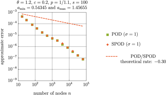
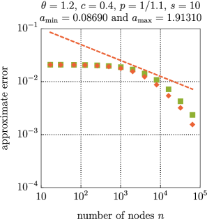
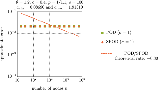
Figure 1: The kernel interpolation errors of the PDE problem (16)–(17) with $\theta=1.2$, $p=1/1.1$, $c\in\{0.2,0.4\}$, and $s\in\{10,100\}$. Results are displayed for kernel interpolants constructed using POD and SPOD weights. (Product weights (46) are not well-defined in this case.)

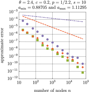
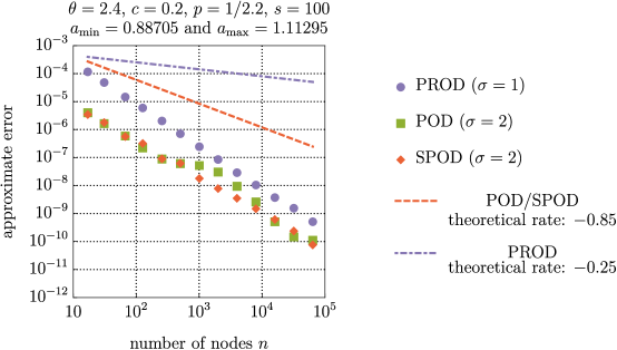
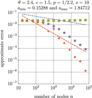
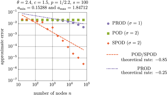
Figure 2: The kernel interpolation errors of the PDE problem (16)–(17) with $\theta=2.4$, $p=1/2.2$, $c\in\{0.2,1.5\}$, and $s\in\{10,100\}$. Results are displayed for kernel interpolants constructed using product (PROD), POD, and SPOD weights.

We approximate the dimensionally truncated finite element solution $u_{s,h}$ of the PDE (16)–(17) by constructing a kernel interpolant $u_{{s,h,n}}({\boldsymbol{x}},\boldsymbol{y}):=A^{\ast}_{n}(u_{s,h}({\boldsymbol{x}},\boldsymbol{y}))$, ${\boldsymbol{x}}\in D$ and $\boldsymbol{y}\in U_{s}$ using SPOD weights, POD weights, and product weights chosen according to Theorem 10, Theorem 11, and Theorem 12, respectively. The same weights appear in the formula for the kernel as well as the search criterion for finding good lattice generating vectors. The kernel interpolant is constructed over a lattice point set $\boldsymbol{t}_{k}:=\{k\boldsymbol{z}/n\}$, $k\in\{1,\ldots,n\}$, where the generating vector ${\boldsymbol{z}}\in\{1,\ldots,n-1\}^{s}$ has been obtained separately for each weight type using the fast CBC algorithm detailed in [4]. We assess the kernel interpolation error by computing

error $$\,=\,\sqrt{\int_{U_{s}}\int_{D}\big{(}u_{s,h}({\boldsymbol{x}},\boldsymbol{y})-u_{s,h,n}({\boldsymbol{x}},\boldsymbol{y})\big{)}^{2}\,{\rm d}{\boldsymbol{x}}\,{\rm d}\boldsymbol{y}}$$

$$\,\approx\,\sqrt{\frac{1}{Ln}\sum_{\ell=1}^{L}\sum_{k=1}^{n}\int_{D}\big{(}u_{s,h}\big{(}{\boldsymbol{x}},\boldsymbol{y}_{\ell}+\boldsymbol{t}_{k}\big{)}-u_{s,h,n}({\boldsymbol{x}},\boldsymbol{y}_{\ell}+\boldsymbol{t}_{k})\big{)}^{2}\,{\rm d}{\boldsymbol{x}}}\,,$$

where $\boldsymbol{y}_{\ell}$ for $\ell=1,\ldots,L$ is a sequence of Sobol^′ nodes in $[0,1]^{s}$, with $L=100$, and we recall that all our functions including $u_{s,h}({\boldsymbol{x}},\boldsymbol{y})$ and $u_{s,h,n}({\boldsymbol{x}},\boldsymbol{y})$ are $1$-periodic with respect to $\boldsymbol{y}$. The kernel interpolant in the formula above can be evaluated efficiently over the union of shifted lattices $\boldsymbol{y}_{\ell}+{\boldsymbol{t}}_{k}$, $\ell=1,\ldots,L$, $k=1,\ldots,n$, by making use of formula (49) in conjunction with the fast Fourier transform, requiring only the evaluation of the values $K({\boldsymbol{t}}_{k},\boldsymbol{y}_{\ell})$.

We compute the approximation error when $\theta\in\{1.2,2.4,3.6\}$, choosing $p\in\{\frac{1}{1.1},\frac{1}{2.2},\frac{1}{3.3}\}$, respectively, which are all $p$ values ensuring that (A3) is satisfied. We also use several values of the parameter $c\in\{0.2,0.4,1.5\}$ to control the difficulty of the problem. We set $\delta=0.1$ in the product weights (46). The numerical experiments have been carried out by using both $s=10$ and $s=100$ as the truncation dimensions. Selected results are displayed in Figures 1–3, where the corresponding values of $a_{\min}$ and $a_{\max}$ are listed to give insights to the difficulty of the problem in each case, as well as the parameter $\sigma$ which shows the “order” of the lattice rule. Note that as $s$ increases the problem does not change, but the computation becomes harder because the diffusion coefficient takes a wider range of values, with small values of $a({\boldsymbol{x}},\boldsymbol{y})$ being especially challenging.

The empirically obtained convergence rates appear to exceed the theoretically expected rates once the kernel interpolant enters the asymptotic regime of convergence. The convergence behavior of the kernel interpolant with SPOD weights is good across all experiments, except for the most difficult PDE problem of the lot corresponding to parameters $\theta=1.2$ and $c=0.4$, illustrated in the bottom row of Figure 1. On the other hand, the POD weights and, to a lesser extent, the product weights appear to be somewhat sensitive to the effective dimension of the PDE problem, either leading to a longer pre-asymptotic regime compared to SPOD weights (see “PROD” in the bottom row of Figure 2) or no apparent convergence (see “POD” in the bottom rows of Figures 2 and 3).

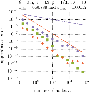
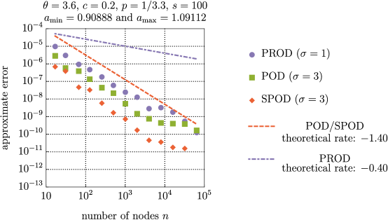
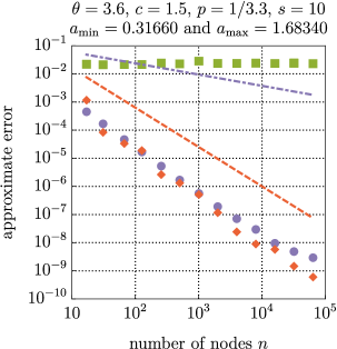
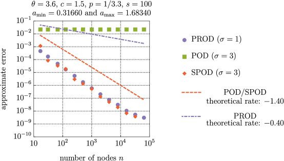
Figure 3: The kernel interpolation errors of the PDE problem (16)–(17) with $\theta=3.6$, $p=1/3.3$, $c\in\{0.2,1.5\}$, and $s\in\{10,100\}$. Results are displayed for kernel interpolants constructed using product (PROD), POD, and SPOD weights.

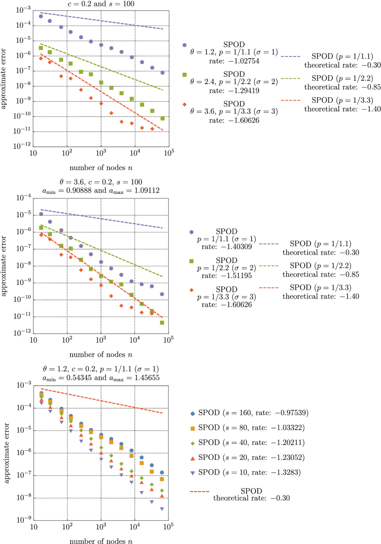
Figure 4: The kernel interpolation errors of the PDE problem (16)–(17) for kernel interpolants constructed using SPOD weights and varying parameters. Top: fixed $s=100$ and $c=0.2$ and different values of $\theta$. Middle: fixed $s=100$ and $\theta=3.6$, different values of $p$, and corresponding $\sigma=\sigma(p)$. Theoretical error-decay rate is $-\frac{1}{2p}+\frac{1}{4}=-0.3,-0.85,-1.4$ for $p=\frac{1}{1.1},\frac{1}{2.2},\frac{1}{3.3}$. Bottom: fixed $\theta=1.2$, $c=0.2$, $p=1/1.1$, and $\sigma=1$ with different values of $s\in\{10,20,40,80,160\}$.

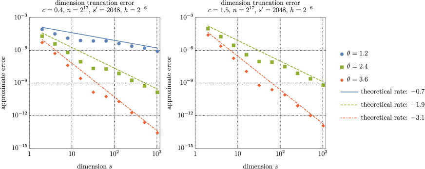
Figure 5: The dimension truncation errors of the PDE problem (16)–(17). Left: $c=0.4$ and $\theta\in\{1.2,2.4,3.6\}$. Right: $c=1.5$ and $\theta\in\{2.4,3.6\}$.

In the top graph of Figure 4 we compare the results in Figures 1–3 from SPOD weights with truncation dimension $s=100$ for the same damping parameter $c=0.2$ and different $\theta\in\{1.2,2.4,3.6\}$, listing the estimated convergence rate in each case. In the middle graph of Figure 4 we show the results of an additional experiment, namely, that for $s=100$ where we fix the decay rate $\theta=3.6$ of the stochastic fluctuations and solve the parametric PDE problem using different $\sigma\in\{1,2,3\}$ in the formula for SPOD weights, which correspond to $p\in\{\frac{1}{1.1},\frac{1}{2.2},\frac{1}{3.3}\}$, see Theorem 10. Finally, in the bottom graph of Figure 4, we return to the experimental setup illustrated in Figure 1 except this time we carry out the experiment using the truncation dimensions $s\in\{10,20,40,80,160\}$.

In all cases displayed in Figure 4, the observed error decays faster than the rate implied by Theorem 10. We also see that increasing $\sigma$ improves the error and mildly improves the rate of convergence. Moreover, we observe from the graph in the middle that the parameter $\theta$ that governs the decay of $\|\psi_{j}\|_{L_{\infty}(D)}$ is more important in determining the rate than the choice of $\sigma$. This observation suggests that the kernel interpolation with the rank-$1$ lattice points are robust in $\sigma$. Notice that $\sigma$ appears in the definition (40) of the SPOD weights; and that the weights are an input of the CBC construction, and are used to define the kernel $K(\cdot,\cdot)$. These observed error decay rates and the robustness are encouraging, but also suggest that the worst-case error estimates may be pessimistic in practical situations. The bottom graph in Figure 4 illustrates the effect that the truncation dimension has on the obtained convergence rates: we see that the observed convergence rate remains reasonable even when $s=160$.

Finally, we present numerical experiments that assess the dimension truncation error rate given in Theorem 6. We consider the same PDE and stochastic fluctuations $(\psi_{j})_{j\geq 1}$ which were stated at the beginning of this section. We choose the parameters $c=0.4$ with $\theta\in\{1.2,2.4,3.6\}$ and $c=1.5$ with $\theta\in\{2.4,3.6\}$. The PDE is discretized using piecewise linear finite element method with mesh size $h=2^{-6}$ and the integral over the computational domain $D$ is computed exactly for the finite element solutions. As the reference solution, we use the finite element solution with truncation dimension $s^{\prime}=2^{11}$. The dimension truncation error is then estimated by computing

$$\sqrt{\int_{U_{s^{\prime}}}\int_{D}(u_{s^{\prime},h}({\boldsymbol{x}},\boldsymbol{y})-u_{s,h}({\boldsymbol{x}},\boldsymbol{y}))^{2}\,{\rm d}{\boldsymbol{x}}\,{\rm d}\boldsymbol{y}}$$

for $s=2^{k}$, $k=2,\ldots,10$, where the value of the parametric integral is computed approximately by means of a rank-1 lattice rule based on the off-the-shelf generating vector lattice-39101-1024-1048576.3600 downloaded from https://web.maths.unsw.edu.au/~fkuo/lattice/ with $n=2^{17}$ nodes. The results are displayed in Figure 5. The theoretically expected rate, which is essentially $\mathcal{O}(s^{-\theta+1/2})$, is clearly observed in all cases.

7 Conclusions

In this paper we have developed an approximation scheme for periodic multivariate functions based on kernel approximation at lattice points, in the setting of weighted Hilbert spaces of dominating mixed smoothness. We have developed $L_{2}$ error estimates that are independent of dimension, for three classes of weights: product weights, POD (product and order dependent) weights and SPOD (smoothness driven product and order dependent) weights. Numerical experiments for 10 and 100 dimensions give results that (with the possible exception of POD weights) are generally satisfactory, and that exhibit better than predicted rates of convergence.

Nevertheless, there is room for future improvement. First, the error analysis is based on the principle that the $L_{2}$ error is bounded above by the worst case $L_{2}$ error multiplied by the norm of the function being approximated; yet it is known (see Section 3.1) that the worst-case error has a poor rate of convergence. It may be possible to obtain improved error rates by making better use of the special properties of the minimum norm interpolant in conjunction with the analytic parameter dependence of the PDE solution of (16)–(17).

References

[1]
G. Byrenheid, L. Kämmerer, T. Ullrich, and T. Volkmer.
Tight error bounds for rank- lattice sampling in spaces of hybrid mixed smoothness.
Numer. Math., 136:993–1034 (2017)
[2] P. G. Ciarlet. The Finite Element Method for Elliptic Problems. North-Holland Publishing Company (1978)
[3]
R. Cools, F. Y. Kuo, D. Nuyens, and I. H. Sloan.
Lattice algorithms for multivariate approximation in periodic spaces with general weight
parameters,
In: Celebrating 75 Years of Mathematics of Computation
(S. C. Brenner, I. Shparlinski, C.-W. Shu, and D. Szyld, eds.), Contemporary Mathematics, 754, AMS, 93–113 (2020)
[4]
R. Cools, F. Y. Kuo, D. Nuyens, and I. H. Sloan.
Fast component-by-component construction of lattice algorithms for multivariate approximation with POD and SPOD weights,
Math. Comp., 90: 787–812 (2021)
[5]
C. de Boor and R. E. Lynch.
On splines and their minimum properties.
J. Math. Mech., 15:953–969 (1966)
[6] R. N. Gantner.
Dimension truncation in QMC for affine-parametric operator equations.
In Monte Carlo and Quasi-Monte Carlo Methods 2016, pp. 249–264, Stanford, CA, August 14–19 (2018)
[7]
R. N. Gantner, L. Herrmann, and C. Schwab.
Quasi–Monte Carlo integration for affine-parametric, elliptic PDEs:
local supports and product weights.
SIAM J. Numer. Anal., 56(1):111–135 (2018)
[8]
M. Golomb and H. F. Weinberger.
Optimal approximation and error bounds.
In Numer. Approx. Proceedings a Symposium, Madison,
April 21–23, 1958, edited by R. E. Langer. Publication No. 1 of the
Mathematics Research Center, U.S. Army, the University of Wisconsin, pp.
117–190. The University of Wisconsin Press, Madison, Wis. (1959)
[9]
I. G. Graham, F. Y. Kuo, J. A. Nichols, R. Scheichl, C. Schwab, and I. H. Sloan.
Quasi-Monte Carlo finite element methods for elliptic PDEs with
lognormal random coefficients.
Numer. Math., 131(2):329–368 (2015)
[10]
M. Griebel and C. Rieger.
Reproducing kernel Hilbert spaces for parametric partial
differential equations.
SIAM/ASA J. Uncertain. Quantif., 5(1):111–137 (2017)
[11]
L. Herrmann and C. Schwab.
QMC integration for lognormal-parametric, elliptic PDEs: local
supports and product weights.
Numer. Math., 141(1):63–102 (2019)
[12]
V. Kaarnioja, F. Y. Kuo, and I. H. Sloan.
Uncertainty quantification using periodic random variables.
SIAM J. Numer. Anal.,58(2):1068–1091 (2020)
[13]
L. Kämmerer, D. Potts, and T. Volkmer.
Approximation of multivariate periodic functions by trigonometric polynomials based on rank- lattice sampling.
J. Complexity,31:543–576 (2015)
[14]
Y. Kazashi.
Quasi-Monte Carlo integration with product weights for elliptic
PDEs with log-normal coefficients.
IMA J. Numer. Anal., 39(3):1563–1593 (2019)
[15]
R. Kempf, H. Wendland, and C. Rieger.
Kernel-based reconstructions for parametric PDEs.
In Meshfree Methods
Partial Differ. Equations IX. IWMMPDE 2017, M. Griebel and M. Schweitzer, eds., pp. 53–71. Springer (2019)
[16]
F. Y. Kuo, G. Migliorati, F. Nobile, and D. Nuyens.
Function integration, reconstruction and approximation using rank-
lattices.
Math. Comp., 90:1861–1897 (2021)
[17]
F. Y. Kuo, C. Schwab, and I. H. Sloan.
Quasi-Monte Carlo finite element methods for a class of elliptic
partial differential equations with random coefficients.
SIAM J. Numer. Anal., 50(6):3351–3374 (2012)
[18] F. Y. Kuo, I. H. Sloan, and H. Woźniakowski.
Lattice rules for multivariate approximation in
the worst case setting. In
Monte Carlo and Quasi-Monte Carlo Methods 2004, H. Niederreiter and D. Talay, eds., pp. 289–330,
Springer (2006)
[19] F. Y. Kuo, I. H. Sloan, and H. Woźniakowski.
Lattice rule algorithms for multivariate approximation in the
average case setting.
J. Complexity, 24:283–323 (2008)
[20] C. A. Micchelli and T. J. Rivlin.
A survey of optimal recovery.
Optim. Estim. Approx. theory (Proc. Internat. Sympos.,
Freudenstadt, 1976), pp. 1–54 (1977)
[21] C. A. Micchelli and T. J. Rivlin.
Lectures on optimal recovery.
In: Turner P.R. (eds) Numerical Analysis Lancaster 1984. Lecture Notes in Mathematics, vol 1129. Springer (1985)
[22]
H. Rauhut and C. Schwab.
Compressive sensing Petrov-Galerkin approximation of
high-dimensional parametric operator equations.
Math. Comp., 86(304):661–700 (2016)
[23]
L. C. G. Rogers and D. Williams. Diffusions, Markov Processes, and Martingales. Vol. 1., 2nd edition, Cambridge University Press (2017)
[24]
I. H. Sloan and S. Joe.
Lattice Methods for Multiple Integration.
Oxford University Press (1994)
[25]
I. H. Sloan and H. Woźniakowski.
Tractability of multivariate integration for weighted Korobov classes.
J. Complexity, 17:697–721 (2001)
[26] H. Wendland.
Scattered Data Approximation.
Cambridge University Press (2005)
[27]
D. Xiu and G. E. Karniadakis.
The Wiener–Askey polynomial chaos for stochastic differential equations.
SIAM J. Sci. Comput.,
24:619–644 (2002)
[28] X. Y. Zeng, K. T. Leung, and F. J. Hickernell.
Error analysis of splines for periodic problems using lattice designs.
In
Monte Carlo and Quasi-Monte Carlo Methods 2004, H. Niederreiter and D. Talay, eds., pp. 501–514, Springer (2006)
[29] X. Y. Zeng, P. Kritzer, and F. J. Hickernell.
Spline methods using integration lattices and digital nets.
Constr. Approx., 30:529–555 (2009)