Quantitative Propagation of Chaos for SGD in Wide Neural Networks

Abstract

In this paper, we investigate the limiting behavior of a continuous-time counterpart of the Stochastic Gradient Descent (SGD) algorithm applied to two-layer overparameterized neural networks, as the number or neurons (i.e., the size of the hidden layer) $N\to+\infty$. Following a probabilistic approach, we show ‘propagation of chaos’ for the particle system defined by this continuous-time dynamics under different scenarios, indicating that the statistical interaction between the particles asymptotically vanishes. In particular, we establish quantitative convergence with respect to $N$ of any particle to a solution of a mean-field McKean-Vlasov equation in the metric space endowed with the Wasserstein distance. In comparison to previous works on the subject, we consider settings in which the sequence of stepsizes in SGD can potentially depend on the number of neurons and the iterations. We then identify two regimes under which different mean-field limits are obtained, one of them corresponding to an implicitly regularized version of the minimization problem at hand. We perform various experiments on real datasets to validate our theoretical results, assessing the existence of these two regimes on classification problems and illustrating our convergence results.

1 Introduction

Due to their ability to tackle very challenging problems, neural networks have been extremely popular and keystones in machine learning [1]. Thanks to their practical success, they have become the de facto tool in many application domains, such as image processing [2] and natural language processing [3]. However, the mathematical understanding of these models and their inherent inference mechanism still remains limited.

Among others, one suprising empirical observation about modern neural networks is that increasing the number of neurons in a network often leads to better classification testing and training errors [4], contradicting the classical statistical learning theory [5]. These experimental results suggest that neural network-based methods exhibit a limiting behavior when the number of neurons is large, i.e., when the neural network is overparameterized.

In this paper, we contribute to the recent literature on the theoretical analysis of this phenomenon. To this end, we consider a simple two-layer (i.e., one hidden layer) neural network that is parametrized by $N$ weights $w^{1:N}=\{w^{k,N}\}_{k=1}^{N}$ and trained to minimize the structural risk $\mathscr{R}^{N}$ by Stochastic Gradient Descent (SGD) using independent and identically distributed (i.i.d.) samples $(X_{i},Y_{i})_{i\in\mathbb{N}^{\star}}$. Even in such a simplified setting, the landscape of $\mathscr{R}^{N}$ is in many cases arduous to be explored, since $\mathscr{R}^{N}$ is non-convex and might exhibit many local minima and saddle points [6, 7]; hence making the minimization of $\mathscr{R}^{N}$ challenging. However, for large $N$, the analysis of the landscape of $\mathscr{R}^{N}$ turns out to be much simpler in some situations. For instance [8] has shown that local minima are global minima when the activation function is quadratic as soon as $N$ is larger than twice the size of the original dataset. More generally, relying on approximation or random matrix theory, several works (e.g.,[9, 10, 11, 12, 13, 14, 15, 16, 17, 18, 19]) establish favorable properties for the landscape of $\mathscr{R}^{N}$ as $N\to+\infty$, such as absence of saddle points, poor local minima or connected optima. In addition, minimization by SGD in this setting has also proved to be efficient for some models [20, 21].

In this paper we follow an increasingly popular line of research to analyze the behavior of gradient descent-type algorithms (stochastic or deterministic) used for overparameterized models. This approach consists in establishing a ‘continuous mean-field limit’ for these algorithms as $N\to+\infty$, and has been successively applied in [22, 23, 24, 25, 26, 27, 28, 29]. Based on this result, the qualitative long-time behavior of SGD applied to overparameterized neural networks can be deduced: these studies all identify an evolution equation on the limiting probability measure which corresponds to a mean-field ordinary differential equation (ODE), i.e., if the initialization is deterministic, then each hidden unit of the network independently evolves along the flow of a specific ODE. This implies that, even though the update step is intrinsically stochastic in SGD, the noise completely vanishes in the limit $N\to+\infty$. In this context, two main strategies have been followed to prove convergence of SGD to this mean-field dynamics. The first one is based on gradient flows in Wasserstein spaces [30, 31, 32] and the second one is the ‘propagation of chaos’ phenomenon [33, 34, 35], indicating that the statistical interaction between the individual entries of the network asymptotically vanishes. Both approaches are in fact deeply connected, which stems from the duality between probability and partial differential equation theories [36]. We follow in this paper the second approach and establish that propagation of chaos holds for a continuous counterpart of SGD to a solution of a McKean-Vlasov type diffusion [37] as $N\to+\infty$.

The fact that no noise appears in the mean-field limit of SGD obtained in previous work can seem surprising. Aiming to demystify this matter, we study in this paper the case where the stepsize in SGD can depend on the number of neurons. Our main contribution is to identify two mean-field regimes: The first one is the same as the deterministic mean-field limit obtained in the described literature. The second one is a McKean-Vlasov diffusion for which the covariance matrix is non-zero and depends on the properties of the data distribution. To the best of our knowledge, this limiting diffusion has not been reported in the literature and brings interesting insights on the behavior of neural networks in overparameterized settings. Our results suggest that taking large stepsizes in the stochastic optimization procedure corresponds to an implicit regularization of the original problem, which can potentially ease the minimization of the structural risk. In addition, in contrast to previous studies, we establish strong quantitative propagation of chaos and we identify the convergence rate of each neuron to its mean-field limit with respect to $N$. Finally we numerically illustrate the existence of these two regimes and the propagation of chaos phenomenon we derive on several classical classification examples on MNIST and CIFAR-10 datasets. In these experiments, the stochastic regime empirically exhibits slightly better generalization properties compared to the deterministic case identified in [22, 23, 28].

2 Overparametrized Neural Networks

Consider some feature and label spaces denoted by $\mathsf{X}$ and $\mathsf{Y}$ endowed with $\sigma$-fields $\mathcal{X}$ and $\mathcal{Y}$ respectively. In this paper, we consider a one hidden layer neural network, whose purpose is to classify data from $\mathsf{X}$ with labels in $\mathsf{Y}$. We suppose that the network has $N\in\mathbb{N}^{\star}$ neurons in the hidden layer whose weights are denoted by $w^{1:N}=\{w^{k,N}\}_{k=1}^{N}\in{(\mathbb{R}^{p})}^{N}$. We model the non-linearity by a function $F:\mathbb{R}^{p}\times\mathsf{X}\to\mathbb{R}$, and consider a loss function $\ell:\mathbb{R}\times\mathsf{Y}\to\mathbb{R}_{+}$ and a penalty function $V:\ \mathbb{R}^{p}\to\mathbb{R}$. Then, the learning problem corresponding to this space of hypothesis consists in minimizing the structural risk

$$\textstyle{\mathscr{R}^{N}(w^{1:N})=\int_{\mathsf{X}\times\mathsf{Y}}\ell\left(\dfrac{1}{N}\sum_{k=1}^{N}F(w^{k,N},x),y\right)\mathrm{d}\pi(x,y)+\dfrac{1}{N}\sum_{k=1}^{N}V(w^{k,N})\;,}$$ (1)

where $\pi$ is the data distribution on $\mathsf{X}\times\mathsf{Y}$. Note that, in this particular setting, the weights of the second layer are fixed to $(1/N)$. This setting is referred to as “fixed coefficients” in [25, Theorem 1] and is less realistic than the fully-trainable setting. Nevertheless, we believe that this shortcoming can be circumvented upon replacing $F(w^{k,N},\cdot)$ by $F(u^{k,N},\cdot)v^{k,N}$ in (1), where $u^{1:N}$ and $v^{1:N}$ are the weights of the hidden and the second layer respectively. However, this raises new theoretical challenges which are left for future work.

Throughout this paper, we consider the following assumptions.

A 1.

There exist measurable functions $\Phi:\mathsf{X}\to\left[1,+\infty\right)$ and $\Psi:\mathsf{Y}\to\left[1,+\infty\right)$ such that the following conditions hold.

1. $\ell:\ \mathbb{R}\times\mathbb{R}\to\mathbb{R}_{+}$ is such that for any $y\in\mathsf{Y}$, $(\tilde{\mathrm{y}}\mapsto\ell(\tilde{\mathrm{y}},y))$ is three-times differentiable and for any $\mathrm{y}\in\mathbb{R}$ and $y\in\mathsf{Y}$ we have

   $$\left|\partial_{1}\ell(0,y)\right|\leq\Psi(y)\;,\qquad\left|\partial_{1}^{2}\ell(\mathrm{y},y)\right|+\left|\partial_{1}^{3}\ell(\mathrm{y},y)\right|\leq\Psi(y)\;,$$ (2)

   where for any $i\in\{1,2,3\}$, $\partial_{1}^{i}\ell(\mathrm{y},y)$ is the $i$-th derivative of $(\tilde{\mathrm{y}}\mapsto\ell(\tilde{\mathrm{y}},y))$ at $\mathrm{y}$.

2. $F:\ \mathbb{R}^{p}\times\mathsf{X}\to\mathbb{R}$ is such that for any $x\in\mathsf{X}$, $(\tilde{w}\mapsto F(\tilde{w},x))$ is three-times differentiable and for any $w\in\mathbb{R}^{p}$ and $x\in\mathsf{X}$

   $$\left\|F(w,x)\right\|+\left\|\mathrm{D}_{w}^{1}F(w,x)\right\|+\left\|\mathrm{D}_{w}^{2}F(w,x)\right\|+\left\|\mathrm{D}_{w}^{3}F(w,x)\right\|\leq\Phi(x)\;,$$ (3)

   where for any $i\in\{1,2,3\}$, $\mathrm{D}_{w}^{i}F(w,x)$ is the $i$-th differential of $(\tilde{w}\mapsto F(\tilde{w},x))$ at $w$.

3. $V\in\mathrm{C}^{3}(\mathbb{R}^{p},\mathbb{R})$ satisfies $\sup_{w\in\mathbb{R}^{p}}\{\|\mathrm{D}^{2}V(w)\|+\|\mathrm{D}^{3}V(w)\|\}<+\infty$.

4. The data distribution $\pi$ satisfies $\int_{\mathsf{X}\times\mathsf{Y}}\{\Phi^{10}(x)+\Psi^{4}(y)\}\mathrm{d}\pi(x,y)<\infty\;.$

Note that 1-(d) is immediately satisfied in the case where $\pi$ is compactly supported, $\mathsf{X}$ and $\mathsf{Y}$ are subsets of $\mathbb{R}^{d}$ and $\mathbb{R}$ respectively and $\Psi$ and $\Phi$ are bounded on the support of $\pi$. For any $N\in\mathbb{N}^{\star}$, under 1, by the Lebesgue dominated convergence theorem, $\mathscr{R}^{N}$ given by (1) is well-defined, continuously differentiable with gradient given for any $w^{1:N}\in(\mathbb{R}^{p})^{N}$ by

$$\nabla\mathscr{R}^{N}(w^{1:N}) =\int_{\mathsf{X}\times\mathsf{Y}}\nabla_{w}\hat{\mathscr{R}}^{N}(w^{1:N},x,y)\mathrm{d}\pi(x,y)\;,$$ (4)

$$\hat{\mathscr{R}}^{N}(w^{1:N},x,y) =\textstyle{\ell\left(\frac{1}{N}\sum_{k=1}^{N}F(w^{k,N},x),y\right)+\frac{1}{N}\sum_{k=1}^{N}V(w^{k,N})}\;,$$

$$N\nabla_{w}\hat{\mathscr{R}}^{N}(w^{1:N},x,y) =\textstyle{\partial_{1}\ell\left(\frac{1}{N}\sum_{k=1}^{N}F(w^{k,N},x),y\right)\nabla_{w}F^{1:N}(w^{1:N},x)}+\nabla V^{1:N}(w^{1:N})\;,$$

setting $\nabla_{w}F^{1:N}(w^{1:N},x)=\{\nabla_{w}F(w^{k,N},x)\}_{k=1}^{N}$, and $\nabla V^{1:N}(w^{1:N})=\{\nabla V(w^{k,N})\}_{k=1}^{N}$.

Let $(W_{0}^{k})_{k\in\mathbb{N}^{\star}}$ be i.i.d. $p$ dimensional random variables with distribution $\mu_{0}$. Consider the sequence $(W_{n}^{1:N})_{n\in\mathbb{N}}$ associated with SGD, starting from $W_{0}^{1:N}$ and defined by the following recursion: for any $n\in\mathbb{N}$ denoting the iteration index

$$W^{1:N}_{n+1}=W^{1:N}_{n}-\gamma N^{\beta}(n+\gamma_{\alpha,\beta}(N)^{-1})^{-\alpha}\nabla\hat{\mathscr{R}}^{N}(W^{1:N}_{n},X_{n},Y_{n})\;,$$ (5)

where $(X_{n},Y_{n})_{n\in\mathbb{N}}$ is a sequence of i.i.d. input/label samples distributed according to $\pi$, and $(\gamma N^{\beta}(n+\gamma_{\alpha,\beta}(N)^{-1})^{-\alpha})_{n\in\mathbb{N}}$ as a whole denotes a sequence of stepsizes: here, $\beta\in\left[0,1\right]$, $\alpha\in\left[0,1\right)$, and $\gamma_{\alpha,\beta}(N)=\gamma^{1/(1-\alpha)}N^{(\beta-1)/(1-\alpha)}$. Note that in the constant stepsize setting $\alpha=0$, the recursion (5) consists in using $\gamma N^{\beta}$ as a stepsize In addition, it also encompasses the case of decreasing stepsizes (as soon as $\alpha>0$). The term $\gamma_{\alpha,\beta}(N)^{-1}$ in (5) is a scaling parameter which appears naturally in the corresponding continuous-time dynamics, see (9) below. We stress that contrary to previous approaches such as [28, 23, 22], the stepsize appearing in (5) depends on the number of neurons $N$. Our main contribution is to establish that different mean-field limiting behaviors of a continuous counterpart of SGD arise depending on $\beta$.

We will show that the quantity $\gamma_{\alpha,\beta}(N)$ plays the role of a discretization stepsize in the McKean-Vlasov approximation of SGD. The case where $\alpha=0$ and $\beta=0$, i.e., the setting considered by [28, 23, 22], corresponds to choosing the stepsize as $\gamma/N$, which decreases with increasing $N$. In the new setting $\alpha=0$, $\beta=1$, this corresponds to take a fixed stepsize $\gamma$. This observation further motivates the scaling and the parameter we introduced in (5).

Before stating our result, we present and give an informal derivation of the continuous particle system dynamics we consider to model (5). We first show that (5) can be rewritten as a recursion corresponding to the discretization of a continuous particle system, i.e., a stochastic differential equation (SDE) with coefficients depending on the empirical measure of the particles. Let us denote by $\mathscr{P}(\mathsf{E})$ the set of probability measures on a measurable space $(\mathsf{E},\mathcal{E})$. Remark that for each particle dynamics $(W_{n}^{k,N})_{n\in\mathbb{N}}$ the SGD update (5) is a function of the current position and the empirical measure of the weights. To show this, define the mean-field $h:\mathbb{R}^{p}\times\mathscr{P}(\mathbb{R}^{d})\to\mathbb{R}^{p}$ and the noise field $\xi:\mathbb{R}^{p}\times\mathscr{P}(\mathbb{R}^{d})\times\mathsf{X}\times\mathsf{Y}\to\mathbb{R}^{p}$, for any $\mu\in\mathscr{P}(\mathbb{R}^{p})$, $w\in\mathbb{R}^{p}$, $(x,y)\in\mathsf{X}\times\mathsf{Y}$ by

$$h(w,\mu)=-\int_{\mathsf{X}\times\mathsf{Y}}\partial_{1}\ell\left(\mu[F(\cdot,x)],y\right)\nabla_{w}F(w,x)\,\mathrm{d}\pi(x,y)-\nabla V(w)\;,$$ (6)

$$\xi(w,\mu,x,y)=-h(w,\mu)-\partial_{1}\ell(\mu[F(\cdot,x)],y)\nabla_{w}F(w,x)-\nabla V(w)\;.$$ (7)

Note that with this notation, $h(w^{k,N},\nu_{n}^{N})=-N\partial_{w^{k,N}}\mathscr{R}^{N}(w^{1:N})$ and $\xi(w^{k,N},\nu_{n}^{N},X_{n},Y_{n})=N\{-\partial_{w^{k,N}}\hat{\mathscr{R}}^{N}(w^{1:N},X_{n},Y_{n})+\partial_{w^{k,N}}\mathscr{R}^{N}(w^{1:N})\}$, for any $N\in\mathbb{N}$, $k\in\{1,\dots,N\}$ and $n\in\mathbb{N}$, where $\nu^{N}$ is the empirical measure of the discrete particle system corresponding to SGD defined by $\nu_{n}^{N}=N^{-1}\sum_{k=1}^{N}\updelta_{W^{k,N}_{n}}$. Then, the recursion (5) can be rewritten as follows:

$$W^{k,N}_{n+1}=W^{k,N}_{n}+\gamma N^{\beta-1}(n+\gamma_{\alpha,\beta}(N)^{-1})^{-\alpha}\left\{h(W^{k,N}_{n},\nu_{n}^{N})+\xi(W^{k,N}_{n},\nu_{n}^{N},X_{n},Y_{n})\right\}\;.$$ (8)

We now present the continuous model associated with this discrete process. For large $N$ or small $\gamma$ these two processes can be arbitrarily close. For $N\in\mathbb{N}^{\star}$, consider the particle system diffusion $(\mathbf{W}^{1:N}_{t})_{t\geq 0}=(\{\mathbf{W}^{k,N}_{t}\}_{k=1}^{N})_{t\geq 0}$ starting from $\mathbf{W}^{1:N}_{0}=W_{0}^{1:N}$ defined for any $k\in\{1,\dots,N\}$ by

$$\mathrm{d}\mathbf{W}^{k,N}_{t}=(t+1)^{-\alpha}\left\{h(\mathbf{W}^{k,N}_{t},\bm{\nu}^{N}_{t})\mathrm{d}t+\gamma_{\alpha,\beta}(N)^{1/2}\Sigma^{1/2}(\mathbf{W}^{k,N}_{t},\bm{\nu}^{N}_{t})\mathrm{d}\mathbf{B}^{k}_{t}\right\}\;,$$ (9)

where $\{(\mathbf{B}_{t}^{k})_{t\geq 0}\,:\;k\in\mathbb{N}^{\star}\}$ is a family of independent $p$-dimensional Brownian motions and $\bm{\nu}^{N}_{t}$ is the empirical probability distribution of the particles defined for any $t\geq 0$ by $\bm{\nu}^{N}_{t}=N^{-1}\sum_{k=1}^{N}\updelta_{\mathbf{W}^{k,N}_{t}}$. In addition in (9), $\Sigma$ is the $p\times p$ matrix given by

$$\textstyle{\Sigma(w,\mu)=\int_{\mathsf{X}\times\mathsf{Y}}\xi(w,\mu,x,y)\xi(w,\mu,x,y)^{\top}\mathrm{d}\pi(x,y)\;,}\qquad\text{ for any $w\in\mathbb{R}^{p}$ and $\mu\in\mathscr{P}(\mathbb{R}^{p})$}\;,$$ (10)

which is well-defined under 1. In the supplementary material we show that under 1, (9) admits a unique strong solution. We now give an informal discussion to justify why (9) can be seen as the continuous-time counterpart of (8). For any $N\in\mathbb{N}^{\star}$, define $(\tilde{\mathbf{W}}^{1:N}_{t})_{t\geq 0}$ for any $t\geq 0$ by $\tilde{\mathbf{W}}^{1:N}_{t}=W_{n_{t}}^{1:N}$ with $n_{t}=\left\lfloor t/\gamma_{\alpha,\beta}(N)\right\rfloor$ and denote $\tilde{\bm{\nu}}^{N}_{t}$ the empirical measure associated with $\tilde{\mathbf{W}}^{1:N}_{t}$. In this case, by defining the interval $I_{n,\alpha,\beta}^{N}=\left[n\gamma_{\alpha,\beta}(N),(n+1)\gamma_{\alpha,\beta}(N)\right]$ and using (8) and $\gamma_{\alpha,\beta}(N)^{1-\alpha}=\gamma N^{\beta-1}$, we obtain the following approximation for any $n\in\mathbb{N}$

$$\tilde{\mathbf{W}}^{k,N}_{(n+1)\gamma_{\alpha,\beta}(N)}-\tilde{\mathbf{W}}^{k,N}_{n\gamma_{\alpha,\beta}(N)}$$ (11)

$$=\gamma N^{\beta-1}(n+\gamma_{\alpha,\beta}(N)^{-1})^{-\alpha}\left\{h(\tilde{\mathbf{W}}^{k,N}_{n\gamma_{\alpha,\beta}(N)},\nu_{n}^{N})+\xi(\tilde{\mathbf{W}}^{k,N}_{n\gamma_{\alpha,\beta}(N)},\nu_{n}^{N},X_{n},Y_{n})\right\}$$ (12)

$$\approx\gamma_{\alpha,\beta}(N)(n\gamma_{\alpha,\beta}(N)+1)^{-\alpha}\left\{h(\tilde{\mathbf{W}}^{k,N}_{n\gamma_{\alpha,\beta}(N)},\tilde{\bm{\nu}}^{N}_{n\gamma_{\alpha,\beta}(N)})+\Sigma^{1/2}(\tilde{\mathbf{W}}^{k,N}_{n\gamma_{\alpha,\beta}(N)},\tilde{\bm{\nu}}^{N}_{n\gamma_{\alpha,\beta}(N)})G\right\}$$ (13)

$$\approx\underbrace{\int_{I_{n,\alpha,\beta}^{N}}(s+1)^{-\alpha}h(\tilde{\mathbf{W}}^{k,N}_{s},\tilde{\bm{\nu}}^{N}_{s})\mathrm{d}s}_{(A)}+\underbrace{\int_{I_{n,\alpha,\beta}^{N}}\gamma^{1/2}_{\alpha,\beta}(N)(s+1)^{-\alpha}\Sigma^{1/2}(\tilde{\mathbf{W}}^{k,N}_{s},\tilde{\bm{\nu}}^{N}_{s})\mathrm{d}\mathbf{B}_{s}^{k}}_{(B)}\;,$$ (14)

where $G$ is a $p$-dimensional Gaussian random variable with zero mean and identity covariance matrix. Note that the second line corresponds to (8) and the last to (9). To obtain such proxy, we first remark that for any $w\in\mathbb{R}^{p}$ and $\mu\in\mathscr{P}(\mathbb{R}^{p})$, $\xi(w,\mu,X_{n},Y_{n})$ has zero mean and covariance matrix $\Sigma(w,\mu)$ and assume that the noise term is roughly Gaussian. Second, we use that the covariance of $(B)$ in (14) is equal to $\int_{I_{n,\alpha,\beta}^{N}}\gamma_{\alpha,\beta}(N)(s+1)^{-2\alpha}\Sigma(\tilde{\mathbf{W}}^{k,N}_{s},\tilde{\bm{\nu}}^{N}_{s})\mathrm{d}s$. To obtain the last line, we use some first-order Taylor expansion of this term and $(A)$ as $\gamma_{\alpha,\beta}(N)\to 0$. Then, (14) corresponds to (9) on $I_{n,\alpha,\beta}^{N}$. As a result, (9) is the continuous counterpart to (8) and $n$ iterations in (8) correspond to the horizon time $n\gamma_{\alpha,\beta}(N)$ in (9). In the next section, we show that a strong quantitative propagation of chaos holds for (9) i.e., we show that for $N\to+\infty$ the particles become indenpendent and have the same distribution associated with a McKean-Vlasov diffusion. The extension of these results to discrete SGD (8) and the rigorous derivation of (14) can be established using strong functional approximations following [38, Proposition 1]. Due to space constraints, we leave it as future work.

Finally, note that until now we only considered the case where the batch size in SGD is equal to one. For a batch size $M\in\mathbb{N}^{\star}$, this limitation can be lifted replacing $\pi$ and $\hat{\mathscr{R}}^{N}$ in (5) by $\pi^{\otimes M}$ and

$$\textstyle{\hat{\mathscr{R}}^{N,M}(w^{1:N},x,y)=\dfrac{1}{M}\sum_{i=1}^{M}\ell\left(\dfrac{1}{N}\sum_{k=1}^{N}F(w^{k,N},x_{i}),y_{i}\right)\;,}$$ (15)

defined for any $w^{1:N}\in(\mathbb{R}^{p})^{N}$, $x=(x_{i})_{i\in\{1,\dots,M\}}\in\mathsf{X}^{M}$ and $y=(y_{i})_{i\in\{1,\dots,M\}}\in\mathsf{Y}^{M}$. In this case, we obtain that the continuous-time counterpart of (8) is given by (9) upon replacing $\Sigma^{1/2}$ by $\Sigma^{1/2}/M^{1/2}$. This leads to the particle system diffusion $(\mathbf{W}^{1:N}_{t})_{t\geq 0}=(\{\mathbf{W}^{k,N}_{t}\}_{k=1}^{N})_{t\geq 0}$ starting from $\mathbf{W}^{1:N}_{0}$ defined for any $k\in\{1,\dots,N\}$ by

$$\mathrm{d}\mathbf{W}^{k,N}_{t}=(t+1)^{-\alpha}\left\{h(\mathbf{W}^{k,N}_{t},\bm{\nu}^{N}_{t})\mathrm{d}t+(\gamma_{\alpha,\beta}(N)/M)^{1/2}\Sigma^{1/2}(\mathbf{W}^{k,N}_{t},\bm{\nu}^{N}_{t})\mathrm{d}\mathbf{B}^{k}_{t}\right\}\;.$$ (16)

In the supplement Section 7, we also present the case of a modified Stochastic Gradient Langevin Dynamics (mSGLD) algorithm [39] which was considered in [23] in the specific case $\beta=0$. We extend our propagation of chaos results to this setting.

3 Mean-Field Approximation and Propagation of Chaos

In this section we identify the mean-field limit of the diffusion (16). More precisely, we show that there exist two regimes depending on how the stepsize scale with the number of hidden units.

Our results are based on the propagation of chaos theory [33, 35, 34] and extend the recent works of [27, 28, 40, 22, 25, 23]. In what follows, we denote $\mathscr{P}_{2}(\mathbb{R}^{p})=\{\mu\in\mathscr{P}(\mathbb{R}^{p})\,:\,\int_{\mathbb{R}^{p}}\left\|\tilde{w}\right\|^{2}\mathrm{d}\mu(\tilde{w})<+\infty\}$ and $\mathrm{C}(\mathbb{R}_{+},\mathbb{R}^{p})$ the set of continuous functions from $\mathbb{R}_{+}$ to $\mathbb{R}^{p}$. We also consider the usual metric $\mathrm{m}$ on $\mathrm{C}(\mathbb{R}_{+},\mathbb{R}^{p})$ defined for any $u_{1},u_{2}\in\mathrm{C}(\mathbb{R}_{+},\mathbb{R}^{p})$ by $\mathrm{m}(u_{1},u_{2})=\sum_{n\in\mathbb{N}^{\star}}2^{-n}\left\|u_{1}-u_{2}\right\|_{\infty,n}/\{1+\left\|u_{1}-u_{2}\right\|_{\infty,n}\}$, where $\left\|u_{1}-u_{2}\right\|_{\infty,n}=\sup_{t\in\left[0,n\right]}\|u_{1}(t)-u_{2}(t)\|$. It is well-known that $(\mathscr{C},\mathrm{m})=(\mathrm{C}(\mathbb{R}_{+},\mathbb{R}^{p}),\mathrm{m})$ is a complete separable space. For any metric space $(\mathsf{F},\mathrm{m}_{\mathsf{F}})$, with Borel $\sigma$-field $\mathcal{B}(\mathsf{F})$, we define the extended Wasserstein distance of order $2$, denoted $\mathpzc{W}_{2}:\ \mathscr{P}(\mathsf{F})\times\mathscr{P}(\mathsf{F})\to\left[0,+\infty\right]$ for any $\mu_{1},\mu_{2}\in\mathscr{P}(\mathsf{F})$ by $\mathpzc{W}_{2}^{2}(\mu_{1},\mu_{2})=\inf_{\Lambda\in\Gamma(\mu_{1},\mu_{2})}\int_{\mathsf{F}\times\mathsf{F}}\mathrm{m}_{\mathsf{F}}^{2}(v_{1},v_{2})\mathrm{d}\Lambda(v_{1},v_{2})$, where $\Gamma(\mu_{1},\mu_{2})$ is the set of transference plans between $\mu_{1}$ and $\mu_{2}$, i.e., $\Lambda\in\Gamma(\mu_{1},\mu_{2})$ if for any $\mathsf{A}\in\mathcal{B}(\mathsf{F})$, $\Lambda(\mathsf{A}\times\mathsf{F})=\mu_{1}(\mathsf{A})$ and $\Lambda(\mathsf{F}\times\mathsf{A})=\mu_{2}(\mathsf{A})$.

We start by stating our results in the case where $\beta\in\left[0,1\right)$ for which a deterministic mean-field limit is obtained. Consider the mean-field ODE starting from a random variable $\mathbf{W}_{0}^{\star}$ given by

$$\mathrm{d}\mathbf{W}_{t}^{\star}=(t+1)^{-\alpha}h(\mathbf{W}_{t}^{\star},\bm{\lambda}_{t}^{\star})\mathrm{d}t\;,\qquad\text{with $\bm{\lambda}^{\star}_{t}$ the distribution of $\mathbf{W}_{t}^{\star}$}\;.$$ (17)

We show in the supplement that this ODE admits a solution on $\mathbb{R}_{+}$. This mean-field equation (17) is deterministic conditionally to its initialization.

Theorem 1.

Assume 1. Let $(\mathbf{W}_{0}^{k})_{k\in\mathbb{N}}$ be a sequence of i.i.d. $\mathbb{R}^{p}$-valued random variables with distribution $\mu_{0}\in\mathscr{P}_{2}(\mathbb{R}^{p})$ and set for any $N\in\mathbb{N}^{\star}$, $\mathbf{W}_{0}^{1:N}=\{\mathbf{W}_{0}^{k}\}_{k=1}^{N}$. Then, for any $m\in\mathbb{N}^{\star}$ and $T\geq 0$, there exists $C_{m,T}\geq 0$ such that for any $\alpha\in\left[0,1\right)$, $\beta\in\left[0,1\right)$, $M\in\mathbb{N}^{\star}$ and $N\in\mathbb{N}^{\star}$ with $N\geq m$

$$\textstyle{\mathbb{E}\left[\sup_{t\in\left[0,T\right]}\|\mathbf{W}_{t}^{1:m,N}-\mathbf{W}_{t}^{1:m,\star}\|^{2}\right]\leq C_{m,T}\left\{N^{-(1-\beta)/(1-\alpha)}M^{-1}+N^{-1}\right\}\;,}$$ (18)

with $(\mathbf{W}_{t}^{1:m,N},\mathbf{W}_{t}^{1:m,\star})=\{(\mathbf{W}_{t}^{k,N},\mathbf{W}_{t}^{k,\star})\}_{k=1}^{m}$, $(\mathbf{W}_{t}^{1:N})$ the solution of (16) starting from $\mathbf{W}_{0}^{1:N}$, and for any $k\in\mathbb{N}^{\star}$, $\mathbf{W}_{t}^{k,\star}$ the solution of (17) starting from $\mathbf{W}_{0}^{k}$.

In Theorem 1, $m$ is a fixed number of particles. Note that $\{(\mathbf{W}_{t}^{k,\star})_{t\geq 0}\,:\;k\in\mathbb{N}^{\star}\}$ is i.i.d. with distribution $\bm{\lambda}^{\star}$ which is the pushfoward measure of $\mu_{0}$ by the function $(w_{0}\mapsto(w_{t})_{t\geq 0})$ which from an initial point $w_{0}$ gives $(w_{t})_{t\geq 0}\in\mathscr{C}$ the solution of (17) on $\mathbb{R}_{+}$. Theorem 1 shows that the dynamics of the particles become deterministic and independent when $N\to+\infty$. The proofs of Theorem 1 and the following result, Theorem 2, are postponed to Section 9.4.

We now consider the case $\beta=1$ and derive a similar quantitative theorem as Theorem 1 but with a different dynamics than (17). Consider the mean-field SDE starting from variable $\mathbf{W}_{0}^{\star}$ given by

$$\mathrm{d}\mathbf{W}_{t}^{\star}=(t+1)^{-\alpha}\left\{h(\mathbf{W}_{t}^{\star},\bm{\lambda}_{t}^{\star})\mathrm{d}t+(\gamma^{1/(1-\alpha)}\Sigma(\mathbf{W}_{t}^{\star},\bm{\lambda}_{t}^{\star})/M)^{1/2}\mathrm{d}\mathbf{B}_{t}\right\}\;,$$ (19)

where $\bm{\lambda}^{\star}_{t}$ is the distribution of $\mathbf{W}_{t}^{\star}$ and $(\mathbf{B}_{t})_{t\geq 0}$ is a $p$ dimensional Brownian motion. Note that taking the limit $\gamma\to 0$ or $M\to+\infty$ in (19) we recover (17). We show in the supplement that this SDE admits a solution on $\mathbb{R}_{+}$. The following theorem is similar to Theorem 1 in the case $\beta=1$.

Theorem 2.

Let $\beta=1$. Assume 1. Let $(\mathbf{W}_{0}^{k})_{k\in\mathbb{N}}$ be a sequence of $\mathbb{R}^{p}$-valued random variables with distribution $\mu_{0}\in\mathscr{P}_{2}(\mathbb{R}^{p})$ and assume that for any $N\in\mathbb{N}^{\star}$, $\mathbf{W}_{0}^{1:N}=\{\mathbf{W}_{0}^{k}\}_{k=1}^{N}$. Then, for any $m\in\mathbb{N}^{\star}$ and $T\geq 0$, there exists $C_{m,T}\geq 0$ such that for any $\alpha\in\left[0,1\right)$, $M\in\mathbb{N}^{\star}$ and $N\in\mathbb{N}^{\star}$ with $N\geq m$

$$\textstyle{\mathbb{E}\left[\sup_{t\in\left[0,T\right]}\|\mathbf{W}_{t}^{1:m,N}-\mathbf{W}_{t}^{1:m,\star}\|^{2}\right]\leq C_{m,T}N^{-1}\;,}$$ (20)

with $(\mathbf{W}_{t}^{1:m,N},\mathbf{W}_{t}^{1:m,\star})=\{(\mathbf{W}_{t}^{k,N},\mathbf{W}_{t}^{k,\star})\}_{k=1}^{m}$, $(\mathbf{W}_{t}^{1:N})$ the solution of (16) starting from $\mathbf{W}_{0}^{1:N}$, and for any $k\in\mathbb{N}^{\star}$, $\mathbf{W}_{t}^{k,\star}$ the solution of (19) starting from $\mathbf{W}_{0}^{k}$ and Brownian motion $(\mathbf{B}^{k}_{t})_{t\geq 0}$.

The main difference between (17) and (19) is that now this mean-field limit is now longer deterministic up to its initialization but is a SDE driven by a Brownian motion. The stochastic nature of SGD is preserved in this second regime. (17) corresponds to some implicit regularization of (19). In the case where for any $w\in\mathbb{R}^{p}$ and $\mu\in\mathscr{P}(\mathbb{R}^{p})$, $\Sigma(w,\mu)=\upsigma^{2}\operatorname{Id}$ with $\upsigma>0$, it can shown that $(\bm{\lambda}_{t}^{\star})_{t\geq 0}$ is a gradient flow for an entropic-regularized functional. This relation between our approach and the gradient flow perspective is investigated in the supplement Section 11.

Denote for any $N\in\mathbb{N}^{\star}$ and $m\in\{1,\dots,N\}$, $\bm{\lambda}^{1:m,N}$ the distribution on $\mathscr{C}$ of $\{(\mathbf{W}_{t}^{k,N})_{t\geq 0}\}_{k=1}^{m}$. Recall that $\{\mathbf{W}_{0}^{k,N}\}_{k=1}^{N}$ are $N$ i.i.d. $\mathbb{R}^{p}$-valued random variables with distribution $\mu_{0}\in\mathscr{P}_{2}(\mathbb{R}^{p})$. As an immediate consequence of Theorem 1, Theorem 2 and the definition of $\mathpzc{W}_{2}$ for the distance $\mathrm{m}$ on $\mathscr{C}$, we have the following propagation of chaos result.

Corollary .

Assume 1. Then for any $\beta\in\left[0,1\right]$, $\alpha\in\left[0,1\right)$, $M\in\mathbb{N}^{\star}$ and $m\in\mathbb{N}$ we have $\lim_{N\to+\infty}\mathpzc{W}_{2}(\bm{\lambda}^{1:m,N},(\bm{\lambda}^{\star})^{\otimes m})=0$ where $\bm{\lambda}^{\star}$ is the distribution of $(\mathbf{W}^{\star}_{t})_{t\geq 0}$ solution of (17) if $\beta\in\left(0,1\right]$ and (19) if $\beta=1$ with $\mathbf{W}_{0}^{\star}$ distributed according to $\mu_{0}$.

Section 3 has two main consequences: when the number of hidden units is large (i) all the units have the same distribution $\bm{\lambda}^{\star}$, and (ii) the units are independent. Note also that this corollary is valid for the whole trajectory and not only for a fixed time horizon.

Finally, we derive similar results to Section 3 for the sequence of the empirical measures. Let $(\bm{\nu}^{N})_{N\in\mathbb{N}^{\star}}$ be the sequence of empirical measures associated with (16) and given by $\bm{\nu}^{N}=N^{-1}\sum_{k=1}^{N}\updelta_{(\mathbf{W}_{t}^{k,N})_{t\geq 0}}$. Note that for any $N\in\mathbb{N}$, $\bm{\nu}^{N}$ is a random probability measure on $\mathscr{P}(\mathscr{C})$. Denote for any $N\in\mathbb{N}^{\star}$, $\mathbf{\Upsilon}^{N}$ its distribution which then belongs to $\mathscr{P}(\mathscr{P}(\mathscr{C}))$. Since the convergence with respect to the $\mathpzc{W}_{2}$ distance implies the weak convergence, using Section 3 and the Tanaka-Sznitman theorem [33, Proposition 2.2], we get that $(\mathbf{\Upsilon}^{N})_{N\in\mathbb{N}^{\star}}$ weakly converges towards $\updelta_{\bm{\lambda}^{\star}}$. In fact, we prove the following stronger proposition whose proof is postponed to Section 9.3.

Proposition .

Assume 1. Then, for any $\beta\in\left[0,1\right)$, $\alpha\in\left[0,1\right)$ and $M\in\mathbb{N}^{\star}$ we have $\lim_{N\to+\infty}\mathpzc{W}_{2}(\mathbf{\Upsilon}^{N},\updelta_{\bm{\lambda}^{\star}})=0$, where $\bm{\lambda}^{\star}$ is the distribution of $(\mathbf{W}^{\star}_{t})_{t\geq 0}$ solution of (17) if $\beta\in\left(0,1\right]$ and (19) if $\beta=1$ with $\mathbf{W}_{0}^{\star}$ distributed according to $\mu_{0}$.

Proof of Section 3.

We consider only the case $\beta=1$, the proof for $\beta\in\left[0,1\right)$ following the same lines. Let $M\in\mathbb{N}^{\star}$. We have for any $N\in\mathbb{N}^{\star}$ using Section 6.2,

$$\mathpzc{W}_{2}(\mathbf{\Upsilon}^{N},\updelta_{\bm{\lambda}^{\star}})^{2}\leq\mathbb{E}[\mathpzc{W}_{2}(\bm{\nu}^{N},\bm{\lambda}^{\star})^{2}]\leq N^{-1}\sum_{k=1}^{N}\mathbb{E}[\mathrm{m}^{2}((\mathbf{W}_{t}^{k,N})_{t\geq 0},(\mathbf{W}_{t}^{k,\star})_{t\geq 0})]\;.$$ (21)

Let $\varepsilon>0$ and $n_{0}\in\mathbb{N}^{\star}$ such that $\sum_{n=n_{0}+1}^{+\infty}2^{-n}\leq\varepsilon$. Combining (160), Theorem 2 and the Cauchy-Schwarz inequality we get that for any $N\in\mathbb{N}^{\star}$

$$\mathpzc{W}_{2}(\mathbf{\Upsilon}^{N},\updelta_{\bm{\lambda}^{\star}})^{2}\leq 2\varepsilon^{2}+\frac{2n_{0}}{N}\sum_{k=1}^{N}\sum_{n=1}^{n_{0}}\mathbb{E}\left[\sup_{t\in\left[0,n\right]}\|\mathbf{W}_{t}^{k,N}-\mathbf{W}_{t}^{k,\star}\|^{2}\right]\leq 2\varepsilon^{2}+2n_{0}N^{-1}\sum_{n=0}^{n_{0}}C_{1,n}\;.$$ (22)

Therefore, for any $\varepsilon>0$ there exists $N_{0}\in\mathbb{N}^{\star}$ such that for any $N\geq N_{0}$, $\mathpzc{W}_{2}(\mathbf{\Upsilon}^{N},\updelta_{\bm{\lambda}^{\star}})\leq\varepsilon$. ∎

Relation to existing results.

To the authors knowledge, only the case $\beta=0$ has been considered in the current literature. More precisely, Theorem 1 is a functional and quantitative extension of the results established in [22, 23, 28, 24, 40]. First, in [22, Theorem 1.6], it is shown that $(\bm{\lambda}^{1:m,N})_{N\in\mathbb{N}^{\star},N\geq\ell}$ weakly converges towards $(\bm{\lambda}^{\star})^{\otimes m}$. [23, Theorem 3] shows weak convergence of SGD to (17) with high probability in the case $V=0$ and the quadratic loss $\ell(\mathrm{y}_{1},\mathrm{y}_{2})=(\mathrm{y}_{1}-\mathrm{y}_{2})^{2}$. [40, Theorem 1.5] establishes a central limit theorem for $(\bm{\nu}^{N})_{N\in\mathbb{N}^{\star}}$ with rate $N^{-1/2}$ which is in accordance with the convergence rate identified in Theorem 1. Finally, [28, Theorem 2.6] and [24, Proposition 3.2] imply the convergence of $\bm{\nu}^{N}$ almost surely under the setting $\Sigma=0$ in (16) which corresponds to the continuous gradient flow dynamics associated with $\hat{\mathscr{R}}^{N,M}$. We conclude this part by mentioning that similar results are derived for mSGLD in the supplement Section 7 which extend the ones obtained in [25].

Having established the convergence of (16) to (19), we are interested in the long-time behaviour of $(\mathbf{W}^{\star}_{t})_{t\geq 0}$ in the case $\alpha=0$. To address this problem, the first step is to show that this SDE admits at least one stationary distribution, i.e. a probability measure $\mu^{\star}$ such that if $\mathbf{W}_{0}^{\star}$ has distribution $\mu^{\star}$, then for any $t\geq 0$, $\mathbf{W}_{t}^{\star}$ has distribution $\mu^{\star}$. If $V$ is strongly convex, we are able to answer positively to this question in the case $p=1$. The proof of this result is postponed to Section 10.

Proposition .

Assume 1, $\alpha=0$ and $p=1$. In addition, assume that there exist $\eta,\bar{\upsigma}>0$ such that for any $w\in\mathbb{R}$ and $\mu\in\mathscr{P}(\mathbb{R})$, $\Sigma(w,\mu)\geq\bar{\upsigma}^{2}$ and $V$ is $\eta$-strongly convex. Let $H:\ \mathscr{P}_{2}(\mathbb{R})\to\mathscr{P}_{2}(\mathbb{R})$ defined for any $\mu\in\mathscr{P}_{2}(\mathbb{R})$ and $w\in\mathbb{R}$ by

$$\textstyle{(\mathrm{d}H(\mu)/\mathrm{d}\mathrm{Leb})(w)\propto\bar{\Sigma}^{-1}(w,\mu)\exp\left[-2\int_{0}^{w}h(\tilde{w},\mu)/\bar{\Sigma}(\tilde{w},\mu)\mathrm{d}\tilde{w}\right]\;,}$$ (23)

where $\bar{\Sigma}(w,\mu)=\gamma^{1/(1-\alpha)}\Sigma(w,\mu)/M$ and $\mathrm{Leb}$ is the Lebesgue measure on $\mathbb{R}$. Then $\mathsf{S}=\{\mu\in\mathscr{P}_{2}(\mathbb{R})\,:\;H(\mu)=\mu\}\neq\emptyset$ and for any $\mu\in\mathsf{S}$, $\mu$ is invariant for (19).

4 Experiments

We now empirically illustrate the results derived in the previous section. More precisely, we focus on the classification task for two datasets: MNIST [41] and CIFAR-10 [42]. In all of our experiments we consider a fully-connected neural network with one hidden layer and ReLU activation function. We consider the cross-entropy loss in order to train the neural network using SGD as described in Section 2. All along this section we fix a time horizon $T\geq 0$ and sample $W_{n_{T}}^{1:N}$ defined by (8) with $n_{T}=\left\lfloor T/\gamma_{\alpha,\beta}(N)\right\rfloor$ for $\gamma_{\alpha,\beta}(N)=\gamma^{1/(1-\alpha)}N^{(\beta-1)/(1-\alpha)}$ and taking a batch of size $M\in\mathbb{N}^{\star}$. We aim at illustrating the results of Section 3 taking $N\to+\infty$ and different sets of values for the parameters $\alpha,\beta,M,\gamma$ in (16). Indeed, recall that as observed in (14), $W_{n_{T}}^{1:N}$ is an approximation of $\mathbf{W}^{1:N}_{T}$. See Section 12 for a detailed description of our experimental setting. If not specified, we set $\alpha=0$, $M=100$, $T=100$, $\gamma=1$.

Convergence of the empirical measure.

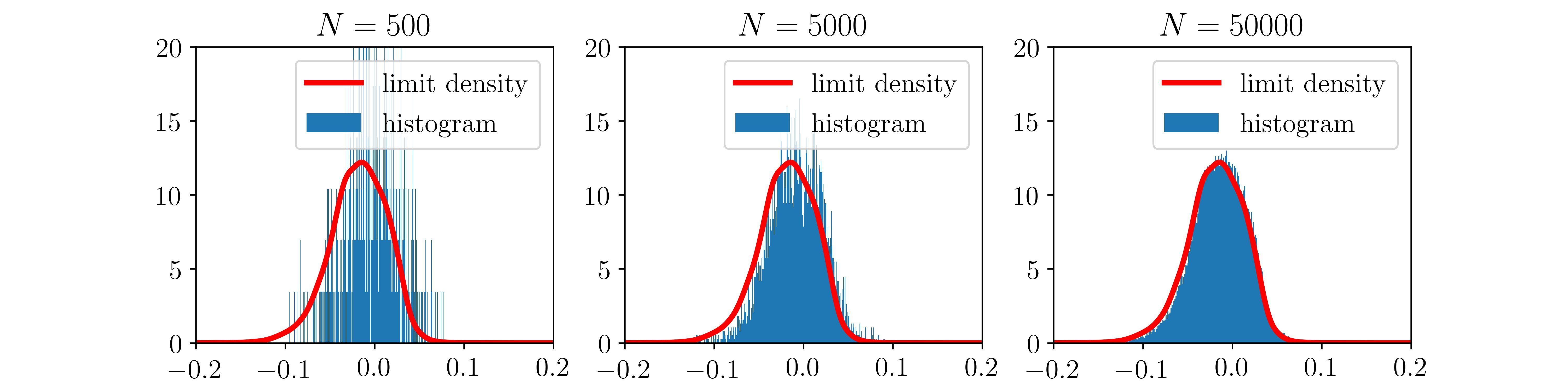
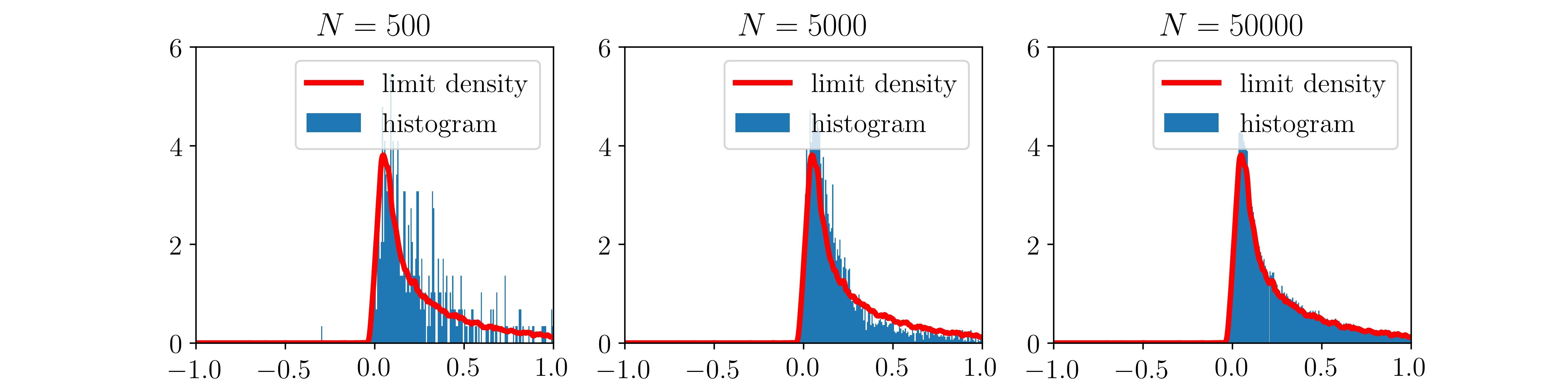
(a) Case $\alpha=0$

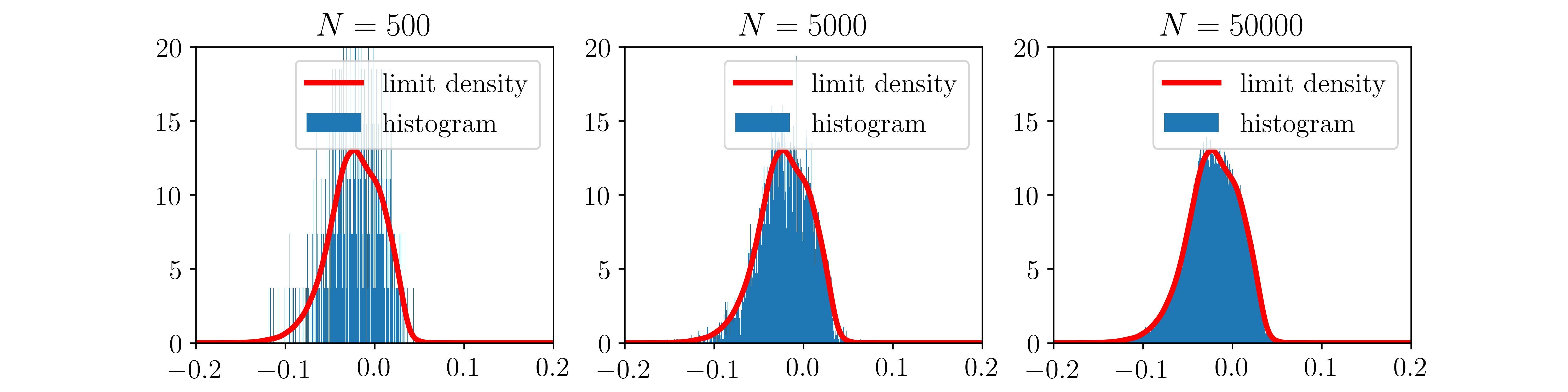
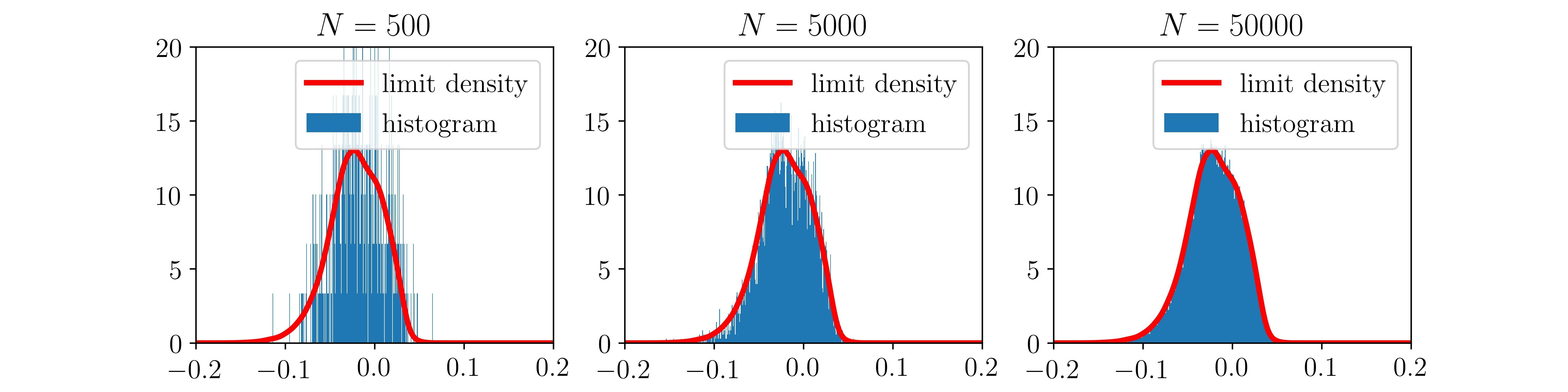
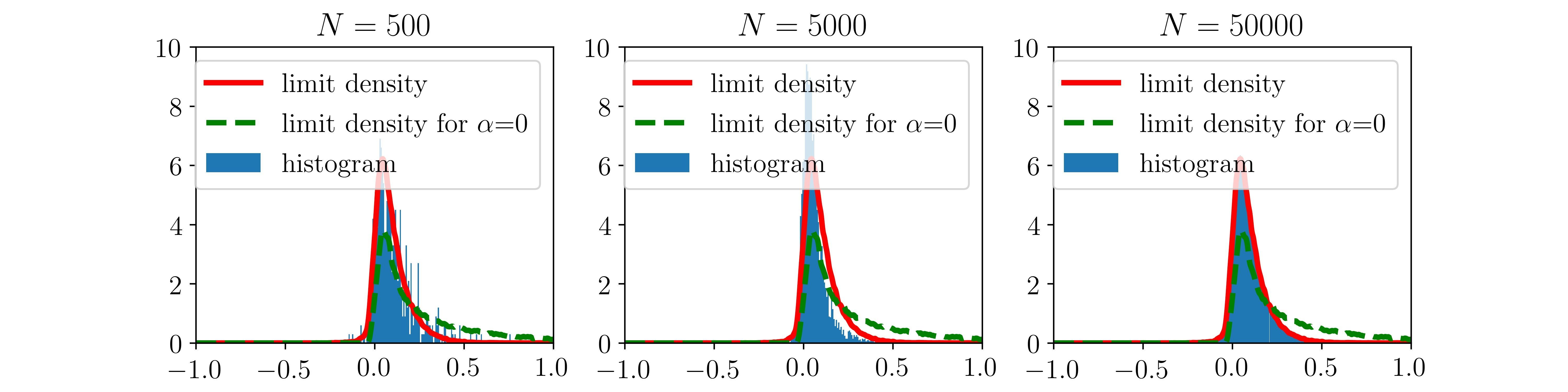
(b) Case $\alpha=0.25$

Figure 1: Convergence of the empirical distribution of the weights as $N\to+\infty$.

First we assess the convergence of the empirical distribution of the weights of the hidden layer to a limit distribution when $N\to+\infty$. We focus on the MNIST classification task. Note that in this case $p=28\times 28=784$. In Figure 1, we observe the behavior of the histograms of the weights $W_{n_{T}}^{1:N}$ of the hidden layer along the coordinate $(1,1)$ as $N\to+\infty$. We experimentally observe the existence of two different regimes, one for $\beta<1$ and the other one for $\beta=1$. In Figure 1, the first line corresponds to the evolution of the histogram in the case where $\beta=0.5$. The second and the third lines correspond to the same experiment with $\beta=0.75$ and $\beta=1$, respectively. Note that in both cases the histograms converge to a limit. This limit histogram exhibits two regimes depending if $\beta<1$ or $\beta=1$.

Existence of two regimes.

Figure 2: Deterministic versus stochastic behavior depending on the value $\beta$.

Now we assess the stochastic nature of the second regime we obtain in the case $\beta=1$ in contrast to the regime for $\beta<1$ which is deterministic. In order to highlight this situation, all the weights of the neural network are initialized with a fixed value, i.e., for any $N\in\mathbb{N}^{\star}$ and $k\in\{1,\ldots,N\}$, $W^{k,N}_{0}=w_{0}\in\mathbb{R}^{p}$. Then, the neural network is trained on the MNIST dataset for $N=10^{6}$ and $\beta=0.75$ or $\beta=1$. Figure 2 represents $7$ samples of the first component of $W_{n_{T}}^{1:N}$ obtained with independent runs of SGD. We can observe that for $\beta=0.75$ all the samples converge to the same value which agrees with (17) while in the case where $\beta=1$ they exhibit different values, which is in accordance with (19).

From stochastic to deterministic.

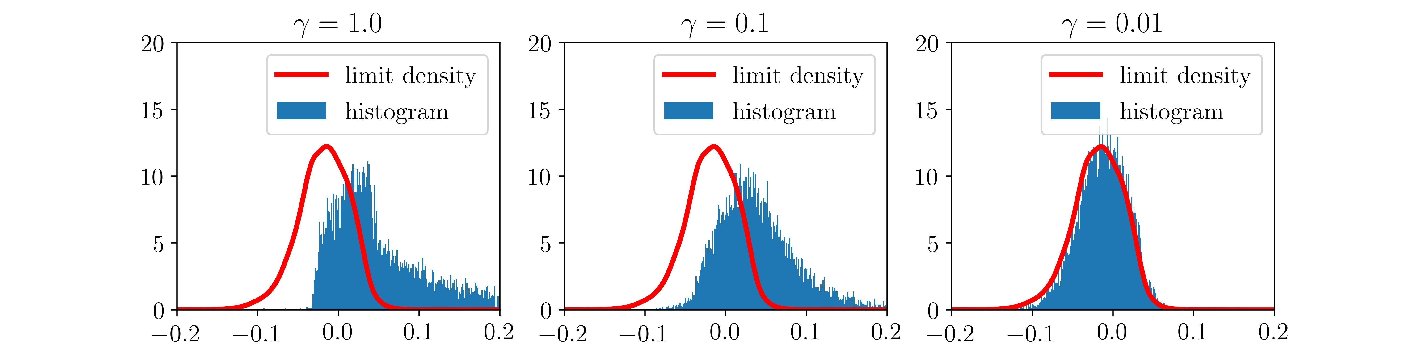
Figure 3: Convergence to the deterministic regime as $\gamma\to 0$.

We illustrate that when $\gamma\to 0$ the dynamics identified in (19) tends to the one identified in (17). We fix $\beta=1$ and $N=10000$ and focus on the MNIST classification task. In Figure 3 we show the histogram of the weights $W_{n_{T}}^{1:N}$ along the coordinate $(1,1)$ for different values of $\gamma$. As expected, see (19) and the following remark, when $\gamma\to 0$ we recover the limit histogram with $\beta<1$. In Figure 8 we also study the convergence of the empirical measure when $M\to+\infty$ in the case where $\beta<1$.

Long-time behavior.

Finally, we illustrate the interest of taking $\beta=1$ in our setting by considering the more challenging classification task on the CIFAR-10 dataset. We consider the following set of parameters $\alpha=0$, $M=100$, $T=10000$, $\gamma=0.1$. We emphasize that this experiment aims at comparing the performance of the setting $\beta<1$ and the one with $\beta=1$ and that we are not trying to reach state-of-the-art results. In Table 1 we present training and test accuracies for the classification task at hand. To build the classification estimator we average the weights along their trajectory, i.e., we perform averaging and consider the average estimator $\bar{W}_{n_{T}}^{1:N}=(n_{T}-n_{0}+1)^{-1}\sum_{n=n_{0}}^{n_{T}}W_{n}^{1:N}$, where $n_{0}=1000$. Using $\beta=1$ roughly increases the test accuracy by $1\%$, while the training accuracy is not $100\%$. This empirically seems to demonstrate that using a smaller value of $\beta$ tends to overfit the data, whereas using $\beta=1$ has a regularizing effect.

Table 1: Training and Test accuracies for different settings on the CIFAR-10 dataset, with $\alpha=0$, $M=100$ and $\gamma=0.1$ for $T=10000$

Values	$N=5000$	$N=5000$	$N=10000$	$N=10000$	$N=50000$	$N=50000$
of $N$ and $\beta$	$\beta=0.75$	$\beta=1.0$	$\beta=0.75$	$\beta=1.0$	$\beta=0.75$	$\beta=1.0$
Train acc.	100%	$97.2\%$	100%	$97.2\%$	100%	$99\%$
Test acc.	$55.5\%$	56.5%	$56.0\%$	56.5%	$56.7\%$	57.7%

5 Conclusion

We show in this paper that taking a stepsize in SGD depending on the number of hidden units leads to particle systems with two possible mean-field behaviours. The first was already identified in [22, 23, 28] and corresponds to a deterministic mean-field ODE. The second is new and corresponds to a McKean-Vlasov diffusion. Our numerical experiments on two real datasets support our findings. In a future work, we intend to follow the same approach for deep neural networks, i.e., with a growing number of hidden layers.

6 Preliminaries

6.1 Notation

Let $(\mathsf{E},d_{E})$ and $(\mathsf{F},d_{F})$ be two metric spaces. $\mathrm{C}(\mathsf{E},\mathsf{F})$ stands for the set of continuous $\mathsf{F}$-valued functions. If $\mathsf{F}=\mathbb{R}$, then we simply note $\mathrm{C}(\mathsf{E})$.

We say that $f:\ \mathsf{E}\to\mathbb{R}^{p}$ is $L$-Lipschitz if there exists $L\geq 0$ such that for any $x,y\in\mathsf{E}$, $\|f(x)-f(y)\|\leq Ld_{E}(x,y)$. Let $\mathrm{C}_{\mathrm{b}}(\mathsf{E},\mathbb{R}^{p})$ (respectively $\mathrm{C}_{\mathrm{c}}(\mathsf{E},\mathbb{R}^{p})$) be the set of bounded continuous functions from $\mathsf{E}$ to $\mathbb{R}^{p}$ (respectively the set of compactly supported functions from $\mathsf{E}$ to $\mathbb{R}^{p}$). If $p=1$, we simply note $\mathrm{C}_{\mathrm{b}}(\mathsf{E})$ (respectively $\mathrm{C}_{\mathrm{c}}(\mathsf{E})$).

For $\mathsf{U}$ an open set of $\mathbb{R}^{d}$, $n\in\mathbb{N}^{\star}$ and define $\mathrm{C}^{n}(\mathsf{U},\mathbb{R}^{p})$ the set of the $n$-differentiable $\mathbb{R}^{p}$-valued functions over $\mathsf{U}$. If $p=1$ then we simply note $\mathrm{C}^{n}(\mathsf{U})$. Let $f\in\mathrm{C}^{1}(\mathsf{U})$ we denote by $\nabla f$ its gradient. More generally, if $f\in\mathrm{C}^{n}(\mathsf{U},\mathbb{R}^{p})$ with $n,p\in\mathbb{N}^{\star}$, we denote by $\mathrm{D}^{k}f(x)$ the $k$-th differential of $f$. We also denote for any $i\in\{1,\dots,d\}$ and $\ell\in\{1,\dots,k\}$, $\partial_{i}^{\ell}f$ the $i$-th partial derivative of $f$ of order $\ell$. If $f\in\mathrm{C}^{2}(\mathbb{R}^{d},\mathbb{R})$, we denote by $\Delta f$ its Laplacian. $\mathrm{C}_{\mathrm{c}}^{n}(\mathsf{U},\mathbb{R}^{p})$ is the subset of $\mathrm{C}^{n}(\mathsf{U},\mathbb{R}^{p})$ such that for any $f\in\mathrm{C}_{\mathrm{c}}^{n}(\mathsf{U},\mathbb{R}^{p})$ and $\ell\in\{0,\dots,n\}$, $\mathrm{D}^{\ell}f$ has compact support.

Consider $(\mathsf{F},d)$ a metric space. Let $\mathscr{P}(\mathsf{F})$ be the space of probability measures over $\mathsf{F}$ equipped with its Borel $\sigma$-field $\mathcal{B}(\mathsf{F})$. For any $\mu\in\mathscr{P}(\mathsf{F})$ and $f:\ \mathsf{F}\to\mathbb{R}$, we say that $f$ is $\mu$-integrable if $\int_{\mathsf{F}}|f(x)|\mathrm{d}\mu(x)<+\infty$. In this case, we set $\mu[f]=\int_{\mathsf{F}}f(x)\mathrm{d}\mu(x)$. Let $\mu_{0}\in\mathscr{P}(\mathsf{F})$. For any $r\geq 1$, define $\mathscr{P}_{r}(\mathsf{F})=\{\mu\in\mathscr{P}(\mathsf{F})\,:\;\int_{\mathbb{R}^{p}}d(\mu_{0},\mu)^{r}\mathrm{d}\mu(x)<+\infty\}$. If not specified, we consider a filtered probability space $(\Omega,\mathcal{F},\mathbb{P},(\mathcal{F}_{t})_{t\geq 0})$ satisfying the usual conditions and any random variables is defined on this probability space. Let $f:\ (\mathsf{E},\mathcal{E})\to(\mathsf{G},\mathcal{G})$ be a measurable function. Then for any measure $\mu$ on $\mathcal{E}$ we define its pushforward measure by $f$, $f_{\#}\mu$, for any $\mathsf{A}\in\mathcal{G}$ by $f_{\#}\mu(\mathsf{A})=\mu(f^{-1}(\mathsf{A}))$.

The set of $m\times n$ real matrices is denoted by $\mathbb{R}^{m\times n}$. The set of symmetric real matrices of size $p$ is denoted $\mathbb{S}_{p}(\mathbb{R})$.

6.2 Wasserstein distances

Let $(\mathsf{F},d)$ be a metric space. Let $\mu_{1},\mu_{2}\in\mathscr{P}(\mathsf{F})$, where $\mathsf{F}$ is equipped with its Borel $\sigma$-field $\mathcal{B}(\mathsf{F})$. A probability measure $\zeta$ over $\mathcal{B}(\mathsf{F})^{\otimes 2}$ is said to be a transference plan between $\mu_{1}$ and $\mu_{2}$ if for any $\mathsf{A}\in\mathcal{B}(\mathsf{F})$, $\zeta(\mathsf{A}\times\mathsf{F})=\mu_{1}(\mathsf{A})$ and $\zeta(\mathsf{F}\times\mathsf{A})=\mu_{2}(\mathsf{A})$. We denote by $\Lambda(\mu_{1},\mu_{2})$ the set of all transference plans between $\mu_{1}$ and $\mu_{2}$. If $\mu_{1},\mu_{2}\in\mathscr{P}_{r}(\mathbb{R}^{p})$, we define the Wasserstein distance $\mathpzc{W}_{r}(\mu_{1},\mu_{2})$ of order $r$ between $\mu_{1}$ and $\mu_{2}$ by

$$\mathpzc{W}_{r}^{r}(\mu_{1},\mu_{2})=\inf_{\zeta\in\Lambda(\mu_{1},\mu_{2})}\left\{\int_{\mathsf{F}\times\mathsf{F}}d(x,y)^{r}\mathrm{d}\zeta(x,y)\right\}\;.$$ (24)

Note that $\mathpzc{W}_{r}$ is a distance on $\mathscr{P}_{r}(\mathsf{F})$ by [43, Theorem 6.18]. In addition $(\mathscr{P}_{r}(\mathbb{R}^{p}),\mathpzc{W}_{r})$ is a complete separable metric space. For any $\mu_{1},\mu_{2}\in\mathscr{P}_{p}(\mathsf{F})$ we say that a couple of random variables $(X,Y)$ is an optimal coupling of $(\mu_{1},\mu_{2})$ for $\mathpzc{W}_{p}$ if it has distribution $\xi$ where $\xi$ is an optimal transference plan between $\mu_{1}$ and $\mu_{2}$.

For any $T\geq 0$, the space $\mathscr{C}_{2,T}^{p}=\mathrm{C}(\left[0,T\right],\mathscr{P}_{2}(\mathbb{R}^{p}))$ is a complete separable metric space [44, Theorem 4.19] with the metric $\mathpzc{W}_{2,T}$ given for any $(\nu_{t})_{t\in\left[0,T\right]}$ and $(\mu_{t})_{t\in\left[0,T\right]}$ by

$$\mathpzc{W}_{2,T}((\nu_{t})_{t\in\left[0,T\right]},(\mu_{t})_{t\in\left[0,T\right]})=\sup_{t\in\left[0,T\right]}\mathpzc{W}_{2}(\nu_{t},\mu_{t})\;.$$ (25)

In the case where the measures we consider can be written as sums of Dirac we have the following proposition.

Proposition .

Let $r\geq 1$, $N\in\mathbb{N}^{\star}$, $\{\alpha_{k}\}_{k=1}^{N}\in\left[0,1\right]^{N}$ with $\sum_{k=1}^{N}\alpha_{k}=1$, $\{\mu_{k,a}\}_{k=1}^{N}\in\mathscr{P}(\mathsf{F})^{N}$ and $\{\mu_{k,b}\}_{k=1}^{N}\in\mathscr{P}(\mathsf{F})^{N}$. Then, setting $\nu_{i}=\sum_{k=1}^{N}\alpha_{k}\mu_{k,i}$ with $i\in\{a,b\}$, we have

$$\mathpzc{W}_{r}^{r}(\nu_{a},\nu_{b})w\leq\sum_{k=1}^{N}\mathpzc{W}_{r}^{r}(\mu_{k,a},\mu_{k,b})\;.$$ (26)

Proof.

Consider $\zeta=\sum_{k=1}^{N}\alpha_{k}\zeta_{k}\in\Lambda(\nu_{a},\nu_{b})$ with $\zeta_{k}$ the optimal transference plan between $\mu_{k,a}$ and $\mu_{k,b}$. Then, we have

$$\mathpzc{W}_{r}^{r}\left(\nu_{a},\nu_{b}\right)\leq\int_{\mathbb{R}^{p}\times\mathbb{R}^{p}}d(x,y)^{r}\mathrm{d}\zeta(x,y)\leq N^{-1}\sum_{k=1}^{N}\mathpzc{W}_{r}^{r}(\mu_{k,a},\mu_{k,b})\;.$$ (27)

∎

As a special case of Section 6.2, we obtain that for any $r\geq 1$, $\{w_{k,a}\}_{k=1}^{N}\in\mathsf{F}^{N}$ and $\{w_{k,a}\}_{k=1}^{N}\in\mathsf{F}^{N}$,

$$\mathpzc{W}_{r}(N^{-1}\sum_{k=1}^{N}\updelta_{w_{k,a}},N^{-1}\sum_{k=1}^{N}\updelta_{w_{k,b}})\leq N^{-1}\sum_{k=1}^{N}d(w_{k,a},w_{k,b})^{r}\;.$$ (28)

As another special case of Section 6.2, we obtain that for any $\mu\in\mathscr{P}_{r}(\mathsf{F})$ and $\{w_{k}\}_{k=1}^{N}\in\mathsf{F}^{N}$

$$\mathpzc{W}_{r}(N^{-1}\sum_{k=1}^{N}\updelta_{w_{k}},N^{-1},\mu)\leq N^{-1}\sum_{k=1}^{N}\mathpzc{W}_{r}(w_{k},\mu)^{r}\;.$$ (29)

7 A mean-field modification of Stochastic Gradient Langevin Dynamics

7.1 Presentation of the modified SGLD and its continuous counterpart

We start by introducing a modified Stochastic Gradient Langevin Dynamics (mSGLD) [39]. In the mean-field regime, this setting was studied in the case $\beta=0$ in [23]. We recall that the mean-field $h:\mathbb{R}^{p}\times\mathscr{P}(\mathbb{R}^{d})\to\mathbb{R}^{p}$ and $\xi:\mathbb{R}^{p}\times\mathscr{P}(\mathbb{R}^{d})\times\mathsf{X}\times\mathsf{Y}\to\mathbb{R}^{p}$ are given for any $\mu\in\mathscr{P}(\mathbb{R}^{p})$, $w\in\mathbb{R}^{p}$, $(x,y)\in\mathsf{X}\times\mathsf{Y}$ by

$$h(w,\mu)=-\int_{\mathsf{X}\times\mathsf{Y}}\partial_{1}\ell\left(\mu[F(\cdot,x)],y\right)\nabla_{w}F(w,x)\,\mathrm{d}\pi(x,y)-\nabla V(w)\;,$$ (30)

$$\xi(w,\mu,x,y)=-h(w,\mu)-\partial_{1}\ell(\mu[F(\cdot,x)],y)\nabla_{w}F(w,x)-\nabla V(w)\;.$$ (31)

Let $(W_{0}^{k})_{k\in\mathbb{N}^{\star}}$ be i.i.d. $p$ dimensional random variables with distribution $\mu_{0}$ and $\{Z_{k}^{n}\,:\;k,n\in\mathbb{N}^{\star}\}$ be i.i.d. $p$ dimensional independent Gaussian random variables with zero mean and identity covariance matrix. Consider the sequence $(W_{n}^{1:N})_{n\in\mathbb{N}}$ associated with mSGLD starting from $W_{0}^{1:N}$ and defined by the following recursion: for any $n\in\mathbb{N}$, $k\in\{1,\ldots,N\}$,

$$W^{k,N}_{n+1}=W^{k,N}_{n}+\gamma N^{\beta-1}(n+\gamma_{\alpha,\beta}(N)^{-1})^{-\alpha}\left\{h(W^{k,N}_{n},\nu_{n}^{N})+\xi(W^{k,N}_{n},\nu_{n}^{N},X_{n},Y_{n})\right\}\\ +\left[2\eta\gamma N^{\beta-1}(n+\gamma_{\alpha,\beta}(N)^{-1})^{-\alpha}\right]^{1/2}Z_{k,n}\;,$$ (32)

where $\eta\geq 0$, $\beta\in\left[0,1\right]$, $\alpha\in\left[0,1\right)$, $\gamma>0$, $(X_{n},Y_{n})_{n\in\mathbb{N}}$ is a sequence of i.i.d. input/label samples distributed according to $\pi$ and $\gamma_{\alpha,\beta}(N)=\gamma^{1/(1-\alpha)}N^{(\beta-1)/(1-\alpha)}$. Note that in the cas $\eta=0$, we obtain (8). In addition, (32) does not exactly correspond to the usual implementation of mSGLD as introduced in [39]. Indeed, to recover this algorithm, we should replace $[2\eta\gamma N^{\beta-1}(n+\gamma_{\alpha,\beta}(N)^{-1})^{-\alpha}]^{1/2}Z_{k,n}$ by $[2\eta\gamma N^{\beta}(n+\gamma_{\alpha,\beta}(N)^{-1})^{-\alpha}]^{1/2}Z_{k,n}$ in (32). The scheme presented in (32) amounts to consider a temperature which scales as $\gamma N^{\beta-1}$ with the number of particles. As emphasized before, this scheme was also considered in [23].

We now present the continuous model associated with this discrete process in the limit $\gamma\to 0$ or $N\to+\infty$. For $N\in\mathbb{N}^{\star}$, consider the particle system diffusion $(\mathbf{W}^{1:N}_{t})_{t\geq 0}=(\{\mathbf{W}^{k,N}_{t}\}_{k=1}^{N})_{t\geq 0}$ starting from $\mathbf{W}^{1:N}_{0}$ defined for any $k\in\{1,\dots,N\}$ by

$$\mathrm{d}\mathbf{W}^{k,N}_{t}=(t+1)^{-\alpha}\left\{h(\mathbf{W}^{k,N}_{t},\bm{\nu}^{N}_{t})\mathrm{d}t+\gamma_{\alpha,\beta}(N)^{1/2}\Sigma^{1/2}(\mathbf{W}^{k,N}_{t},\bm{\nu}^{N}_{t})\mathrm{d}\mathbf{B}^{k}_{t}+\sqrt{2\eta}\mathrm{d}\tilde{\mathbf{B}}_{t}^{k}\right\}\;,$$ (33)

where $\{(\mathbf{B}_{t}^{k})_{t\geq 0}\,:\;k\in\mathbb{N}^{\star}\}$ and $\{(\tilde{\mathbf{B}}_{t}^{k})_{t\geq 0}\,:\;k\in\mathbb{N}^{\star}\}$ are two independent families of independent $p$ dimensional Brownian motions and $\bm{\nu}^{N}_{t}$ is the empirical probability distribution of the particles defined for any $t\geq 0$ by $\bm{\nu}^{N}_{t}=N^{-1}\sum_{k=1}^{N}\updelta_{\mathbf{W}^{k,N}_{t}}$. Similarly to Section 2, (33) is the continuous counterpart of (32). Let $M\in\mathbb{N}^{\star}$. Similarly to (16), we consider the following particle system diffusion $(\mathbf{W}^{1:N}_{t})_{t\geq 0}=(\{\mathbf{W}^{k,N}_{t}\}_{k=1}^{N})_{t\geq 0}$ starting from $\mathbf{W}^{1:N}_{0}$ defined for any $k\in\{1,\dots,N\}$ by

$$\mathrm{d}\mathbf{W}^{k,N}_{t}=(t+1)^{-\alpha}\left\{h(\mathbf{W}^{k,N}_{t},\bm{\nu}^{N}_{t})\mathrm{d}t+(\gamma_{\alpha,\beta}(N)/M)^{1/2}\Sigma^{1/2}(\mathbf{W}^{k,N}_{t},\bm{\nu}^{N}_{t})\mathrm{d}\mathbf{B}^{k}_{t}+\sqrt{2\eta}\mathrm{d}\tilde{\mathbf{B}}_{t}^{k}\right\}\;.$$ (34)

7.2 Mean field approximation and propagation of chaos for mSGLD

The following theorems are the extensions of Theorem 1 and Theorem 2 to (33) for any $\eta\geq 0$. Note that in the case $\eta=0$, Theorem 3 boils down to Theorem 1 and Theorem 4 to Theorem 2.

We start by stating our results in the case $\beta\in\left[0,1\right)$. Consider the mean-field SDE starting from a random variable $\mathbf{W}_{0}^{\star}$ given by

$$\mathrm{d}\mathbf{W}_{t}^{\star}=(t+1)^{-\alpha}\left\{h(\mathbf{W}_{t}^{\star},\bm{\lambda}_{t}^{\star})\mathrm{d}t+\sqrt{2\eta}\tilde{\mathbf{B}}_{t}\right\}\;,\qquad\text{with $\bm{\lambda}^{\star}_{t}$ the distribution of $\mathbf{W}_{t}^{\star}$}\;.$$ (35)

Theorem 3.

Assume 1. Let $(\mathbf{W}_{0}^{k})_{k\in\mathbb{N}}$ be a sequence of i.i.d. $\mathbb{R}^{p}$-valued random variables with distribution $\mu_{0}\in\mathscr{P}_{2}(\mathbb{R}^{p})$ and set for any $N\in\mathbb{N}^{\star}$, $\mathbf{W}_{0}^{1:N}=\{\mathbf{W}_{0}^{k}\}_{k=1}^{N}$. Then, for any $m\in\mathbb{N}^{\star}$ and $T\geq 0$, there exists $C_{m,T}\geq 0$ such that for any $\alpha\in\left[0,1\right)$, $\beta\in\left[0,1\right)$, $M\in\mathbb{N}^{\star}$ and $N\in\mathbb{N}^{\star}$

$$\textstyle{\mathbb{E}\left[\sup_{t\in\left[0,T\right]}\|\mathbf{W}_{t}^{1:m,N}-\mathbf{W}_{t}^{1:m,\star}\|^{2}\right]\leq C_{m,T}\left\{N^{-(1-\beta)/(1-\alpha)}M^{-1}+N^{-1}\right\}\;,}$$ (36)

with $(\mathbf{W}_{t}^{1:m,N},\mathbf{W}_{t}^{1:m,\star})=\{(\mathbf{W}_{t}^{k,N},\mathbf{W}_{t}^{k,\star})\}_{k=1}^{m}$, $(\mathbf{W}_{t}^{1:N})$ is the solution of (34) starting from $\mathbf{W}_{0}^{1:N}$, and for any $k\in\{1,\ldots,N\}$, $\mathbf{W}_{t}^{k,\star}$ is the solution of (35) starting from $\mathbf{W}_{0}^{k}$ and Brownian motion $(\tilde{\mathbf{B}}^{k}_{t})_{t\geq 0}$.

Proof.

The proof is postponed to Section 9.4 ∎

Consider now the mean-field SDE starting from a random variable $\mathbf{W}_{0}^{\star}$ given by

$$\mathrm{d}\mathbf{W}_{t}^{\star}=(t+1)^{-\alpha}\left\{h(\mathbf{W}_{t}^{\star},\bm{\lambda}_{t}^{\star})\mathrm{d}t+(\gamma^{1/(1-\alpha)}\Sigma(\mathbf{W}_{t}^{\star},\bm{\lambda}_{t}^{\star})/M)^{1/2}\mathrm{d}\mathbf{B}_{t}+\sqrt{2\eta}\mathrm{d}\tilde{\mathbf{B}}_{t}\right\}\;,$$ (37)

where $\bm{\lambda}^{\star}_{t}$ is the distribution of $\mathbf{W}_{t}^{\star}$ and $(\mathbf{B}_{t})_{t\geq 0}$ and $(\tilde{\mathbf{B}}_{t})_{t\geq 0}$ are independent $p$ dimensional Brownian motions.

Theorem 4.

Let $\beta=1$. Assume 1. Let $(\mathbf{W}_{0}^{k})_{k\in\mathbb{N}}$ be a sequence of $\mathbb{R}^{p}$-valued random variables with distribution $\mu_{0}\in\mathscr{P}_{2}(\mathbb{R}^{p})$ and assume that for any $N\in\mathbb{N}^{\star}$, $\mathbf{W}_{0}^{1:N}=\{\mathbf{W}_{0}^{k}\}_{k=1}^{N}$. Then, for any $m\in\mathbb{N}^{\star}$ and $T\geq 0$, there exists $C_{m,T}\geq 0$ such that for any $\alpha\in\left[0,1\right)$, $M\in\mathbb{N}^{\star}$ and $N\in\mathbb{N}^{\star}$ we have

$$\textstyle{\mathbb{E}\left[\sup_{t\in\left[0,T\right]}\|\mathbf{W}_{t}^{1:m,N}-\mathbf{W}_{t}^{1:m,\star}\|^{2}\right]\leq C_{m,T}N^{-1}\;,}$$ (38)

with $(\mathbf{W}_{t}^{1:m,N},\mathbf{W}_{t}^{1:m,\star})=\{(\mathbf{W}_{t}^{k,N},\mathbf{W}_{t}^{k,\star})\}_{k=1}^{m}$, $(\mathbf{W}_{t}^{1:N})$ is the solution of (34) starting from $\mathbf{W}_{0}^{1:N}$, and for any $k\in\{1,\ldots,N\}$, $\mathbf{W}_{t}^{k,\star}$ is the solution of (37) starting from $\mathbf{W}_{0}^{k}$ and Brownian motions $(\mathbf{B}^{k}_{t})_{t\geq 0}$ and $(\tilde{\mathbf{B}}^{k}_{t})_{t\geq 0}$.

Proof.

The proof is postponed to Section 9.4 ∎

8 Technical results

In this section, we derive technical results needed to establish Theorem 1, Theorem 2, Theorem 3 and Theorem 4. In particular, we are interested in the regularity properties of the mean field $h$ and the diffusion matrix $\Sigma$ under 1. We recall that in this setting, for any $w\in\mathbb{R}^{p}$, $\mu\in\mathscr{P}(\mathbb{R}^{p})$, $(x,y)\in\mathsf{X}\times\mathsf{Y}$, we have

$$h(w,\mu) =\tilde{h}(w,\mu)-\nabla V(w)\;,$$ (39)

$$\text{ with }\quad\tilde{h}(w,\mu) =-\int_{\mathsf{X}\times\mathsf{Y}}\partial_{1}\ell\left(\int_{\mathbb{R}^{p}}F(\zeta,x)\,\mathrm{d}\mu(\zeta),y\right)\nabla_{w}F(w,x)\,\mathrm{d}\pi(x,y)\;,$$ (40)

$$\xi(w,\mu,x,y) =-\tilde{h}(w,\mu)-\partial_{1}\ell\left(\int_{\mathbb{R}^{p}}F(\zeta,x)\,\mathrm{d}\mu(\zeta),y\right)\nabla_{w}F(w,x)\;,$$ (41)

$$\Sigma(w,\mu) =\int_{\mathsf{X}\times\mathsf{Y}}\{\xi\xi^{\top}\}(w,\mu,x,y)\mathrm{d}\pi(x,y)\;,\qquad\mathrm{S}(w,\mu)=\Sigma^{1/2}(w,\mu)\;.$$ (42)

Note that by 1-(a), we obtain the following estimate used in the proof of the results of this Section: for any $\mathrm{y},y\in\mathbb{R}$

$$\left|\partial_{1}\ell(\mathrm{y},y)\right|\leq\left|\partial_{1}\ell(0,y)\right|+\Psi(y)\left|\mathrm{y}\right|\leq 2\Psi(y)\max(1,\left|\mathrm{y}\right|)\;.$$ (43)

In addition, note that under 1-(c), there exists $\mathtt{K}\geq 0$ such that for any $w\in\mathbb{R}^{p}$

$$\left\|\nabla^{2}V(w)\right\|+\left\|\mathrm{D}^{3}V(w)\right\|\leq\mathtt{K}\;,\qquad\left\|\nabla V(w)\right\|\leq\mathtt{K}(1+\left\|w\right\|)\;.$$ (44)

Let $G:\ \mathbb{R}^{p}\times\mathsf{X}\times\mathsf{Y}\to\mathbb{R}$ given for any $(x,y)\in\mathsf{X}\times\mathsf{Y}$ and $w\in\mathbb{R}^{p}$ by

$$G(w,x,y)=\{\Phi^{4}(x)+\Psi^{2}(y)\}F(w,x)\;.$$ (45)

We now state our main regularity/boundedness proposition.

Proposition .

Assume 1. Then, there exists $\mathtt{L}\geq 0$ such that the following hold.

1. For any $\mu_{1},\mu_{2}\in\mathscr{P}(\mathbb{R}^{p})$ and $w_{1},w_{2}\in\mathbb{R}^{p}$ we have

   $$\left\|h(w_{1},\mu_{1})-h(w_{2},\mu_{2})\right\|\\ \leq\mathtt{L}\left\{\left\|w_{1}-w_{2}\right\|+\left(\int_{\mathsf{X}\times\mathsf{Y}}\left\|\mu_{1}[G(\cdot,x,y)]-\mu_{2}[G(\cdot,x,y)]\right\|^{2}\mathrm{d}\pi(x,y)\right)^{1/2}\right\}\;.$$ (46)

   In addition, we have for any $\mu\in\mathscr{P}(\mathbb{R}^{p})$ and $w\in\mathbb{R}^{p}$, $\|h(w,\mu)\|\leq\mathtt{L}(1+\|w\|)$ and $\|\bar{h}(w,\mu)\|\leq\mathtt{L}$.

2. For any $\mu_{1},\mu_{2}\in\mathscr{P}(\mathbb{R}^{p})$, $w_{1},w_{2}\in\mathbb{R}^{p}$ and $i,j\in\{1,\dots,p\}$ we have

   $$\left|\mathrm{S}_{i,j}(w_{1},\mu_{1})-\mathrm{S}_{i,j}(w_{2},\mu_{2})\right|\\ \leq\mathtt{L}\left\{\left\|w_{1}-w_{2}\right\|+\left(\int_{\mathsf{X}\times\mathsf{Y}}\left\|\mu_{1}[G(\cdot,x,y)]-\mu_{2}[G(\cdot,x,y)]\right\|^{2}\mathrm{d}\pi(x,y)\right)^{1/2}\right\}\;.$$ (47)

   In addition, we have for any $\mu\in\mathscr{P}(\mathbb{R}^{p})$, $w\in\mathbb{R}^{p}$ and $i,j\in\{1,\dots,p\}$, $|\mathrm{S}_{i,j}(w,\mu)|\leq\mathtt{L}$.

3. For any $\mu\in\mathscr{P}(\mathbb{R}^{p})$ and $w\in\mathbb{R}^{p}$, $\int_{\mathsf{X}\times\mathsf{Y}}\left\|\xi(w,\mu,x,y)\right\|^{2}\mathrm{d}\pi(x,y)\leq p^{2}\mathtt{L}^{2}$.

Proof.

1. First, we show that (46) holds. Note that by the triangle inequality and (42), we only need to consider $h\leftarrow\tilde{h}$ and $h\leftarrow V$. The case $h\leftarrow V$ is straightforward using (44). We now deal with the first case. For any $w_{1},w_{2}\in\mathbb{R}^{p}$ and $\mu_{1},\mu_{2}\in\mathscr{P}(\mathbb{R}^{p})$, consider the decomposition,

   $$\|\tilde{h}(w_{1},\mu_{1})-\tilde{h}(w_{2},\mu_{2})\|\leq\|\tilde{h}(w_{1},\mu_{1})-\tilde{h}(w_{2},\mu_{1})\|+\|\tilde{h}(w_{2},\mu_{1})-\tilde{h}(w_{2},\mu_{2})\|\;.$$ (48)

   In what follows, we bound separately the two terms in the right-hand side. Using 1-(a), 1-(b), (42) and (43) we have for any $w_{1},w_{2}\in\mathbb{R}^{p}$ and $\mu_{1}\in\mathscr{P}(\mathbb{R}^{p})$

   $$\|\tilde{h}(w_{1},\mu_{1})-\tilde{h}(w_{2},\mu_{1})\| \leq\left\|\int_{\mathsf{X}\times\mathsf{Y}}\partial_{1}\ell(\mu_{1}[F(\cdot,x)],y)\nabla_{w}F(w_{1},x)\,\mathrm{d}\pi(x,y)\right.$$ (49)

   $$\qquad\left.-\int_{\mathsf{X}\times\mathsf{Y}}\partial_{1}\ell(\mu_{1}[F(\cdot,x)],y)\nabla_{w}F(w_{2},x)\,\mathrm{d}\pi(x,y)\right\|$$ (50)

   $$\leq\int_{\mathsf{X}\times\mathsf{Y}}\left|\partial_{1}\ell(\mu_{1}[F(\cdot,x)],y)\right|\Phi(x)\mathrm{d}\pi(x,y)\left\|w_{1}-w_{2}\right\|$$ (51)

   $$\leq\int_{\mathsf{X}\times\mathsf{Y}}\Psi(y)\Phi(x)\left(1+\left|\mu_{1}[F(\cdot,x)]\right|\right)\mathrm{d}\pi(x,y)\left\|w_{1}-w_{2}\right\|$$ (52)

   $$\leq 2\int_{\mathsf{X}\times\mathsf{Y}}\Psi(y)\Phi^{2}(x)\mathrm{d}\pi(x,y)\left\|w_{1}-w_{2}\right\|\;.$$ (53)

   Using 1-(a), 1-(b), (42) and the Cauchy-Schwarz inequality, we also have for any $w_{1}\in\mathbb{R}^{p}$ and $\mu_{1},\mu_{2}\in\mathscr{P}(\mathbb{R}^{p})$

   $$\|\tilde{h}(\mu_{1},w_{1})-\tilde{h}(\mu_{2},w_{1})\|$$ (54)

   $$\qquad\leq\left\|\int_{\mathsf{X}\times\mathsf{Y}}\{\partial_{1}\ell(\mu_{1}[F(\cdot,x)],y)\nabla_{w}F(w_{1},x)-\partial_{1}\ell(\mu_{2}[F(\cdot,x)],y)\nabla_{w}F(w_{1},x)\}\,\mathrm{d}\pi(x,y)\right\|$$ (55)

   $$\qquad\leq\int_{\mathsf{X}\times\mathsf{Y}}\left|\partial_{1}\ell(\mu_{1}[F(\cdot,x)],y)-\partial_{1}\ell(\mu_{2}[F(\cdot,x)],y)\right|\left\|\nabla_{w}F(w_{1},x)\right\|\mathrm{d}\pi(x,y)$$ (56)

   $$\qquad\leq\int_{\mathsf{X}\times\mathsf{Y}}\Psi(y)\left\|\mu_{1}[F(\cdot,x)]-\mu_{2}[F(\cdot,x)]\right\|\Phi(x)\mathrm{d}\pi(x,y)$$ (57)

   $$\qquad\leq\left(\int_{\mathsf{X}\times\mathsf{Y}}\Psi^{2}(y)\Phi^{2}(x)\mathrm{d}\pi(x,y)\right)^{1/2}\left(\int_{\mathsf{X}}\left\|\mu_{1}[F(\cdot,x)]-\mu_{2}[F(\cdot,x)]\right\|^{2}\mathrm{d}\pi(x)\right)^{1/2}\;.$$ (58)

   Combining (45), (53), (58), the fact that for any $a,b\geq 0$, $2ab\leq a^{2}+b^{2}$ and 1-(d), we obtain that there exists $\mathtt{L}_{1}\geq 0$ such that for any $\mu_{1},\mu_{2}\in\mathscr{P}(\mathbb{R}^{p})$ and $w_{1},w_{2}\in\mathbb{R}^{p}$ we have

   $$\|\tilde{h}(w_{1},\mu_{1})-\tilde{h}(w_{2},\mu_{2})\|\\ \leq\mathtt{L}_{1}\left\{\left\|w_{1}-w_{2}\right\|+\left(\int_{\mathsf{X}\times\mathsf{Y}}\left\|\mu_{1}[G(\cdot,x,y)]-\mu_{2}[G(\cdot,x,y)]\right\|^{2}\mathrm{d}\pi(x,y)\right)^{1/2}\right\}\;.$$ (59)

   In addition, using 1-(b) and (43), we have for any $w\in\mathbb{R}^{p}$, $\mu\in\mathscr{P}(\mathbb{R}^{p})$, $x\in\mathsf{X}$ and $y\in\mathsf{Y}$

   $$\left|\partial_{1}\ell(\mu[F(\cdot,x)],y)\right|\left\|\nabla_{w}F(w,x)\right\|\leq\Psi(y)\Phi(x)(1+\Phi(x))\leq 2\Psi(y)\Phi^{2}(x)\;.$$ (60)

   Therefore, combining this result and (42), we get that for any $w\in\mathbb{R}^{p}$ and $\mu\in\mathscr{P}(\mathbb{R}^{p})$

   $$\|\tilde{h}(w,\mu)\|\leq\int_{\mathsf{X}\times\mathsf{Y}}2\Psi(y)\Phi^{2}(x)\mathrm{d}\pi(x,y)\;.$$ (61)

   Using the fact that for any $a,b\geq 0$, $2ab\leq a^{2}+b^{2}$ and 1-(d), there exists $\mathtt{L}_{2}\geq 0$ such that for any $w\in\mathbb{R}^{p}$ and $\mu\in\mathscr{P}(\mathbb{R}^{p})$,

   $$\|\tilde{h}(w,\mu)\|\leq\mathtt{L}_{2}$$ (62)

2. Second, we first show that there exists $\mathtt{L}_{3}\geq 0$ such that for any $\mu\in\mathscr{P}(\mathbb{R}^{p})$, $w\in\mathbb{R}^{p}$ and $i,j\in\{1,\dots,p\}$, $|\mathrm{S}_{i,j}(w,\mu)|\leq\mathtt{L}$. Let $i,j\in\{1,\dots,p\}$. We have for any $w\in\mathbb{R}^{p}$ and $\mu\in\mathscr{P}(\mathbb{R}^{p})$

   $$\left|\mathrm{S}_{i,j}(w,\mu)\right|\leq\|\mathrm{S}(w,\mu)\|\leq\operatorname{Tr}^{1/2}\left(\Sigma(w,\mu)\right)\;.$$ (63)

   Similarly to (60), using (42), (62), the fact that for any $a,b\geq 0$, $(a+b)^{2}\leq 2(a^{2}+b^{2})$ and the Cauchy-Schwarz inequality, we get for any $w\in\mathbb{R}^{p}$ and $\mu\in\mathscr{P}(\mathbb{R}^{p})$

   $$\operatorname{Tr}\left(\Sigma(w,\mu)\right)\leq\int_{\mathsf{X}\times\mathsf{Y}}\left\|\xi(w,\mu,x,y)\right\|^{2}\mathrm{d}\pi(x,y)\leq 2\int_{\mathsf{X}\times\mathsf{Y}}\{\mathtt{L}_{2}^{2}+2\Psi^{2}(y)\Phi^{4}(x)\}\mathrm{d}\pi(x,y)\;.$$ (64)

   Combining (63), (64) and 1-(d), there exists $\mathtt{L}_{3}\geq 0$ such that for any $w\in\mathbb{R}^{p}$ and $\mu\in\mathscr{P}(\mathbb{R}^{p})$, $\max_{1\leq i,j\leq p}|\mathrm{S}_{i,j}(w,\mu)|\leq\mathtt{L}_{3}$.

   We now show that (47) holds. For any $w_{1},w_{2}\in\mathbb{R}^{p}$, $\mu_{1},\mu_{2}\in\mathscr{P}(\mathbb{R}^{p})$ define $\varphi_{\Sigma}:\left[0,1\right]\to\mathbb{S}_{p}(\mathbb{R})$ for any $t\in\left[0,1\right]$ by

   $$\varphi_{\Sigma}(t)=\Sigma(tw_{1}+(1-t)w_{2},t\mu_{1}+(1-t)\mu_{2})\;.$$ (65)

   For ease of notation, the dependency of $\varphi_{\Sigma}$ with respect to $w_{1},w_{2}\in\mathbb{R}^{p}$ and $\mu_{1},\mu_{2}\in\mathscr{P}(\mathbb{R}^{p})$ is omitted. In what follows, we show that for any $w_{1},w_{2}\in\mathbb{R}^{p}$, $\mu_{1},\mu_{2}\in\mathscr{P}(\mathbb{R}^{p})$, $\varphi_{\Sigma}\in\mathrm{C}^{2}(\left[0,1\right],\mathbb{S}_{p}(\mathbb{R}))$ and that there exists $\mathtt{L}_{4}\geq 0$ such that for any $t\in\left[0,1\right]$

   $$\left\|\varphi_{\Sigma}^{\prime\prime}(t)\right\|\leq\mathtt{L}_{4}\left\{\left\|w_{1}-w_{2}\right\|+\left(\int_{\mathsf{X}\times\mathsf{Y}}\left\|\mu_{1}[G(\cdot,x,y)]-\mu_{2}[G(\cdot,x,y)]\right\|^{2}\mathrm{d}\pi(x,y)\right)^{1/2}\right\}^{2}\;,$$ (66)

   which will conclude the proof of (47) upon using a straightforward adaptation of [45, Lemma 3.2.3, Theorem 5.2.3]. We conclude the proof of Section 8 upon letting $\mathtt{L}=\max(\mathtt{L}_{1},\mathtt{L}_{2},\mathtt{L}_{3},\mathtt{L}_{4})$.

   For any $t\in\left[0,1\right]$, let $\mu_{t}=\mu_{1}+t(\mu_{2}-\mu_{1})\in\mathscr{P}(\mathbb{R}^{p})$ and $w_{t}=w_{1}+t(w_{2}-w_{1})\in\mathbb{R}^{p}$ and for any $(x,y)\in\mathsf{X}\times\mathsf{Y}$ define

   $$\mathrm{f}(t,x,y)=\partial_{1}\ell(\mu_{t}[F(\cdot,x)],y)\nabla_{w}F(w_{t},x)\;,$$ (67)

   $$\tilde{\mathrm{f}}(t,x,y)=\xi(w_{t},\mu_{t},x,y)=\int_{\mathsf{X}\times\mathsf{Y}}\mathrm{f}(t,x,y)\mathrm{d}\pi(x,y)-\mathrm{f}(t,x,y)\;.$$

   The rest of the proof consists in showing that $\varphi_{\Sigma}$ is twice differentiable with dominated derivatives using the Lebesgue convergence theorem.

   By (42), (60) and (62), we get that for any $w_{1},w_{2}\in\mathbb{R}^{p}$, $\mu_{1},\mu_{2}\in\mathscr{P}(\mathbb{R}^{p})$, $(x,y)\in\mathsf{X}\times\mathsf{Y}$ and $t\in\left[0,1\right]$

   $$\left\|\mathrm{f}(t,x,y)\right\|\leq 2\Psi(y)\Phi^{2}(x)\;,\qquad\|\tilde{\mathrm{f}}(t,x,y)\|\leq\mathtt{L}_{2}+2\Psi(y)\Phi^{2}(x)\;.$$ (68)

   Using (67), 1-(a) and 1-(b), we have that for any $(x,y)\in\mathsf{X}\times\mathsf{Y}$, $\mathrm{f}(\cdot,x,y)\in\mathrm{C}^{1}(\left[0,1\right],\mathbb{R}^{p})$ and for any $w_{1},w_{2}\in\mathbb{R}^{p}$, $\mu_{1},\mu_{2}\in\mathscr{P}(\mathbb{R}^{p})$, $(x,y)\in\mathsf{X}\times\mathsf{Y}$ and $t\in\left[0,1\right]$

   $$\partial_{1}\mathrm{f}(t,x,y)=\partial_{1}^{2}\ell(\mu_{t}[F(\cdot,x)],y)\nabla_{w}F(w_{t},x)\left(\mu_{2}[F(\cdot,x)]-\mu_{1}[F(\cdot,x)]\right)\\ +\partial_{1}\ell(\mu_{t}[F(\cdot,x)],y)\nabla_{w}^{2}F(w_{t},x)(w_{2}-w_{1})\;.$$ (69)

   Using 1-(a), 1-(b), (45) and (43), we get that for any $(x,y)\in\mathsf{X}\times\mathsf{Y}$ and $t\in\left[0,1\right]$

   $$\left\|\partial_{1}\mathrm{f}(t,x,y)\right\|\leq 3\Psi(y)\Phi^{2}(x)\left(\left\|w_{2}-w_{1}\right\|+\left\|\mu_{1}[F(\cdot,x)]-\mu_{2}[F(\cdot,x)]\right\|\right)\;,$$ (70)

   Similarly, using (69), 1-(a) and 1-(b), we have that for any $(x,y)\in\mathsf{X}\times\mathsf{Y}$, $\mathrm{f}(\cdot,x,y)\in\mathrm{C}^{2}(\left[0,1\right],\mathbb{R}^{p})$ and for any $w_{1},w_{2}\in\mathbb{R}^{p}$, $\mu_{1},\mu_{2}\in\mathscr{P}(\mathbb{R}^{p})$, $(x,y)\in\mathsf{X}\times\mathsf{Y}$ and $t\in\left[0,1\right]$

   $$\partial_{1}^{2}\mathrm{f}(t,x,y)=\partial_{1}^{3}\ell(\mu_{t}[F(\cdot,x)],y)\nabla_{w}F(w_{t},x)\left(\mu_{2}[F(\cdot,x)]-\mu_{1}[F(\cdot,x)]\right)^{2}\\ +2\partial_{1}^{2}\ell(\mu_{t}[F(\cdot,x)],y)\nabla_{w}^{2}F(w_{t},x)(w_{2}-w_{1})\left(\mu_{2}[F(\cdot,x)]-\mu_{1}[F(\cdot,x)]\right)\\ +\partial_{1}\ell(\mu_{t}[F(\cdot,x)],y)\mathrm{D}_{w}^{3}F(w_{t},x)(w_{2}-w_{1})^{\otimes 2}\;.$$ (71)

   Using 1-(a), 1-(b) and (43) and that for any $a,b\geq 0$, $2ab\leq a^{2}+b^{2}$, we get that for any $(x,y)\in\mathsf{X}\times\mathsf{Y}$ and $t\in\left[0,1\right]$

   $$\left\|\partial_{1}^{2}\mathrm{f}(t,x,y)\right\|\leq 5\Psi(y)\Phi^{2}(x)\left(\left\|w_{2}-w_{1}\right\|^{2}+\left\|\mu_{1}[F(\cdot,x)]-\mu_{2}[F(\cdot,x)]\right\|^{2}\right)\;.$$ (72)

   Combining (67), (70), (72), 1-(d) and the dominated convergence theorem, we get that for any $(x,y)\in\mathsf{X}\times\mathsf{Y}$, $\tilde{\mathrm{f}}(\cdot,x,y)\in\mathrm{C}^{2}(\left[0,1\right],\mathbb{R}^{p})$. In addition, using (67), (68), (70), (72), the Cauchy-Schwarz inequality and the fact that for any $a,b\geq 0$, $2ab\leq a^{2}+b^{2}$, there exists $C\geq 0$, such that for any $w_{1},w_{2}\in\mathbb{R}^{p}$, $\mu_{1},\mu_{2}\in\mathscr{P}(\mathbb{R}^{p})$, $(x,y)\in\mathsf{X}\times\mathsf{Y}$ and $t\in\left[0,1\right]$

   $$\|\tilde{\mathrm{f}}(t,x,y)\| \leq C\left(\Phi^{4}(x)+\Psi^{2}(y)\right)\;,$$ (73)

   $$\|\partial_{1}\tilde{\mathrm{f}}(t,x,y)\| \leq C\left(\Phi^{4}(x)+\Psi^{2}(y)\right)\chi(w_{1},w_{2},\mu_{1},\mu_{2},x)\;,$$ (74)

   $$\|\partial_{1}^{2}\tilde{\mathrm{f}}(t,x,y)\| \leq C\left(\Phi^{4}(x)+\Psi^{2}(y)\right)\chi^{2}(w_{1},w_{2},\mu_{1},\mu_{2},x)\;,$$ (75)

   where

   $$\chi(w_{1},w_{2},\mu_{1},\mu_{2},x)=\left\|w_{1}-w_{2}\right\|\\ +\left\|\mu_{1}[F(\cdot,x)]-\mu_{2}[F(\cdot,x)]\right\|+\left(\int_{\mathsf{X}\times\mathsf{Y}}\left\|\mu_{1}[G(\cdot,\tilde{x},\tilde{y})]-\mu_{2}[G(\cdot,\tilde{x},\tilde{y})]\right\|^{2}\mathrm{d}\pi(\tilde{x},\tilde{y})\right)^{1/2}\;.$$ (76)

   Using (65) and (42), we have that for any $w_{1},w_{2}\in\mathbb{R}^{p}$, $\mu_{1},\mu_{2}\in\mathscr{P}(\mathbb{R}^{p})$, $t\in\left[0,1\right]$

   $$\varphi_{\Sigma}(t)=\int_{\mathsf{X}\times\mathsf{Y}}\tilde{\mathrm{f}}(t,x,y)\tilde{\mathrm{f}}(t,x,y)^{\top}\mathrm{d}\pi(x,y)\;.$$ (77)

   Combining this result, (75) and 1-(d) we get that for any $w_{1},w_{2}\in\mathbb{R}^{p}$ and $\mu_{1},\mu_{2}\in\mathscr{P}(\mathbb{R}^{p})$, $\varphi_{\Sigma}\in\mathrm{C}^{2}(\left[0,1\right],\mathbb{S}_{p}(\mathbb{R}))$ and, using the Cauchy-Schwarz inequality, there exist $C_{1},C_{2}\geq 0$ such that for any $w_{1},w_{2}\in\mathbb{R}^{p}$ and $\mu_{1},\mu_{2}\in\mathscr{P}(\mathbb{R}^{p})$, $t\in\left[0,1\right]$ and $\mathrm{u}\in\mathbb{R}^{p}$ with $\|\mathrm{u}\|=1$, we have

   $$\langle\mathrm{u},\varphi_{\Sigma}^{\prime\prime}(t)\mathrm{u}\rangle =\int_{\mathsf{X}\times\mathsf{Y}}\partial_{1}^{2}\left(\langle\mathrm{u},\tilde{\mathrm{f}}(t,x,y)\rangle^{2}\right)\mathrm{d}\pi(x,y)$$ (78)

   $$\leq 2\int_{\mathsf{X}\times\mathsf{Y}}\|\partial_{1}\tilde{\mathrm{f}}(t,x,y)\|^{2}\mathrm{d}\pi(x,y)+2\int_{\mathsf{X}\times\mathsf{Y}}\|\partial_{1}^{2}\tilde{\mathrm{f}}(t,x,y)\|\|\tilde{\mathrm{f}}(t,x,y)\|\mathrm{d}\pi(x,y)$$ (79)

   $$\leq C_{1}\int_{\mathsf{X}\times\mathsf{Y}}\left(\Phi^{8}(x)+\Psi^{4}(y)\right)\chi^{2}(w_{1},w_{2},x,y)\mathrm{d}\pi(x,y)$$ (80)

   $$\leq C_{2}\left\{\left\|w_{1}-w_{2}\right\|+\left(\int_{\mathsf{X}}\left\|\mu_{1}[G(\cdot,x,y)]-\mu_{2}[G(\cdot,x,y)]\right\|^{2}\mathrm{d}\pi(x,y)\right)^{1/2}\right\}^{2}\;,$$ (81)

   Therefore, we get that for any $w_{1},w_{2}\in\mathbb{R}^{p}$, $\mu_{1},\mu_{2}\in\mathscr{P}(\mathbb{R}^{p})$, $t\in\left[0,1\right]$

   $$\left\|\varphi_{\Sigma}^{\prime\prime}(t)\right\| =\sup_{\mathrm{u}\in\mathbb{R}^{p},\left\|\mathrm{u}\right\|=1}\langle\mathrm{u},\varphi_{\Sigma}^{\prime\prime}(t)\mathrm{u}\rangle$$ (82)

   $$\leq C\left\{\left\|w_{1}-w_{2}\right\|+\left(\int_{\mathsf{X}}\left\|\mu_{1}[G(\cdot,x,y)]-\mu_{2}[G(\cdot,x,y)]\right\|^{2}\mathrm{d}\pi(x,y)\right)^{1/2}\right\}^{2}\;.$$ (83)

   Combining this result and a straightforward adaptation of [45, Lemma 3.2.3, Theorem 5.2.3] we obtain that for any $w_{1},w_{2}\in\mathbb{R}^{p}$, $\mu_{1},\mu_{2}\in\mathscr{P}(\mathbb{R}^{p})$

   $$\left|\mathrm{S}_{i,j}(w_{1},\mu_{1})-\mathrm{S}_{i,j}(w_{2},\mu_{2})\right|\leq\mathtt{L}_{4}\left\{\left\|w_{1}-w_{2}\right\|+\left(\int_{\mathsf{X}}\left\|\mu_{1}[G(\cdot,x,y)]-\mu_{2}[G(\cdot,x,y)]\right\|^{2}\mathrm{d}\pi(x,y)\right)^{1/2}\right\},$$ (84)

   with $\mathtt{L}_{4}=\sqrt{2C}p$.

3. Using (42), we have for any $w\in\mathbb{R}^{p}$ and $\mu\in\mathscr{P}(\mathbb{R}^{p})$

   $$\int_{\mathsf{X}\times\mathsf{Y}}\left\|\xi(w,\mu,x,y)\right\|^{2}\mathrm{d}\pi(x,y)=\int_{\mathsf{X}\times\mathsf{Y}}\operatorname{Tr}\left(\xi\xi^{\top}(w,\mu,x,y)\right)\mathrm{d}\pi(x,y)=\sum_{i,j=1}^{p}\left|\mathrm{S}_{i,j}(w,\mu)\right|^{2}\leq p^{2}\mathtt{L}^{2}\;.$$ (85)

∎

9 Quantitative propagation of chaos

9.1 Existence of strong solutions to the particle SDE

In this section, for two functions $A,B:\ \bigcup_{N\in\mathbb{N}^{\star}}\left\{\{1,\dots,N\}\times\mathbb{R}_{+}\times(\mathbb{R}^{p})^{2}\times(\mathscr{P}_{2}(\mathbb{R}^{p}))^{2}\right\}\to\mathbb{R}$, the notation $A_{N}(k,t,w_{1},w_{2},\mu_{1},\mu_{2})\lesssim B_{N}(k,t,w_{1},w_{2},\mu_{1},\mu_{2})$ stands for the statement that there exists $C\geq 0$ such that for any $N\in\mathbb{N}^{\star}$, $k\in\{1,\dots,N\}$, $t\in\mathbb{R}_{+}$, $w_{1},w_{2}\in\mathbb{R}^{p}$, $\mu_{1},\mu_{2}\in\mathscr{P}_{2}(\mathbb{R}^{p})$, $A_{N}(k,t,w_{1},w_{2},\mu_{1},\mu_{2})\leq CB_{N}(k,t,w_{1},w_{2},\mu_{1},\mu_{2})$, where $A_{N}$ and $B_{N}$ are the restrictions of $A$ and $B$ to $\{1,\dots,N\}\times\mathbb{R}_{+}\times(\mathbb{R}^{p})^{2}\times(\mathscr{P}_{2}(\mathbb{R}^{p}))^{2}$.

We consider for $N\in\mathbb{N}^{\star}$, $p$ dimensional particle system $(\mathbf{W}^{1:N}_{t})_{t\geq 0}$ associated with the SDE: for any $k\in\{1,\dots,N\}$

$$\mathrm{d}\mathbf{W}^{k,N}_{t}=b_{N}(t,\mathbf{W}^{k,N}_{t},\bm{\nu}_{t}^{N})\mathrm{d}t+\upsigma_{N}(t,\mathbf{W}^{k,N}_{t},\bm{\nu}_{t}^{N})\mathrm{d}\mathbf{B}_{t}^{k}\;,\qquad\bm{\nu}_{t}^{N}=(1/N)\sum_{k=1}^{N}\updelta_{\mathbf{W}^{k,N}_{t}}\;,$$ (86)

where $(\mathbf{B}_{t}^{k})_{k\in\mathbb{N}^{\star}}$ are independent $r$-dimensional Brownian motions and where $(b_{N})_{N\in\mathbb{N}^{\star}}$ and $(\upsigma_{N})_{N\in\mathbb{N}^{\star}}$ are family of measurable functions such that for any $N\in\mathbb{N}^{\star}$, $b_{N}:\ \mathbb{R}_{+}\times\mathbb{R}^{p}\times\mathscr{P}_{2}(\mathbb{R}^{p})\to\mathbb{R}^{p}$ and $\upsigma_{N}:\ \mathbb{R}_{+}\times\mathbb{R}^{p}\times\mathscr{P}_{2}(\mathbb{R}^{p})\to\mathbb{R}^{p\times r}$. We make the following assumption ensuring the existence and uniqueness of solutions of (86) for any $N\in\mathbb{N}^{\star}$. Consider in the sequel a measurable space $(\mathsf{Z},\mathcal{Z})$ and a probability measure $\pi_{\mathsf{Z}}$ on this space.

B 1.

There exist a measurable function $\mathrm{g}:\ \mathbb{R}^{p}\times\mathsf{Z}\to\mathbb{R}$, $\mathtt{M}_{1}\geq 0$ and $\mu_{0}\in\mathscr{P}_{2}(\mathbb{R}^{p})$ such that for any $N\in\mathbb{N}^{\star}$, the following hold.

1. For any $w_{1},w_{2}\in\mathbb{R}^{p}$ and $z\in\mathsf{Z}$ we have

   $$\left\|\mathrm{g}(w_{1},z)-\mathrm{g}(w_{2},z)\right\|\leq\zeta(z)\left\|w_{1}-w_{2}\right\|\;,\quad\left\|\mathrm{g}(w_{1},z)\right\|\leq\zeta(z)\;,\text{ with $\int_{\mathsf{Z}}\zeta^{2}(z)\mathrm{d}\pi_{\mathsf{Z}}(z)<+\infty$}\;.$$ (87)

2. $b_{N}\in\mathrm{C}(\mathbb{R}_{+}\times\mathbb{R}^{p}\times\mathscr{P}_{2}(\mathbb{R}^{p}),\mathbb{R}^{p})$ and $\upsigma_{N}\in\mathrm{C}(\mathbb{R}_{+}\times\mathbb{R}^{p}\times\mathscr{P}_{2}(\mathbb{R}^{p}),\mathbb{R}^{p\times r})$.

3. For any $w_{1},w_{2}\in\mathbb{R}^{p}$ and $\mu_{1},\mu_{2}\in\mathscr{P}_{2}(\mathbb{R}^{p})$

   $$\textstyle{\sup_{t\geq 0}\{\left\|b_{N}(t,w_{1},\mu_{1})-b_{N}(t,w_{2},\mu_{2})\right\|}+\left\|\upsigma_{N}(t,w_{1},\mu_{1})-\upsigma_{N}(t,w_{2},\mu_{2})\right\|\}$$ (88)

   $$\qquad\qquad\qquad\leq\mathtt{M}_{1}\left\{\left\|w_{1}-w_{2}\right\|+\left(\int_{\mathsf{Z}}\left|\mu_{1}[\mathrm{g}(\cdot,z)]-\mu_{2}[\mathrm{g}(\cdot,z)]\right|^{2}\mathrm{d}\pi_{\mathsf{Z}}(z)\right)^{1/2}\right\}\;,$$

   $$\textstyle{\sup_{t\geq 0}}\left\{\left\|b_{N}(t,0,\mu_{0})\right\|+\left\|\upsigma_{N}(t,0,\mu_{0})\right\|\right\}\leq\mathtt{M}_{1}\;.$$

B 2.

There exist $\mathtt{M}_{2}\geq 0$, $\upkappa>0$, $b\in\mathrm{C}(\mathbb{R}_{+}\times\mathbb{R}^{p}\times\mathscr{P}_{2}(\mathbb{R}^{p}),\mathbb{R}^{p})$ and $\upsigma\in\mathrm{C}(\mathbb{R}_{+}\times\mathbb{R}^{p}\times\mathscr{P}_{2}(\mathbb{R}^{p}),\mathbb{R}^{p\times r})$ such that

$$\sup_{t\geq 0,w\in\mathbb{R}^{p},\mu\in\mathscr{P}_{2}(\mathbb{R}^{p})}\left\{\left\|b_{N}(t,w,\mu)-b(t,w,\mu)\right\|+\left\|\upsigma_{N}(t,w,\mu)-\upsigma(t,w,\mu)\right\|\right\}\leq\mathtt{M}_{2}N^{-\upkappa}\;.$$ (89)

Note that under B 1, we have the following estimate which will be used in our next result,

$$\left\|b_{N}(t,w,\mu)\right\|+\left\|\upsigma_{N}(t,w,\mu)\right\|\lesssim\left[1+\left\|w\right\|+\left(\int_{\mathbb{R}^{p}}(1+\left\|\tilde{w}\right\|^{2})\mathrm{d}\mu(\tilde{w})\right)^{1/2}\right]\;,$$ (90)

$$\sup_{t\geq 0}\{\left\|b_{N}(t,w_{1},\mu_{1})-b_{N}(t,w_{2},\mu_{2})\right\|+\left\|\upsigma_{N}(t,w_{1},\mu_{1})-\upsigma_{N}(t,w_{2},\mu_{2})\right\|\}\\ \lesssim\left\|w_{1}-w_{2}\right\|+\mathpzc{W}_{2}(\mu_{1},\mu_{2})\;.$$ (91)

Theorem 5.

Assume B 1. Then for any $N\in\mathbb{N}^{\star}$, (86) admits a unique strong solution. If in addition, there exists $m\geq 1$ such that $\sup_{N\in\mathbb{N}^{\star}}\sup_{k\in\{1,\dots,N\}}\mathbb{E}[\|\mathbf{W}^{k,N}_{0}\|^{2m}]<+\infty$, then for any $T\geq 0$, there exists $C\geq 0$ such that

$$\sup_{N\in\mathbb{N}^{\star}}\sup_{k\in\{1,\dots,N\}}\mathbb{E}\left[\sup_{t\in\left[0,T\right]}\left\|\mathbf{W}^{k,N}_{t}\right\|^{2m}\right]\leq C\;.$$ (92)

Proof.

First, we show that for any $N\in\mathbb{N}^{\star}$, (86) admits a unique strong solution. Let $\tilde{b}_{N}:\ \mathbb{R}_{+}\times(\mathbb{R}^{p})^{N}\to(\mathbb{R}^{p})^{N}$ and $\tilde{\upsigma}_{N}:\ \mathbb{R}_{+}\times(\mathbb{R}^{p})^{N}\to(\mathbb{R}^{p\times r})^{N}$ given, setting $\nu^{N,w}=(1/N)\sum_{j=1}^{N}\updelta_{w^{j,N}}$ for any $t\geq 0$ and $w^{1:N}\in(\mathbb{R}^{p})^{N}$, by

$$\tilde{b}_{N}(t,w^{1:N})=\left(b_{N}\left(t,w^{k,N},\nu^{N,w}\right)\right)_{k\in\{1,\dots,N\}}\;,\tilde{\upsigma}_{N}(t,w^{1:N})=\left(\upsigma_{N}\left(t,w^{k,N},\nu^{N,w}\right)\right)_{k\in\{1,\dots,N\}}\;.$$ (93)

Let $w_{1}^{1:N},w_{2}^{1:N}\in(\mathbb{R}^{p})^{N}$. Using B 1, Section 6.2 and that for any $a,b\geq 0$, $(a+b)^{1/2}\leq a^{1/2}+b^{1/2}$, we have

$$\|b_{N}(t,w_{1}^{k,N},\nu^{N,w_{1}})-b_{N}(t,w_{2}^{k,N},\nu^{N,w_{2}})\|\lesssim\|w_{1}^{k,N}-w_{2}^{k,N}\|+\mathpzc{W}_{2}(\nu^{N,w_{1}},\nu^{N,w_{2}})$$ (94)

$$\qquad\qquad\lesssim\|w_{1}^{k,N}-w_{2}^{k,N}\|+\textstyle{(N^{-1}\sum_{j=1}^{N}\|w_{1}^{j,N}-w_{2}^{j,N}\|^{2})^{1/2}}\lesssim\|w^{1:N}-w_{2}^{1:N}\|\;.$$ (95)

Similarly, we have $\|\upsigma_{N}(t,w_{1}^{k,N},\nu^{N,w_{1}})-\upsigma_{N}(t,w_{2}^{k,N},\nu^{N,w_{2}})\|\lesssim\|w^{1:N}-w_{2}^{1:N}\|$. Therefore, we obtain that for any $N\in\mathbb{N}^{\star}$, $\tilde{b}_{N}$ and $\tilde{\upsigma}_{N}$ are Lipschitz-continuous and using [46, Theorem 2.9], we get that there exists a unique strong solution to (86). Let $m\geq 1$ and assume that $\sup_{N\in\mathbb{N}^{\star}}\sup_{k\in\{1,\dots,N\}}\mathbb{E}[\|\mathbf{W}^{k,N}_{0}\|^{2m}]<+\infty$, we now show that for any $T\geq 0$, there exists $C\geq 0$ such that

$$\sup_{t\in\left[0,T\right]}\sup_{N\in\mathbb{N}^{\star}}\sup_{k\in\{1,\dots,N\}}\mathbb{E}\left[\left\|\mathbf{W}^{k,N}_{t}\right\|^{2m}\right]\leq C\;.$$ (96)

Let $V_{m}:\ \mathbb{R}^{p}\to\mathbb{R}_{+}$ given for any $w\in\mathbb{R}^{p}$ by $V_{m}(w)=1+\left\|w\right\|^{2m}$. For any $w\in\mathbb{R}^{p}$ we have

$$\left\|\nabla V_{m}(w)\right\|=2m\left\|w\right\|^{2m-1}\;,\qquad\left\|\nabla^{2}V_{m}(w)\right\|\leq 2m(2m-1)\left\|w\right\|^{2m-2}\;.$$ (97)

Combining this result with (90), the Cauchy-Schwarz inequality and the fact that for any $a,b\geq 0$ and $n_{1},n_{2}\in\mathbb{N}$, $a^{n_{1}}b^{n_{2}}\leq a^{n_{1}+n_{2}}+b^{n_{1}+n_{2}}$, we get that

$$\left|\langle\nabla V_{m}(w),b_{N}(t,w,\mu)\rangle\right|+\left|\langle\nabla^{2}V_{m}(w),\upsigma_{N}\upsigma_{N}^{\top}(t,w,\mu)\rangle\right|$$ (98)

$$\qquad\lesssim\left[1+\left\|w\right\|+\left(\int_{\mathbb{R}^{p}}(1+\left\|\tilde{w}\right\|^{2})\mathrm{d}\mu(\tilde{w})\right)^{1/2}\right]\left\|\nabla V_{m}(w)\right\|$$ (99)

$$\qquad\qquad+\left[1+\left\|w\right\|+\left(\int_{\mathbb{R}^{p}}(1+\left\|\tilde{w}\right\|^{2})\mathrm{d}\mu(\tilde{w})\right)^{1/2}\right]^{2}\left\|\nabla^{2}V_{m}(w)\right\|$$ (100)

$$\qquad\lesssim\left[1+\left\|w\right\|+\left(\int_{\mathbb{R}^{p}}(1+\left\|\tilde{w}\right\|^{2})\mathrm{d}\mu(\tilde{w})\right)^{1/2}\right]\left\|w\right\|^{2m-1}$$ (101)

$$\qquad\qquad+\left[1+\left\|w\right\|^{2}+\int_{\mathbb{R}^{p}}(1+\left\|\tilde{w}\right\|^{2})\mathrm{d}\mu(\tilde{w})\right]\left\|w\right\|^{2m-2}$$ (102)

$$\qquad\lesssim 1+\left\|w\right\|^{2m}+\left(\int_{\mathbb{R}^{p}}(1+\left\|\tilde{w}\right\|^{2})\mathrm{d}\mu(\tilde{w})\right)^{m}\lesssim 1+\left\|w\right\|^{2m}+\int_{\mathbb{R}^{p}}(1+\left\|\tilde{w}\right\|^{2m})\mathrm{d}\mu(\tilde{w})\;.$$ (103)

Now let $\tau_{n}^{N}=\inf\{t\geq 0\,:\;\|\mathbf{W}_{t}^{k,N}\|\geq n\text{ for some $k\in\{1,\ldots,N\}$}\}$. Using Itô’s lemma, (103) and (86), we have

$$\mathbb{E}\left[V_{m}(\mathbf{W}_{t\wedge\tau_{n}^{N}}^{k,N})\right] =\mathbb{E}\left[V_{m}(\mathbf{W}_{0\wedge\tau_{n}^{N}}^{k,N})\right]+\mathbb{E}\left[\int_{0}^{t\wedge\tau_{n}^{N}}\left\langle\nabla V_{m}(\mathbf{W}_{s}^{k,N}),b_{N}\left(s,\mathbf{W}_{s}^{k,N},\bm{\nu}^{N}_{s}\right)\right\rangle\mathrm{d}s\right]$$ (104)

$$\qquad+(1/2)\mathbb{E}\left[\int_{0}^{t\wedge\tau_{n}^{N}}\left\langle\nabla^{2}V_{m}(\mathbf{W}_{s}^{k,N}),\upsigma_{N}\upsigma_{N}^{\top}\left(s,\mathbf{W}_{s}^{k,N},\bm{\nu}_{s}^{N}\right)\right\rangle\mathrm{d}s\right]$$ (105)

$$\lesssim\mathbb{E}\left[V_{m}(\mathbf{W}_{0\wedge\tau_{n}^{N}}^{k,N})\right]+\mathbb{E}\left[\int_{0}^{t\wedge\tau_{n}^{N}}\left\{V_{m}(\mathbf{W}_{s}^{k,N})+(1/N)\sum_{j=1}^{N}V_{m}(\mathbf{W}_{s}^{j,N})\right\}\mathrm{d}s\right]$$ (106)

Using Fatou’s lemma, since almost surely $\tau_{n}^{N}\to+\infty$ as $n\to+\infty$, we get that

$$\mathbb{E}\left[V_{m}(\mathbf{W}_{t}^{k,N})+(1/N)\sum_{j=1}^{N}V_{m}(\mathbf{W}_{t}^{j,N})\right]\\ \lesssim\mathbb{E}\left[V_{m}(\mathbf{W}_{0}^{k,N})+(1/N)\sum_{j=1}^{N}V_{m}(\mathbf{W}_{0}^{j,N})\right]+\int_{0}^{t}\mathbb{E}\left[V_{m}(\mathbf{W}_{s}^{k,N})+(1/N)\sum_{j=1}^{N}V_{m}(\mathbf{W}_{s}^{j,N})\right]\mathrm{d}s\;.$$ (107)

Using Grönwall’s lemma, we get that for any $T\geq 0$, there exists $C\geq 0$ such that

$$\sup_{t\in\left[0,T\right]}\sup_{N\in\mathbb{N}^{\star}}\sup_{k\in\{1,\dots,N\}}\mathbb{E}\left[\left\|\mathbf{W}^{k,N}_{t}\right\|^{2m}\right]\leq C\;.$$ (108)

We now show that there exists $C\geq 0$ such that

$$\sup_{N\in\mathbb{N}^{\star}}\sup_{k\in\{1,\dots,N\}}\mathbb{E}\left[\sup_{t\in\left[0,T\right]}\left\|\mathbf{W}^{k,N}_{t}\right\|^{2m}\right]\leq C\;.$$ (109)

Using Jensen’s inequality, Burkholder-Davis-Gundy’s inequality [47, IV.42], (90) and the fact that for any $(a_{j})_{j\in\{1,\dots,M\}}$ and $r\geq 1$ such that $a_{j}\geq 0$, $(\sum_{j=1}^{M}a_{j})^{r}\leq M^{r-1}\sum_{j=1}^{M}a_{j}^{r}$ we get for any $m\in\mathbb{N}^{\star}$

$$\mathbb{E}\left[\sup_{t\in\left[0,T\right]}\left\|\mathbf{W}_{t}^{k,N}\right\|^{2m}\right]$$ (110)

$$\lesssim\mathbb{E}\left[\sup_{t\in\left[0,T\right]}\left\|\int_{0}^{t}b_{N}(s,\mathbf{W}_{s}^{k,N},\bm{\nu}_{s}^{N})\mathrm{d}s\right\|^{2m}\right]+\mathbb{E}\left[\sup_{t\in\left[0,T\right]}\left\|\int_{0}^{t}\upsigma_{N}^{1/2}(s,\mathbf{W}_{s}^{k,N},\bm{\nu}_{s}^{N})\mathrm{d}\mathbf{B}_{s}\right\|^{2m}\right]$$ (111)

$$\lesssim\mathbb{E}\left[\int_{0}^{T}\left\|b_{N}(s,\mathbf{W}_{s}^{k,N},\bm{\nu}_{s}^{N})\right\|^{2m}\mathrm{d}s\right]+\mathbb{E}\left[\left(\int_{0}^{T}\operatorname{Tr}(\upsigma_{N}\upsigma_{N}^{\top}(s,\mathbf{W}_{s}^{k,N},\bm{\nu}_{s}^{N}))\mathrm{d}s\right)^{m}\right]$$ (112)

$$\lesssim\int_{0}^{T}\left\{\mathbb{E}\left[\left\|b_{N}(s,\mathbf{W}_{s}^{k,N},\bm{\nu}_{s}^{N})\right\|^{2m}\right]+\mathbb{E}\left[\left\|\upsigma_{N}(s,\mathbf{W}_{s}^{k,N},\bm{\nu}_{s}^{N})\right\|^{2m}\right]\right\}\mathrm{d}s$$ (113)

$$\lesssim\int_{0}^{T}\left\{1+\mathbb{E}\left[\left\|\mathbf{W}_{s}^{k,N}\right\|^{2m}\right]+\mathbb{E}\left[\int_{\mathbb{R}^{p}}(1+\left\|\tilde{w}\right\|^{2m})\mathrm{d}\bm{\nu}_{s}^{N}(\tilde{w})\right]\right\}\mathrm{d}s$$ (114)

$$\lesssim\int_{0}^{T}\left\{1+\mathbb{E}\left[\left\|\mathbf{W}_{s}^{k,N}\right\|^{2m}\right]+(1/N)\sum_{j=1}^{N}\mathbb{E}\left[\left\|\mathbf{W}_{s}^{j,N}\right\|^{2m}\right]\right\}\mathrm{d}s$$ (115)

$$\lesssim 1+\sup_{N\in\mathbb{N}^{\star}}\sup_{j\in\{1,\dots,N\}}\sup_{t\in\left[0,T\right]}\mathbb{E}\left[\left\|\mathbf{W}_{s}^{j,N}\right\|^{2m}\right]\;,$$ (116)

which concludes the proof. ∎

9.2 Existence of solutions to the mean-field SDE

The following result is based on [33, Theorem 1.1] showing, under B 1 and B 2, the existence of strong solutions and pathwise uniqueness for non-homogeneous McKean-Vlasov SDE with non-constant covariance matrix:

$$\mathrm{d}\mathbf{W}^{\star}_{t}=b(t,\mathbf{W}^{\star}_{t},\bm{\lambda}_{t}^{\star})\mathrm{d}t+\upsigma(t,\mathbf{W}^{\star}_{t},\bm{\lambda}_{t}^{\star})\mathrm{d}\mathbf{B}_{t}\;,$$ (117)

where $b$ and $\upsigma$ are given in B 2 and where for any $t\geq 0$, $\mathbf{W}^{\star}_{t}$ has distribution $\bm{\lambda}_{t}^{\star}\in\mathscr{P}_{2}(\mathbb{R}^{p})$, $(\mathbf{B}_{t})_{t\geq 0}$ is a $r$ dimensional Brownian motion and $\mathbf{W}_{0}^{\star}$ has distribution $\mu_{0}\in\mathscr{P}_{2}(\mathbb{R}^{p})$.

Proposition .

Assume B 1 and B 2. Let $\mu_{0}\in\mathscr{P}_{2}(\mathbb{R}^{p})$. Then, there exists a $(\mathcal{F}_{t})_{t\geq 0}$-adapted continuous process $(\mathbf{W}^{\star}_{t})_{t\geq 0}$ which is the unique strong solution of (117) satisfying for any $T\geq 0$, $\sup_{t\in\left[0,T\right]}\mathbb{E}[\left\|\mathbf{W}^{\star}_{t}\right\|^{2}]<+\infty$.

Proof.

Let $\delta\geq 0$ and $\mu_{0}\in\mathscr{P}_{2}(\mathbb{R}^{p})$. Note that we only need to show that (117) admits a strong solution up to $\delta>0$. First, using [46, Theorem 2.9], note that for any $(\bm{\mu}_{t})_{t\in\left[0,\delta\right]}\in\mathscr{C}_{2,\delta}^{p}$ the SDE,

$$\mathrm{d}\mathbf{W}_{t}^{\bm{\mu}}=b(t,\mathbf{W}_{t}^{\bm{\mu}},\bm{\mu}_{t})\mathrm{d}t+\upsigma(t,\mathbf{W}_{t}^{\bm{\mu}},\bm{\mu}_{t})\mathrm{d}\mathbf{B}_{t}\;,$$ (118)

admits a unique strong solution, since for any $t\in\left[0,\delta\right]$ and $w_{1},w_{2}\in\mathbb{R}^{p}$

$$\left\|b(t,w_{1},\bm{\mu}_{t})-b(t,w_{2},\bm{\mu}_{t})\right\|+\left\|\upsigma(t,w_{1},\bm{\mu}_{t})-\upsigma(t,w_{2},\bm{\mu}_{t})\right\|\leq\mathtt{M}_{1}\left\|w_{1}-w_{2}\right\|\;.$$ (119)

In addition, $\sup_{t\in\left[0,\delta\right]}\mathbb{E}[\left\|\mathbf{W}^{\bm{\mu}}_{t}\right\|^{2}]<+\infty$.

In the rest of the proof, the strategy is to adapt the well-known Cauchy-Lipschitz approach using the Picard fixed point theorem. More precisely, we define below for $\delta>0$ small enough, a contractive mapping $\mathbf{\Phi}_{\delta}:\ \mathscr{C}_{2,\delta}^{p}\to\mathscr{C}_{2,\delta}^{p}$ such that the unique fixed point $(\bm{\lambda}_{t}^{\star})_{t\in\left[0,\delta\right]}$ is a weak solution of (117). Considering $(\mathbf{W}_{t}^{\bm{\lambda}^{\star}})_{t\in\left[0,\delta\right]}$, we obtain the unique strong solution of (117) on $\left[0,\delta\right]$.

Let $\delta>0$. Denote $(\bm{\lambda}^{\bm{\mu}}_{t})_{t\in\left[0,\delta\right]}\in\mathscr{P}_{2}(\mathbb{R}^{p})^{\left[0,\delta\right]}$ such that for any $t\in\left[0,\delta\right]$, $\bm{\lambda}_{t}^{\bm{\mu}}$ is the distribution of $\mathbf{W}_{t}^{\bm{\mu}}$ with initial condition $\mathbf{W}^{\star}_{0}$ with distribution $\bm{\lambda}_{0}^{\bm{\mu}}=\mu_{0}$. In addition, using (24), (90), (119), B 1, B 2, the Cauchy-Schwarz inequality, the Itô isometry and the fact that for any $a,b\geq 0$, $2ab\leq a^{2}+b^{2}$, there exists $C\geq 0$ such that for any $t,s\in\left[0,\delta\right]$ with $t\geq s$,

$$\mathpzc{W}_{2}(\bm{\lambda}_{t}^{\bm{\mu}},\bm{\lambda}_{s}^{\bm{\mu}})^{2}\leq\mathbb{E}\left[\left\|\mathbf{W}_{t}^{\bm{\mu}}-\mathbf{W}_{s}^{\bm{\mu}}\right\|^{2}\right]$$ (120)

$$\leq 2\mathbb{E}\left[\left\|\int_{s}^{t}b(u,\mathbf{W}_{u}^{\bm{\mu}},\bm{\mu}_{u})\mathrm{d}u\right\|^{2}\right]+2\mathbb{E}\left[\left\|\int_{s}^{t}\upsigma(u,\mathbf{W}_{u}^{\bm{\mu}},\bm{\mu}_{u})\mathrm{d}\mathbf{B}_{u}\right\|^{2}\right]$$ (121)

$$\leq 2(t-s)\int_{s}^{t}\mathbb{E}\left[\left\|b(u,\mathbf{W}_{u}^{\bm{\mu}},\bm{\mu}_{u})\right\|^{2}\right]\mathrm{d}u+2\int_{s}^{t}\mathbb{E}\left[\operatorname{Tr}(\upsigma\upsigma^{\top}(u,\mathbf{W}_{u}^{\bm{\mu}},\bm{\mu}_{u}))\right]\mathrm{d}u$$ (122)

$$\leq 4(t-s)\int_{s}^{t}\left\{\left\|b(u,0,\bm{\mu}_{u})\right\|^{2}+\mathtt{M}_{1}^{2}\mathbb{E}\left[\left\|\mathbf{W}_{u}^{\bm{\mu}}\right\|^{2}\right]\right\}\mathrm{d}u$$ (123)

$$\qquad\qquad+4\int_{s}^{t}\left\{\left\|\sigma(u,0,\bm{\mu}_{u})\right\|^{2}+\mathtt{M}_{1}^{2}\mathbb{E}\left[\left\|\mathbf{W}_{u}^{\bm{\mu}}\right\|^{2}\right]\right\}\mathrm{d}u$$ (124)

$$\leq 4(1+\delta)(t-s)\left[\mathtt{M}_{1}^{2}\sup_{t\in\left[0,\delta\right]}\mathbb{E}[\left\|\mathbf{W}^{\bm{\mu}}_{t}\right\|^{2}]+\sup_{t\in\left[0,\delta\right]}\left\{\left\|b(t,0,\bm{\mu}_{t})\right\|^{2}+\left\|\sigma(t,0,\bm{\mu}_{t})\right\|^{2}\right\}\right]$$ (125)

$$\leq C(t-s)\{1+\sup_{t\in\left[0,\delta\right]}\mathbb{E}[\left\|\mathbf{W}^{\bm{\mu}}_{t}\right\|^{2}]\}\;.$$ (126)

Therefore, $(\bm{\lambda}_{t}^{\bm{\mu}})_{t\in\left[0,\delta\right]}\in\mathscr{C}_{2,\delta}^{p}$. Let $\mathbf{\Phi}_{\delta}:\ \mathscr{C}_{2,\delta}^{p}\to\mathscr{C}_{2,\delta}^{p}$ given for any $(\bm{\mu}_{t})_{t\in\left[0,\delta\right]}\in\mathscr{C}_{2,\delta}^{p}$ by $\mathbf{\Phi}_{\delta}((\bm{\mu}_{t})_{t\in\left[0,\delta\right]})=(\bm{\lambda}_{t}^{\bm{\mu}})_{t\in\left[0,\delta\right]}$. Let $(\bm{\mu}_{1,t})_{t\in\left[0,\delta\right]},(\bm{\mu}_{2,t})_{t\in\left[0,\delta\right]}\in\mathscr{C}_{2,\delta}^{p}$, using (24), (119), B 1, B 2, the Cauchy-Schwarz inequality, the Itô isometry, the fact that for any $a,b\geq 0$, $2ab\leq a^{2}+b^{2}$ and Grönwall’s inequality we have for any $t\in\left[0,\delta\right]$

$$\mathbb{E}\left[\left\|\mathbf{W}_{t}^{\bm{\mu}_{1}}-\mathbf{W}_{t}^{\bm{\mu}_{2}}\right\|^{2}\right]\leq 2\mathbb{E}\left[\left\|\int_{0}^{t}\left\{b(s,\mathbf{W}_{s}^{\bm{\mu}_{1}},\bm{\mu}_{1,s})-b(s,\mathbf{W}_{s}^{\bm{\mu}_{2}},\bm{\mu}_{2,s})\right\}\mathrm{d}s\right\|^{2}\right]$$ (127)

$$\qquad\qquad+2\mathbb{E}\left[{\left\|\int_{0}^{t}\left\{\upsigma(s,\mathbf{W}_{s}^{\bm{\mu}_{1}},\bm{\mu}_{1,s})-\upsigma(s,\mathbf{W}_{s}^{\bm{\mu}_{2}},\bm{\mu}_{2,s})\right\}\mathrm{d}\mathbf{B}_{s}\right\|^{2}}\right]$$ (128)

$$\qquad\leq 2\delta\int_{0}^{t}\mathbb{E}\left[\left\|b(s,\mathbf{W}_{s}^{\bm{\mu}_{1}},\bm{\mu}_{1,s})-b(s,\mathbf{W}_{s}^{\bm{\mu}_{2}},\bm{\mu}_{2,s})\right\|^{2}\right]\mathrm{d}s$$ (129)

$$\qquad\qquad+2\int_{0}^{t}\mathbb{E}\left[\left\|\upsigma(s,\mathbf{W}_{s}^{\bm{\mu}_{1}},\bm{\mu}_{1,s})-\upsigma(s,\mathbf{W}_{s}^{\bm{\mu}_{2}},\bm{\mu}_{2,s})\right\|^{2}\right]\mathrm{d}s$$ (130)

$$\qquad\leq 4\mathtt{M}_{1}^{2}(1+\delta)\int_{0}^{t}\left\{\mathbb{E}\left[\left\|\mathbf{W}_{s}^{\bm{\mu}_{1}}-\mathbf{W}_{s}^{\bm{\mu}_{2}}\right\|^{2}\right]+\int_{\mathsf{Z}}\zeta^{2}(z)\mathrm{d}\pi_{\mathsf{Z}}(z)\mathpzc{W}_{2}^{2}(\bm{\mu}_{1,s},\bm{\mu}_{2,s})\right\}\mathrm{d}s$$ (131)

$$\qquad\leq 4\mathtt{M}_{1}^{2}\delta(1+\delta)\int_{\mathsf{Z}}\zeta^{2}(z)\mathrm{d}\pi_{\mathsf{Z}}(z)\mathpzc{W}_{2,\delta}^{2}(\bm{\mu}_{1},\bm{\mu}_{2})+4\mathtt{M}_{1}^{2}(1+\delta)\int_{0}^{t}\mathbb{E}\left[\left\|\mathbf{W}_{s}^{\bm{\mu}_{1}}-\mathbf{W}_{s}^{\bm{\mu}_{2}}\right\|^{2}\right]\mathrm{d}s$$ (132)

$$\qquad\leq 4\mathtt{M}_{1}^{2}\delta(1+\delta)\exp\left[4\mathtt{M}_{1}^{2}(1+\delta)\delta\int_{\mathsf{Z}}\zeta^{2}(z)\mathrm{d}\pi_{\mathsf{Z}}(z)\right]\mathpzc{W}_{2,\delta}^{2}(\bm{\mu}_{1},\bm{\mu}_{2})\;.$$ (133)

Using this result, we obtain that for any $(\bm{\mu}_{1,t})_{t\in\left[0,\delta\right]},(\bm{\mu}_{2,t})_{t\in\left[0,\delta\right]}\in\mathrm{C}(\left[0,\delta\right],\mathscr{P}_{2}(\mathbb{R}^{p}))$,

$$\mathpzc{W}_{2,\delta}^{2}(\mathbf{\Phi}_{\delta}(\bm{\mu}_{1}),\mathbf{\Phi}_{\delta}(\bm{\mu}_{2})) \leq\sup_{t\in\left[0,\delta\right]}\mathbb{E}\left[\left\|\mathbf{W}_{t}^{\bm{\mu}_{1}}-\mathbf{W}_{t}^{\bm{\mu}_{2}}\right\|^{2}\right]$$ (134)

$$\leq 4\mathtt{M}_{1}^{2}\delta(1+\delta)\exp\left[4\mathtt{M}_{1}^{2}(1+\delta)\delta\int_{\mathsf{Z}}\zeta^{2}(z)\mathrm{d}\pi_{\mathsf{Z}}(z)\right]\mathpzc{W}_{2,\delta}^{2}(\bm{\mu}_{1},\bm{\mu}_{2})\;.$$ (135)

Hence, for $\delta>0$ small enough, $\mathbf{\Phi}_{\delta}$ is contractive and since $\mathrm{C}(\left[0,\delta\right],\mathscr{P}_{2}(\mathbb{R}^{p}))$ is a complete metric space, we get, using Picard fixed point theorem, that there exists a unique $(\bm{\lambda}_{t}^{\star})_{t\in\left[0,\delta\right]}\in\mathrm{C}(\left[0,\delta\right],\mathscr{P}_{2}(\mathbb{R}^{p}))$ such that, $\mathbf{\Phi}_{\delta}(\bm{\lambda}^{\star})=\bm{\lambda}^{\star}$. For this $\bm{\lambda}^{\star}$, we have that $(\mathbf{W}_{t}^{\bm{\lambda}^{\star}})_{t\in\left[0,\delta\right]}$ is a strong solution to (117). We have shown that (117) admits a strong solution for any initial condition $\mu_{0}\in\mathscr{P}_{2}(\mathbb{R}^{p})$.

We now show that pathwise uniqueness holds for (117). Let $(\mathbf{W}_{t}^{1})_{t\in\left[0,\delta\right]}$ and $(\mathbf{W}_{t}^{2})_{t\in\left[0,\delta\right]}$ be two strong solutions of (117) such that $\mathbf{W}_{0}^{1}=\mathbf{W}_{0}^{2}=w_{0}\in\mathbb{R}^{p}$. Let, $(\bm{\mu}_{1,t})_{t\in\left[0,\delta\right]}$ and $(\bm{\mu}_{2,t})_{t\in\left[0,\delta\right]}$ such that for any $t\in\left[0,\delta\right]$, $\bm{\mu}_{1,t}$ is the distribution of $\mathbf{W}_{t}^{1}$ and $\bm{\mu}_{2,t}$ the one of $\mathbf{W}_{t}^{2}$. Since $\mathbf{\Phi}_{\delta}$ admits a unique fixed point, we get that $\bm{\mu}_{1}=\bm{\mu}_{2}$. Hence, $(\mathbf{W}_{t}^{1})_{t\in\left[0,\delta\right]}$ and $(\mathbf{W}_{t}^{2})_{t\in\left[0,\delta\right]}$ are strong solutions of (119) with $\bm{\mu}\leftarrow\bm{\mu}_{1}=\bm{\mu}_{2}$ and since pathwise uniqueness holds for (119), we get that $(\mathbf{W}_{t}^{1})_{t\in\left[0,\delta\right]}=(\mathbf{W}_{t}^{1})_{t\in\left[0,\delta\right]}$.

∎

9.3 Main result

Theorem 6.

Assume B 1 and B 2. For any $N\in\mathbb{N}^{\star}$, let $(\mathbf{W}^{1:N}_{t})_{t\geq 0}$ be a strong solution of (86) and for any $N\in\mathbb{N}^{\star}$ and $k\in\{1,\dots,N\}$, let $(\mathbf{W}_{t}^{k,\star})_{t\geq 0}$ be a strong solution of (117) with Brownian motion $(\mathbf{B}_{t}^{k})_{t\geq 0}$. Assume that there exists $\mu_{0}\in\mathscr{P}_{2}(\mathbb{R}^{p})$ such that for any $N\in\mathbb{N}^{\star}$, $\mathbf{W}_{0}^{1:N}=\mathbf{W}_{0}^{\star,1:N}$ has distribution $\mu_{0}^{\otimes N}$. Then for any $T\geq 0$, $N\in\mathbb{N}^{\star}$ and $k\in\{1,\dots,N\}$

$$\mathbb{E}\left[\sup_{t\in\left[0,T\right]}\left\|\mathbf{W}_{t}^{k,N}-\mathbf{W}_{t}^{k,\star}\right\|^{2}\right]\leq 32(1+T)^{2}\left(1+\int_{\mathsf{Z}}\zeta^{2}(z)\mathrm{d}\pi_{\mathsf{Z}}(z)\right)\left(\mathtt{M}_{2}^{2}N^{-2\upkappa}+\mathtt{M}_{1}^{2}N^{-1}\right)\\ \times\exp\left[16(1+T)^{2}\left(1+\int_{\mathsf{Z}}\zeta^{2}(z)\mathrm{d}\pi_{\mathsf{Z}}(z)\right)\mathtt{M}_{1}^{2}\right]\;.$$ (136)

Proof.

Let $T\geq 0$. For any $N\in\mathbb{N}^{\star}$, $t\geq 0$, let $\bm{\nu}^{\star,N}_{t}=(1/N)\sum_{j=1}^{N}\updelta_{\mathbf{W}^{\star,j}_{s}}$. Using B 1, B 2, Itô’s isometry, Doob’s inequality, Jensen’s inequality and the fact that for any $a,b\geq 0$, $(a+b)^{2}\leq 2(a^{2}+b^{2})$, we have for any $N\in\mathbb{N}^{\star}$ and $k\in\{1,\dots,N\}$

$$\mathbb{E}\left[\sup_{t\in\left[0,T\right]}\left\|\mathbf{W}_{t}^{k,N}-\mathbf{W}_{t}^{k,\star}\right\|^{2}\right]\leq 2\mathbb{E}\left[\sup_{t\in\left[0,T\right]}\left\|\int_{0}^{t}\left(b_{N}(s,\mathbf{W}_{s}^{k,N},\bm{\nu}_{s}^{N})-b(s,\mathbf{W}_{s}^{k,\star},\bm{\lambda}_{s}^{\star})\right)\mathrm{d}s\right\|^{2}\right]$$ (137)

$$\quad\quad+2\mathbb{E}\left[\sup_{t\in\left[0,T\right]}\left\|\int_{0}^{t}\left(\upsigma_{N}(s,\mathbf{W}_{s}^{k,N},\bm{\nu}_{s}^{N})-\upsigma(s,\mathbf{W}_{s}^{k,\star},\bm{\lambda}_{s}^{\star})\right)\mathrm{d}\mathbf{B}_{s}^{k,N}\right\|^{2}\right]$$ (138)

$$\quad\leq 2T\int_{0}^{T}\mathbb{E}\left[\left\|b_{N}(s,\mathbf{W}_{s}^{k,N},\bm{\nu}_{s}^{N})-b(s,\mathbf{W}_{s}^{k,\star},\bm{\lambda}_{s}^{\star})\right\|^{2}\right]\mathrm{d}s$$ (139)

$$\quad\quad+2\mathbb{E}\left[\left\|\int_{0}^{T}\left(\upsigma_{N}(s,\mathbf{W}_{s}^{k,N},\bm{\nu}_{s}^{N})-\upsigma(s,\mathbf{W}_{s}^{k,\star},\bm{\lambda}_{s}^{\star})\right)\mathrm{d}\mathbf{B}_{s}^{k,N}\right\|^{2}\right]$$ (140)

$$\quad\leq 2(1+T)\int_{0}^{T}\left\{\mathbb{E}\left[\left\|b_{N}(s,\mathbf{W}_{s}^{k,N},\bm{\nu}_{s}^{N})-b(s,\mathbf{W}_{s}^{k,\star},\bm{\lambda}_{s}^{\star})\right\|^{2}\right]\right.$$ (141)

$$\quad\quad\left.+\mathbb{E}\left[\left\|\upsigma_{N}(s,\mathbf{W}_{s}^{k,N},\bm{\nu}_{s}^{N})-\upsigma(s,\mathbf{W}_{s}^{k,\star},\bm{\lambda}_{s}^{\star})\right\|^{2}\right]\right\}\mathrm{d}s$$ (142)

$$\quad\leq 8\mathtt{M}_{2}^{2}(1+T)^{2}N^{-2\upkappa}+4(1+T)\int_{0}^{T}\left\{\mathbb{E}\left[\left\|b(s,\mathbf{W}_{s}^{k,N},\bm{\nu}_{s}^{N})-b(s,\mathbf{W}_{s}^{k,\star},\bm{\lambda}_{s}^{\star})\right\|^{2}\right]\right.$$ (143)

$$\quad\quad\left.+\mathbb{E}\left[\left\|\upsigma(s,\mathbf{W}_{s}^{k,N},\bm{\nu}_{s}^{N})-\upsigma(s,\mathbf{W}_{s}^{k,\star},\bm{\lambda}_{s}^{\star})\right\|^{2}\right]\right\}\mathrm{d}s$$ (144)

$$\quad\leq 8\mathtt{M}_{2}^{2}(1+T)^{2}N^{-2\upkappa}+8\mathtt{M}_{1}^{2}(1+T)$$ (145)

$$\quad\quad\times\int_{0}^{T}\left\{\int_{\mathsf{Z}}\mathbb{E}\left[\left\|\bm{\nu}_{s}^{N}[\mathrm{g}(\cdot,z)]-\bm{\lambda}_{s}^{\star}[\mathrm{g}(\cdot,z)]\right\|^{2}\right]\mathrm{d}\pi_{\mathsf{Z}}(z)+\mathbb{E}\left[\left\|\mathbf{W}_{s}^{k,N}-\mathbf{W}_{s}^{k,\star}\right\|^{2}\right]\right\}\mathrm{d}s$$ (146)

$$\quad\leq 8\mathtt{M}_{2}^{2}(1+T)^{2}N^{-2\upkappa}+16\mathtt{M}_{1}^{2}(1+T)$$ (147)

$$\quad\quad\times\int_{0}^{T}\left\{\int_{\mathsf{Z}}\left(\mathbb{E}\left[\left\|\bm{\nu}_{s}^{N}[\mathrm{g}(\cdot,z)]-\bm{\nu}_{s}^{\star,N}[\mathrm{g}(\cdot,z)]\right\|^{2}\right]+\mathbb{E}\left[\left\|\bm{\nu}_{s}^{\star,N}[\mathrm{g}(\cdot,z)]-\bm{\lambda}_{s}^{\star}[\mathrm{g}(\cdot,z)]\right\|^{2}\right]\right)\mathrm{d}\pi_{\mathsf{Z}}(z)\right.$$ (148)

$$\qquad\qquad\qquad\left.+\mathbb{E}\left[\left\|\mathbf{W}_{s}^{k,N}-\mathbf{W}_{s}^{k,\star}\right\|^{2}\right]\right\}\mathrm{d}s\;.$$ (149)

Then using the Cauchy-Schwarz’s inequality, the fact that $\{(\mathbf{W}_{t}^{k,N})_{t\geq 0}\}_{k=1}^{N}$ are exchangeable, i.e. for any permutation $\uptau:\{1,\dots,N\}\to\{1,\dots,N\}$, $\{(\mathbf{W}_{t}^{k,N})_{t\geq 0}\}_{k=1}^{N}$ has the same distribution as $\{(\mathbf{W}_{t}^{\uptau(k),N})_{t\geq 0}\}_{k=1}^{N}$ and $\{(\mathbf{W}_{t}^{k,\star})_{t\geq 0}\}_{k=1}^{N}$ are independent we have

$$\mathbb{E}\left[\sup_{t\in\left[0,T\right]}\left\|\mathbf{W}_{t}^{k,N}-\mathbf{W}_{t}^{k,\star}\right\|^{2}\right]\leq 8\mathtt{M}_{2}^{2}(1+T)^{2}N^{-2\upkappa}+16\mathtt{M}_{1}^{2}(1+T)$$ (150)

$$\quad\quad\times\int_{0}^{T}\left\{\dfrac{1}{N}\int_{\mathsf{Z}}\zeta^{2}(z)\mathrm{d}\pi_{\mathsf{Z}}(z)\sum_{j=1}^{N}\mathbb{E}\left[\left\|\mathbf{W}_{s}^{j,N}-\mathbf{W}_{s}^{j,\star}\right\|^{2}\right]+\mathbb{E}\left[\left\|\mathbf{W}_{s}^{k,N}-\mathbf{W}_{s}^{k,\star}\right\|^{2}\right]\right.$$ (151)

$$\quad\quad\left.+\int_{\mathsf{Z}}\textstyle{\mathbb{E}\left[\left\|\dfrac{1}{N}\sum_{j=1}^{N}\mathrm{g}(\mathbf{W}_{s}^{j,\star},z)-\int_{\mathbb{R}^{p}}\mathrm{g}(\bar{w},z)\mathrm{d}\bm{\lambda}_{s}^{\star}(\bar{w})\right\|^{2}\right]\mathrm{d}\pi_{\mathsf{Z}}(z)}\right\}\mathrm{d}s$$ (152)

$$\quad\leq 8\mathtt{M}_{2}^{2}(1+T)^{2}N^{-2\upkappa}+16\mathtt{M}_{1}^{2}(1+T)\left(1+\int_{\mathsf{Z}}\zeta^{2}(z)\mathrm{d}\pi_{\mathsf{Z}}(z)\right)\int_{0}^{T}\mathbb{E}\left[\left\|\mathbf{W}_{s}^{k,N}-\mathbf{W}_{s}^{k,\star}\right\|^{2}\right]\mathrm{d}s$$ (153)

$$\quad\quad+16\mathtt{M}_{1}^{2}(1+T)N^{-1}\int_{0}^{T}\int_{\mathsf{Z}}\textstyle{\mathbb{E}\left[\left\|\mathrm{g}(\mathbf{W}_{s}^{k,\star},z)-\int_{\mathbb{R}^{p}}\mathrm{g}(\bar{w},z)\mathrm{d}\bm{\lambda}_{s}^{\star}(\bar{w})\right\|^{2}\right]}\mathrm{d}\pi_{\mathsf{Z}}(z)\mathrm{d}s$$ (154)

$$\quad\leq 8\mathtt{M}_{2}^{2}(1+T)^{2}N^{-2\upkappa}+16\mathtt{M}_{1}^{2}(1+T)\left(1+\int_{\mathsf{Z}}\zeta^{2}(z)\mathrm{d}\pi_{\mathsf{Z}}(z)\right)\int_{0}^{T}\mathbb{E}\left[\left\|\mathbf{W}_{s}^{k,N}-\mathbf{W}_{s}^{k,\star}\right\|^{2}\right]\mathrm{d}s$$ (155)

$$\quad\quad+32\mathtt{M}_{1}^{2}(1+T)^{2}N^{-1}\left(1+\int_{\mathsf{Z}}\zeta^{2}(z)\mathrm{d}\pi_{\mathsf{Z}}(z)\right)\;.$$ (156)

We conclude the proof upon combining this result and Grönwall’s inequality. ∎

9.4 Proofs of the main results

In this section we prove Theorem 1, Theorem 2, Theorem 3, Theorem 4. Note that we only need to show Theorem 3 and Theorem 4, since in the case $\eta=0$, Theorem 3 boils down to Theorem 1 and Theorem 4 to Theorem 2.

Proof of Theorem 3.

Define for any $N\in\mathbb{N}^{\star}$, $w\in\mathbb{R}^{p}$, $\mu\in\mathscr{P}_{2}(\mathbb{R}^{p})$ and $t\geq 0$

$$b_{N}(t,w,\mu)=(t+1)^{-\alpha}h(w,\mu)\;,\upsigma_{N}(t,w,\mu)=(t+1)^{-\alpha}((\gamma_{\alpha,\beta}(N)/M)^{1/2}\Sigma^{1/2}(w,\mu),\sqrt{2}\operatorname{Id})\;,$$ (157)

$$b(t,w,\mu)=(t+1)^{-\alpha}h(w,\mu)\;,\quad\upsigma(t,w,\mu)=(t+1)^{-\alpha}(0,\sqrt{2}\operatorname{Id})\;,$$

with $h$ and $\Sigma$ given in (42). Using Section 8, we get that B 1 holds with $\mathtt{M}_{1}\leftarrow\mathtt{L}$ and $\gamma_{\alpha,\beta}(N)=\gamma^{1/(1-\alpha)}N^{(\beta-1)/(1-\alpha)}$. In addition, using Section 8, B 2 holds with $\mathtt{M}_{2}\leftarrow(\gamma^{1-\alpha}/M)^{1/2}p\mathtt{L}$ and $2\upkappa=(1-\beta)/(1-\alpha)$. We conclude using Theorem 6. ∎

Proof of Theorem 4.

Define for any $N\in\mathbb{N}^{\star}$, $w\in\mathbb{R}^{p}$, $\mu\in\mathscr{P}_{2}(\mathbb{R}^{p})$ and $t\geq 0$

$$b_{N}(t,w,\mu)=(t+1)^{-\alpha}h(w,\mu)\;,\ \upsigma_{N}(t,w,\mu)=(t+1)^{-\alpha}((\gamma^{1/(1-\alpha)}/M)^{1/2}\Sigma^{1/2}(w,\mu),\sqrt{2}\operatorname{Id})\;,$$ (158)

with $h$ and $\Sigma$ given in (42). Using Section 8, we get that B 1 holds with $\mathtt{M}_{1}\leftarrow\mathtt{L}$. In addition, B 2 holds with $b=b_{N}$, $\upsigma=\upsigma_{N}$, $\mathtt{M}_{2}\leftarrow 0$ and $\upkappa=0$. We conclude using Theorem 6. ∎

Proof of Section 3.

We consider only the case $\beta=1$, the proof for $\beta\in\left[0,1\right)$ following the same lines. Let $M\in\mathbb{N}^{\star}$. We have for any $N\in\mathbb{N}^{\star}$ using Section 6.2,

$$\mathpzc{W}_{2}(\mathbf{\Upsilon}^{N},\updelta_{\bm{\lambda}^{\star}})^{2}\leq\mathbb{E}\left[\mathpzc{W}_{2}(\bm{\nu}^{N},\bm{\lambda}^{\star})^{2}\right]$$ (159)

$$\quad\leq N^{-1}\sum_{k=1}^{N}\mathbb{E}\left[\mathpzc{W}_{2}(\updelta_{(\mathbf{W}_{t}^{k,N})_{t\geq 0}},\bm{\lambda}^{\star})^{2}\right]\leq N^{-1}\sum_{k=1}^{N}\mathbb{E}\left[\mathrm{m}^{2}((\mathbf{W}_{t}^{k,N})_{t\geq 0},(\mathbf{W}_{t}^{k,\star})_{t\geq 0})\right]\;.$$ (160)

Let $\varepsilon>0$ and $n_{0}$ such that $\sum_{n=n_{0}+1}^{+\infty}2^{-n}\leq\varepsilon$. Combining (160), Theorem 1 and the Cauchy-Schwarz inequality we get that for any $N\in\mathbb{N}^{\star}$

$$\mathpzc{W}_{2}(\mathbf{\Upsilon}^{N},\updelta_{\bm{\lambda}^{\star}})^{2}\leq 2\varepsilon^{2}+\frac{2n_{0}}{N}\sum_{k=1}^{N}\sum_{n=1}^{n_{0}}\mathbb{E}\left[\sup_{t\in\left[0,n\right]}\|\mathbf{W}_{t}^{k,N}-\mathbf{W}_{t}^{k,\star}\|^{2}\right]\leq 2\varepsilon^{2}+2n_{0}N^{-1}\sum_{n=0}^{n_{0}}C_{1,n}\;.$$ (161)

Therefore, for any $\varepsilon>0$ there exists $N_{0}\in\mathbb{N}^{\star}$ such that for any $N\in\mathbb{N}^{\star}$ with $N\geq N_{0}$, $\mathpzc{W}_{2}(\mathbf{\Upsilon}^{N},\updelta_{\bm{\lambda}^{\star}})\leq\varepsilon$, which concludes the proof. ∎

10 Existence of invariant measure in the one-dimensional case

In this section we prove Section 3.

Proof of Section 3.

Since $V$ is $\eta$-strongly convex it admits a unique minimum at $w_{0}\in\mathbb{R}$. Using 1-(c), the fact that $V$ is $\eta$-strongly convex and [48, Theorem 2.1.5, Theorem 2.1.7] there exists $\mathtt{M}\geq 0$ such that for any $w\in\mathbb{R}$ we have

$$\eta(w-w_{0})^{2}/2\leq V(w)-V(w_{0})\leq\mathtt{M}(w-w_{0})^{2}/2\;.$$ (162)

In addition, using Section 8, we have for any $\mu\in\mathscr{P}_{2}(\mathbb{R})$ and $w\in\mathbb{R}$,

$$\bar{\upsigma}^{2}\leq\Sigma(w,\mu)\leq\mathtt{L}^{2}\;.$$ (163)

Recall that for any $\mu\in\mathscr{P}_{2}(\mathbb{R})$ and $w\in\mathbb{R}$, $h(w,\mu)=\bar{h}(w,\mu)+V^{\prime}(w)$, with $\bar{h}$ given in (42). Note that for any $w\in\left[w_{0},+\infty\right)$, $V^{\prime}(w)\geq 0$ and for any $w\in\left(-\infty,w_{0}\right]$, $V^{\prime}(w)\leq 0$. Combining this result, Section 8, (162) and (163), there exists $\mathtt{m}_{1}>0$ and $c_{1}\in\mathbb{R}$ such that for any $\mu\in\mathscr{P}_{2}(\mathbb{R})$ and $w\in\mathbb{R}$, we have distinguishing the case $w\leq w_{0}$ and $w>w_{0}$,

$$\int_{0}^{w}\{h/\Sigma\}(\tilde{w},\mu)\mathrm{d}w\geq-\bar{\upsigma}^{-2}\mathtt{L}^{2}\left|w\right|+\int_{0}^{w}V^{\prime}(\tilde{w})/\Sigma(\tilde{w},\mu)\mathrm{d}\tilde{w}$$ (164)

$$\qquad\geq-\bar{\upsigma}^{-2}\mathtt{L}^{2}\left|w\right|-\bar{\upsigma}^{-2}\sup_{\tilde{w}\in\left[0,w_{0}\right]}\left|V^{\prime}(\tilde{w})\right|\left|w_{0}\right|+\int_{w_{0}}^{w}V^{\prime}(\tilde{w})/\Sigma(\tilde{w},\mu)\mathrm{d}\tilde{w}$$ (165)

$$\qquad\geq-\bar{\upsigma}^{-2}\mathtt{L}^{2}\left|w\right|-\bar{\upsigma}^{-2}\sup_{\tilde{w}\in\left[0,w_{0}\right]}\left|V^{\prime}(\tilde{w})\right|\left|w_{0}\right|+(V(w)-V(w_{0}))\mathtt{L}^{-2}\geq\mathtt{m}_{1}w^{2}+c_{1}\;.$$ (166)

Therefore, we obtain that for any $\mu\in\mathscr{P}_{2}(\mathbb{R})$, $\int_{\mathbb{R}}\exp[\int_{0}^{w}h(\tilde{w},\mu)/\Sigma(\tilde{w},\mu)\mathrm{d}\tilde{w}]\mathrm{d}w<+\infty$. Define $H:\ \mathscr{P}_{2}(\mathbb{R})\to\mathscr{P}_{2}(\mathbb{R})$ such that for any $\mu\in\mathscr{P}_{2}(\mathbb{R})$, $H(\mu)$ is the probability measure with density $\rho_{\mu}$ given for any $w\in\mathbb{R}$ by

$$\rho_{\mu}(w)\propto\bar{\Sigma}^{-1}(w,\mu)\exp\left[-2\int_{0}^{w}h(\tilde{w},\mu)/\bar{\Sigma}(\tilde{w},\mu)\mathrm{d}\tilde{w}\right]\;,$$ (167)

where $\bar{\Sigma}(w,\mu)=\gamma^{1/(1-\alpha)}\Sigma(w,\mu)/M$. Similarly to (166), there exist $\mathtt{m}_{2}>0$ and $c_{2}\in\mathbb{R}$ such that for any $\mu\in\mathscr{P}_{2}(\mathbb{R})$ and $w\in\mathbb{R}$

$$\int_{0}^{w}h(\tilde{w},\mu)/\Sigma(\tilde{w},\mu)\mathrm{d}\tilde{w}\leq\mathtt{m}_{2}w^{2}+c_{2}\;.$$ (168)

Combining (163), (166) and (168), there exists $\mathtt{m}>0$ and $c\in\mathbb{R}$ such that for any $\mu\in\mathscr{P}_{2}(\mathbb{R})$ and $w\in\mathbb{R}$, $\rho_{\mu}(w)\leq c\mathrm{e}^{-\mathtt{m}w^{2}}$. Using this result, we get that $\sup_{\mu\in\mathscr{P}_{2}(\mathbb{R})}\int_{\mathbb{R}}w^{4}\rho_{\mu}(w)\mathrm{d}w<+\infty$. Therefore, using [49, Theorem 2.7] we obtain that $H(\mathscr{P}_{2}(\mathbb{R}))$ is relatively compact in $(\mathscr{P}_{2}(\mathbb{R}),\mathpzc{W}_{2})$.

We now show that $H\in\mathrm{C}(\mathscr{P}_{2}(\mathbb{R}),\mathscr{P}_{2}(\mathbb{R}))$. Let $\mu\in\mathscr{P}_{2}(\mathbb{R})$ and $(\mu_{n})_{n\in\mathbb{N}}\in\mathscr{P}_{2}(\mathbb{R})^{\mathbb{N}}$ such that $\lim_{n\to+\infty}\mu_{n}=\mu$. Using Section 8 and the Lebesgue dominated convergence theorem we obtain that for any $w\in\mathbb{R}$, $\lim_{n\to+\infty}\rho_{\mu_{n}}(w)=\rho_{\mu}(w)$. Using Scheffé’s lemma we get that $\lim_{n\to+\infty}\int_{\mathbb{R}}\left|\rho_{\mu_{n}}(w)-\rho_{\mu}(w)\right|\mathrm{d}w=0$. Hence, $(H(\mu_{n}))_{n\in\mathbb{N}}$ weakly converges towards $H(\mu)$.

Let $(H(\mu_{n_{k}}))_{k\in\mathbb{N}}$ be a converging sequence in $(\mathscr{P}_{2}(\mathbb{R}),\mathpzc{W}_{2})$. Therefore, $(H(\mu_{n_{k}}))_{k\in\mathbb{N}}$ also weakly converges and we obtain that $\lim_{k\to+\infty}\mathpzc{W}_{2}(H(\mu_{n_{k}}),H(\mu))=0$. Since $\{H(\mu_{n})\,:\;n\in\mathbb{N}\}$ is relatively compact and admits a unique limit point we obtain that $\lim_{n\to+\infty}\mathpzc{W}_{2}(H(\mu_{n}),H(\mu))=0$.

Hence $H\in\mathrm{C}(\mathscr{P}_{2}(\mathbb{R}),\mathscr{P}_{2}(\mathbb{R}))$. Therefore, since $H\in\mathrm{C}(\mathscr{P}_{2}(\mathbb{R}),\mathscr{P}_{2}(\mathbb{R}))$ and $H(\mathscr{P}_{2}(\mathbb{R}))$ is relatively compact in $\mathscr{P}_{2}(\mathbb{R})$ Schauder’s theorem [50, Appendix] implies that $H$ admits a fixed point.

Let $\mu\in\mathscr{P}_{2}(\mathbb{R})$ be a fixed point of $H$. We now show that $\mu$ is an invariant probability distribution for (19). Let $(\mathbf{W}_{t}^{\mu})_{t\geq 0}$ such that $\mathbf{W}_{0}^{\mu}$ has distribution $\mu$ and strong solution to the following SDE

$$\mathrm{d}\mathbf{W}_{t}^{\mu}=h(t,\mu)\mathrm{d}t+\gamma^{1/(1-\alpha)}\Sigma(\mathbf{W}_{t}^{\mu},\mu)\mathrm{d}\mathbf{B}_{t}\;.$$ (169)

An invariant distribution for (169) is given by $H(\mu)$, see [51]. Hence, since $\mu=H(\mu)$, for any $t\geq 0$, $\mathbf{W}_{t}^{\mu}$ has distribution $\mu$ and $(\mathbf{W}_{t}^{\mu})_{t\geq 0}$ is a strong solution to (19). Therefore, $\mu$ is an invariant probability measure for (19) which concludes the proof. ∎

11 Links with gradient flow approach

Case $\beta\in\left[0,1\right)$

We now focus on the mean-field distribution $\bm{\lambda}^{\star}$. Note that the trajectories of $(\mathbf{W}_{t}^{k,\star})_{t\geq 0}$ for any $k\in\mathbb{N}^{\star}$ are deterministic conditionally to $\mathbf{W}_{0}^{k,\star}$. Using Itô’s formula, we obtain that for any function $f\in\mathrm{C}^{2}(\mathbb{R}^{p})$ with compact support and $t\geq 0$

$$\int_{\mathbb{R}^{p}}f(\tilde{w})\mathrm{d}\bm{\lambda}_{t}^{\star}(\tilde{w})=\int_{\mathbb{R}^{p}}f(\tilde{w})\mathrm{d}\mu_{0}(\tilde{w})+\int_{0}^{t}\int_{\mathbb{R}^{p}}(s+1)^{-\alpha}\langle h(\tilde{w},\bm{\lambda}_{s}^{\star}),\nabla f(\tilde{w})\rangle\mathrm{d}\bm{\lambda}_{s}^{\star}(\tilde{w})\;.$$ (170)

Therefore, if for any $t\geq 0$, $\bm{\lambda}_{t}^{\star}$ admits a density $\bm{\rho}^{\star}_{t}$ such that $(\bm{\rho}^{\star}_{t})_{t\geq 0}\in\mathrm{C}^{1}(\mathbb{R}_{+}\times\mathbb{R}^{p},\mathbb{R})$ we obtain that $(\bm{\rho}_{t})_{t\geq 0}$ satisfies the following evolution equation for any $t>0$ and $w\in\mathbb{R}^{p}$

$$\partial_{t}\bm{\rho}_{t}^{\star}(w)=-(t+1)^{-\alpha}\mathrm{div}(\bar{h}(\cdot,\bm{\rho}_{t}^{\star})\bm{\rho}_{t}^{\star})(w)\;,$$ (171)

with for any $w\in\mathbb{R}^{p}$ and $\mu\in\mathscr{P}(\mathbb{R}^{p})$ with density $\rho$, $h(w,\mu)=\bar{h}(w,\rho)$. In the case $\alpha=0$, it is well-known, see [28, 23, 22], that $(\bm{\rho}_{t}^{\star})_{t\geq 0}$ is a Wasserstein gradient flow for the functional $\mathscr{R}^{\star}:\ \mathscr{P}_{2}^{c}(\mathbb{R}^{p})\to\mathbb{R}$ given for any $\rho\in\mathscr{P}_{2}^{c}(\mathbb{R}^{p})$

$$\mathscr{R}^{\star}(\rho)=\int_{\mathsf{X}\times\mathsf{Y}}\ell\left(\int_{\mathbb{R}^{p}}F(\tilde{w},x)\rho(\tilde{w})\mathrm{d}\tilde{w},y\right)\mathrm{d}\pi(x,y)\;,$$ (172)

where $\mathscr{P}_{2}^{c}(\mathbb{R}^{p})$ is the set of probability density satisfying $\int_{\mathbb{R}^{p}}\|\tilde{w}\|^{2}\rho(\tilde{w})\mathrm{d}\tilde{w}<+\infty$.

Case $\beta=1$

Focusing on $(\bm{\lambda}_{t}^{\star})_{t\geq 0}$, we no longer obtain that $(\bm{\lambda}_{t}^{\star})_{t\geq 0}$ is a gradient flow for (172). Indeed, using Itô’s formula, we have the following evolution equation for any $f\in\mathrm{C}_{c}^{2}(\mathbb{R}^{p})$ and $t\geq 0$

$$\int_{\mathbb{R}^{p}}f(\tilde{w})\mathrm{d}\bm{\lambda}_{t}^{\star}(\tilde{w})=\int_{\mathbb{R}^{p}}f(\tilde{w})\mathrm{d}\mu_{0}(\tilde{w})+\int_{0}^{t}\int_{\mathbb{R}^{p}}(s+1)^{-\alpha}\langle h(\tilde{w},\bm{\lambda}_{s}^{\star}),\nabla f(\tilde{w})\rangle\mathrm{d}\bm{\lambda}_{s}^{\star}(\tilde{w})\\ +\int_{0}^{t}\int_{\mathbb{R}^{p}}(s+1)^{-\alpha}\operatorname{Tr}(\Sigma(\tilde{w},\bm{\lambda}_{s}^{\star})\nabla^{2}f(\tilde{w}))\mathrm{d}\tilde{w}\;.$$ (173)

We higlight that the additional term in (173) from (170) corresponds to some entropic regularization of the risk $\mathscr{R}^{\star}$. Indeed, if for any $w\in\mathbb{R}^{p}$ and $\mu\in\mathscr{P}(\mathbb{R}^{p})$, $\Sigma=\beta\operatorname{Id}$ then, in the case $\alpha=0$, we obtain that $(\bm{\rho}_{t}^{\star})_{t\geq 0}$ is a gradient flow for $\rho\mapsto U^{\star}(\rho)+\beta\mathrm{Ent}(\rho)$, where $\mathrm{Ent}:\ \mathsf{K}_{2}\to\mathbb{R}$ is given for any $\rho\in\mathsf{K}_{2}$ by

$$\mathrm{Ent}(\rho)=-\int_{\mathbb{R}^{p}}\rho(x)\log(\rho(x))\mathrm{d}x\;.$$ (174)

This second regime emphasizes that large stepsizes act as an implicit regularization procedure for SGD.

12 Additional Experiments

In this section we present additional experiments illustrating the convergence results of the empirical measures. Contrary to the main document we illustrate our results with histograms of the weights of the first and second layers of the network, with a large number of different values of the parameters $\alpha$, $\beta$ and $N$.

Setting.

In order to perform the following experiments we implemented a two-layer fully connected neural network on PyTorch. The input layer has the size of the input data, i.e., $N_{\text{input}}=28\times 28$ units in the case of the MNIST dataset [41] and $N_{\text{input}}=32\times 32\times 3$ in the case of the CIFAR-10 dataset [42]. We use a varying number of $N$ units in the hidden layer and the output layer has $10$ units corresponding to the $10$ possible labels of the classification tasks. We use a ReLU activation function and the cross-entropy loss.

The linear layers’ weights are initialized with PyTorch default initialization function which is a uniform initialization between $-1/N_{\text{input}}^{1/2}$ and $1/N_{\text{input}}^{1/2}$. In all our experiments, if not specified, we consider an initialization $\mathbf{W}_{0}^{1:N}$ with distribution $\mu_{0}^{\otimes N}$ where $\mu_{0}$ is the uniform distribution on $\left[-0.04,0.04\right]$.

In order to train the network we use SGD as described in Section 2 with an initial learning rate of $\gamma N^{\beta}$. In the case where $\alpha>0$ we decrease this stepsize at each iteration to have a learning rate of $\gamma N^{\beta}(n+\gamma_{\alpha,\beta}(N)^{-1})^{-\alpha}$. All experiments on the MNIST dataset are run for a finite time horizon $T=100$ and the ones on the CIFAR-10 dataset are run for $T=10000$. The average runtime of the experiments for $N=50000$ on the MNIST dataset is one day and the experiments on the CIFAR-10 dataset run during two days. The experiments were run on a cluster of 24 CPUs with 126Go of RAM.

All the histograms represented below correspond to the first coordinate of the weights’ vector.

Experiments.

Figure 4 shows that the empirical distributions of the weights converge as the number of hidden units $N$ goes to infinity. Those figures illustrate also the fact that we obtain two different limiting distributions one for $\beta<1$ (represented on the 3 first figures) and one for $\beta=1$ (on the last figure). The results presented on Figure 5 illustrate the same fact, one the second layer. This means that the results we stated in Section 3 are also true for the weights of the second layer, thanks to the procedure described for example in [28].

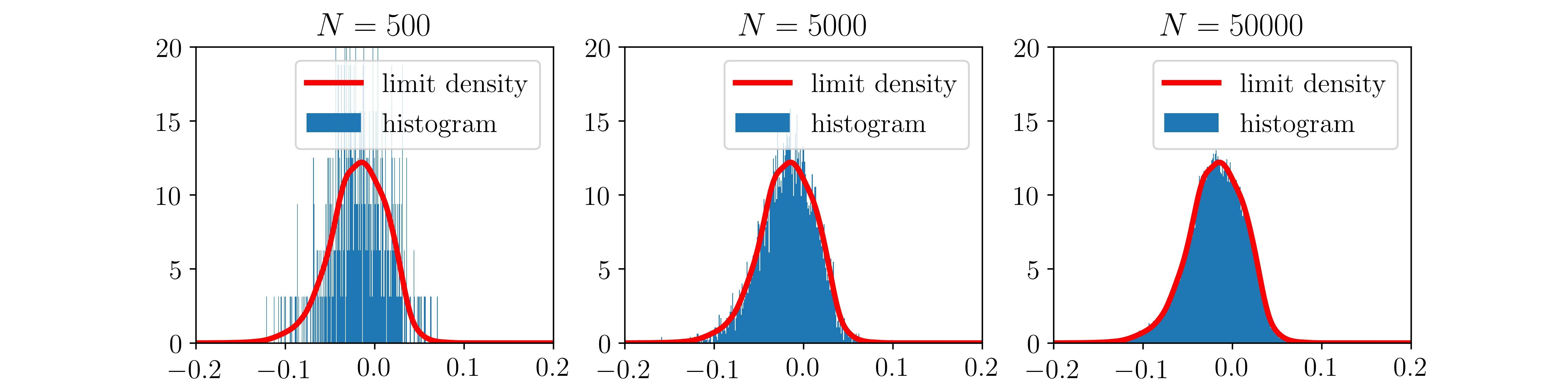
Figure 4: Convergence of the weights of the first layer as $N\to+\infty$ for $\alpha=0$ and $M=100$. The first line corresponds to $\beta=0.25$, the second to $\beta=0.5$, the third to $\beta=0.75$ and the last line to $\beta=1.0$.

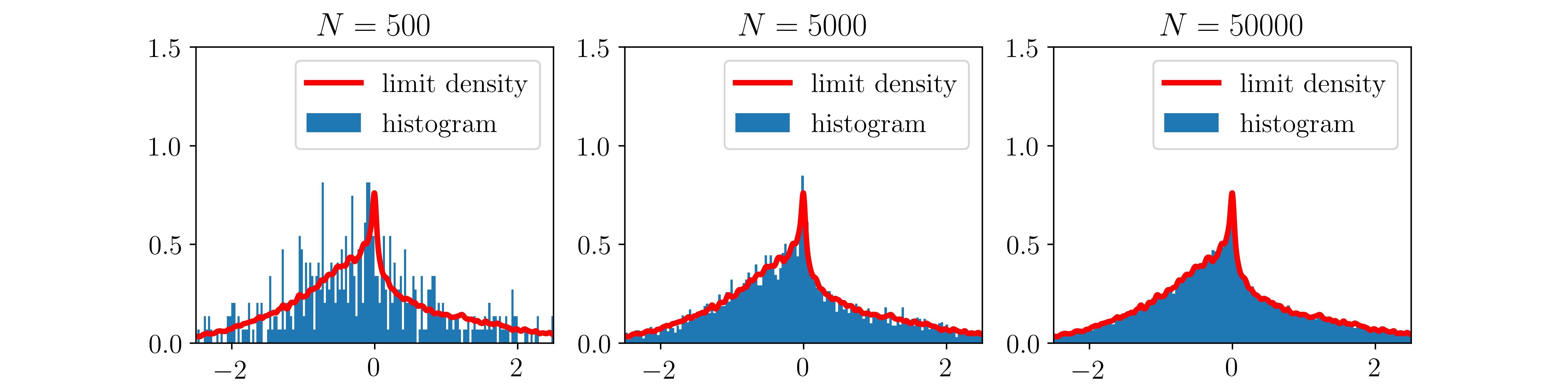
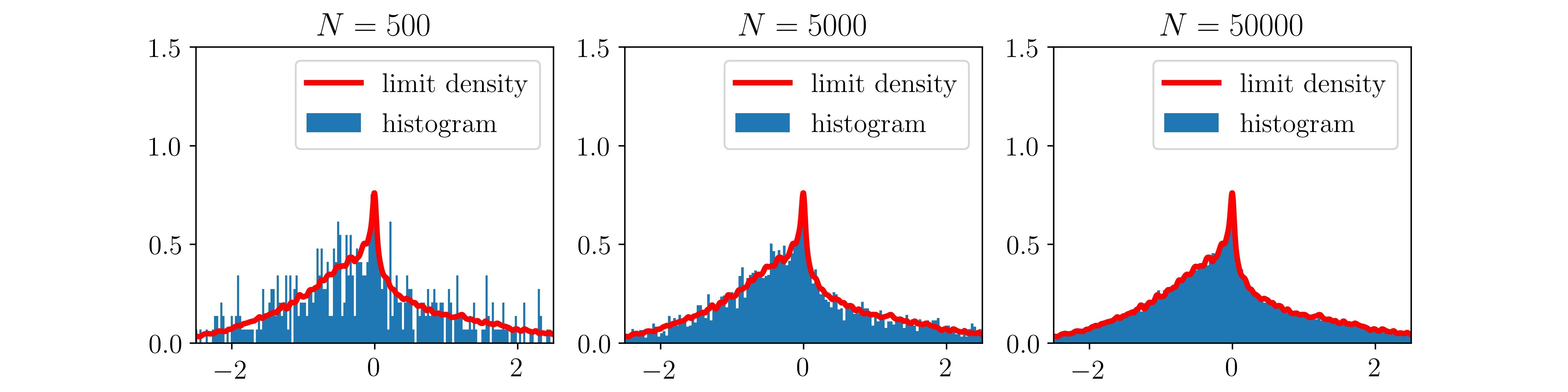
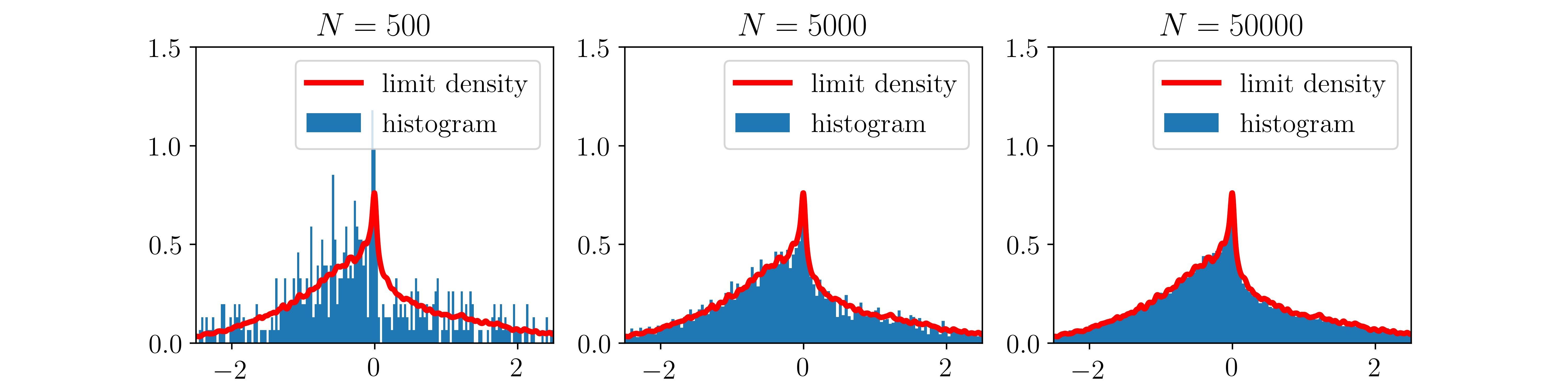
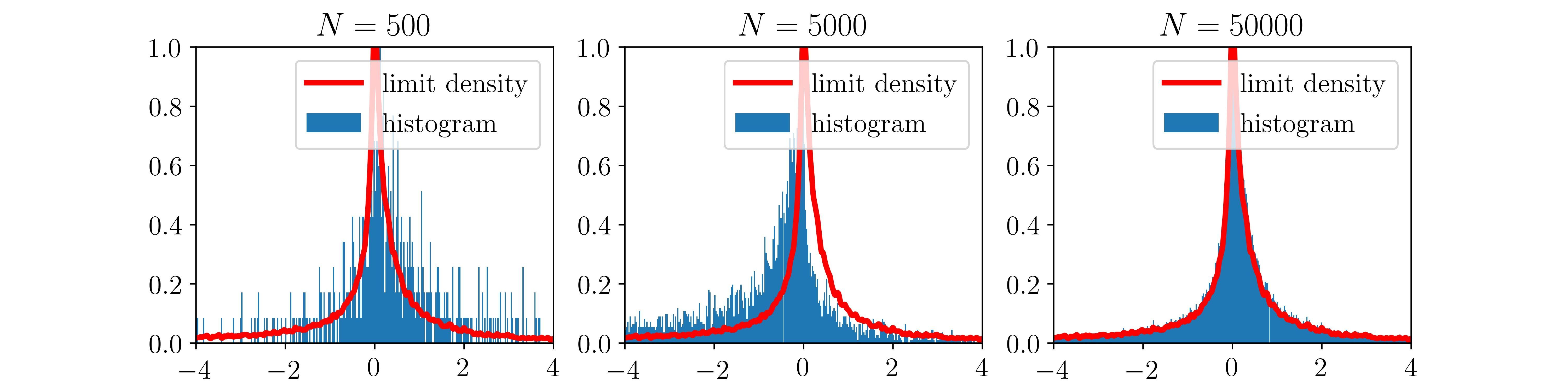
Figure 5: Convergence of the weights of the first layer as $N\to+\infty$ for $\alpha=0$ and $M=100$. The first line corresponds to $\beta=0.25$, the second to $\beta=0.5$, the third to $\beta=0.75$ and the last line to $\beta=1.0$.

On Figure 6 and Figure 7 we show the results of the exact same experiments but this time using decreasing stepsizes and a parameter $\alpha=0.25$. Once again our experiments illustrate the convergence of the empirical distributions to some limiting distribution, and we can also identify two regimes. Note that the limiting distribution satisfying (170) or (173) (depending on the value of $\beta$), it depends on the parameter $\alpha$. Therefore the limiting distribution obtained in the case where $\alpha=0.25$ is different from the one obtained when $\alpha=0$. This is particularly visible in the case where $\beta=1$ (as shown in green on Figure 6 and Figure 7).

Figure 6: Convergence of the weights of the first layer as $N\to+\infty$ for $\alpha=0.25$ and $M=100$. The first line corresponds to $\beta=0.5$, the second to $\beta=0.75$ and the last line to $\beta=1.0$.

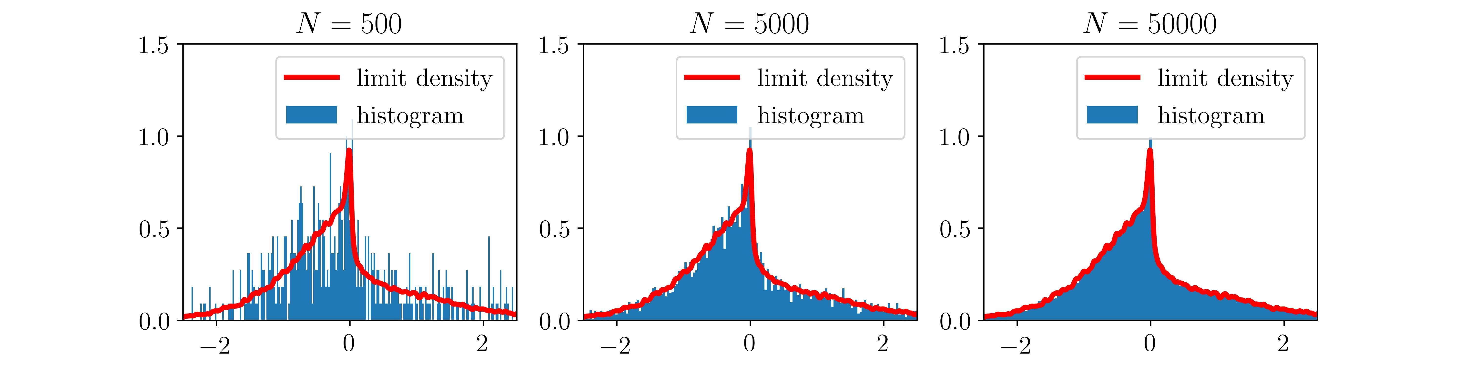
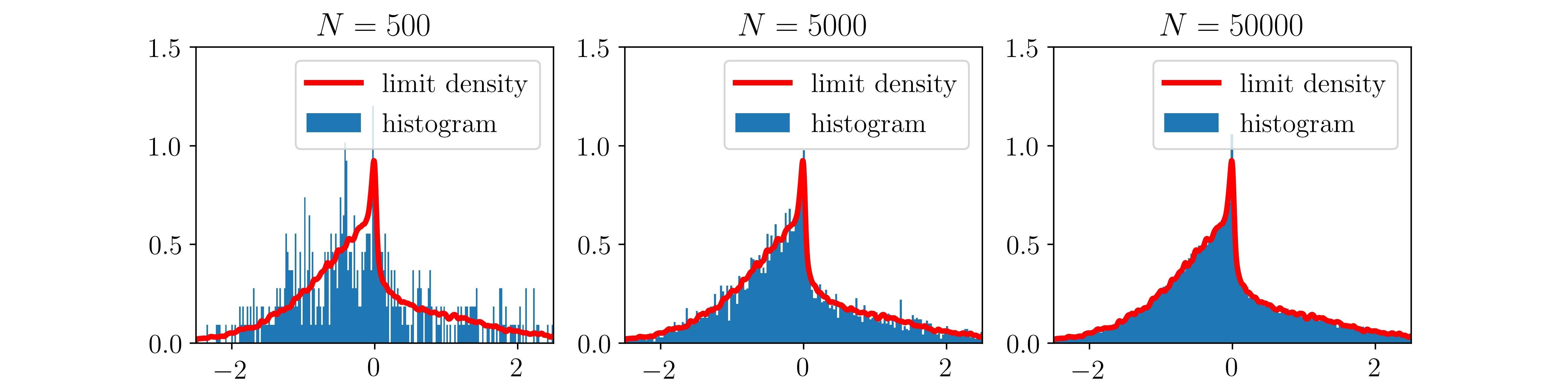
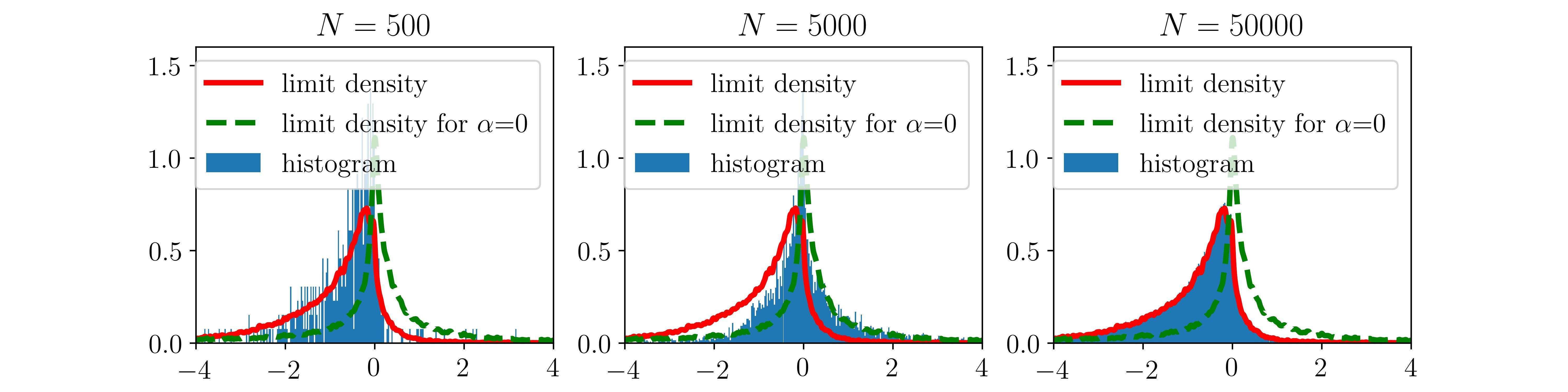
Figure 7: Convergence of the weights of the first layer as $N\to+\infty$ for $\alpha=0.25$ and $M=100$. The first line corresponds to $\beta=0.5$, the second to $\beta=0.75$ and the last line to $\beta=1.0$.

We now study the role of the batch size $M$ on the convergence toward the mean-field regime. Figure 8 illustrates the convergence of the empirical measures in the case where $\beta<1$ (here $\beta=0.75$) of the weights of the hidden layer of the neural network, for a fixed number of neurons $N=10000$ for different batch sizes $M$. We indeed observe convergence with $M$.

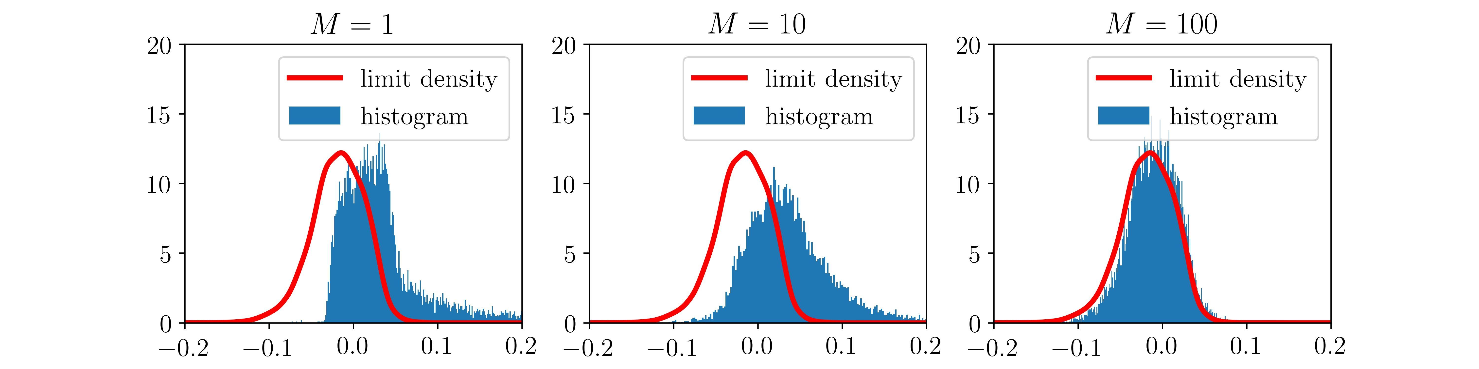
Figure 8: Convergence of the weights as $M\to\infty$

References

- [1] I. Goodfellow, Y. Bengio, and A. Courville, Deep Learning. MIT Press, 2016.
- [2] A. Krizhevsky, I. Sutskever, and G. Hinton, “Imagenet classification with deep convolutional neural networks,” in Advances in neural information processing systems, pp. 1097–1105, 2012.
- [3] C. Manning and H. Schütze, Foundations of statistical natural language processing. MIT press, 1999.
- [4] C. Zhang, S. Bengio, M. Hardt, B. Recht, and O. Vinyals, “Understanding deep learning requires rethinking generalization,” arXiv preprint arXiv:1611.03530, 2016.
- [5] S. Shalev-Shwartz and S. Ben-David, Understanding machine learning: From theory to algorithms. Cambridge university press, 2014.
- [6] H. Li, Z. Xu, G. Taylor, C. Studer, and T. Goldstein, “Visualizing the loss landscape of neural nets,” in Advances in Neural Information Processing Systems, pp. 6389–6399, 2018.
- [7] A. Ballard, R. Das, S. Martiniani, D. Mehta, L. Sagun, J. Stevenson, and D. Wales, “Energy landscapes for machine learning,” Physical Chemistry Chemical Physics, vol. 19, no. 20, pp. 12585–12603, 2017.
- [8] M. Soltanolkotabi, A. Javanmard, and J. Lee, “Theoretical insights into the optimization landscape of over-parameterized shallow neural networks,” IEEE Trans. Information Theory, vol. 65, no. 2, pp. 742–769, 2019.
- [9] K. Fukumizu and S. Amari, “Local minima and plateaus in hierarchical structures of multilayer perceptrons,” Neural networks, vol. 13, no. 3, pp. 317–327, 2000.
- [10] A. J. Bray and D. Dean, “Statistics of critical points of gaussian fields on large-dimensional spaces,” Physical review letters, vol. 98, no. 15, p. 150201, 2007.
- [11] R. Pascanu, Y. N. Dauphin, S. Ganguli, and Y. Bengio, “On the saddle point problem for non-convex optimization,” arXiv preprint arXiv:1405.4604, 2014.
- [12] J. Pennington and Y. Bahri, “Geometry of neural network loss surfaces via random matrix theory,” in Proceedings of the 34th International Conference on Machine Learning-Volume 70, pp. 2798–2806, JMLR. org, 2017.
- [13] K. Kawaguchi, “Deep learning without poor local minima,” in Advances in neural information processing systems, pp. 586–594, 2016.
- [14] D. Freeman and J. Bruna, “Topology and geometry of half-rectified network optimization,” arXiv preprint arXiv:1611.01540, 2016.
- [15] L. Venturi, A. Bandeira, and J. Bruna, “Neural networks with finite intrinsic dimension have no spurious valleys,” CoRR, vol. abs/1802.06384, 2018.
- [16] F. Bach, “Breaking the curse of dimensionality with convex neural networks,” The Journal of Machine Learning Research, vol. 18, no. 1, pp. 629–681, 2017.
- [17] A. Choromanska, M. Henaff, M. Mathieu, G. Ben Arous, and Y. LeCun, “The loss surfaces of multilayer networks,” in Artificial intelligence and statistics, pp. 192–204, 2015.
- [18] L. Venturi, A. S. Bandeira, and J. Bruna, “Spurious valleys in one-hidden-layer neural network optimization landscapes,” Journal of Machine Learning Research, vol. 20, no. 133, pp. 1–34, 2019.
- [19] R. Kuditipudi, X. Wang, H. Lee, Y. Zhang, Z. Li, W. Hu, R. Ge, and S. Arora, “Explaining landscape connectivity of low-cost solutions for multilayer nets,” in Advances in Neural Information Processing Systems 32 (H. Wallach, H. Larochelle, A. Beygelzimer, F. d’Alché Buc, E. Fox, and R. Garnett, eds.), pp. 14601–14610, Curran Associates, Inc., 2019.
- [20] Z. Allen-Zhu, Y. Li, and Z. Song, “On the convergence rate of training recurrent neural networks,” in Advances in Neural Information Processing Systems 32 (H. Wallach, H. Larochelle, A. Beygelzimer, F. d’Alché Buc, E. Fox, and R. Garnett, eds.), pp. 6676–6688, Curran Associates, Inc., 2019.
- [21] S. S. Mannelli, G. Biroli, C. Cammarota, F. Krzakala, and L. Zdeborová, “Who is afraid of big bad minima? analysis of gradient-flow in spiked matrix-tensor models,” in Advances in Neural Information Processing Systems 32 (H. Wallach, H. Larochelle, A. Beygelzimer, F. d’Alché Buc, E. Fox, and R. Garnett, eds.), pp. 8679–8689, Curran Associates, Inc., 2019.
- [22] J. Sirignano and K. Spiliopoulos, “Mean field analysis of neural networks,” arXiv preprint arXiv:1805.01053, 2018.
- [23] S. Mei, A. Montanari, and P. Nguyen, “A mean field view of the landscape of two-layer neural networks,” Proceedings of the National Academy of Sciences, vol. 115, no. 33, pp. E7665–E7671, 2018.
- [24] G. M. Rotskoff and E. Vanden-Eijnden, “Trainability and accuracy of neural networks: An interacting particle system approach,” 2018.
- [25] S. Mei, T. Misiakiewicz, and A. Montanari, “Mean-field theory of two-layers neural networks: dimension-free bounds and kernel limit,” arXiv preprint arXiv:1902.06015, 2019.
- [26] A. Javanmard, M. Mondelli, and A. Montanari, “Analysis of a two-layer neural network via displacement convexity,” arXiv preprint arXiv:1901.01375, 2019.
- [27] L. Chizat, “Sparse optimization on measures with over-parameterized gradient descent,” arXiv preprint arXiv:1907.10300, 2019.
- [28] L. Chizat and F. Bach, “On the global convergence of gradient descent for over-parameterized models using optimal transport,” in Advances in neural information processing systems, pp. 3036–3046, 2018.
- [29] J. Jabir, D. vSivska, and L. Szpruch, “Mean-field neural odes via relaxed optimal control,” arXiv preprint arXiv:1912.05475, 2019.
- [30] L. Ambrosio, N. Gigli, and G. Savaré, Gradient flows in metric spaces and in the space of probability measures. Lectures in Mathematics ETH Zürich, Birkhäuser Verlag, Basel, second ed., 2008.
- [31] M. Erbar, “The heat equation on manifolds as a gradient flow in the wasserstein space,” in Annales de l’institut Henri Poincaré (B), vol. 46, pp. 1–23, 2010.
- [32] L. Ambrosio, G. Savaré, and L. Zambotti, “Existence and stability for Fokker–Planck equations with log-concave reference measure,” Probability Theory and Related Fields, vol. 145, no. 3, pp. 517–564, 2009.
- [33] A. Sznitman, “Topics in propagation of chaos,” in Ecole d’été de probabilités de Saint-Flour XIX—1989, pp. 165–251, Springer, 1991.
- [34] A. Gottlieb, “Markov transitions and the propagation of chaos,” arXiv preprint math/0001076, 2000.
- [35] S. Méléard and S. Roelly-Coppoletta, “Systèmes de particules et mesures-martingales: un théorème de propagation du chaos,” Séminaire de probabilités de Strasbourg, vol. 22, pp. 438–448, 1988.
- [36] R. Jordan, D. Kinderlehrer, and F. Otto, “The variational formulation of the fokker–planck equation,” SIAM journal on mathematical analysis, vol. 29, no. 1, pp. 1–17, 1998.
- [37] H. P. McKean, Jr., “Propagation of chaos for a class of non-linear parabolic equations,” in Stochastic Differential Equations (Lecture Series in Differential Equations, Session 7, Catholic Univ., 1967), pp. 41–57, Air Force Office Sci. Res., Arlington, Va., 1967.
- [38] X. Fontaine, V. D. Bortoli, and A. Durmus, “Continuous and discrete-time analysis of stochastic gradient descent for convex and non-convex functions,” 2020.
- [39] M. Welling and Y. Teh, “Bayesian learning via stochastic gradient langevin dynamics,” in Proceedings of the 28th international conference on machine learning (ICML-11), pp. 681–688, 2011.
- [40] J. Sirignano and K. Spiliopoulos, “Mean field analysis of neural networks: A central limit theorem,” Stochastic Processes and their Applications, vol. 130, no. 3, pp. 1820–1852, 2020.
- [41] Y. LeCun and C. Cortes, “MNIST handwritten digit database,” 2010.
- [42] A. Krizhevsky, G. Hinton, et al., “Learning multiple layers of features from tiny images,” 2009.
- [43] C. Villani, Optimal transport, vol. 338 of Grundlehren der Mathematischen Wissenschaften [Fundamental Principles of Mathematical Sciences]. Springer-Verlag, Berlin, 2009. Old and new.
- [44] A. Kechris, Classical Descriptive Set Theory. Graduate Texts in Mathematics, Springer New York, 2012.
- [45] D. W. Stroock and S. R. S. Varadhan, Multidimensional diffusion processes. Classics in Mathematics, Springer-Verlag, Berlin, 2006. Reprint of the 1997 edition.
- [46] I. Karatzas and S. E. Shreve, Brownian motion and stochastic calculus, vol. 113 of Graduate Texts in Mathematics. Springer-Verlag, New York, second ed., 1991.
- [47] L. C. G. Rogers and D. Williams, Diffusions, Markov processes, and martingales. Vol. 2. Cambridge Mathematical Library, Cambridge University Press, Cambridge, 2000. Itô calculus, Reprint of the second (1994) edition.
- [48] Y. Nesterov, Introductory lectures on convex optimization, vol. 87 of Applied Optimization. Kluwer Academic Publishers, Boston, MA, 2004. A basic course.
- [49] L. Ambrosio and N. Gigli, “A user’s guide to optimal transport,” in Modelling and optimisation of flows on networks, vol. 2062 of Lecture Notes in Math., pp. 1–155, Springer, Heidelberg, 2013.
- [50] F. F. Bonsall and K. Vedak, Lectures on some fixed point theorems of functional analysis. No. 26, Tata Institute of Fundamental Research Bombay, 1962.
- [51] J. Kent, “Time-reversible diffusions,” Advances in Applied Probability, vol. 10, pp. 819–835, 12 1978.