Impurity Lattice Monte Carlo for Hypernuclei

Abstract

We consider the problem of including $\Lambda$ hyperons into the ab initio framework of nuclear lattice effective field theory. In order to avoid large sign oscillations in Monte Carlo simulations, we make use of the fact that the number of hyperons is typically small compared to the number of nucleons in the hypernuclei of interest. This allows us to use the impurity lattice Monte Carlo method, where the minority species of fermions in the full nuclear Hamiltonian is integrated out and treated as a worldline in Euclidean projection time. The majority fermions (nucleons) are treated as explicit degrees of freedom, with their mutual interactions described by auxiliary fields. This is the first application of the impurity lattice Monte Carlo method to systems where the majority particles are interacting. Here, we show how the impurity Monte Carlo method can be applied to compute the binding energy of the light hypernuclei. In this exploratory work we use spin-independent nucleon-nucleon and hyperon-nucleon interactions to test the computational power of the method. We find that the computational effort scales approximately linearly in the number of nucleons. The results are very promising for future studies of larger hypernuclear systems using chiral effective field theory and realistic hyperon-nucleon interactions, as well as applications to other quantum many-body systems.

1 Introduction

Hypernuclei are bound states of one or two hyperons together with a core composed of nucleons. They extend the nuclear chart into a third dimension, augmenting the usual two dimensions of proton number and neutron number. We will use the notation $Y$ for a $\Lambda$ or $\Sigma$ hyperon and $N$ for a nucleon. Due to the scarcity of direct hyperon-nucleon ($YN$) and hyperon-hyperon ($YY$) scattering data, these unusual forms of baryonic matter play an important role in pinning down the fundamental baryon-baryon forces. This requires on the one hand an effective field theory (EFT) description of the underlying forces, as pioneered in Ref. Korpa:2001au ; Polinder:2006zh , and on the other hand a numerically precise and consistent method to solve the nuclear $A$-body problem, such as nuclear lattice EFT (NLEFT) Lee:2008fa ; Lahde:2019npb . For calculations combining these chiral EFT forces at LO and NLO Haidenbauer:2013oca ; Haidenbauer:2019boi with other many-body methods, see e.g. Ref. Lonardoni:2013rm ; Gazda:2016qva ; Wirth:2017lso ; Wirth:2017bpw ; Le:2019gjp ; Haidenbauer:2019thx .

In view of the success of NLEFT in the description of nuclear spectra and reactions, it seems natural to extend this method to hypernuclei. However, this is not quite straightforward. While one can extend the four spin-isospin degrees of freedom comprising the nucleons to include the $\Lambda$ and $\Sigma$ states Bour , this has not been done because there is no longer an approximate symmetry such as Wigner’s SU(4) symmetry Wigner:1936dx that protects the Monte Carlo (MC) simulations against strong sign oscillations when using auxiliary fields. The physics of hypernuclei therefore requires a different approach, and in this paper we show how the computational problems are solved using the impurity lattice Monte Carlo (ILMC) method.

The ILMC method was introduced in Ref. Elhatisari:2014lka in the context of a Hamiltonian theory of spin-up and spin-down fermions, and applied to the intrinsically non-perturbative physics of Fermi polarons in two dimensions in Ref. Bour:2014bxa . The ILMC method is particularly useful for the case where only one fermion (of either species) is immersed in a “sea” of the other species. Within the standard auxiliary field Monte Carlo method, such an extreme imbalance would lead to unacceptable sign oscillations in the Monte Carlo probability weight. In the ILMC method, the minority particle is “integrated out”, resulting in a formalism where only the majority species fermions appear as explicit degrees of freedom, while the minority fermion is represented by a “worldline” in Euclidean projection time. The spatial position of this worldline is updated using Monte Carlo updates, while the interactions between the majority fermions are described by the auxiliary field formalism Lahde:2019npb .

Here, we apply the ILMC method to the inclusion of hyperons into NLEFT simulations. We identify the $\Lambda$ hyperon as the minority species, which we represent by a worldline in Euclidean time. This $\Lambda$ worldline is treated as immersed in an environment consisting of some number of nucleons. We focus on the Monte Carlo calculation of the binding energy of light hypernuclei, by means of a simplified $YN$ interaction, consisting of a single contact interaction, tuned to a best description of the the empirical binding energies of the $s$-shell hypernuclei with $A=3,4,5$. For the $NN$ interaction, we use a simple leading order interaction similar to that described in Ref. Lu:2018bat . We benchmark our ILMC results against Lanczos calculations of transfer matrix and exact Euclidean projection calculations with initial/final states and number of time steps that match the ILMC calculations. We note that our Monte Carlo method is free from any approximation about the nodal structure of the many-body wave function. This is the first application of such unconstrained Monte Carlo simulations to hypernuclei.

This paper is organized as follows. In Sec. 2, we present the path integral formalism for our system of nucleons and one hyperon. We first write the nucleon-nucleon interaction first without auxiliary fields and then with auxiliary fields. In Sec. 3 we present the equivalent system using normal-ordered transfer matrices. In Sec. 4, we derive the impurity worldline formalism for the chosen $YN$ interaction, and introduce the concept of the “reduced” transfer matrix operator, which acts on the nucleons only. In Sec. 5, we discuss the Monte Carlo updating of the hyperon worldline and the auxiliary fields, which encode the interactions between nucleons. In Sec. 6, we present results for the ground state energies of the $s$-shell nuclei and hypernuclei. In Sec. 7, we conclude with a discussion of future improvements and applications of the impurity lattice Monte Carlo method to hypernuclei and other quantum many-body systems.

2 Path integral formalism

We develop the ILMC formalism following Ref. Elhatisari:2014lka , who considered a system of spin-up and spin-down fermions, with a contact interaction which operates between fermions of opposite spin. The situation here is completely analogous, we have one majority species, the nucleons, and one impurity, the $\Lambda$. As usual in NLEFT, we consider positions on a spatial lattice denoted by $\vec{n}$ and lattice spacing $a$. We also assume that Euclidean time has been discretized, such that slices of the Euclidean time are denoted by $n_{t}$ with temporal lattice spacing $a_{t}$. The partition function can be expressed in terms of the Grassmann path integral

$$\mathcal{Z}=\int\Bigg{[}\prod_{\begin{subarray}{c}\vec{n},n_{t}\\ s=N,Y\end{subarray}}d\zeta_{s}(\vec{n},n_{t})d\zeta_{s}^{*}(\vec{n},n_{t})\Bigg{]}\exp(-S[\zeta,\zeta^{*}]),$$ (1)

where the subscripts $N$ refer to all nucleon spin and isospin components and $Y$ refers to all hyperon spin components. In this study we consider only $\Lambda$ hyperons. In future work we will also consider $\Sigma$ hyperons or account for their influence via three-baryon interactions involving a $\Lambda$ and two nucleons. We also make the simplifying assumption that the hyperon-nucleon and nucleon-nucleon interaction are spin-independent and neglect Coulomb interactions. Because of the spin-independent interaction and the fact that we have only one Lambda hyperon, from this point onward we can restrict our attention to only one spin component of the hyperon.

Assuming that the exponent of the Euclidean action in Eq. (1) is treated by a Trotter decomposition, we find

$$S[\zeta,\zeta^{*}]\equiv\sum_{n_{t}}\bigg{\{}S_{t}[\zeta,\zeta^{*},n_{t}]+S_{Y}[\zeta,\zeta^{*},n_{t}]$$

$$\quad+S_{N}[\zeta,\zeta^{*},n_{t}]+S_{YN}[\zeta,\zeta^{*},n_{t}]+S_{NN}[\zeta,\zeta^{*},n_{t}]\bigg{\}},$$ (2)

where the component due to the time derivative is

$$S_{t}[\zeta,\zeta^{*},n_{t}] \equiv\!\!\!\sum_{\vec{n},s=N,Y}\zeta_{s}^{*}(\vec{n},n_{t})$$

$$\quad\times\bigg{[}\zeta_{s}(\vec{n},n_{t}+1)-\zeta_{s}(\vec{n},n_{t})\bigg{]},$$ (3)

while $S_{Y}$ and $S_{N}$ describe the kinetic energies of the hyperons and nucleons, respectively. Further, $S_{YN}$ provides the $YN$ interaction, and $S_{NN}$ the $NN$ interaction, which we shall consider next.

2.1 The hyperon-nucleon interaction

For the hyperons, we take for simplicity the lowest-order (unimproved) kinetic energy

$$S_{Y}[\zeta,\zeta^{*},n_{t}]\equiv 6h\sum_{\vec{n}}\zeta_{Y}^{*}(\vec{n},n_{t})\zeta_{Y}(\vec{n},n_{t})$$

$$-h\sum_{\vec{n}}\sum_{l=1}^{3}\>\zeta_{Y}^{*}(\vec{n},n_{t})\bigg{[}\zeta_{Y}(\vec{n}+\hat{e}_{l},n_{t})+\zeta_{Y}(\vec{n}-\hat{e}_{l},n_{t})\bigg{]},$$ (4)

with

$$h\equiv\frac{\alpha_{t}}{2m_{Y}},$$ (5)

where $m_{Y}$ is the hyperon mass, and we have defined $\alpha_{t}\equiv a_{t}/a$ as the ratio of temporal and spatial lattice spacings.

The $YN$ interaction is given by

$$S_{YN}[\zeta,\zeta^{*},n_{t}]\equiv\alpha_{t}C_{YN}\sum_{\vec{n}}\rho_{N}(\vec{n},n_{t})\rho_{Y}(\vec{n},n_{t}),$$ (6)

where

$$\rho_{N}(\vec{n},n_{t})\equiv\sum_{i,j}\rho_{i,j}(\vec{n},n_{t})\equiv\sum_{i,j}\zeta^{*}_{i,j}(\vec{n},n_{t})\zeta_{i,j}(\vec{n},n_{t}),$$ (7)

and

$$\rho_{Y}(\vec{n},n_{t})\equiv\zeta_{Y}^{*}(\vec{n},n_{t})\zeta_{Y}(\vec{n},n_{t}),$$ (8)

are nucleon and hyperon densities, respectively, with spin $i=0,1$ (up, down) and isospin $j=0,1$ (proton, neutron). The tuning of the coupling constant $C_{YN}$ is discussed in Section 6.

Note that this is a simplified version of the pionless EFT calculation of Ref. Hammer:2001ng , which also included a three-body interaction at LO. Such an interaction is sub-leading in chiral EFT approaches (such as NLEFT). See also the recent work in Ref. Contessi:2018qnz .

2.2 The nucleon-nucleon interaction

For the kinetic energy of the nucleon degrees of freedom, we likewise use the lowest-order expression

$$S_{N}[\zeta,\zeta^{*},n_{t}]\equiv\frac{3\alpha_{t}}{m_{N}}\sum_{\vec{n}}\rho_{N}(\vec{n},n_{t})$$

$$-\frac{\alpha_{t}}{2m_{N}}\sum_{\vec{n}}\sum_{l=1}^{3}\left[\rho_{N}(\vec{n},\vec{n}+\hat{e}_{l},n_{t})+\rho_{N}(\vec{n},\vec{n}-\hat{e}_{l},n_{t})\right],$$ (9)

where

$$\rho_{N}(\vec{n},\vec{n}^{\prime},n_{t}) \equiv\sum_{i,j}\zeta^{*}_{i,j}(\vec{n},n_{t})\zeta_{i,j}(\vec{n}^{\prime},n_{t}),$$ (10)

$$\rho_{N}(\vec{n},n_{t}) \equiv\rho_{N}(\vec{n},\vec{n},n_{t}),$$ (11)

and $m_{N}$ is the nucleon mass. Here, the $\hat{e}_{l}$ are unit vectors in lattice direction $l$.

The Wigner SU(4)-symmetric part of the leading-order (LO) $NN$ interaction of Refs. Elhatisari:2016owd ; Elhatisari:2017eno ; Li:2018ymw is used for the present work. This is an approximate symmetry Wigner:1936dx of the low-energy nucleon-nucleon interactions, where the spin and isospin degrees of freedom of the nucleons can be rotated as four components of an SU(4) multiplet. We have

$$S_{NN}[\zeta,\zeta^{*},n_{t}] \equiv\frac{\alpha_{t}C_{NN}}{2}\!\!\!\sum_{\vec{n},\vec{n}^{\prime},\vec{n}^{\prime\prime}}\rho_{N}^{s}(\vec{n}^{\prime},n_{t})f_{s_{\rm L}}(\vec{n}^{\prime}-\vec{n})$$

$$\quad\times f_{s_{\rm L}}(\vec{n}-\vec{n}^{\prime\prime})\rho_{N}^{s}(\vec{n}^{\prime\prime},n_{t}),$$ (12)

where

$$\rho_{N}^{s}(\vec{n},n_{t})\equiv\sum_{i,j}\zeta^{s_{\rm NL}*}_{i,j}(\vec{n},n_{t})\zeta^{s_{\rm NL}}_{i,j}(\vec{n},n_{t}),$$ (13)

is the smeared nucleon density, and the (local) smearing function $f_{s_{\rm L}}$ is defined as

$$f_{s_{\rm L}}(\vec{n}) \equiv 1\;{\rm for}\;|\vec{n}|=0,$$

$$\equiv s_{\rm L}\;{\rm for}\;|\vec{n}|=1,$$

$$\equiv 0\;{\rm otherwise},$$ (14)

and the (non-locally) smeared Grassmann fields are given by

$$\zeta^{s_{\rm NL}}_{i,j}(\vec{n},n_{t})\equiv\zeta_{i,j}(\vec{n},n_{t})+s_{\rm NL}\sum_{|\vec{n}^{\prime}|=1}\zeta_{i,j}(\vec{n}+\vec{n}^{\prime},n_{t}),$$ (15)

and

$$\zeta^{s_{\rm NL}*}_{i,j}(\vec{n},n_{t})\equiv\zeta^{*}_{i,j}(\vec{n},n_{t})+s_{\rm NL}\sum_{|\vec{n}^{\prime}|=1}\zeta^{*}_{i,j}(\vec{n}+\vec{n}^{\prime},n_{t}),$$ (16)

where the values of the parameters $C_{NN}$, $s_{\rm L}$ and $s_{\rm NL}$ used for the present work are discussed in Section 6 (see also Ref. Lu:2018bat for a full treatment).

For the $NN$ interaction we can reduce the expressions quadratic in the nucleon densities using the relation

$$\exp\left(-\frac{\alpha_{t}C_{NN}}{2}\tilde{\rho}^{2}\right)=$$

$$\frac{1}{\sqrt{2\pi}}\int_{-\infty}^{\infty}d\phi\,e^{-\frac{\phi^{2}}{2}}\exp\left(\sqrt{-\alpha_{t}C_{NN}}\,\phi\tilde{\rho}\right),$$ (17)

where

$$\tilde{\rho}\equiv\sum_{\vec{n}^{\prime}}f_{s_{\rm L}}(\vec{n}-\vec{n}^{\prime})\rho_{N}^{s}(\vec{n}^{\prime},n_{t}),$$ (18)

for each lattice site ($\vec{n},n_{t}$), such that $\phi(\vec{n},n_{t})$ is treated as a scalar auxiliary (Hubbard-Stratonovich) field. The $NN$ action then becomes

$$\exp(-S_{NN}[\zeta,\zeta^{*},n_{t}])$$

$$=\int\prod_{\vec{n}}\left[\frac{d\phi(\vec{n},n_{t})}{\sqrt{2\pi}}e^{-\frac{1}{2}\phi^{2}(\vec{n},n_{t})}\right]\exp(-S_{\phi N}[\zeta,\zeta^{*},n_{t}]),$$ (19)

for Euclidean time slice $n_{t}$, where

$$S_{\phi N}[\zeta,\zeta^{*},n_{t}]=-\sqrt{-\alpha_{t}C_{NN}}$$

$$\qquad\times\sum_{\vec{n},\vec{n}^{\prime}}\phi(\vec{n},n_{t})f_{s_{\rm L}}(\vec{n}-\vec{n}^{\prime})\rho_{N}^{s}(\vec{n}^{\prime},n_{t}),$$ (20)

for $C_{NN}<0$.

In the ILMC calculations, the path integral over the auxiliary field $\phi$ is evaluated using either local Metropolis algorithm updates or global lattice updates using the hybrid Monte Carlo (HMC) algorithm. See Ref. Lu:2018bat for more details on efficient Monte Carlo algorithms.

3 Transfer matrix formalism

Derivations of Feynman rules are usually easier to perform in the Grassmann formalism. However, actual NLEFT calculations are performed using the transfer matrix Monte Carlo method. As noted in Ref. Elhatisari:2014lka , the Grassmann and transfer matrix operator formulations are connected by the exact relationship

$$\mathrm{Tr}\big{\{}:f_{N_{t}-1}[a_{s}(\vec{n}),a_{s^{\prime}}^{\dagger}(\vec{n}^{\prime})]:\cdots:f_{0}[a_{s}(\vec{n}),a_{s^{\prime}}^{\dagger}(\vec{n}^{\prime})]:\big{\}}=$$

$$\int\Bigg{[}\prod_{\begin{subarray}{c}\vec{n},n_{t}\\ s=N,Y\end{subarray}}d\zeta_{s}(\vec{n},n_{t})d\zeta_{s}^{*}(\vec{n},n_{t})\Bigg{]}\exp\left(-\sum_{n_{t}}S_{t}[\zeta,\zeta^{*},n_{t}]\right)$$

$$\quad\times\prod_{n_{t}=0}^{N_{t}-1}f_{n_{t}}\big{[}\zeta_{s}(\vec{n},n_{t}),\zeta_{s^{\prime}}^{*}(\vec{n}^{\prime},n_{t})\big{]},$$ (21)

where $f$ is an arbitrary function, $a_{s}^{\dagger}$ and $a_{s}$ denote creation and annihilation operators for the fermion degrees of freedom, and the colons signify normal ordering. Using this identity, we can write the partition function in Eq. (1) as

$$\mathcal{Z}=\mathrm{Tr}(\hat{M}^{N_{t}}),$$ (22)

where $\hat{M}$ is the (normal-ordered) transfer matrix operator.

We can use Eq. (21) to define the full transfer matrix operator as

$$\hat{M}=\,:\exp(-\alpha_{t}\hat{H}):.$$ (23)

with Hamiltonian

$$\hat{H}\equiv\hat{H}_{0}^{N}+\hat{H}_{0}^{Y}+\hat{H}_{NN}+\hat{H}_{YN}.$$ (24)

We now go through each of these terms. The nucleon kinetic energy term is

$$\hat{H}_{0}^{N} \equiv\frac{3}{m_{N}}\sum_{\vec{n}}\hat{\rho}_{N}(\vec{n})$$

$$-\frac{1}{2m_{N}}\sum_{\vec{n}}\sum_{l=1}^{3}\left[\hat{\rho}_{N}(\vec{n},\vec{n}+\hat{e}_{l})+\hat{\rho}_{N}(\vec{n},\vec{n}-\hat{e}_{l})\right],$$ (25)

with

$$\hat{\rho}_{N}(\vec{n},\vec{n}^{\prime}) \equiv\sum_{i,j}a^{\dagger}_{i,j}(\vec{n})a_{i,j}(\vec{n}^{\prime}),$$ (26)

$$\hat{\rho}_{N}(\vec{n}) \equiv\hat{\rho}_{N}(\vec{n},\vec{n}).$$ (27)

The hyperon kinetic energy term is

$$\hat{H}_{0}^{N} \equiv\frac{3}{m_{Y}}\sum_{\vec{n}}\hat{\rho}_{Y}(\vec{n})$$

$$-\frac{1}{2m_{Y}}\sum_{\vec{n}}\sum_{l=1}^{3}\left[\hat{\rho}_{Y}(\vec{n},\vec{n}+\hat{e}_{l})+\hat{\rho}_{Y}(\vec{n},\vec{n}-\hat{e}_{l})\right],$$ (28)

with

$$\hat{\rho}_{Y}(\vec{n},\vec{n}^{\prime}) \equiv\sum_{i,j}a^{\dagger}_{Y}(\vec{n})a_{Y}(\vec{n}^{\prime}),$$ (29)

$$\hat{\rho}_{Y}(\vec{n}) \equiv\hat{\rho}_{Y}(\vec{n},\vec{n}).$$ (30)

The $NN$ interaction is

$$\hat{H}_{NN} =\frac{C_{NN}}{2}:\!\!\!\sum_{\vec{n},\vec{n}^{\prime},\vec{n}^{\prime\prime}}\hat{\rho}_{N}^{s}(\vec{n}^{\prime})f_{s_{\rm L}}(\vec{n}^{\prime}-\vec{n})$$

$$\quad\times f_{s_{\rm L}}(\vec{n}-\vec{n}^{\prime\prime})\hat{\rho}_{N}^{s}(\vec{n}^{\prime\prime}):,$$ (31)

with

$$\hat{\rho}_{N}^{s}(\vec{n})\equiv\sum_{i,j}a^{s_{\rm NL}\dagger}_{i,j}(\vec{n})a^{s_{\rm NL}}_{i,j}(\vec{n}),$$ (32)

and the operators $a^{s_{\rm NL}\dagger}_{i,j}(\vec{n})$ and $a^{s_{\rm NL}}_{i,j}(\vec{n})$ are defined in terms of the (non-locally) smeared annihilation and creation operators

$$a^{s_{\rm NL}}_{i,j}(\vec{n})\equiv a_{i,j}(\vec{n})+s_{\rm NL}\sum_{|\vec{n}^{\prime}|=1}a_{i,j}(\vec{n}+\vec{n}^{\prime}),$$ (33)

and

$$a^{s_{\rm NL}\dagger}_{i,j}(\vec{n})\equiv a^{\dagger}_{i,j}(\vec{n})+s_{\rm NL}\sum_{|\vec{n}^{\prime}|=1}a^{\dagger}_{i,j}(\vec{n}+\vec{n}^{\prime}).$$ (34)

The $YN$ interaction is

$$\hat{H}_{YN}=C_{YN}\sum_{\vec{n}}\hat{\rho}_{N}(\vec{n})\hat{\rho}_{Y}(\vec{n}).$$ (35)

When rewriting the nucleon-nulceon interaction with auxiliary fields, the partition function takes the form

$$\mathcal{Z}=\int \prod_{\vec{n},n_{t}}\left[\frac{d\phi(\vec{n},n_{t})}{\sqrt{2\pi}}e^{-\frac{1}{2}\phi^{2}(\vec{n},n_{t})}\right]\mathrm{Tr}[\hat{M}^{(N_{t}-1)}\cdots\hat{M}^{(0)}],$$ (36)

where

$$\hat{M}^{(n_{t})}\equiv\,:\exp(-\alpha_{t}\hat{H}^{(n_{t})}):,$$ (37)

with

$$\hat{H}^{(n_{t})}\equiv\hat{H}_{0}^{N}+\hat{H}_{0}^{Y}+\hat{H}^{(n_{t})}_{\phi N}+\hat{H}_{YN},$$ (38)

and

$$\hat{H}^{(n_{t})}_{\phi N}=-\sqrt{-\alpha_{t}C_{NN}}$$

$$\qquad\times\sum_{\vec{n},\vec{n}^{\prime}}\phi(\vec{n},n_{t})f_{s_{\rm L}}(\vec{n}-\vec{n}^{\prime})\hat{\rho}_{N}^{s}(\vec{n}^{\prime},n_{t}).$$ (39)

4 Impurity worldlines and reduced transfer matrices

We now integrate out the hyperon degree of freedom and derive a “reduced” transfer matrix operator $\hat{\not{M}}$, which acts on the nucleon degrees of freedom only. Let us consider the transfer matrix between time slices $n_{t}$ and $n_{t}+1$. Let $\ket{\vec{n}}$ represent the state with the hyperon at lattice site $\vec{n}$. We first consider the case when the hyperon hops from lattice site $\vec{n}$ to $\vec{n}\pm\hat{e}_{l}$. We then have

$$\braket{\vec{n}\pm\hat{e}_{l}}{\hat{M}^{(n_{t})}}{\vec{n}}={\hat{\not{M}}}^{(n_{t})}_{\vec{n}\pm\hat{e}_{l},\vec{n}}$$ (40)

where ${\hat{\not{M}}}^{(n_{t})}_{\vec{n}\pm\hat{e}_{l},\vec{n}}$ is the reduced transfer matrix operator acting on only the nucleons with

$$\hat{\not{M}}^{(n_{t})}_{\vec{n}\pm\hat{e}_{l},\vec{n}}=h:\exp(-\alpha_{t}{\hat{H}}^{(n_{t})}_{\vec{n}\pm\hat{e}_{l},\vec{n}}):,$$ (41)

where

$${\hat{H}}^{(n_{t})}_{\vec{n}\pm\hat{e}_{l},\vec{n}}=H_{0}^{N}+\hat{H}_{0}^{Y}+\hat{H}^{(n_{t})}_{\phi N}.$$ (42)

Next we consider the case when the hyperon remains at lattice site $\vec{n}$ between time slices $n_{t}$ and $n_{t}+1$. We then have

$$\braket{\vec{n}}{\hat{M}^{(n_{t})}}{\vec{n}}={\hat{\not{M}}}^{(n_{t})}_{\vec{n},\vec{n}},$$ (43)

where the reduced transfer matrix is

$$\hat{\not{M}}^{(n_{t})}_{\vec{n},\vec{n}}=(1-6h):\exp(-\alpha_{t}{\hat{H}}^{(n_{t})}_{\vec{n},\vec{n}}):,$$ (44)

with

$${\hat{H}}^{(n_{t})}_{\vec{n},\vec{n}}=H_{0}^{N}+\hat{H}_{0}^{Y}+\hat{H}^{(n_{t})}_{\phi N}+\frac{C_{YN}}{1-6h}\hat{\rho}_{N}(\vec{n})+\cdots.$$ (45)

The ellipses refers to terms with higher powers of $\hat{\rho}$ and additional factors of $\alpha_{t}$. These are lattice artifacts that disappear in the limit $\alpha_{t}\rightarrow 0$. They are needed to cancel the higher-order powers of the $C_{YN}$ term when expanding the exponential in Eq. (44) beyond the linear term. In the full transfer matrix such terms vanish upon normal ordering of the hyperon field since we have only one hyperon in our system. However, when we integrate out the hyperon worldline, such terms no longer vanish since the hyperon is no longer a dynamical field.

In our simulations here we drop all such higher-order terms from our ILMC simulations. This choice constitutes a redefinition of our starting interaction to include some small higher-body interactions between the hyperon and more than one nucleon. Since we will take $\alpha_{t}$ to be very small, the most important induced higher-body interaction is a small three-body interaction. The three-body interaction has the form

$$\hat{H}_{YNN}=-\frac{\alpha_{t}C_{YN}^{2}}{2(1-6h)}\sum_{\vec{n}}\hat{\rho}_{N}(\vec{n})\hat{\rho}_{N}(\vec{n})\hat{\rho}_{Y}(\vec{n}),$$ (46)

We see explicitly that this term is a lattice artifact that disappears when $\alpha_{t}\to 0$.

5 Monte Carlo calculation

We now describe how ILMC calculations are performed using the Projection Monte Carlo (PMC) method. Let us first assume that the impurity has been fixed at a given spatial lattice site, and that no “hopping” of the impurity occurs during the Euclidean time evolution. We shall then relax this constraint, and discuss a practical algorithm for updating the configuration of the hyperon worldline.

5.1 Stationary impurity

For a stationary hyperon impurity, the reduced transfer matrix is given by Eq. (44), and for the purposes of the PMC calculation, we define the Euclidean projection amplitude

$$Z_{jk}(N_{t})\equiv\langle\psi_{j}|\hat{\not{M}}^{N_{t}}|\psi_{k}\rangle,$$ (47)

for a product of $N_{t}$ Euclidean time slices, where $j$ and $k$ denote different initial cluster states. As usual, this is expressed as a determinant of single-particle amplitudes, which gives

$$Z_{jk}(N_{t})=\mathrm{det}\,M_{p\times p}^{jk},$$ (48)

where

$$M_{p\times p}^{jk}=\left(\begin{array}[]{c c c}\vspace{.1cm}\langle\phi_{0,j}|\hat{\not{M}}^{N_{t}}|\phi_{0,k}\rangle&\langle\phi_{0,j}|\hat{\not{M}}^{N_{t}}|\phi_{1,k}\rangle&\cdots\\ \vspace{.1cm}\langle\phi_{1,j}|\hat{\not{M}}^{N_{t}}|\phi_{0,k}\rangle&\langle\phi_{1,j}|\hat{\not{M}}^{N_{t}}|\phi_{1,k}\rangle&\cdots\\ \vdots&\vdots&\ddots\end{array}\right),$$ (49)

for $p$ nucleons. By means of the projection amplitudes (48), we construct

$$[\hat{M}^{a}(N_{t})]_{qq^{\prime}}\equiv\sum_{q^{\prime\prime}}Z_{qq^{\prime\prime}}^{-1}(N_{t})Z_{q^{\prime\prime}q^{\prime}}(N_{t}+1),$$ (50)

which is known as the “adiabatic transfer matrix”. If we denote the eigenvalues of (50) by $\lambda_{i}(N_{t})$, we find

$$\lambda_{i}(N_{t})=\exp(-\alpha_{t}E_{i}(N_{t}+1/2)),$$ (51)

such that the low-energy spectrum is given by the “transient” energies

$$E_{i}(N_{t}+1/2)=-\frac{\log(\lambda_{i}(N_{t}))}{\alpha_{t}},$$ (52)

at finite temporal lattice spacing $a_{t}$. For the case of a single trial cluster state with $p$ nucleons, Eq. (48) reduces to

$$Z(N_{t})=\mathrm{det}\,M_{p\times p}^{00},$$ (53)

for the case of a single trial state. The ground-state energy is obtained from

$$E_{0}(N_{t}+1/2)=-\frac{\log(Z(N_{t}+1)/Z(N_{t}))}{\alpha_{t}},$$ (54)

in the limit $N_{t}\to\infty$, where the exact low-energy spectrum of the transfer matrix will be recovered. Note that the argument $N_{t}+1/2$ is conventionally assigned to the transient energy computed from the ratio of projection amplitudes evaluated at Euclidean time steps $N_{t}+1$ and $N_{t}$.

As an example, for the hypertriton we have $p=2$ nucleons after the impurity hyperon has been integrated out. We start the Euclidean time projection with a single initial trial cluster state ($j=k=0$) consisting of a spin-up proton and a spin-up neutron. As there are no terms that mix spin or isospin, the other components of each single-particle state are set to zero, and remain so during the PMC calculation. For the spatial parts of the nucleon wave functions, we may choose, for example, the zero-momentum state

$$|\phi_{0,0}\rangle=|\phi_{1,0}\rangle=\langle 0,0,0\rangle,$$ (55)

in the notation of Ref. Elhatisari:2014lka , which denotes plane-wave orbitals in a cubic box. In principle, we may also choose any other plane-wave state with non-zero momentum (see Table 1 of Ref. Elhatisari:2014lka ), or any other more complicated trial state. For the heavier nuclei, it is indeed better to choose an initial state where the nucleons are clustered together. In this case we sum over all possible translations of the cluster in order construct an initial state with zero total momentum.

5.2 Hopping impurity

If the hyperon impurity is allowed to hop between nearest-neighbor sites (from one Euclidean time slice to the next), the Euclidean projection amplitude becomes a sum over hyperon worldline configurations. This gives

$$Z_{jk}(N_{t})\equiv\sum_{\vec{n}_{0},\ldots,\vec{n}_{N_{t}}}\langle\psi_{j}|\hat{\not{M}}^{N_{t}}_{\{\vec{n}_{j}\}}|\psi_{k}\rangle,$$ (56)

where the product

$$\hat{\not{M}}^{N_{t}}_{\{\vec{n}_{j}\}}\equiv\hat{\not{M}}_{\vec{n}_{N_{t}},\vec{n}_{N_{t}-1}}\hat{\not{M}}_{\vec{n}_{N_{t}-1},\vec{n}_{N_{t}-2}}\ldots\hat{\not{M}}_{\vec{n}_{2},\vec{n}_{1}}\hat{\not{M}}_{\vec{n}_{1},\vec{n}_{0}},$$ (57)

is expressed in terms of the reduced transfer matrices (44) and (41). Here, $\vec{n}_{j}$ denotes the spatial position of the hyperon impurity (which has been integrated out) on time slice $j$. The expressions for the projection amplitude and determinant are generalized to

$$Z_{jk}(N_{t})=\sum_{\vec{n}_{0},\ldots,\vec{n}_{N_{t}}}\mathrm{det}\,M_{p\times p}^{jk},$$ (58)

where

$$M_{p\times p}^{jk}=\left(\begin{array}[]{c c c}\vspace{.1cm}\langle\phi_{0,j}|\hat{\not{M}}^{N_{t}}_{\{\vec{n}_{j}\}}|\phi_{0,k}\rangle&\langle\phi_{0,j}|\hat{\not{M}}^{N_{t}}_{\{\vec{n}_{j}\}}|\phi_{1,k}\rangle&\cdots\\ \vspace{.1cm}\langle\phi_{1,j}|\hat{\not{M}}^{N_{t}}_{\{\vec{n}_{j}\}}|\phi_{0,k}\rangle&\langle\phi_{1,j}|\hat{\not{M}}^{N_{t}}_{\{\vec{n}_{j}\}}|\phi_{1,k}\rangle&\cdots\\ \vdots&\vdots&\ddots\end{array}\right),$$ (59)

such that the determinant is now to be computed over all possible hyperon wordline configurations.

We note that the worldline configuration is to be updated stochastically using a Metropolis algorithm. Thus, proposed changes in the impurity worldline are accepted or rejected by importance sampling with $|Z_{jj}(N_{t})|$ as the probability weight function. Here, $j$ denotes one of the initial trial nucleon cluster states.

5.3 Worldline updates

The updating of the impurity worldline is handled in two steps: The generation of a new proposed worldline, and a Metropolis accept/reject step to determine whether to use the generated worldline. For this work, the worldline $W(\vec{n},n_{t})$ is a function of only the lattice site $\vec{n}$ and the Euclidean time step $n_{t}$, and is equal to 1 where the impurity is present, and 0 at all other lattice points. From the expressions of the reduced transfer matrices, the worldline at two adjacent time steps, $W(\vec{n}^{\prime},n_{t})$ and $W^{\prime}(\vec{n}^{\prime},n_{t}+1)$ must obey the relation $|\vec{n}-\vec{n}^{\prime}|\leq 1$. For an illustration of the impurity (hyperon) worldline, see Fig. 1.

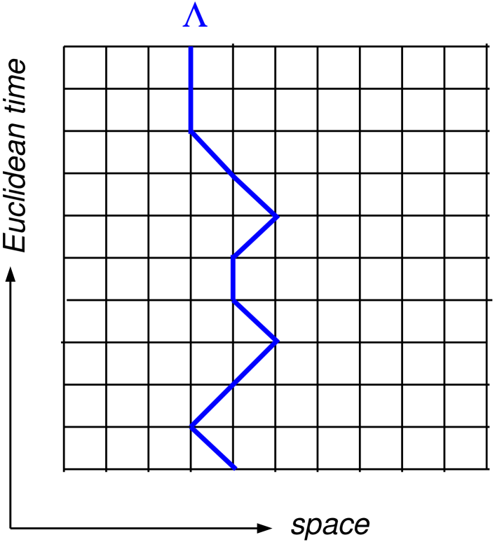
Figure 1: Illustration of the hyperon worldline. In the reduced transfer matrix formalism, the hyperon has been “integrated out”, and the interaction between the hyperon and the nucleons is mediated by an effective “background field” generated by the hyperon worldline.

For the non-interacting worldline, we can generate new configurations from the free probabilities, as determined from the reduced transfer matrices. In this case, $P_{h}=h$ is the hopping probability, and $P_{s}=(1-6h)$ is the probability to remain stationary. When initializing the worldline at the beginning of the MC simulation, we may start from a configuration where the worldline is completely stationary (“cold start”) or one where the worldline either hops or remains stationary at each time step according to the probabilities $P_{h}$ and $P_{s}$ (“warm start”).

At the beginning of every sweep through the lattice, we propose a new worldline to use for that sweep. This is done by taking the previous worldline and choosing a random time at which we cut the worldline and regenerating it either in the forwards and backwards time direction. The new worldline is then accepted or rejected using a Metropolis accept or reject condition to preserve detailed balance associated with the absolute value of the amplitude.

6 Results

For the results presented in what follows, we use a spatial lattice spacing $a=1/$(100 MeV) and temporal lattice spacing of $a_{t}=1/$(300 MeV). The non-local smearing parameter is chosen to be $s_{\rm NL}=0.2$, and the local smearing parameter is set to $s_{\rm L}=0.0$. Since we only consider $s$-shell nuclei and hypernuclei in this study, the local attraction provided by $s_{\rm L}$ for heavier nuclei is not needed Elhatisari:2016owd . The coupling constant $C_{NN}$ is set to $-7.5\times 10^{-6}$ MeV^-2, and this combination of parameters yields a nucleon-nucleon scattering length $a_{NN}=6.86$ fm and effective range $r_{NN}=1.77$ fm. The scattering length and effective range are calculated using Lüscher’s finite volume method Luscher:1990ux , as described in the Appendix of Ref. Lee:2007ae . We find that these parameters produce good results for the average $S$-wave phase shifts as well as the three- and four-nucleon binding energies. The exact transfer matrix calculation of the three-nucleon system and the Monte Carlo calculation of the four-nucleon system are both described in the following paragraphs. As stated previously, in this study the spin-dependent terms of the nucleon-nucleon interaction are not accounted for.

For the $YN$ interaction, we set $C_{YN}$ according to the best overall fit to the light hypernuclei. Fitting to the $\Lambda$ separation energies for ${}^{3}_{\Lambda}$H, ${}^{4}_{\Lambda}$H/He, and ${}^{5}_{\Lambda}$He, we find $C_{YN}=-1.6\times 10^{-5}$ MeV^-2. This gives $a_{YN}=-0.45$ fm for the scattering length and $r_{YN}=-0.45$ fm for the effective range. In Table 1, we present benchmark calculations of the ILMC results for ${}^{3}_{\Lambda}$H in comparison with exact transfer matrix calculations. We show the results for the energy as a function of Euclidean projection time.

Table 1: ILMC results for the energy of ${}^{3}_{\Lambda}$H versus Euclidean time in comparison with exact transfer matrix results for periodic box length 15.8 fm.

$N_{t}$	$t$ (MeV-1)	ILMC (MeV)	Exact (MeV)
50	0.1667	$-$1.0878(6)	$-$1.0878
100	0.3333	$-$1.4598(9)	$-$1.4590
150	0.5000	$-$1.6778(11)	$-$1.6760
200	0.6667	$-$1.7975(13)	$-$1.7966
250	0.8333	$-$1.8630(17)	$-$1.8614
300	1.0000	$-$1.8971(18)	$-$1.8954

We see that the agreement is quite good. The initial/final nucleon trial states for these calculations are taken to be spatially constant functions, which correspond to single-particle states of zero momentum in a periodic cubic box. The hyperon initial/final wave function is also taken be a constant function. Since we use a constant initial/final state wave function for the hyperon, the initial/final positions for the hyperon worldline are irrelevant in the Monte Carlo updating process. These exact transfer matrix calculations include the induced three-baryon interaction described in Eq. (46).

In Table 2, we present exact Lanczos transfer matrix calculations of the ground state of ²H, ${}^{3}_{\Lambda}$H, and separation energy $B_{\Lambda}$, as a function of periodic box length. In this work, we also present the exact Lanczos transfer matrix calculation wherever it is computationally possible and using Monte Carlo for cases where it is not. Given the extremely small $\Lambda$ separation energy, it is necessary to go to very large volumes in order to remove finite volume artifacts. Interestingly, $B_{\Lambda}$ is found to be relatively constant with the periodic box size $L$. This suppression of the finite volume dependence is an indication that the asymptotic normalization coefficient of the hypertriton wave function is small Konig:2011nz ; Konig:2017krd .

Table 2: Exact transfer matrix results for ²H, ${}^{3}_{\Lambda}$H, and the separation energy $B_{\Lambda}$ versus periodic box length.

$L$ (fm)	2H (MeV)	${}^{3}_{\Lambda}$H (MeV)	$B_{\Lambda}$ (MeV)
15.8	$-$1.651	$-$1.932	0.281
17.8	$-$1.460	$-$1.712	0.252
19.7	$-$1.332	$-$1.569	0.237
21.7	$-$1.245	$-$1.474	0.228
23.7	$-$1.186	$-$1.410	0.224
25.6	$-$1.146	$-$1.368	0.222
27.6	$-$1.118	$-$1.339	0.221
29.6	$-$1.100	$-$1.319	0.220

In Fig. 2, we present ILMC results for the ${}^{4}_{\Lambda}$H/He energy versus Euclidean time. These calculations use a periodic box size of $L=15.8$ fm with up to $N_{t}=300$ Euclidean time steps. In order to extract the ground state energy, we use the extrapolation ansatz

$$E(t)=E_{0}+c\exp(-\Delta Et),$$ (60)

which takes into account the residual dependence of the first excited state that couples to our initial/final states. For this calculation, we use an initial/final state where the nucleon states have a spatially decaying exponential form with respect to the nucleus center of mass, while the initial/final hyperon wave function is a constant function. It suffices to have an initial/final state with some overlap with the ground state wave function, and we find that these choices work very well.

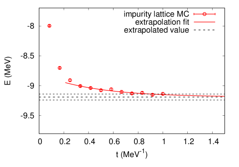
Figure 2: ILMC results for the ${}^{4}_{\Lambda}$H/He energy versus Euclidean projection time in a periodic box size of $L=15.8$ fm. We extract the ground state energy using an exponential ansatz for the asymptotic time dependence.

In Fig. 3, we show lattice Monte Carlo (LMC) results for the ⁴He energy versus Euclidean time. As there are no hyperons in this system, these are auxiliary field Monte Carlo calculations without impurity worldlines. These calculations use a periodic box size of $L=9.9$ fm with up to $N_{t}=150$ Euclidean time steps. In order to extract the ground state energy, we again use the exponential ansatz in Eq. (60). For this calculation, we again use an initial/final state where the nucleons have a spatially-decaying exponential form with respect to the nucleus center of mass.

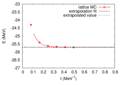
Figure 3: LMC results for the ⁴He energy versus Euclidean projection time in a periodic box size of $L=9.9$ fm. We extract the ground state energy using an exponential ansatz for the asymptotic time dependence.

In Fig. 4, ILMC results are shown for the ${}^{5}_{\Lambda}$He energy versus Euclidean time. These calculations use a periodic box size of $L=9.9$ fm with up to $N_{t}=250$ Euclidean time steps. We again use the exponential ansatz from Eq. (60) to extract the ground state energy. Similar to the ${}^{4}_{\Lambda}$H/He calculation, here we use an initial/final state where the nucleons have a spatially decaying exponential form with respect to the nucleus center of mass, while the initial/final hyperon wave function is a constant function.

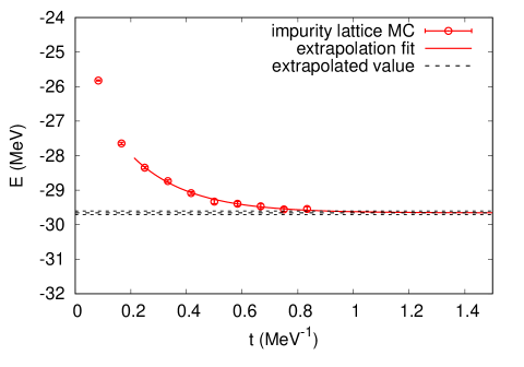
Figure 4: ILMC results for the ${}^{5}_{\Lambda}$He energy versus Euclidean time in a periodic box size of $L=9.9$ fm. We extract the ground state energy using an exponential ansatz for the asymptotic time dependence.

In Table 3, we present the lattice results for all of the $s$-shell nuclei and hypernuclei. The exact transfer matrix results are shown without error bars, while the ILMC and LMC results are shown with error bars that take into account stochastic errors and extrapolation errors. There is also a residual systematic error due to finite volume effects. For a box size of $L=29.6$ fm, the finite volume error on ²H is $0.04$ MeV, and the estimated finite volume error for ${}^{3}_{\Lambda}$H is also $\simeq 0.04$ MeV. As both corrections are in the same direction (with more binding at finite volume), the resulting finite volume error on the separation energy is $<0.002$ MeV.

For a box size of $L=15.8$ fm, the finite volume error on ³H/He is $\simeq 0.10$ MeV, and the estimated finite volume errors for ${}^{4}_{\Lambda}$H/He are also $\simeq 0.10$ MeV. For a box size of $L=9.9$ fm, the finite volume error on ⁴He is $\simeq 1.5$ MeV, and the estimated finite volume errors for ${}^{4}_{\Lambda}$H/He are $\simeq 2.0$ MeV.

Table 3: Summary of lattice results (exact transfer matrix, ILMC and LMC) for the energies of light nuclei and hypernuclei, and for separation energies. Comparisons with experimental separation energies are given where such data exists. These comparisons are averaged over Wigner SU(4) and $\Lambda$ spin components. For the case of ${}^{4}_{\Lambda}$H/He, we average over the $0^{+}$ and $1^{+}$ separation energies for ${}^{4}_{\Lambda}$H and ${}^{4}_{\Lambda}$He weighted by number of spin components. More data can be found in the review Ref. Davis:2005mb .

Nucleus $L$ (fm) $E$ (MeV) $B_{\Lambda}$ (MeV) $B^{\rm exp}_{\Lambda}$ (MeV) ²H 29.6 $-$1.100 – – ${}^{3}_{\Lambda}$H 29.6 $-$1.319 0.220 0.13(5) Bohm:1968qkc ; Juric:1973zq ; Davis:1991zpu ³H/He 15.8 $-$8.725 – – ${}^{4}_{\Lambda}$H/He 15.8 $-$9.19(5) 0.46(5) 1.39(4) Bohm:1968qkc ; Juric:1973zq ; Davis:1991zpu ; Bamberger:1973ht ; Bedjidian:1979qh ⁴He 9.9 $-$25.698(9) – – ${}^{5}_{\Lambda}$He 9.9 $-$29.66(6) 3.96(6) 3.12(2) Bohm:1968qkc ; Juric:1973zq ; Davis:1991zpu

For the comparison with the experimental results, we average over Wigner SU(4) and $\Lambda$ spin components where data exists. We see that while the $B^{\rm exp}_{\Lambda}$ is larger than the experimental values for ${}^{3}_{\Lambda}$H and ${}^{5}_{\Lambda}$He, the separation is smaller than experimental value for ${}^{4}_{\Lambda}$H/He. This is an indication that there are deficiencies in our very simple treatment of the $YN$ and $NN$ interactions. However, this serves as a good starting point for determining the essential features of the $YN$ interactions needed to describe the structure and properties of hypernuclei.

7 Discussion

We have shown, as a proof of principle, how state-of-the-art NLEFT calculations can be extended to include hyperons. As the number of hyperons in realistic hypernuclei is small (typically one or two) relative to the number of nucleons, we have applied the ILMC method whereby the hyperon “impurity” is integrated out and represented by a hyperon “worldline”, the position of which is updated during the MC calculation. Effectively, the standard NLEFT calculations for nucleons are augmented by a “background field” induced by the hyperon worldline. We have benchmarked the ILMC method by presenting preliminary MC results for the $s$-shell hypernuclei, using a simplified interaction similar to pionless EFT.

One of the most promising aspects of this work is the fact that the ILMC simulations scale very favorably with the number of nucleons. We have found that nearly all of the computational effort is consumed in calculating single-nucleon amplitudes as a function of the auxiliary field. As this part of the code scales linearly with the number of nucleons, it should be possible to perform calculations of hypernuclei with up to one hundred or more nucleons. We note also that the particular set of interactions that we have used here can also be directly applied to studying the properties of a bosonic impurity immersed in a superfluid Fermi gas. By modifying the included $P$-wave interactions of the impurity, we would also be able to describe the properties of an alpha particle immersed in a gas of superfluid neutrons. The possible applications of this method clearly go well beyond hypernuclear structure calculations and have general utility for numerous quantum many-body systems.

Returning to hypernuclear systems, the obvious next extension of this work is to include spin-dependent $YN$ interactions. The importance of the spin-dependence of the $YN$ interaction can be seen clearly in the splittings between the $0^{+}$ and $1^{+}$ states in ${}^{4}_{\Lambda}$H and ${}^{4}_{\Lambda}$He Ref. Gibson:1995an . One should also include explicit $\Lambda N$-$\Sigma N$ transitions, see e.g. Beane:2003yx , as well as one-meson exchange interactions that would put the $YN$ interaction in the same EFT formalism Haidenbauer:2013oca ; Haidenbauer:2019boi as currently used for the $NN$ interaction in NLEFT Li:2018ymw .

The number of adjustable parameters in the $YN$ interaction will then increase. The most natural approach, in line with the treatment of the $NN$ interaction, would be to fit such parameters to $\Lambda N$ scattering phase shifts. However, due to the paucity of such data (especially at low energies), we expect to need at least the hypertriton binding energy as an additional constraint, as it is also done in continuum chiral EFT, see e.g. Ref. Haidenbauer:2019boi . As the effects of $\Lambda N$-$\Sigma N$ transitions are included, it may be necessary to use further empirical data on other light hypernuclei to constrain the relevant LECs. A further extension concerns the extension to $S=-2$ hypernuclei, which on the one hand would involve the $YY$ interactions Polinder:2007mp ; Haidenbauer:2015zqb ; Hiyama:2018lgs and on the other hand a modified ILMC algorithm for two interacting worldlines. Work along these lines is underway.

References

- (1) C. Korpa, A. Dieperink and R. Timmermans, Phys. Rev. C 65 (2002) 015208.
- (2) H. Polinder, J. Haidenbauer and U.-G. Meißner, Nucl. Phys. A 779 (2006) 244.
- (3) D. Lee, Prog. Part. Nucl. Phys. 63 (2009) 117.
- (4) T. A. Lähde and U.-G. Meißner, Lect. Notes Phys. 957 (2019), 1.
- (5) J. Haidenbauer, S. Petschauer, N. Kaiser, U.-G. Meißner, A. Nogga and W. Weise, Nucl. Phys. A 915 (2013) 24.
- (6) J. Haidenbauer, U.-G. Meißner and A. Nogga, Eur. Phys. J. A 56 (2020) 91.
- (7) D. Lonardoni, S. Gandolfi and F. Pederiva, Phys. Rev. C 87 (2013) 041303.
- (8) D. Gazda and A. Gal, Nucl. Phys. A 954 (2016) 161.
- (9) R. Wirth and R. Roth, Phys. Lett. B 779 (2018) 336.
- (10) R. Wirth, D. Gazda, P. Navrátil and R. Roth, Phys. Rev. C 97 (2018) 064315.
- (11) H. Le, J. Haidenbauer, U.-G. Meißner and A. Nogga, Phys. Lett. B 801 (2020) 135189.
- (12) J. Haidenbauer and I. Vidana, Eur. Phys. J. A 56 (2020) 55.
- (13) S. Bour, MSc thesis, University of Bonn (2009).
- (14) M. L. Wagman, F. Winter, E. Chang, Z. Davoudi, W. Detmold, K. Orginos, M. J. Savage and P. E. Shanahan, Phys. Rev. D 96 (2017) 114510
- (15) S. Elhatisari and D. Lee, Phys. Rev. C 90 (2014) 064001.
- (16) S. Bour, D. Lee, H. W. Hammer and U.-G. Meißner, Phys. Rev. Lett. 115 (2015) 185301
- (17) B. N. Lu, N. Li, S. Elhatisari, D. Lee, E. Epelbaum and U.-G. Meißner, Phys. Lett. B 797 (2019) 134863.
- (18) H. Hammer, Nucl. Phys. A 705 (2002) 173.
- (19) L. Contessi, N. Barnea and A. Gal, Phys. Rev. Lett. 121 (2018) 102502.
- (20) S. Elhatisari et al., Phys. Rev. Lett. 117 (2016) 132501.
- (21) S. Elhatisari et al., Phys. Rev. Lett. 119 (2017) 222505.
- (22) N. Li, S. Elhatisari, E. Epelbaum, D. Lee, B. N. Lu and U.-G. Meißner, Phys. Rev. C 98 (2018) 044002.
- (23) E. Wigner, Phys. Rev. 51 (1937) 106.
- (24) M. Lüscher, Nucl. Phys. B 354 (1991) 531.
- (25) D. Lee, Eur. Phys. J. A 35 (2008) 171.
- (26) S. König, D. Lee and H. W. Hammer, Phys. Rev. Lett. 107 (2011) 112001.
- (27) S. König and D. Lee, Phys. Lett. B 779 (2018) 9.
- (28) B. F. Gibson and E. V. Hungerford, Phys. Rept. 257 (1995) 349.
- (29) G. Bohm, et al., Nucl. Phys. B 4 (1968) 511.
- (30) M. Juric, et al., Nucl. Phys. B 52 (1973) 1.
- (31) D. H. Davis, AIP Conf. Proc. 224 (1991) 38.
- (32) A. Bamberger et al. [CERN-Heidelberg-Warsaw], Nucl. Phys. B 60 (1973) 1.
- (33) M. Bedjidian et al. [CERN-Lyon-Warsaw], Phys. Lett. B 83 (1979) 252.
- (34) D. H. Davis, Nucl. Phys. A 754 (2005) 3.
- (35) S. Beane, P. Bedaque, A. Parreno and M. Savage, Nucl. Phys. A 747 (2005) 55.
- (36) H. Polinder, J. Haidenbauer and U.-G. Meißner, Phys. Lett. B 653 (2007) 29.
- (37) J. Haidenbauer, U.-G. Meißner and S. Petschauer, Nucl. Phys. A 954 (2016) 273.
- (38) E. Hiyama and K. Nakazawa, Ann. Rev. Nucl. Part. Sci. 68 (2018) 131.