Mixed-state entanglement from local randomized measurements

Abstract

We propose a method for detecting bipartite entanglement in a many-body mixed state based on estimating moments of the partially transposed density matrix. The estimates are obtained by performing local random measurements on the state, followed by post-processing using the classical shadows framework. Our method can be applied to any quantum system with single-qubit control. We provide a detailed analysis of the required number of experimental runs, and demonstrate the protocol using existing experimental data [Brydges et al, Science 364, 260 (2019)].

Engineered quantum many-body systems exist in today’s laboratories as Noisy Intermediate Scale Quantum Devices (NISQ) Preskill (2018). This provides us with novel opportunities to study and quantify entanglement – a fundamental concept in both quantum information theory Horodecki et al. (2009) and many-body quantum physics Eisert et al. (2010); Calabrese and Cardy (2016). For pure (or nearly-pure) states, entanglement has been detected by measuring the second Rényi entropy  Horodecki and Horodecki (1996); Horodecki (2003); Islam et al. (2015); Kaufman et al. (2016); Linke et al. (2018); Brydges et al. (2019). This has been achieved via, for instance, many-body quantum interference Alves and Jaksch (2004); Daley et al. (2012); Islam et al. (2015); Kaufman et al. (2016); Linke et al. (2018) (see also Cardy (2011); Abanin and Demler (2012)) and randomized measurements van Enk and Beenakker (2012); Elben et al. (2018, 2019); Brydges et al. (2019); Huang et al. (2020). However, many states of interest are actually highly mixed – either because of decoherence, or because they describe interesting subregions of a larger, globally entangled, system. Developing protocols which detect and quantify mixed-state entanglement on intermediate scale quantum devices is thus an outstanding challenge.

Below we propose and experimentally demonstrate conditions for mixed-state entanglement and measurement protocols based on the positive partial transpose (PPT) condition Peres (1996); Horodecki and Horodecki (1996); Horodecki et al. (2009). Consider two partitions $A$ and $B$ described by a (reduced) density matrix $\rho_{AB}$. The well-known PPT condition checks if the partially transposed (PT) density matrix $\rho_{AB}^{T_{A}}$ is positive semidefinite, i.e. all eigenvalues are non-negative. If the PPT condition is violated – i.e. $\rho_{AB}^{T_{A}}$ does have negative eigenvalues – $A$ and $B$ must be entangled. It is possible to turn the PPT condition into a quantitative entanglement measure. The negativity $\mathcal{N}(\rho_{AB})=\sum_{\lambda<0}|\lambda|$, with $\lambda$ the spectrum of $\rho_{AB}^{T_{A}}$, is positive if and only if the underlying state $\rho_{AB}$ violates the PPT condition Vidal and Werner (2002). While applicable to mixed states, computing the negativity requires accurately estimating the full spectrum of $\rho_{AB}^{T_{A}}$. We bypass this challenge by considering moments of the partially transposed density matrix (PT-moments) instead:

$$p_{n}=\mathrm{Tr}[(\rho_{AB}^{T_{A}})^{n}]\quad\text{for $n=1,2,3,\ldots$}.$$ (1)

These have been first studied in quantum field theory to quantify correlations in many-body systems Calabrese et al. (2012). Clearly, $p_{1}=\mathrm{tr}(\rho_{AB})=1$, while $p_{2}$ is equal to the purity $\mathrm{tr}[\rho_{AB}^{2}]$ (see Table 1 in the Supplemental Material SM (SM) for a visual derivation). Hence, $p_{3}$ is the lowest PT-moment that captures meaningful information about the partial transpose (see also Ref. Gray et al. (2018)).

In this letter, we first show that the first three PT-moments can be used to define a simple yet powerful test for bipartite entanglement:

$$\rho_{AB}\in\mathrm{PPT}\implies p_{3}\geq p_{2}^{2}.$$ (2)

The $p_{3}$-PPT condition is the contrapositive of this assertion: if $p_{3}<p_{2}^{2}$, then $\rho_{AB}$ violates the PPT condition [see Fig. 1a)] and must therefore be entangled (see SM SM for the proof). Similar to the PPT condition, the $p_{3}$-PPT condition applies to mixed states and is completely independent of the state in question. This is a key distinction from entanglement witnesses Terhal (2000); Gühne and Lütkenhaus (2006), which can be more powerful, but which usually require detailed prior information about the state. While in general weaker than the full PPT condition, the $p_{3}$-PPT condition relies on comparing two comparatively simple functionals and outperforms other state-independent entanglement detection protocols, like comparing purities of various nested subsystems Horodecki and Horodecki (1996); Islam et al. (2015); Kaufman et al. (2016); Linke et al. (2018); Brydges et al. (2019); SM . As shown in the SM SM , the $p_{3}$-PPT condition becomes equivalent to the PPT condition for Werner states (in this case, it is a necessary and sufficient condition for bipartite entanglement Watrous (2018)).

The second main contribution of this letter is a measurement protocol to determine PT-moments in NISQ devices.

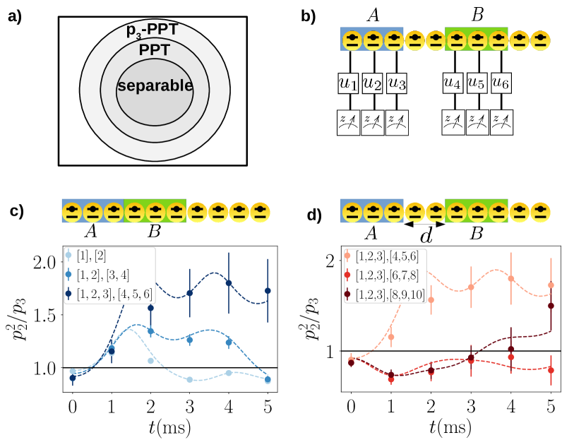
Figure 1: Protocol and illustrations. a) The $p_{3}$-PPT condition can be used to demonstrate mixed-state bipartite entanglement with PT-moments. Separable states are PPT states and also fulfill the $p_{3}$-PPT condition. Thus, quantum states which violate the $p_{3}$-PPT condition must be bipartite entangled [see also Eq. (2)]. b) In our protocol, PT-moments are measured by applying local random unitaries followed by computational basis measurements. c-d) Violation of the $p_{3}$-PPT condition, i.e. $p_{2}^{2}>p_{3}$, is experimentally observed for connected c) and disconnected (separated by $d=0,2,4$ spins) d) partitions $A$ and $B$ at various times $t$ after a quantum quench Brydges et al. (2019). Dots: experimental results. Error bars: Jackknife estimates of statistical errors. Lines: numerical simulations including the decoherence model presented in Ref. Brydges et al. (2019).

Crucially, we employ randomized measurements implemented with local (single-qubit) random unitaries, see Fig. 1b) which are readily available in NISQ devices and have been already successfully applied to measure entanglement entropies, many-body state-fidelities, and out-of-time ordered correlators Brydges et al. (2019); Mi et al. (2020); Elben et al. (2020a); Joshi et al. (2020). In contrast to previous proposals for measuring PT-moments, our protocol does not rely on many-body interference between identical state copies Horodecki (2003); Gray et al. (2018); Cornfeld et al. (2019), or on using global entangling random unitaries Zhou et al. (2020) built from interacting Hamiltonians Dankert et al. (2009); Nakata et al. (2017); Elben et al. (2018); Vermersch et al. (2018). Instead, it only requires single-qubit control, and allows for the estimation of many distinct PT-moments from the same data. In particular, arbitrary orders $n\geq 2$ and arbitrary (connected, as well as disconnected) partitions $A$, $B$ can be measured.

While the experimental setup for our measurement protocol is reminiscent of quantum state tomography Gross et al. (2010); Cramer et al. (2010); Torlai et al. (2018); Guţă et al. (2020), there are fundamental differences regarding the required number of measurements (as independent state copies), and the way the measured data is processed. Without strong assumptions on the state Cramer et al. (2010); Torlai et al. (2018), performing tomography to infer an $\epsilon$-approximation of an unknown density matrix $\rho_{AB}$ (e.g. in order to subsequently compute $\epsilon$-approximations of $p_{n}$) requires (at least) order $2^{|AB|}\mathrm{rank}(\rho_{AB})/\epsilon^{2}$ measurements Haah et al. (2017); O’Donnell and Wright (2016). In the high accuracy regime ($\epsilon\ll 1$), our direct estimation protocol instead only requires order $2^{|AB|}/\epsilon^{2}$ measurements. For highly mixed states – the central topic of this work – this discrepancy heralds a significant reduction in measurement resources. Furthermore, we predict PT-moments through a ’direct’ and (multi-) linear postprocessing of the measurement data represented as ’classical shadows’ Huang et al. (2020). Thus, data processing is cheap – both in memory and runtime – and can be massively parallelized. Similar to previous measurement van Enk and Beenakker (2012); Elben et al. (2018); Brydges et al. (2019); Vermersch et al. (2019); Joshi et al. (2020); Elben et al. (2020a, b); Huang et al. (2020); Cian et al. (2020) and entanglement detection Tran et al. (2015, 2016); Ketterer et al. (2019); Zhang et al. (2020); Knips et al. (2020) protocols based on randomized measurements, this is another distinct advantage over tomography which typically requires expensive data-processing algorithms Gross et al. (2010) or training a neural network Torlai et al. (2018).

Finally, we demonstrate our measurement protocol and the $p_{3}$-PPT condition experimentally in the context of the quantum simulation of many-body systems. Here, PT-moments have been shown to reveal universal properties of quantum phases of matter Calabrese et al. (2012, 2013); Ruggiero et al. (2016); Javanmard et al. (2018); Turkeshi et al. (2020) and their transitions Calabrese et al. (2012, 2013); Chung et al. (2014); Wu et al. . Out of equilibrium, PT-moments allow to understand the dynamical process of thermalization Coser et al. (2014); Alba and Calabrese (2019a); Kudler-Flam et al. (2020); Alba and Carollo , and the fate of (many-body) localization in presence of decoherence Wybo et al. . In this work, we analyze the data of Ref. Brydges et al. (2019) corresponding to the out-of-equilibrium dynamics in a spin model with long-range interactions, which was implemented in a $10$-qubit trapped ion quantum simulator. In particular, we certify the presence of mixed-state entanglement via the $p_{3}$-PPT condition [see Fig. 1(c-d), and for details below]. Furthermore, we monitor the time-evolution of $p_{3}$ and observe dynamical signatures of entanglement spreading and thermalization Coser et al. (2014); Alba and Calabrese (2019a).

Protocol– The experimental ingredients to measure PT-moments build on resources similar to the ones presented in Ref. Elben et al. (2018) and realized in Ref. Brydges et al. (2019) to measure Rényi entropies. The key new element is the post-processing of the experimental data Huang et al. (2020). As shown in Fig. 1, the quantum state of interest is realized in a system of $N$ qubits. In the partitions $A$ and $B$, consisting of $|A|$ and $|B|$ spins, respectively, a randomized measurement is performed by applying random local unitaries $u=u_{1}\otimes\dots\otimes u_{|AB|}$, with $u_{i}$ independent single qubit rotation sampled from a unitary $3$-design Gross et al. (2007); Dankert et al. (2009), and a subsequent projective measurement in the computational basis with outcome $\mathbf{k}=(k_{1},\dots,k_{|AB|})$. This is subsequently repeated with $M$ different random unitaries such that a data set of $M$ bitstrings $\mathbf{k}^{(r)}$ with $r=1,\dots,M$ is collected.

From this data set, the PT-moments $p_{n}$ can be estimated without having to reconstruct the density matrix $\rho_{AB}$, and with a significantly smaller number of experimental runs $M$ than required for full quantum state tomography. To obtain such estimates, we rely on two observations. First, each outcome $\mathbf{k}^{(r)}$ can be used to define an unbiased estimator

$$\hat{\rho}_{AB}^{(r)}=\bigotimes_{i\in AB}\left[3(u_{i}^{(r)})^{\dagger}\ket{k_{i}^{(r)}}\bra{k_{i}^{(r)}}u_{i}^{(r)}-\mathbb{I}_{2}\right]$$ (3)

of the density matrix $\rho_{AB}$, i.e. $\mathbb{E}[\hat{\rho}_{AB}^{(r)}]=\rho_{AB}$ with the expectation value taken over the unitary ensemble and projective measurements Ohliger et al. (2013); Elben et al. (2019); Paini and Kalev ; Huang et al. (2020). Second, the PT-moments $p_{n}$ can be viewed as an expectation value of a $n$-copy observable $\overrightarrow{\Pi}_{A}\,\overleftarrow{\Pi}_{B}$ evaluated on $n$-copies of the original density matrix $\rho_{AB}$,

$$p_{n}=\mathrm{Tr}\left[\overrightarrow{\Pi}_{A}\,\overleftarrow{\Pi}_{B}\,\rho_{AB}^{\otimes n}\right].$$ (4)

Here, $\overrightarrow{\Pi}_{A}$ and $\overleftarrow{\Pi}_{B}$ are $n$-copy cyclic permutation operators $\overrightarrow{\Pi}_{A}\ket{\mathbf{k}^{[1]}_{A},\mathbf{k}^{[2]}_{A},\dots,\mathbf{k}^{[n]}_{A}}=\ket{\mathbf{k}^{[n]}_{A},\mathbf{k}^{[1]}_{A},\dots,\mathbf{k}^{[n-1]}_{A}}$, $\overleftarrow{\Pi}_{B}\ket{\mathbf{k}^{[1]}_{B},\mathbf{k}^{[2]}_{B},\dots,\mathbf{k}^{[n]}_{B}}=\ket{\mathbf{k}^{[2]}_{B},\dots,\mathbf{k}^{[n]}_{B},\mathbf{k}^{[1]}_{B}}$ that act on the partitions $A$ and $B$, respectively.

Estimators of the PT-moments $p_{n}$ can now be derived from Eqs. (3) and (4) using U-statistics Hoeffding (1992). Replacing $\rho^{\otimes n}$ with $\hat{\rho}^{(r_{1})}\otimes\dots\otimes\hat{\rho}^{(r_{n})}$ where $r_{1}\neq r_{2}\neq\dots\neq r_{n}$, corresponding to independently sampled random unitaries $u^{(r_{1})},\dots,u^{(r_{n})}$, we define the U-statistic

$$\hat{p}_{n}=\frac{1}{n!}\binom{M}{n}^{-1}\!\!\!\sum_{\begin{subarray}{c}r_{1}\neq r_{2}\neq\dots\neq r_{n}\end{subarray}}\!\!\!\mathrm{Tr}\left[\overrightarrow{\Pi}_{A}\,\overleftarrow{\Pi}_{B}\hat{\rho}_{AB}^{(r_{1})}\otimes\dots\otimes\hat{\rho}_{AB}^{(r_{n})}\right].$$ (5)

It follows from the defining properties of $U$-statistics that $\hat{p}_{n}$ is an unbiased estimator of $p_{n}$, i.e. $\mathbb{E}[\hat{p}_{n}]=p_{n}$ with the expectation value taken over the unitary ensemble and projective measurements Hoeffding (1992). Its variance governs the statistical errors arising from finite $M$. Furthermore, a quick inspection of Eqs. (3) and (4) reveals that the summands in Eq. (5) completely factorize into contractions of single qubit matrices, $\mathrm{Tr}[\overrightarrow{\Pi}_{A}\,\overleftarrow{\Pi}_{B}\hat{\rho}_{AB}^{(r_{1})}\otimes\dots\otimes\hat{\rho}_{AB}^{(r_{n})}]=\Pi_{i\in A}\mathrm{Tr}[\hat{\rho}_{i}^{(r_{1}),T}\cdots\hat{\rho}_{i}^{(r_{n}),T}]\Pi_{i\in B}\mathrm{Tr}[\hat{\rho}_{i}^{(r_{1})}\cdots\hat{\rho}_{i}^{(r_{n})}]$, with $\hat{\rho}_{AB}^{(r)}=\otimes_{i\in AB}\hat{\rho}^{(r)}_{i}$ as in Eq. (3). Thus, given $M$ observed bitstrings $\mathbf{k}_{r}$, one can determine $\hat{p}_{n}$ with classical data processing scaling as $M^{n}|AB|$, without storing exponentially large matrices on the classical post-processing device.

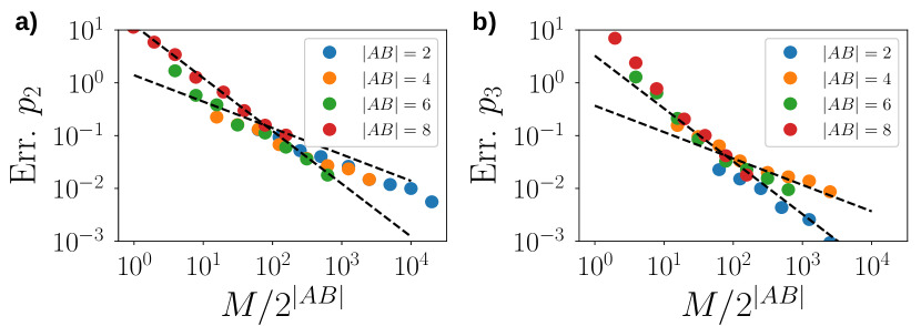
Figure 2: Statistical errors for the GHZ state. Dashed lines represent scalings of $\propto 1/M$, and $\propto 1/\sqrt{M}$. In both cases, the number of measurements to estimate $p_{2}$ a) and $p_{3}$ b) with accuracy $~{}0.1$ is of the order of $100\times 2^{|AB|}$.

Statistical errors– As demonstrated in Fig. 1(c,d), PT-moments can be inferred using a finite number of experimental runs $M$. Here, we investigate in detail the statistical errors arising from the finite value of $M$.

Analytically, we bound statistical errors based on the variance of the multi-copy observable in question. For $p_{2}=\mathrm{Tr}[(\rho_{AB}^{T_{A}})^{2}]$, our analysis reveals that the error decay rate depends on number of measurements $M$. In the large $M$ regime, the error is proportional to $2^{|AB|}p_{2}/\sqrt{M}$. This error bound is multiplicative – i.e. the size of the error is proportional to the size of the target $p_{2}$ – and $1/\sqrt{M}$ captures the expected decay rate for an estimation procedure that relies on empirical averaging. For small and intermediate values of $M$, the estimation error is instead bounded by $8\times 2^{1.5|AB|}/M$. While this is worse in terms of constants, the error decays at a much faster rate proportional to $1/M$. Qualitatively similar results apply for estimating $p_{3}=\mathrm{Tr}[(\rho_{AB}^{T_{A}})^{3}]$, but there can be three decay regimes. For large $M$, the estimation error is bounded by $2^{|AB|}p_{2}^{2}/\sqrt{M}$. This again captures the asymptotically optimal rate $1/\sqrt{M}$ associated with empirical averaging, but the constant is suppressed by $p_{2}^{2}$, not $p_{3}$ itself. For intermediate $M$, the error decay rate is proportional to $1/M$, while an even faster rate $\propto 1/M^{3/2}$ governs the error decay for small $M$. We refer to the SM for detailed statements and proofs.

Now, we test these predictions numerically by simulating the experimental protocol for various values of $M$ in systems with $N=|AB|$ qubits where a pure GHZ state $\rho=\ket{\phi_{\text{GHZ}}}\!\bra{\phi_{\text{GHZ}}}$ is prepared. Here, $A$ corresponds to the first $N/2$ qubits, and $B$ is the complement. The results are shown in Fig. 2 and support our analytical error bounds. They highlight in particular that the number of measurement repetitions necessary to achieve a desired accuracy of $\sim 0.1$ scales as $2^{|AB|}$. This enables the estimation of PT-moments in state of the art platforms with high repetition rates. These findings are discussed and confirmed for the ground state of the transverse Ising model in the SM SM .

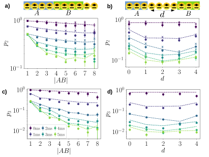
Figure 3: Reconstruction of $p_{2}=\mathrm{Tr}[(\rho_{AB}^{T_{A}})^{2}]$ and $p_{3}=\mathrm{Tr}[(\rho_{AB}^{T_{A}})^{3}]$ from experimental data Brydges et al. (2019). $A$ and $B$ are parts of a total system of 10 qubits. In a) and c), we take $A=[1,\dots,\lfloor|AB|/2\rfloor]$ and $B=[\lfloor|AB|/2\rfloor+1,\dots,|AB|]$. In b) and d), we take $A=\{1,2,3\}$ and $B=\{4+d,5+d,6+d\}$ with $d=0,1,\dots 4$. Dots are obtained with the shadow estimator [Eq. (5) second and third order], crosses with the direct estimator (second order) of Ref. Brydges et al. (2019). Different colors correspond to different times after the quantum quench with purple [0 ms] corresponding to the initial product state. For each time, $M=500$ unitaries and $P=150$ measurements per unitary were used. Lines: theory simulation including decoherence Brydges et al. (2019). The ratio $p_{2}^{2}/p_{3}$, detecting entanglement according to the $p_{3}$-PPT condition, is shown in Fig. 1 c) and d).

PT-moments in a trapped-ion quantum simulator–

Below, we discuss the experimental demonstration of the measurement of PT-moments in a trapped ion quantum simulator. To this end, we evaluate data taken in the context of Ref. Brydges et al. (2019). Here, the Rényi entropy growth in quench dynamics was investigated. The system, consisting in total of $N=10$ qubits, was initialized in the Néel state $\ket{\uparrow\downarrow\uparrow\downarrow\dots}$, and time-evolved with

$$H_{\mathrm{XY}}=\hbar\sum_{i<j}J_{ij}(\sigma^{+}_{i}\sigma^{-}_{j}+\sigma^{-}_{i}\sigma^{+}_{j})+\hbar B\sum_{i}\sigma^{z}_{i}$$ (6)

with $\sigma_{i}^{z}$ the third spin-$1/2$ Pauli operator, $\sigma_{i}^{+}(\sigma_{i}^{-})$ the spin-raising (lowering) operators acting on spin $i$, and $J_{ij}\approx J_{0}/\lvert{i-j}\rvert^{\alpha}$ the coupling matrix with an approximate power-law decay $\alpha\approx 1.24$ and $J_{0}=420s^{-1}$. After time evolution, randomized measurements were performed, using $M=500$ random unitaries and $P=150$ projective measurements per random unitary.

From this data, PT-moments can be inferred , with results presented in Fig. 3. For the purity $p_{2}$ a) b), we observe good agreement with theory for up to $N=8$ qubits partitions, in particular the raise of $p_{2}$ for partition sizes approaching the total system size which is expected for such nearly pure states. For $9$, $10$-qubit partitions, the data is not shown since the relative statistical error of the estimated data points approaches unity . We however note that the measured $\hat{p}_{2}$ is slightly underestimated. This is due to imperfect realizations of the random unitaries, which tend to reduce the estimation of the overlap $\mathrm{Tr}(\rho_{r_{1}}\rho_{r_{2}})$. This effect is also present when measuring cross-platform fidelities Elben et al. (2020a). For the third PT-moment $p_{3}$ c), d), we observe the same kind of agreement between theory value and experimental measurements. In particular, at large partition sizes, the protocol is able to measure with high precision small values of $p_{3}$. These small values are indeed fundamental to detect entanglement: a PPT violating state has a negative eigenvalue which reduces the value of $p_{3}$, in comparison with the purity $p_{2}$. This effect is mathematically captured by the $p_{3}$-PPT condition and allowed us to detect PPT violation and thus entanglement for many-body mixed states [see Fig. 1c)]. In the SM SM , we present additional simulations showing the power of the $p_{3}$-PPT condition, in comparison with the negativity and the condition based on purities of nested subsystems.

The third PT-moment $p_{3}$ does not only allow to detect mixed-state entanglement. It can also be used to study the dynamics of entanglement in various many-body quantum systems Calabrese et al. (2012); Chung et al. (2014); Coser et al. (2014); Wu et al. ; Wybo et al. . Here, we analyze the behavior of the dimensionless ratio $R_{3}=-\log_{2}[p_{3}/\mathrm{Tr}(\rho_{AB}^{3})]$, which, as shown in quantum field theory, follows the same universal behavior as the negativity during evolution with a local Hamiltonian Coser et al. (2014). We remark that $R_{3}$ is however only well-defined for states with $p_{3}>0$ (Werner states in large dimensions are a counter-example SM ). Furthermore, $R_{3}$ is not an entanglement monotone Wybo et al. . It vanishes for all product states, but can still be strictly positive for certain separable states Horodecki et al. (2009); Wybo et al. .

Fig. 4 illustrates the time evolution of $R_{3}$ for (a) connected and (b) disconnected subsystems $AB$, respectively. The appearing peaks of $R_{3}$ have been predicted and analyzed for various one-dimensional quantum systems subject to local interactions Coser et al. (2014); Alba and Calabrese (2019a) (and have also been studied in the context of Rényi mutual information Alba and Calabrese (2019b); Maity et al. (2020)). They can be understood in terms of propagating quasi-particles which describe collective excitations in the system Coser et al. (2014); Alba and Calabrese (2019a). In this picture, entanglement between two partitions $A$ and $B$ is induced by the presence of entangled pairs of quasi-particles shared between $A$ and $B$. For each pair, the individual quasi-particles propagate in opposite directions and start to entangle, in the course of the time evolution, partitions that are more and more separated Coser et al. (2014); Alba and Calabrese (2019a). In particular, for two adjacent partitions (a), $R_{3}$ increases at early times, which is consistent with the picture of shared pairs of entangled quasi-particles entering the two partitions immediately. After a certain time $R_{3}$ reaches a maximum and starts to decrease, which can be understood as the time when the quasi-particles start to ‘escape’ the region $AB$. For separated partitions (b), the peaks are delayed due to the finite speed of propagation of the quasi particles. In addition, their maximum value is lowered because of the finite life-times of quasi-particles. The latter feature is characteristic to chaotic (non-integrable) thermalizing systems Alba and Calabrese (2019b) and is in our case further enhanced by decoherence.

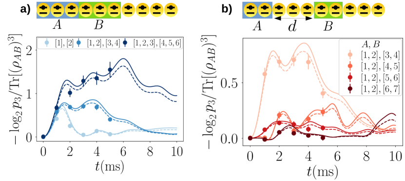
Figure 4: Evolution of the ratio $R_{3}$ from experimental data Brydges et al. (2019). (a) Connected partitions. (b) Disconnected partitions separated by $d=0,1,2,3$ spins. Different colors correspond to different partitions $AB$. Dots are obtained with the shadow estimator Eq. (5) using experimental data Brydges et al. (2019). Solid (dashed) lines: theory simulation of unitary dynamics (including decoherence Brydges et al. (2019)).

Conclusion– Our protocol extends the paradigm of randomized measurements, yielding the first direct measurement of PT-moments in a many-body system. U-statistics provides the key ingredient there and enables us to harness a remarkable advantage over state tomography in terms of statistical errors. At a fundamental level, it is therefore natural to investigate how to access new important physical quantities based on random measurement data, and with significant savings in terms of measurement and classical postprocessing over existing methods. This approach can be used to derive protocols to directly infer entanglement measures (including non-polynomial functions of the density matrix), such as the von-Neumann entropy and the negativity.

Appendix A The $p_{3}$-PPT condition

In this section we present, prove and discuss the $p_{3}$-PPT condition. The $p_{3}$-PPT condition is the contrapositive of the following statement about moments of positive semidefinite matrices with unit trace.

Proposition 1.

For every positive semidefinite matrix $X$ with unit trace ($\mathrm{Tr}(X)=1$) it holds that

$$\mathrm{tr}(X^{2})^{2}\leq\mathrm{tr}(X^{3}).$$ (7)

Note that Eq. (7) resembles the following well-known monotonicity relation among Rényi entropies (see e.g., Ref. Zyczkowski (2003)):

$$S_{3}(\rho)\leq S_{2}(\rho)\;\;\text{for}\;\;S_{n}(\rho)=\tfrac{1}{1-n}\log_{2}\big{(}\mathrm{tr}(\rho^{n})\big{)}.$$ (8)

However, this relation only applies to density matrices, i.e. positive semidefinite matrices with unit trace. The $p_{3}$-PPT condition, in contrast, is designed to test the absence of positive semidefiniteness. Hence, it is crucial to have a condition that does not break down if the matrix in question has negative eigenvalues. Rel. (7) (and its direct proof provided in the next subsection) do achieve this goal, while an argument based on monotonicity relations between Rényi entropies can break down, because the logarithm of non-positive numbers is not properly defined.

A.1 Proof of the $p_{3}$-PPT condition

Let $X$ be a Hermitian $d\times d$ matrix with eigenvalue decomposition $X=\sum_{i=1}^{d}\lambda_{i}|x_{i}\rangle\!\langle x_{i}|$. For $p\geq 1$, we introduce the Schatten-$p$ norms

$$\|X\|_{p}=\Big{(}\sum_{i=1}^{d}|\lambda_{i}|^{p}\Big{)}^{1/p}=\mathrm{Tr}\left(|X|^{p}\right)^{1/p},$$

where $|X|=\sqrt{X^{2}}=\sum_{i=1}^{d}|\lambda_{i}||x_{i}\rangle\!\langle x_{i}|$ denotes the (matrix-valued) absolute value. The Schatten-$p$ norms encompass most widely used matrix norms in quantum information. Concrete examples are the trace norm ($p=1$), the Hilbert-Schmidt/Frobenius norm ($p=2$) and the operator/spectral norm ($p=\infty$). Each Schatten-$p$ norm corresponds to the usual vector $\ell_{p}$-norm of the vector of eigenvalues $\lambda=(\lambda_{1},\ldots,\lambda_{d})^{T}\in\mathbb{R}^{d}$:

$$\|\lambda\|_{\ell_{p}}=\Big{(}\sum_{i=1}^{d}|\lambda_{i}|^{p}\Big{)}^{1/p}\quad\text{for $p\geq 1$.}$$ (9)

Hence, Schatten-$p$ norms inherit many desirable properties from their vector-norm counterparts. Here, we shall use vector norm relations to derive a relation among Schatten-$p$ norms. It is based on Hoelder’s inequality that relates the inner product

$$\langle v,w\rangle=\sum_{i=1}^{d}v_{i}w_{i}\quad\text{for $v,w\in\mathbb{R}^{d}$}$$ (10)

to a combination of $\ell_{p}$ norms.

Fact 1 (Hoelder’s inequality for vector norms).

Fix $p,q\geq 1$ such that $1/p+1/q=1$. Then,

$$\left|\langle v,w\rangle\right|\leq\sum_{i=1}^{d}|v_{i}w_{i}|\leq\|v\|_{\ell_{p}}\|w\|_{\ell_{q}}$$ (11)

for any $v,w\in\mathbb{R}^{d}$.

The well-known Cauchy-Schwarz inequality is a special case of this fact. Set $p=q=1/2$ to conclude

$$\left|\langle v,w\rangle\right|\leq\|v\|_{\ell_{2}}\|w\|_{\ell_{2}}=\langle v,v\rangle^{1/2}\langle w,w\rangle^{1/2}.$$ (12)

At the heart of our proof for the $p_{3}$-PPT condition is a simple relation between Schatten-$p$ norms of orders $p=1,2,3$.

Lemma 1.

The following norm relation holds for every Hermitian matrix $X$:

$$\|X\|_{2}^{4}\leq\|X\|_{1}\|X\|_{3}^{3}$$

Proof.

Let $\lambda=(\lambda_{1},\ldots,\lambda_{d})^{T}$ be the $d$-dimensional vector of eigenvalues of $X$. Apply Hoelder’s inequality with $p=3,q=3/2$ to the inner product of this vector of eigenvalues with itself:

$$\mathrm{Tr}(X^{2})=\langle\lambda,\lambda\rangle\leq\|\lambda\|_{\ell_{3}}\|\lambda\|_{\ell_{2/3}}=\|X\|_{3}\|\lambda\|_{\ell_{3/2}}.$$ (13)

Next, we apply Cauchy-Schwarz to the remaining $\ell_{3/2}$-norm:

$$\|\lambda\|_{\ell_{3/2}}= \big{(}\sum_{i=1}^{d}|\lambda_{i}|^{3/2}\big{)}^{2/3}=\big{(}\sum_{i=1}^{d}|\lambda_{i}||\lambda_{i}|^{1/2}\big{)}^{2/3}$$

$$\leq \Big{(}\big{(}\sum_{i=1}^{d}|\lambda_{i}|^{2}\big{)}^{1/2}\big{(}\sum_{i=1}^{d}|\lambda_{i}|^{2/2}\big{)}^{1/2}\Big{)}^{2/3}$$

$$= \|\lambda\|_{\ell_{2}}^{2/3}\|\lambda\|_{\ell_{1}}^{1/3}=\|X\|_{2}^{2/3}\|X\|_{1}^{1/3}.$$

Inserting this relation into Eq. (13) reveals

$$\|X\|_{2}^{2}\leq\|X\|_{2}^{2/3}\|X\|_{1}^{1/3}\|X\|_{3}$$

which is equivalent to the claim (take the 3rd power and divide by $\|X\|_{2}^{2}$). ∎

Proposition 1 is an immediate consequence of Lemma 1 and elementary properties of positive semidefinite matrices. Recall that a Hermitian $d\times d$ matrix is positive semidefinite (psd) if every eigenvalue is nonnegative. This in turn ensures $|X|=X$ and, by extension, $\|X\|_{p}=\mathrm{Tr}(X^{p})^{1/p}$ for all $p\geq 1$.

A.2 Discussion and potential generalizations

The $p_{3}$-PPT condition tests the absence of positive semidefiniteness based on moments $\mathrm{Tr}(X^{p})$ of order $p=1,2,3$. It is natural to wonder whether higher order moments allow the construction of more refined tests. It is possible to show that every positive semidefinite matrix $X$ with unit trace must obey

$$\mathrm{tr}(X^{p-1})^{p-1}\leq\mathrm{tr}(X^{p})^{p-2}\quad\text{for all $p>2$.}$$ (14)

As this is a direct extension of the $p_{3}$-PPT condition ($p=3$), we omit the proof. Unfortunately, we found numerically that these direct extensions actually produce weaker tests for the absence of positive semidefiniteness, i.e. there exist matrices $X$ that violate the $p_{3}$-PPT condition but satisfy Rel. (14) for higher moments $p\geq 4$. This is not completely surprising, since Rel. (14) compares (powers of) neighboring matrix moments with order $(p-1)$ and $p$. As $p$ increases, these matrix moments suppress contributions of small eigenvalues ever more strongly. In the case of partially transposed quantum states, the eigenvalues are required to sum up to one and must be contained in the interval $[-1/2,1]$ Rana (2013). Thus, the negative eigenvalues can never dominate the spectrum and high matrix moment tests for the existence of negative eigenvalues suffer from suppression effects.

This observation suggests that powerful tests for negative eigenvalues should involve all matrix moments $\mathrm{tr}(X^{p})$ up to a certain order $p_{\max}$. It is useful to change perspective in order to reason about potential improvments. The $p_{3}$-PPT condition checks whether the following inequality is true:

$$F_{3}(X)=-\mathrm{tr}(X^{3})+\mathrm{tr}(X^{2})^{2}>0.$$ (15)

For matrices $X$ with unit trace, we can reinterpret the matrix-valued function $F_{3}(X)$ as a sum of (identical) degree-3 polynomials applied to all eigenvalues $\lambda_{1},\ldots,\lambda_{d}$ of $X$. Set $p_{2}=\mathrm{tr}(X^{2})$ and use $\mathrm{tr}(X)=\sum_{i=1}^{d}\lambda_{i}=1$ to conclude

$$F_{3}(X)= -\mathrm{tr}(X^{3})+2p_{2}\mathrm{tr}(X^{2})-p_{2}^{2}\mathrm{tr}(X)$$

$$= \sum_{i=1}^{d}\left(-\lambda_{i}^{3}+2p_{2}\lambda_{i}^{2}-p_{2}^{2}\lambda_{i}\right)$$

$$= \sum_{i=1}^{d}-\lambda_{i}(\lambda_{i}-p_{2})^{2}=:\sum_{i=1}^{d}f_{3}(\lambda_{i}).$$ (16)

Note that the polynomial

$$f_{3}(x)=-x(x-p_{2})^{2}\quad\text{for}\quad x\in\mathbb{R}$$ (17)

depends on $p_{2}$ and, by extension, also on the matrix $X$. We will come back to this aspect later. For now, we point out that – regardless of the actual value of $p_{2}$ – this polynomial has three interesting properties:

$$\begin{array}[]{cc}f_{3}(x)\leq 0&\quad\text{if $x>0$},\\ f_{3}(0)=0,&\\ f_{3}(x)>0&\quad\text{if $x<0$}.\end{array}$$ (21)

These properties reflect the behavior of another well-known function – the (negated) rectifier function (ReLU):

$$r(-x)=\max\left\{0,-x\right\}=\begin{cases}0&\text{if $x\geq 0$},\\ |x|&\text{if $x<0$}.\end{cases}$$ (22)

See Figure A.1 for a visual comparison. Applying the (negated) rectifier function to the eigenvalues of $X$ would recover the negativity:

$$\mathcal{N}(X)=\sum_{\lambda_{i}<0}|\lambda_{i}|=\sum_{i=1}^{d}r(-\lambda_{i}).$$ (23)

Hence, it is instructive to interpret $F_{3}(X)$ as a polynomial approximation to the (non-analytic) negativity function.

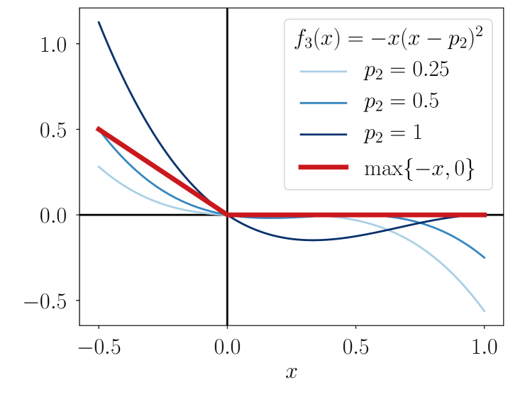
Figure A.1: Comparison of $f_{3}(x)=-x(x-p_{2})^{2}$ with the negated rectifier function $r(-x)=\max\left\{-x,0\right\}$ for different values of $p_{2}$ in the relevant interval $[-1/2,1]$ Rana (2013).

On the level of polynomials, the condition $f_{3}(x)\leq 0$ whenever $x>0$ is most important. It implies that positive eigenvalues of $X$ can never increase the value of $F_{3}(X)=\sum_{i=1}^{d}f_{3}(\lambda_{i})$. In particular, $F_{3}(X)\leq 0$ whenever $X$ is positive semidefinite – as stated in Proposition 1. The $p_{3}$-PPT condition is sound, i.e. it has no false positives.

Conversely, $f_{3}(x)>0$ for $x<0$ implies that $F_{3}(X)$ can become positive if $X$ has negative eigenvalues. Hence, the $p_{3}$-PPT condition is not vacuous. It is capable of detecting negative eigenvalues in many, but not all, unit-trace matrices $X$.

Let us now return to the (matrix-dependent) parameter choice in Eq. (17). In principle, every polynomial of the form $f_{3}^{(a)}(x)=-x(x-a)^{2}$ with $a\in\mathbb{R}$ obeys the important structure constraints (21) and therefore produces a sound test for negative eigenvalues. For fixed $X$, the associated matrix polynomial evaluates to

$$F_{3}^{(a)}(X)=-\mathrm{tr}(X^{3})+2a\mathrm{tr}(X^{2})-a^{2}\mathrm{tr}(X).$$ (24)

We can optimize this expression over the parameter $a\in\mathbb{R}$ to make the test as strong as possible. The optimal choice is $a_{\sharp}=\mathrm{tr}(X^{2})/\mathrm{tr}(X)$ and produces a matrix polynomial that obeys $F^{(a^{\sharp})}_{3}(X)\geq\max_{a\in\mathbb{R}}F_{3}^{(a)}(X)$ for $X$ fixed. If $X$ has also unit trace, the optimal parameter becomes $a_{\sharp}=p_{2}$ and produces the $p_{3}$-PPT condition (15).

This construction of PPT conditions readily extends to higher order polynomials $f_{p}(x)=a_{p}x^{p}+\cdots a_{1}x+a_{0}$. Increasing the degree $p$ produces more expressive ansatz functions that can approximate the (negated) rectifier function – and its core properties – ever more accurately. Viewed from this angle, it becomes apparent that measuring more matrix moments can produce stronger tests for detecting negative eigenvalues. However, it is not so obvious how to choose the parameters $a_{p},\ldots,a_{0}$ “optimally”, or what “optimally” actually means in this context. Some well-known polynomial approximations of the rectifier function $r(-x)$ – like Taylor expansions of $s(-x)=\ln(1+\mathrm{e}^{-x})$ (the “softplus” function) – are not well-suited for this task, because $s(-x)>0$ even for $x>0$. This in turn would imply that the associated test condition may not be sound. We believe that a thorough analysis of these questions is timely and interesting, but would go beyond the scope of this work. We intend to address it in future research.

Appendix B $p_{3}$-PPT condition for Werner States

Werner states are bipartite quantum states in a Hilbert space $\mathcal{H}_{AB}=\mathcal{H}_{A}\otimes\mathcal{H}_{B}$ with dimensions $d_{A}=d_{B}\equiv d$, defined as

$$\rho_{W}=\alpha\binom{d+1}{2}^{-1}\Pi_{+}+(1-\alpha)\binom{d}{2}^{-1}\Pi_{-}$$ (25)

with parameter $\alpha\in[0,1]$ and $\Pi_{\pm}=\frac{1}{2}\left(\mathbb{I}\pm\Pi_{12}\right)$ projectors onto symmetric $\mathcal{H}_{+}$ and anti-symmetric $\mathcal{H}_{-}$ subspaces of $\mathcal{H}=\mathcal{H}_{+}\oplus\mathcal{H}_{-}$, respectively Watrous (2018). Here, $\Pi_{12}=\sum_{i,j=1}^{d}\ket{i}\bra{j}\otimes\ket{j}\bra{i}$ is the swap operator. We note that the eigenvalues of $\rho_{W}$ are thus given as $\lambda_{+}=\alpha\binom{d+1}{2}^{-1}$ with multiplicity $\binom{d+1}{2}$ and $\lambda_{-}=(1-\alpha)\binom{d}{2}^{-1}$ with multiplicity $\binom{d}{2}$. The reduced state $\rho_{A}$ of qudit $A$ is given by $\rho_{A}=\mathrm{Tr}_{B}[\rho_{W}]=\mathbb{I}_{A}/d$.

Using furthermore that $\Pi^{T_{A}}_{\pm}=1/2(\Delta_{1}\pm(d\pm 1)\Delta_{0})$ with $\Delta_{0}=\ket{\phi_{+}}\bra{\phi_{+}}$ being a projector onto the maximally entangled state and $\Delta_{1}=\mathbb{I}-\Delta_{0}$ Watrous (2018), we find

$$\rho^{T_{A}}_{W}=\frac{2\alpha-1}{d}\Delta_{0}+\frac{1+d-2\alpha}{d}\frac{\Delta_{1}}{d^{2}-1}$$ (26)

with eigenvalues $\lambda_{0}=(2\alpha-1)/{d}$ with multiplicity 1 and $\lambda_{1}=({1+d-2\alpha})/{d(d^{2}-1)}$ with multiplicity $d^{2}-1$.

We note that, for any $d$, $\lambda_{0}<0$ for $0\leq\alpha<1/2$. Thus, using the PPT condition, we find that $\rho_{W}$ is entangled for $0\leq\alpha<1/2$. Using the explicit expression of the eigenvalues, we can furthermore determine $\mathrm{Tr}\left[(\rho^{T_{A}})^{n}\right]$ for any $n$. We find for all local dimensions $d$

$$\mathrm{Tr}\left[(\rho^{T_{A}})^{2}\right]^{2}>\mathrm{Tr}\left[(\rho^{T_{A}})^{3}\right]\quad\text{for}\quad 0\leq\alpha<\frac{1}{2}$$ (27)

Thus, for Werner states the $p_{3}$-PPT condition is equivalent to the full PPT condition. It can be furthermore shown that Werner states are separable for $\alpha\geq 1/2$ Watrous (2018). Thus, for Werner states, the $p_{3}$-PPT condition is a necessary and sufficient condition for bipartite entanglement. This also holds true for “isotropic” states of the form $\rho=\alpha\mathbbm{1}/d^{2}+(1-\alpha)|\phi_{+}\rangle\langle\phi_{+}|$, which are closely related.

We note that Werner states can have non-positive PT-moments. For local dimension $d>3$ there exists a parameter interval $\left[0,\alpha^{*}\right)$ such that the associated Werner state (25) obeys $p_{3}=\mathrm{Tr}\big{[}(\rho_{W}^{T_{A}})^{3}\big{]}<0$ for all $\alpha\in[0,\alpha^{*})$. This highlights that the logarithm of PT-moments, appearing also in the ratio $R_{3}=-\log_{2}(p_{3}/\mathrm{Tr}[\rho^{3}])$, need not be properly defined, justifying a claim from the previous subsection. It is difficult to use entropic arguments for reasoning about relations between (logarithmic) PT-moments.

Finally, as shown in Ref. Wybo et al. , we remark that $R_{3}$ is not an entanglement monotone. For separable Werner states with $1/2\leq\alpha<1/2+1/(2d)$, it holds that $0<p_{3}<\mathrm{Tr}[\rho^{3}]$. Thus, $R_{3}=-\log_{2}(p_{3}/\mathrm{Tr}[\rho^{3}])$ can be greater than zero, even for separable states. Since $R_{3}$ equals zero for all product states, it is not an entanglement monotone Horodecki et al. (2009).

Appendix C Comparison of entanglement conditions for quench dynamics

In this section, we compare the diagnostic power of the full PPT-condition, the $p_{3}$-PPT condition and a condition based on purities of nested subsystems to detect bipartite entanglement of mixed states. Specifically, given a reduced density matrix $\rho_{AB}$ in a bipartite system $AB$, we consider:

1. the PPT-condition detecting bipartite entanglement between $A$ and $B$ for a strictly positive negativity $\mathcal{N}(\rho_{AB})=\sum_{\lambda<0}|\lambda|>0$, with $\lambda$ the spectrum of $\rho_{AB}^{T_{A}}$ Horodecki et al. (2009).

2. the $p_{3}$-PPT condition detecting bipartite entanglement between $A$ and $B$ for $1-p_{3}/p_{2}^{2}>0$.

3. a condition based on the purity of nested subsystems detecting bipartite entanglement between $A$ and $B$ for $\mathrm{Tr}[\rho_{A}^{2}]<\mathrm{Tr}[\rho_{AB}^{2}]$ with $\rho_{A}=\mathrm{Tr}_{B}[\rho_{AB}]$ the reduced density matrix of subsystem $A$ Horodecki et al. (2009).

The latter ’purity’ condition was used in previous experimental works measuring the second Rényi entropy Islam et al. (2015); Kaufman et al. (2016); Linke et al. (2018); Brydges et al. (2019) to reveal bipartite entanglement of weakly mixed states.

To test these conditions, we consider here, as an example, quantum states generated via quench dynamics in interacting spin models. Specifically, we study quenches in the $XY$-model with long-range interactions, as defined in Eq. (6) of the main text, in a total system with $N=10$ spins. The initial separable product state is a Néel state $\ket{\uparrow\downarrow\uparrow\downarrow\dots}$.

As shown in Fig. C.1, the negativity (red lines) detects bipartite entanglement for all partitions sizes and all times after the quench. The $p_{3}$-PPT condition (blue lines) performs similar for the partitions considered in panel (b) and (c) and is thus able to detect bipartite entanglement for highly mixed states $\rho_{AB}$ whose purity decreases to $~{}0.3$ for the panel (b) at late times. The $p_{3}$-PPT conditions fails however to detect the entanglement for the close-to completely mixed states of small partitions $|AB|=4$ at late times, displayed in panel (a). This can be attributed to the fact that the $p_{3}$-PPT condition only relies on low order PT-moments. The purity condition (green lines) is only useful for the detection of entanglement for large partitions $AB$ with $|AB|=8$ (panel (c)). These remain weakly mixed during the entire time evolution, since the total system of $N=10$ spins is described here by a pure state.

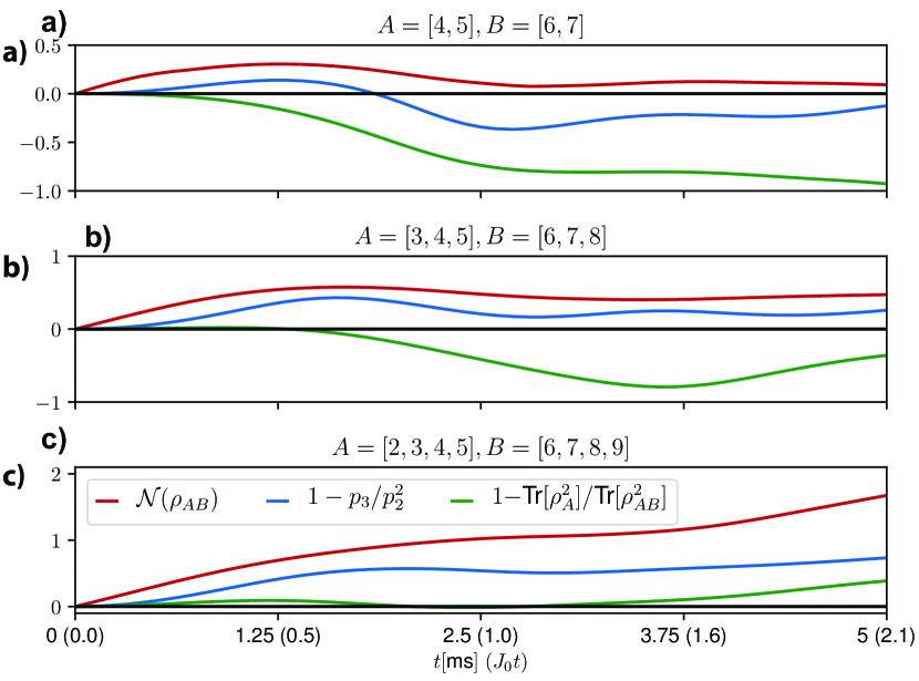
Figure C.1: Comparing conditions for bipartite entanglement between two subsystems $A$ and $B$ for states generated with quench dynamics governed by $H_{XY}$ arising from an initial Néel state in a total system with $N=10$ spins. Modeling the experiment of Ref. Brydges et al. (2019), we chose $J_{0}=420s^{-1},\alpha=1.24$, while other parameter choices lead to similar results. In all panels, and for all quantities, a strictly positive value signals bipartite entanglement.

Appendix D Error bars for PT moment predictions

Let us first review the data acquisition procedure. To obtain meaningful information about an $N$-qubit state $\rho$, we first perform a collection of random single qubit rotations: $\rho\mapsto u\rho u^{\dagger}$, where $u=u_{1}\otimes\cdots\otimes u_{N}$ and each $u_{i}$ is chosen from a unitary 3-design. Subsequently, we perform computational basis measurements and store the outcome:

$$\rho\mapsto u\rho u^{\dagger}\mapsto|k_{1},\dots,k_{N}\rangle.$$ (28)

Here, $k_{1},\ldots,k_{N}\in\left\{0,1\right\}$ denote the measurement outcomes on qubits $1,\dots,N$. As shown in Elben et al. (2019); Paini and Kalev ; Huang et al. (2020), the outcome of this measurement provides a (single-shot) estimate for the unknown state:

$$\hat{\rho}=\bigotimes_{i=1}^{N}\left[3(u_{i})^{\dagger}\ket{k_{i}}\bra{k_{i}}u_{i}-\mathbb{I}_{2}\right]$$ (29)

This tensor product is a random matrix – the unitaries $u^{(i)}$, as well as the observed outcomes $k_{i}$ are random – that produces the true underlying state in expectation:

$$\mathbb{E}\left[\hat{\rho}\right]=\rho.$$ (30)

Thus, the result of a (randomly selected) single-shot measurement provides a classical snapshot (29) that reproduces the true underlying state in expectation. This desirable feature extends to density matrices of subsystems. Let $AB\subset\left\{1,\ldots,N\right\}$ be a subset of $|AB|\leq N$ qubits and let $\rho_{AB}=\mathrm{Tr}_{\neg AB}(\rho)$ the associated reduced density matrix. Then,

$$\hat{\rho}_{AB}=\mathrm{Tr}_{\neg AB}(\hat{\rho})= \bigotimes_{i\in AB}\left[3(u_{i})^{\dagger}\ket{k_{i}}\bra{k_{i}}u_{i}-\mathbb{I}_{2}\right]$$ (31)

obeys $$\quad\mathbb{E}\left[\hat{\rho}_{AB}\right]=\rho_{AB}.$$

This feature can be used to estimate linear properties of the subsystem in question: $o=\mathrm{Tr}\left(O\rho_{AB}\right)$. Perform $M$ independent repetitions of the data acquisition procedure and use them to create a collection of (independent) snapshots $\hat{\rho}_{AB}^{(1)},\ldots,\hat{\rho}_{AB}^{(M)}$ – a “classical shadow” Huang et al. (2020) – and form the empirical average of subsystem properties:

$$\hat{o}=\tfrac{1}{M}\sum_{r=1}^{M}\mathrm{Tr}\left(O\hat{\rho}_{AB}^{(r)}\right).$$ (32)

Convergence to the target value $o=\mathbb{E}\left[\hat{o}\right]=\mathrm{Tr}(O\rho_{AB})$ is controlled by the variance. Chebyshev’s inequality asserts

$$\mathrm{Pr}\left[\left|\hat{o}-o\right|\geq\epsilon\right]\leq\frac{\mathrm{Var}\left[\hat{o}\right]}{\epsilon^{2}}=\frac{\mathrm{Var}\left[\mathrm{Tr}(O_{AB}\hat{\rho}_{AB})\right]}{M\epsilon^{2}}.$$ (33)

The remaining (single-shot) variance obeys the following useful relation.

Fact 2 (Proposition 3 in Huang et al. (2020)).

Fix a subsystem $AB$ and a linear function $\mathrm{Tr}(O\rho_{AB})$. Then, the single-shot variance associated with $\hat{\rho}_{AB}$ defined in Eq. (31) obeys

$$\mathrm{Var}\left[\mathrm{Tr}\left(O\hat{\rho}_{AB}\right)\right]\leq 2^{|AB|}\mathrm{Tr}\left(O^{2}\right).$$ (34)

This inequality is true for any underlying state $\rho$ and bounds the variance in terms of the subsystem dimension $d_{A}=2^{|AB|}$ and the Hilbert-Schmidt norm (squared) of the observable $O$. Thus, roughly $M\approx 2^{|AB|}\mathrm{Tr}(O^{2})/\epsilon^{2}$ measurement repetitions are necessary to predict $o$ up to accuracy $\epsilon$.

D.1 Predicting quadratic properties ($p_{2}$)

The formalism introduced above readily extends to predictions of higher order polynomials. The special case of quadratic functions has already been addressed in Refs. van Enk and Beenakker (2012); Elben et al. (2018); Brydges et al. (2019); Elben et al. (2019), and Ref. Huang et al. (2020) (for the present formalism). The key idea is to represent a quadratic function in $\rho$ as a linear function on the tensor product $\rho\otimes\rho$:

$$o=\mathrm{Tr}\left(O\rho_{AB}\otimes\rho_{AB}\right).$$ (35)

This function can be approximated by replacing $\rho\otimes\rho$ with a symmetric tensor product of two distinct snapshots $\hat{\rho}^{(i)},\hat{\rho}^{(j)}$ ($i\neq j$):

$$\tfrac{1}{2!} \sum_{\pi\in\mathcal{S}_{2}}\hat{\rho}_{AB}^{(\pi(i))}\otimes\hat{\rho}_{AB}^{(\pi(j))}$$

$$=\tfrac{1}{2}\left(\hat{\rho}_{AB}^{(i)}\otimes\hat{\rho}_{AB}^{(j)}+\hat{\rho}_{AB}^{(j)}\otimes\hat{\rho}_{AB}^{(i)}\right).$$ (36)

There are $\binom{M}{2}$ different ways of combining a collection of $M$ snapshots $\hat{\rho}^{(1)},\ldots,\hat{\rho}^{(M)}$ in this fashion. We can predict $o=\mathrm{Tr}(O\rho_{AB}\otimes\rho_{AB})$ by forming the empirical average over all of them:

$$\hat{o}= \binom{M}{2}^{-1}\sum_{i<j}\mathrm{Tr}\left(O\tfrac{1}{2!}\sum_{\pi\in\mathcal{S}_{2}}\hat{\rho}_{AB}^{(\pi(i))}\otimes\hat{\rho}_{AB}^{(\pi(j))}\right)$$

$$= \binom{M}{2}^{-1}\sum_{i<j}\mathrm{Tr}\left(O_{(s)}\hat{\rho}_{AB}^{(i)}\otimes\hat{\rho}_{AB}^{(j)}\right).$$ (37)

Here, we have implicitly defined the symmetrization $O_{(s)}$ of the original target function $O$. This ansatz is a special case of Hoeffding’s U-statistics estimator Hoeffding (1992). Averaging boosts convergence to the desired expectation $\mathbb{E}\left[\hat{o}\right]=o$ and the speed of convergence is controlled by the variance (33).

Restriction to subsystems is also possible. Suppose that $O$ only acts nontrivially on a subsystem $AB$ of both state copies. Then,

$$\hat{o}=\binom{M}{2}^{-1}\sum_{i<j}\mathrm{Tr}\left(O_{(s)}\hat{\rho}_{AB}^{(i)}\otimes\hat{\rho}_{AB}^{(j)}\right)$$ (38)

and the effective problem dimension becomes $d_{AB}^{2}=4^{|AB|}$. The tensor product structure (29) of the individual snapshots allows for generalizing linear variance bounds to this setting. Simply view $\hat{\rho}^{(i)}_{AB}\otimes\hat{\rho}^{(j)}_{AB}$ as a single snapshot of the quantum state $\rho_{AB}\otimes\rho_{AB}$. Fact 2 then ensures

$$\mathrm{Var}\left[\mathrm{Tr}\left(O_{(s)}\hat{\rho}_{AB}^{(i)}\otimes\hat{\rho}_{AB}^{(j)}\right)\right]\leq 4^{|AB|}\mathrm{Tr}\left(O_{(s)}^{2}\right).$$ (39)

The full variance of $\hat{o}$ is controlled in part by this relation, but also features linear variance terms (Huang et al., 2020, App. 6.A). Rather than reviewing this argument in full generality, let us focus on the task at hand: computing the variance associated with predicting the PT-moment of order two. Fix a bipartite subsystem $AB$ of interest and rewrite $p_{2}$ as

$$p_{2} =\mathrm{Tr}\left((\rho_{AB}^{(T_{A})})^{2}\right)=\mathrm{Tr}\left(\rho_{AB}^{2}\right)$$

$$=\mathrm{Tr}\left(\Pi_{AB}\rho_{AB}\otimes\rho_{AB}\right).$$ (40)

Here, $\Pi_{AB}$ denotes the swap operator that permutes the entire subsystems $AB$ within two copies of the global system. We refer to Table 1 below for a visual derivation of this well-known relation. The swap operator is symmetric under permuting tensor factors, Hermitian ($\Pi^{\dagger}_{AB}=\Pi_{AB}$) and orthogonal ($\Pi^{2}_{AB}=\mathbb{I}_{AB}$). These properties ensure that the associated general estimator (38) can be simplified considerably:

$$\hat{p}_{2}= \binom{M}{2}^{-1}\sum_{i<j}\mathrm{Tr}\left(\Pi_{AB}\hat{\rho}^{(i)}_{AB}\otimes\hat{\rho}^{(j)}_{AB}\right)$$

$$= \binom{M}{2}^{-1}\sum_{i<j}\mathrm{Tr}\left(\hat{\rho}^{(i)}_{AB}\hat{\rho}^{(j)}_{AB}\right).$$ (41)

By construction, $\mathbb{E}\left[\hat{p}_{2}\right]=p_{2}=\mathrm{Tr}(\rho^{2})$ and the speed of convergence is controlled by the variance. This variance decomposes into a linear and a quadratic part. We expand the definition of the variance:

$$\mathrm{Var}\left[\hat{p}_{2}\right]=\mathbb{E}\left[(\hat{p}_{2}-\mathbb{E}[\hat{p}_{2}])^{2}\right]=\mathbb{E}\left[\hat{p}_{2}^{2}\right]-\mathbb{E}\left[\hat{p}_{2}\right]^{2}$$ (42)

$$=\binom{M}{2}^{-2}\sum_{i<j}\sum_{k<l}\Big{(}\mathrm{Tr}\big{(}\hat{\rho}_{AB}^{(i)}\hat{\rho}_{AB}^{(j)}\big{)}\mathrm{Tr}\big{(}\hat{\rho}_{AB}^{(k)}\hat{\rho}_{AB}^{(l)}\big{)}-\mathrm{Tr}(\rho_{AB}^{2})^{2}\Big{)}.$$

The size and nature of each contribution depends on the relation between the indices $i,j,k,l$ Hoeffding (1992):

1. all indices are distinct: distinct indices label independent snapshots. In this case the expectation value factorizes completely and produces $\mathbb{E}\left[\mathrm{Tr}(\hat{\rho}_{AB}^{(i)}\hat{\rho}_{AB}^{(j)})\mathrm{Tr}(\hat{\rho}_{AB}^{(k)}\hat{\rho}_{AB}^{(l)})\right]=\mathrm{Tr}(\rho_{AB}^{2})^{2}$. This is completely offset by the subtraction of the expectation value squared. Hence, terms where all indices are distinct do not contribute to the variance.

2. exactly two indices coincide: In this case, the expectation value partly factorizes, e.g. $\mathbb{E}\left[\mathrm{Tr}(\hat{\rho}_{AB}^{(i)}\hat{\rho}_{AB}^{(j)})\mathrm{Tr}(\hat{\rho}_{AB}^{(k)}\hat{\rho}_{AB}^{(j)})\right]=\mathbb{E}\left[\mathrm{Tr}(\rho_{AB}\hat{\rho}_{AB}^{(j)})^{2}\right]$ for $i\neq k$ and $j=l$. Such index combinations produce a linear variance term $\mathrm{Var}\left[\mathrm{Tr}(O\hat{\rho})\right]$ with $O=\rho_{AB}$. The entire sum contains $\binom{M}{2}\binom{2}{1}\binom{M-2}{2-1}=\binom{M}{2}2(M-2)$ terms of this form.

3. two pairs of indices coincide: there are $\binom{M}{2}\binom{2}{2}\binom{M-2}{2-2}=\binom{M}{2}$ contributions of this form and each of them produces a quadratic variance $\mathrm{Var}\left[\mathrm{Tr}\left(O\hat{\rho}_{AB}\otimes\hat{\rho}_{AB}^{\prime}\right)\right]$ with $O=\Pi_{AB}$ (swap).

We conclude that the variance of $\hat{p}_{2}$ decomposes into linear and quadratic terms. These can be controlled via Rel. (34) and Rel. (39), respectively:

$$\mathrm{Var}\left[\hat{p}_{2}\right]= \binom{M}{2}^{-1}\left(\vphantom{\left[\hat{\rho}_{AB}^{(2)}\right]}2(M-2)\mathrm{Var}\left[\mathrm{Tr}(\rho_{AB}\hat{\rho}_{AB})\right]\right.$$

$$\qquad\qquad\left.+\mathrm{Var}\left[\mathrm{Tr}(\Pi_{AB}\hat{\rho}_{AB}^{(1)}\otimes\hat{\rho}_{AB}^{(2)})\right]\right)$$

$$\leq \frac{4(M-2)2^{|AB|}}{M(M-1)}\mathrm{Tr}\left(\rho_{AB}^{2}\right)+\frac{2\times 4^{|AB|}}{M(M-1)}\mathrm{Tr}\left(\Pi^{2}_{AB}\right)$$

$$\leq 4\left(\frac{2^{|AB|}p_{2}}{M}\right)+4\left(\frac{2^{1.5|AB|}}{M}\right)^{2}.$$ (43)

Chebyshev’s inequality (33) allows us to translate this insight into an error bound.

Lemma 2 (Error bound for estimating $p_{2}$).

Fix a subsystem $AB$ of interest and suppose that we wish to estimate $p_{2}=\mathrm{Tr}\big{(}(\rho_{AB}^{T_{A}})^{2}\big{)}$. For $\epsilon,\delta>0$, a total of

$$M\geq 8\max\left\{\frac{2^{|AB|}p_{2}}{\epsilon^{2}\delta},\frac{2^{1.5|AB|}}{\epsilon\sqrt{\delta}}\right\}$$ (44)

snapshots suffice to ensure that the estimator (41) obeys $|\hat{p}_{2}-p_{2}|\leq\epsilon$ with probability at least $1-\delta$.

It is worthwhile to briefly discuss this two-pronged error bound. Asymptotically, i.e. for $M\to\infty$, the approximation error decays at a rate proportional to $1/\sqrt{M}$. This is the expected asymptotic decay rate for an estimation procedure that relies on empirical averaging (Monte Carlo). The actual rate is also multiplicative, i.e. the approximation error is proportional to the target $p_{2}$. In the practically more relevant, non-asymptotic setting, things can look strikingly different. For small and moderate sample sizes $M$, the variance bound (43) is dominated by the next-to-leading order term ($2^{1.5|AB|}>2^{|AB|}p_{2}$, especially if $p_{2}$ is small). Lemma 2 captures this discrepancy and heralds an error decay rate proportional to $1/M$ in this regime.

Finally, we point out that the dependence on $\delta$ in Eq. (44) can be considerably improved by using median of means estimation Huang et al. (2020): split the total data into equally sized chunks, construct independent estimators and take their median. For this procedure, a sampling rate proportional to $\log(1/\delta)$ suffices. Moreover, median of means is much more robust towards outlier corruption and allows for using the same data to predict purities of many different subsystems simultaneously. This, however, comes at the price of somewhat larger constants in the error bound (44) and heralds a tradeoff. In statistical terms, median of means estimation dramatically increases confidence levels ($1-\delta$) at the cost of slightly larger error bars (confidence intervals). This tradeoff becomes advantageous when one attempts to predict very many properties from a single data set.

D.2 Predicting cubic properties ($p_{3}$ and $\mathrm{Tr}(\rho_{AB}^{3})$)

Cubic properties can be predicted in much the same fashion as quadratic properties Huang et al. (2020). Write $o=\mathrm{Tr}\left(O\rho_{AB}\otimes\rho_{AB}\otimes\rho_{AB}\right)$ and approximate $\rho\otimes\rho\otimes\rho$ by a symmetric tensor product of three distinct snapshots $\hat{\rho}_{AB}^{(i)},\hat{\rho}_{AB}^{(j)},\hat{\rho}_{AB}^{(k)}$:

$$\tfrac{1}{3!}\sum_{\pi\in\mathcal{S}_{3}}\hat{\rho}_{AB}^{(\pi(i))}\otimes\hat{\rho}_{AB}^{(\pi(j))}\otimes\hat{\rho}_{AB}^{(\pi(k))}.$$ (45)

There are $\binom{M}{3}$ different ways of combining a collection of $M$ (independent) snapshots $\hat{\rho}_{AB}^{(1)},\ldots,\hat{\rho}_{AB}^{(M)}$ in this fashion. We estimate the cubic function $o$ by averaging over all of them (U-statistics Hoeffding (1992)):

$$\hat{o}={\binom{M}{3}}^{-1}\sum_{i<j<k}\mathrm{Tr}\left(O\tfrac{1}{3!}\sum_{\pi\in\mathcal{S}_{3}}\hat{\rho}^{(\pi(i))}\otimes\hat{\rho}^{(\pi(j))}\otimes\hat{\rho}^{(\pi(k))}\right).$$ (46)

Once more, the variance controls the rate of convergence to the desired target value $\mathbb{E}\left[\hat{o}\right]=\mathrm{Tr}\left(O\rho\otimes\rho\otimes\rho\right)$. This variance decomposes into a linear, a quadratic and a cubic part. The argument is a straightforward generalization of the analysis from the previous subsection. Rather than repeating the steps in full generality, we directly focus on the 3rd order PT-moment $p_{3}$ of a subsystem $AB$:

$$p_{3}=\mathrm{Tr}\left((\rho_{AB}^{T_{A}})^{3}\right).$$ (47)

For notational simplicity, we suppress the subscript $AB$ indicating the subsystem of interest and label the shadows by lower-case indices: $\hat{\rho}^{(i)}_{AB}\mapsto\hat{\rho}_{i}$ for $i=1,\ldots,M$. Due to the cyclicity of the trace, the U-statistics estimator simplifies to

$$\binom{M}{3}\hat{p}_{3}= \sum_{i<j<k}\mathrm{Tr}\left(\tfrac{1}{3!}\sum_{\pi\in\mathcal{S}_{3}}\hat{\rho}_{\pi(i)}^{T_{A}}\hat{\rho}_{\pi(j)}^{T_{A}}\hat{\rho}_{\pi(k)}^{T_{A}}\right)$$ (48)

$$= \sum_{i<j<k}\tfrac{1}{2}\left(\mathrm{Tr}\left(\hat{\rho}_{i}^{T_{A}}\hat{\rho}_{j}^{T_{A}}\hat{\rho}_{k}^{T_{A}}\right)+\mathrm{Tr}\left(\hat{\rho}_{j}^{T_{A}}\hat{\rho}_{i}^{T_{A}}\hat{\rho}_{k}^{T_{A}}\right)\right),$$

where we have moved the normalization factor $\binom{M}{3}^{-1}$ to the left hand side in order to to increase readability. When computing the variance, we need to consider two sums over triples of distinct indices in $\left\{1,\ldots,M\right\}$. If all indices are distinct, the overall contribution vanishes. Otherwise the contribution depends on the number $c\in\left\{1,2,3\right\}$ of indices the triples have in common. The number of distinct choices for two triples with exactly $c$ integers in common is $\binom{M}{3}\binom{3}{c}\binom{M-3}{3-c}$ and we infer

$$\binom{M}{3}\mathrm{Var}\left[\hat{p}_{3}\right]$$

$$= \binom{3}{1}\binom{M-3}{2}\mathrm{Var}\left[\mathrm{Tr}\left((\rho^{T_{A}})^{2}\hat{\rho}^{T_{A}}_{1}\right)\right]$$

$$+ \binom{3}{2}\binom{M-3}{1}\mathrm{Var}\left[\mathrm{Tr}\left(\rho^{T_{A}}\tfrac{1}{2}\left(\hat{\rho}_{1}^{T_{A}}\rho_{2}^{T_{A}}+\hat{\rho}_{2}^{T_{A}}\hat{\rho}_{1}^{T_{A}}\right)\right)\right]$$

$$+ \mathrm{Var}\left[\tfrac{1}{2}\left(\mathrm{Tr}\left(\hat{\rho}_{1}^{T_{A}}\hat{\rho}_{2}^{T_{A}}\hat{\rho}_{3}^{T_{A}}\right)+\mathrm{Tr}\left(\hat{\rho}_{2}^{T_{A}}\hat{\rho}_{1}^{T_{A}}\hat{\rho}_{3}^{T_{A}}\right)\right)\right]$$

$$\leq \binom{M}{3}\left(\frac{9}{M}L+\frac{18}{M^{2}}Q+\frac{12}{M^{3}}C\right).$$ (49)

Here, $\hat{\rho}_{1},\hat{\rho}_{2},\hat{\rho}_{3}$ denote independent, random realizations of the snapshot $\hat{\rho}$ and we have introduced place-holders for linear ($L$), quadratic ($Q$) and cubic ($C$) contributions, respectively. For the task at hand, these contributions can be bounded individually and depend on the subsystem size $AB$:

1. linear contribution: set $O=(\rho^{T_{A}}_{AB})^{2}$ for notational brevity. We can use $\mathrm{Tr}(O\hat{\rho}^{T_{A}})=\mathrm{Tr}(O^{T_{A}}\hat{\rho})$ to absorb the partial transpose in the linear function. Rel. (34) then ensures

   $$L\leq 2^{|AB|}\mathrm{Tr}(\rho^{2})^{2},$$ (50)

   where we have also used $\mathrm{Tr}((O^{T_{A}})^{2})=\mathrm{Tr}(O^{2})$, as well as $\mathrm{Tr}(O^{2})=\|O\|_{2}^{2}\leq\|O\|_{1}^{2}=\mathrm{Tr}(O)^{2}$, because $O=\rho^{2}$ is psd.

2. quadratic contribution: We can bring $\tfrac{1}{2}\left(\mathrm{Tr}(\rho^{T_{A}}\hat{\rho}_{1}^{T_{A}}\hat{\rho}_{2}^{T_{A}})+\mathrm{Tr}(\rho^{T_{A}}\hat{\rho}_{2}^{T_{A}}\hat{\rho}_{1}^{T_{A}}\right)$ into the canonical form $\mathrm{Tr}\left(O\hat{\rho}_{AB}^{(1)}\otimes\hat{\rho}_{AB}^{(2)}\right)$ by introducing

   $$O=\tfrac{1}{2} \left(\Pi_{A}(\rho\otimes\mathbb{I}_{AB})\Pi_{B}\right.$$

   $$\left.+\Pi_{B}(\rho\otimes\mathbb{I}_{AB})\Pi_{A}\right).$$ (51)

   We refer to Table 1 for a visual derivation. Here, $\Pi_{A}$ and $\Pi_{B}$ are permutation operators that swap the two $A$- and $B$-systems, respectively. Rel. (39) then ensures

   $$Q\leq 2^{2|AB|}\mathrm{Tr}\left(O^{2}\right)\leq 2^{3|AB|}\mathrm{Tr}(\rho^{2}).$$ (52)

   The final estimate follows from exploiting $\Pi_{A}^{2}=\Pi_{B}^{2}=\mathbb{I}_{AB}$, as well as $\mathrm{Tr}\left(\rho^{2}\otimes\mathbb{I}_{AB}^{2}\right)=2^{|AB|}\mathrm{Tr}(\rho^{2})$.

3. cubic contribution: We can bring the cubic function $\tfrac{1}{2}\big{(}\mathrm{Tr}(\hat{\rho}^{T_{A}}_{1}\hat{\rho}^{T_{A}}_{2}\hat{\rho}^{T_{A}}_{3})+\mathrm{Tr}(\hat{\rho}^{T_{A}}_{2}\hat{\rho}^{T_{A}}_{1}\hat{\rho}^{T_{A}}_{3})\big{)}$ into the canonical form $\mathrm{Tr}\big{(}O\hat{\rho}_{1}\otimes\hat{\rho}_{2}\otimes\hat{\rho}_{3}\big{)}$ by introducing

   $$O=\tfrac{1}{2}\left(\overrightarrow{\Pi}_{A}\otimes\overleftarrow{\Pi}_{B}+\overrightarrow{\Pi}^{\dagger}_{A}\otimes\overleftarrow{\Pi}^{\dagger}_{B}\right),$$ (53)

   see Table 1 below. Here, $\overrightarrow{\Pi}_{A}$ is a cyclic permutation that exchanges all $A$-systems in a “forward” fashion ($A_{1}\mapsto A_{2}$, $A_{2}\mapsto A_{3}$, $A_{3}\mapsto A_{1}$), while $\overleftarrow{\Pi}_{B}$ is another cyclic permutation that exchanges all $B$-systems in a “backwards” fashion ($B_{3}\mapsto B_{2}$, $B_{2}\mapsto B_{1}$, $B_{1}\mapsto B_{3}$). A staightforward extension of Rel. (39) to cubic functions implies

   $$C\leq 2^{3|AB|}\mathrm{Tr}(O^{2})\leq 2^{6|AB|},$$ (54)

   because permutations are orthogonal ($\Pi\Pi^{\dagger}=\mathbb{I}$) and $\mathrm{Tr}(O^{2})$ is dominated by $\mathrm{Tr}(\mathbb{I}_{AB}\otimes\mathbb{I}_{AB}\otimes\mathbb{I}_{AB})=2^{3|AB|}$.

Inserting these bounds into the variance formula for $p_{3}$ reveals

$$\mathrm{Var}\left[\hat{p}_{3}\right]\leq \frac{9}{M}L+\frac{18}{M^{2}}Q+\frac{12}{M^{3}}C$$ (55)

$$\leq 9\frac{2^{|AB|}}{M}\mathrm{Tr}(\rho^{2})^{2}+18\frac{2^{3|AB|}}{M^{2}}\mathrm{Tr}(\rho^{2})+12\frac{2^{6|AB|}}{M^{3}}.$$

Combining this insight with Chebyshev’s inequality (33) produces a suitable error bound. Recall that $p_{2}=\mathrm{Tr}\big{(}(\rho^{T_{A}})^{2}\big{)}=\mathrm{Tr}(\rho^{2})\in[2^{-|AB|},1]$ denotes the purity of the subsystem in question.

Lemma 3 (Error bound for estimating $p_{3}$).

Fix a subsystem $AB$ of interest and suppose that we wish to estimate $p_{3}=\mathrm{Tr}\big{(}(\rho^{T_{A}})^{3}\big{)}$. For $\epsilon,\delta>0$, a total of

$$M\geq 39\max\left\{\frac{2^{|AB|}p_{2}^{2}}{\epsilon^{2}\delta},\frac{2^{1.5|AB|}p_{2}}{\epsilon\sqrt{\delta}},\frac{2^{2|AB|}}{\epsilon^{2/3}\delta^{1/3}}\right\}$$ (56)

snapshots suffice to ensure that the estimator (48) obeys $|\hat{p}_{3}-p_{3}|\leq\epsilon$ with probability at least $1-\delta$.

This bound on the sampling rate provides different error decay rates for different regimes. For $M\to\infty$, the first term in the maximum dominates and the error decays at an asymptotically unavoidable rate proportional to $1/\sqrt{M}$. Conversely, for very small sample sizes $M$, the third term dominates and conveys a much larger decay rate proportional to $1/M^{3/2}$. In the intermediate regime, the second term may dominate and lead to a inverse linear decay rate $1/M$, instead. The dependence on the error parameter $\delta$ can once more be considerably improved (from $1/\delta$ to $\log(1/\delta)$) by using median of means estimation. This refinement also allows for using the same data to predict the cubic PT-moment of very many subsystems simultaneously Huang et al. (2020).

Finally, we point out that the estimation error for $s_{3}=\|\rho\|_{3}^{3}=\mathrm{Tr}(\rho^{3})$ can be bounded in exactly the same fashion. For $\epsilon,\delta>0$, a sampling rate $M$ that obeys Rel. (56) also ensures that the U-statistics estimator U-statistics estimator

$$\hat{s}_{3}=\binom{M}{3}^{-1}\sum_{i<j<k}\tfrac{1}{2} \left(\mathrm{Tr}\left(\hat{\rho}_{i}\hat{\rho}_{j}\hat{\rho}_{k}\right)\right.$$

$$\left.\;+\mathrm{Tr}\left(\hat{\rho}_{j}\hat{\rho}_{i}\hat{\rho}_{k}\right)\right)$$ (57)

obeys $\left|\hat{s}_{3}-s_{3}\right|\leq\epsilon$ with probability $1-\delta$.

The proof is almost identical to the $p_{3}$-analysis and we leave it as an exercise for the dedicated reader.

D.3 Additional numerical simulations

Here, we complement Fig. 2 of the MT by showing in Fig. D.1 statistical errors in the estimation of $p_{2}$ and $p_{3}$ for the ground state of the transverse Ising model $H=J(\sum_{i}\sigma_{i}^{x}\sigma_{i+1}^{x}+\sigma_{i}^{z})$ at criticality. We observe the same scaling behavior as in the case of the GHZ state. For $p_{2}$ [panel a)], there are indeed two regimes with different decay rates ($1/M$ and $1/\sqrt{M}$). For $p_{3}$ [panel b)], the latter two decay rates $1/M$ and $1/\sqrt{M}$ are also clearly visible. In contrast, the early regime decay rate is not as pronounced. This is likely due to limited system sizes – $1/M^{3/2}$ does appropriately capture the decay of red dots (largest system size considered) in the top left corner, but seems to be absent in decay rates for smaller system sizes.

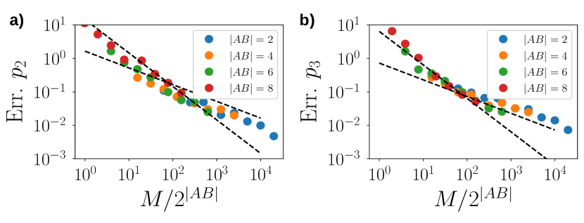
Figure D.1: Statistical errors for the ground state of the transverse field Ising model. Dashed lines represent scalings of $\propto 1/M$, and $\propto 1/\sqrt{M}$. In all cases, the number of measurements to estimate $p_{2}$ a) and $p_{3}$ b) with accuracy $~{}0.1$ is of the order of $100\times 2^{|AB|}$.

Appendix E Auxiliary results and wiring diagrams

expression	diagram representation	diagram reformulation	modified expression

Table 1: Reformulations of relevant tensor product expressions: The variance bounds in Sub. D.1 and Sub. D.2 are contingent on bringing certain expressions into canonical form, i.e. $\mathrm{Tr}\left(OX_{AB}\otimes Y_{AB}\right)$ for bilinear functions and $\mathrm{Tr}\left(O^{\prime}X_{AB}\otimes Y_{AB}\otimes Z_{AB}\right)$ for trilinear ones. This table supports visual derivations for these reformulations. Expressions of interest (very left) are first translated into wiring diagrams (center left). Subsequently, the rules of wiring calculus are used to re-arrange the diagrams (center right). Translating them into formulas (very right) produces equivalent expressions that respect the desired structure.

The arguments from the previous subsections make use of identities satisfied by traces of partial transposes of bipartite operators. Wiring diagrams – also known as tensor network diagrams – provide a useful pictorial calculus for deriving such identifies. We refer the interested reader to Refs. Landsberg (2012); Bridgeman and Chubb (2017); Kueng (2019) for a thorough introduction and content ourselves here with a concise overview that will suffice for the purposes at hand. The wiring formalism represents operators as boxes with lines emanating from them. These lines represent contra- (on the left) and co-variant indices (on the right):

$$X=\sum_{i,j}\left[X_{ij}\right]|i\rangle\!\langle j|=\leavevmode\hbox to37.97pt{\vbox to17.9pt{\text{[drawing]}}}. X i j X i j$$ (58)

Two operators $X$ and $Y$ can be multiplied to produce another operator. This corresponds to an index contraction and is represented in the following fashion:

$$XY= \sum_{i,k}(\sum_{j}\left[X\right]_{ij}\left[X\right]_{jk})|i\rangle\!\langle k|=\leavevmode\hbox to66.71pt{\vbox to17.9pt{\text{[drawing]}}}. X Y j i k X Y j i k$$ (59)

Transposition exchanges outgoing (contravariant) and incoming (covariant) indices

$$X^{T}= \sum_{i,j}\left[X\right]_{ij}|j\rangle\!\langle i|=\leavevmode\hbox to52.19pt{\vbox to21.94pt{\text{[drawing]}}}, X j i X j i$$ (60)

while the trace pairs up both indices and sums over them:

$$\mathrm{Tr}(X)= \sum_{i}\left[X\right]_{ii}=\leavevmode\hbox to36.37pt{\vbox to27.89pt{\text{[drawing]}}}=\leavevmode\hbox to50.19pt{\vbox to14.63pt{\text{[drawing]}}}. X i X X i X$$ (61)

We abbreviate this loop (contraction of leftmost and rightmost indices) by putting two circles at the end points of lines that should be contracted. This notation is not standard, but will considerably increase the readability of more complex contraction networks.

This basic formalism readily extends to tensor products if we arrange tensor product factors in parallel. For instance, a bipartite operator features two parallel lines on the left and on the right:

$$X_{AB}= X_{AB} A A B B$$ (62)

The upper lines represent the system $A$, while the lower lines represent system $B$. Two important bipartite operators are the identity $\mathbb{I}$ (do nothing) and the swap operator $\Pi$ that exchanges the systems:

$$\leavevmode\hbox to43.48pt{\vbox to21.74pt{\text{[drawing]}}}=\leavevmode\hbox to29.25pt{\vbox to15.03pt{\text{[drawing]}}}\quad\text{and}\quad\leavevmode\hbox to43.48pt{\vbox to21.74pt{\text{[drawing]}}}=\leavevmode\hbox to29.25pt{\vbox to15.03pt{\text{[drawing]}}}. \mathbb{I} \Pi \mathbb{I} \Pi$$ (63)

Rules for multiplying and contracting operators readily extend to the tensor setting. This allows us to reformulate well-known expressions pictorially. For instance,

$$\mathrm{Tr}(XY)= \leavevmode\hbox to71.53pt{\vbox to14.63pt{\text{[drawing]}}}=\leavevmode\hbox to78.65pt{\vbox to35.97pt{\text{[drawing]}}} X Y X Y X Y X Y$$ (64)

$$= \mathrm{Tr}\left(\Pi X\otimes Y\right).$$ (65)

The wiring formalism is also exceptionally well-suited to capture partial operations, like the partial transpose:

$$X_{AB}^{T_{A}}= \leavevmode\hbox to43.48pt{\vbox to29.05pt{\text{[drawing]}}}. X_{AB} X_{AB}$$ (66)

These elementary rules can be used to visually represent more complicated expressions – like a trace of multiple partial transposes. The wiring formalism provides a pictorial representation for such objects and a visual framework for modifying them. In particular, it is possible to bend, as well as unentangle, index lines and rearrange tensor factors at will. Table 1 collects several such modifications that are important for the arguments above.