Functions with average smoothness:
structure, algorithms, and learning

Abstract

We initiate a program of average smoothness analysis for efficiently learning real-valued functions on metric spaces. Rather than using the Lipschitz constant as the regularizer, we define a local slope at each point and gauge the function complexity as the average of these values. Since the mean can be dramatically smaller than the maximum, this complexity measure can yield considerably sharper generalization bounds — assuming that these admit a refinement where the Lipschitz constant is replaced by our average of local slopes.

Our first major contribution is to obtain just such distribution-sensitive bounds. This required overcoming a number of technical challenges, perhaps the most formidable of which was bounding the empirical covering numbers, which can be much worse-behaved than the ambient ones. Our combinatorial results are accompanied by efficient algorithms for smoothing the labels of the random sample, as well as guarantees that the extension from the sample to the whole space will continue to be, with high probability, smooth on average. Along the way we discover a surprisingly rich combinatorial and analytic structure in the function class we define.

1 Introduction

Smoothness is a natural measure of complexity commonly used in learning theory and statistics. Perhaps the simplest method of quantifying the smoothness of a function is via the Lipschitz seminorm. The latter has the advantage of being an analytically and algorithmically convenient, broadly applicable complexity measure, requiring only a metric space (as opposed to additional differentiable structure). In particular, the Lipschitz constant yields immediate bounds on the fat-shattering dimension (Gottlieb et al., 2014), covering numbers (Kolmogorov and Tihomirov, 1961), and sample compression (Gottlieb et al., 2018) of a function class, which in turn directly imply generalization bounds for classification and regression, and also bounds the run-time of associated learning algorithms.

The simplicity of the Lipschitz seminorm, however, has a downside: it is a worst-case measure, insensitive to the underlying distribution. As such, it can be overly pessimistic in that a single point pair can drive the Lipschitz constant of a function arbitrarily high, even if the function is nearly constant everywhere else. Intuitively, we expect the complexity of learning a function that is highly smooth, apart from low-density regions of high fluctuation, to be determined by its average — rather than worst-case — behavior. To this end, we seek a complexity measure that is resilient to local fluctuations in low-density regions. Formalizing this intuition and exploring its analytic and algorithmic ramifications is the main contribution of this paper.

Very roughly speaking, to learn an $L$-Lipschitz (in the Euclidean metric) function $f:[0,1]^{d}\to[0,1]$ at fixed precision and confidence requires on the order of $L^{d}$ examples (Wainwright, 2019), and this continues to hold in more general metric spaces (Kpotufe, 2011; Kpotufe and Dasgupta, 2012; Kpotufe and Garg, 2013; Gottlieb et al., 2017, 2014; Chaudhuri and Dasgupta, 2014). The goal of this paper is to replace the worst-case Lipschitz constant $L$ by an average one $\bar{L}$, while still obtaining bounds of the genral form $\bar{L}^{d}$. Further, we seek fully empirical generalization bounds, without making any a priori assumptions on either the target function or the distribution.

1.1 Our contributions

A detailed roadmap of our results is given in Section 2; here we only provide a brief overview. We initiate a program of average-case smoothness analysis for efficiently learning binary and real-valued functions on metric spaces. To any function $f:\Omega\to\mathbb{R}$ acting on a metric probability space $(\Omega,\rho,\mu)$, we associate a complexity measure ${\overbracket{\Lambda}}_{f}={\overbracket{\Lambda}}_{f}(\Omega,\rho,\mu)\in[0,\infty]$, which corresponds to an average slope. Our measure always satisfies ${\overbracket{\Lambda}}_{f}\leq\left\|f\right\|_{\operatorname{Lip}}$ and, as we illustrate below, the gap can be considerable. Having defined our notion of average smoothness, we show that the worst-case Lipschitz constant $L$ can essentially be replaced by its averaged variant ${\overbracket{\Lambda}}_{f}$ in the covering number bounds.

Our results are fully empirical in that we make no a priori assumptions on the target function or the sampling distribution, and only require a finite diameter and doubling dimension of the metric space. A curious and unique feature of our setting — which also presents the bulk of the technical challenges — is the fact that although our hypothesis class is fixed before observing the data, it is defined in terms of the unknown sampling distribution, and hence not explicitly known to the learner. This is in stark contrast with all previous supervised learning settings, where the function classes are fully known a priori. Having observed a sufficiently large sample allows the learner to construct an explicit hypothesis and conclude that, with high probability, it belongs to the average smoothness class (to which our generalization bounds then apply).

The statistical generalization bounds are accompanied by efficient algorithms for performing sample smoothing and a Lipschitz-type extension for label prediction on test points. The function classes we define turn out to exhibit a surprisingly rich structure, making them an object worthy of future study. See Section 2 for a comprehensive overview of our techniques and central results, along with comparisons to the current state-of-art bounds.

1.2 Related work

For the line segment metric $(\Omega,\rho)=([a,b],\left|\cdot\right|)$, the bounded variation (BV) of any $f:[a,b]\to\mathbb{R}$ with integrable derivative is given by $V_{a}^{b}(f)=\int_{a}^{b}\left|f^{\prime}(x)\right|\mathrm{d}x$; this is perhaps the most basic notion of average smoothness. BV does not require differentiability; see Appell et al. (2014) for an encyclopedic reference. Generalization bounds for BV functions may be obtained via covering numbers (Bartlett et al., 1997; Long, 2004) (the latter also gave an efficient algorithm for learning BV functions via linear programming) or the fat-shattering dimension (Anthony and Bartlett, 1999, Theorem 11.12). The aforementioned results correspond to the case of a uniformly distributed $\mu$ on $[a,b]$, and thus are not distribution-sensitive. A natural extension of BV to general measures would be to define $V_{a}^{b}(f)=\int_{a}^{b}\left|f^{\prime}(x)\right|\mathrm{d}\mu(x)$, but then the known fat-shattering and covering number estimates break down — especially if $\mu$ is not known to the learner.

Generalizing the notion of BV to higher dimensions is not nearly as straightforward. A common approach is via the Hardy-Krause variation (Appell et al., 2014; Kuipers and Niederreiter, 1974; Niederreiter and Talay, 2006). Even the two-dimensional case evades a simple characterization; counter-intuitively, Lipschitz functions $f:[0,1]^{2}\to\mathbb{R}$ may fail to have finite variation in the Hardy-Krause sense (Basu and Owen, 2016, Lemma 1). Some (rather loose) ${\sf{L}}_{1}$ covering numbers for BV functions on $[0,1]^{n}$ were obtained by Dutta and Nguyen (2018, Theorem 3.1); these are not distribution-sensitive. Generalizations of BV to metric measure spaces beyond the Euclidean are known (Ambrosio and Ghezzi, 2016); we are not aware of any covering number or combinatorial dimension estimates for these.

If one considers bracketing (rather than covering) numbers, there are known results for controlling these in terms of various measures of average smoothness. Nickl and Pötscher (2007) bound the bracketing numbers of Besov- and Sobolev-type classes. Malykhin (2010) also gave bracketing number bounds, using a different notion of smoothness: the averaged modulus of continuity developed by Sendov and Popov (1988). We note that covering numbers asymptotically always give tighter estimates than bracketing ones (Hanneke, 2018). More significantly, to our knowledge, all of the previous results bound the ambient rather than the empirical covering numbers (see Section 1.3 for definitions, and Section 3 for bounds), when it is precisely the latter that are needed for Uniform Glivenko-Cantelli laws (Giné and Zinn, 1984).

A seminal work on recovering functions with spacially inhomogeneous smoothness from noisy samples is Donoho and Johnstone (1998). More in the spirit of our program is the notion of Probabilistic Lipschitzness (Urner and Ben-David, 2013), which seeks to relax a hard Lipschitz condition on the labeling function in binary classification. The authors position it as a “data niceness” condition, analogous to that in Mammen and Tsybakov (1999). These significantly differ from our notion of average slope. Most importantly, PL and the various Tsybakov-type noise conditions are assumptions on the data-generating distribution rather then empirically computable quantities on a given sample. Our approach is fully empirical in the sense of not making a priori assumptions on the distribution or the target function. Additionally, PL is specifically designed for binary classification with deterministic labels — unlike our notion, which is applicable to any real-valued function and any conditional label distribution.

In this paper, we make systematic use of a Lipschitz-type extension (PMSE, defined in Section B) explicitly tailored to our framework. This extension is closely related to one introduced by Oberman (2008) (also relevant is Shvartsman (2017), p. 385 and p. 416, Remark 5.1).

1.3 Definitions and preliminaries

Metric probability spaces.

We assume a basic familiarity with metric measure spaces and refer the reader to a standard reference, such as Heinonen (2001). Standard set-theoretic notation is used throughout; in particular, for $f:\Omega\to\mathbb{R}$ and $A\subset\Omega$, we denote the restriction of $f$ to $A$ by $\left.f\right|_{A}$. The triple $(\Omega,\rho,\mu)$ is a metric probability space if $\mu$ is a probability measure supported on the Borel $\sigma$-algebra induced by the open sets of $\rho$. For $\Omega$-valued random variables, the notation $X\sim\mu$ means that $\mathop{\mathbb{P}}(X\in A)=\mu(A)$ for all Borel sets $A$.

Covers, packings, nets, hierarchies, partitions.

The diameter of $A\subseteq\Omega$ is the maximal interpoint distance: $\operatorname{diam}(A)=\sup_{x,x^{\prime}\in A}\rho(x,x^{\prime})$. For $t>0$ and $A,B\subseteq\Omega$, we say that $A$ is a $t$-cover of $B$ if

$$\sup_{b\in B}\inf_{a\in A}\rho(a,b)\leq t,$$

and define the $t$-covering number of $B$ to be the minimum cardinality of any $t$-cover, denoted by $\mathscr{N}(t,B,\rho)$. We say that $A\subseteq B\subseteq\Omega$ is a $t$-packing of $B$ if $\rho(a,a^{\prime})>t$ for all distinct $a,a^{\prime}\in A$. Finally, $A$ is a $t$-net of $B$ if it is simultaneously a $t$-cover and a $t$-packing. A family of sets $H_{t^{0}}\subseteq H_{t^{-1}}\subseteq\ldots\subseteq H_{t^{-m}}$ is a hierarchy for the set $H_{t^{-m}}$ if each $H_{t^{-i}}$ ($i<m$) is a $t^{-i}$-net of $H_{t^{-(i+1)}}$, where we have assumed that $H_{t^{-m}}$ have diameter $1$ and so $H_{1}$ contains a single point.

We denote by $B(x,r)=\left\{x^{\prime}\in\Omega:\rho(x,x^{\prime})\leq r\right\}$ the (closed) $r$-ball about $x$. If there is a $D<\infty$ such that every $r$-ball in $\Omega$ is contained in the union of some $D$ $r/2$-balls, the metric space $(\Omega,\rho)$ is said to be doubling. Its doubling dimension is defined as $\operatorname{ddim}(\Omega)=\operatorname{ddim}(\Omega,\rho)=:\log_{2}D^{*}$, where $D^{*}$ is the smallest $D$ verifying the doubling property. It is well-known (Krauthgamer and Lee, 2004; Gottlieb et al., 2016) that

$$\mathscr{N}(t,\Omega,\rho)\leq\left(\frac{2\operatorname{diam}(\Omega)}{t}\right)^{\operatorname{ddim}(\Omega)},\qquad t>0,$$ (1)

which will be referred to as the covering property of doubling spaces. The packing property of doubling spaces asserts an analogous packing number bound, up to constants in the exponent. A hierarchy for any $n$-point $\Omega$ set can be constructed in time $2^{O(\operatorname{ddim}(\Omega))}\min\{\log n,\log\Delta\}$, where $\Delta$ is the aspect ratio (minimal interpoint distance) of $\Omega$ (Krauthgamer and Lee, 2004; Har-Peled and Mendel, 2006; Cole and Gottlieb, 2006).

To any finite $V\subseteq\Omega$ we associate the map $\varphi_{V}:\Omega\to V$ taking each $x\in\Omega$ to its nearest neighbor in $V$, with ties broken arbitrarily (say, via some fixed ordering on $\Omega$). The collection of sets $\left\{\varphi_{V}^{-1}(v):v\in V\right\}$ is said to comprise the Voronoi partition of $\Omega$ induced by $V$. If $V$ happens to be a $t$-net of $\Omega$, then

$$\rho(x,\varphi_{V}(x))\leq t,\qquad x\in\Omega.$$ (2)

Indices, norms.

We write $[n]:=\left\{1,\ldots,n\right\}$ and use the shorthand $z_{[n]}:=(z_{1},\ldots,z_{n})$ for sequences. For any metric probability space $(\Omega,\rho,\mu)$, $p\geq 1$, and any $f:\Omega\to\mathbb{R}$, we define the norm $\|f\|_{{\sf{L}}_{p}(\Omega,\rho,\mu)}^{p}=\mathop{\mathbb{E}}_{X\sim\mu}[|f(X)|^{p}]=\int_{\Omega}|f(x)|^{p}\mathrm{d}\mu(x)$.

This work assumes a single fixed metric probability space $(\Omega,\rho,\mu)$; this will be termed the ambient space. Several derived metric probability spaces $(\Omega^{\prime},\rho^{\prime},\mu^{\prime})$ will be considered, which will all be induced subspaces of $(\Omega,\rho)$ in the sense that $\Omega^{\prime}\subseteq\Omega$ and $\rho^{\prime}=\left.\rho\right|_{\Omega^{\prime}\times\Omega^{\prime}}$. To lighten the notation, we will often suppress the common metric $\rho$ and use the shorthand $\|\cdot\|_{{\sf{L}}_{p}(\mu^{\prime})}:=\|\cdot\|_{{\sf{L}}_{p}(\Omega^{\prime},\rho,\mu^{\prime})}$. For any $f,g:\Omega\to\mathbb{R}$ and any induced subspace $(\Omega^{\prime},\rho)$ of $\Omega$ with measure $\mu^{\prime}$, we use the shorthand

$$\|f-g\|_{{\sf{L}}_{p}(\mu^{\prime})}:=\left\|\left.f\right|_{\Omega^{\prime}}-\left.g\right|_{\Omega^{\prime}}\right\|_{{\sf{L}}_{p}(\mu^{\prime})}=\|\left.f\right|_{\Omega^{\prime}}-\left.g\right|_{\Omega^{\prime}}\|_{{\sf{L}}_{p}(\Omega^{\prime},\rho,\mu^{\prime})}.$$ (3)

In particular, sampling $\Omega_{n}:=X_{[n]}=(X_{1},\ldots,X_{n})\sim\mu^{n}$ induces the empirical space $(\Omega_{n},\rho,\mu_{n})$ with the norm $\|\cdot\|_{{\sf{L}}_{p}(\mu_{n})}$, where $\mu_{n}$ is the empirical measure on $\Omega_{n}$, formally given by $\mu_{n}(x)=n^{-1}\sum_{i=1}^{n}\boldsymbol{{1}}[X_{i}=x]$. The $\ell_{\infty}$ norm $\|f\|_{\infty}=\sup_{x\in\Omega}\left|f(x)\right|$ is measure-independent and dominates all of the measure-induced norms:

$$\|f-g\|_{{\sf{L}}_{p}(\mu^{\prime})}\leq\|f-g\|_{\infty},\qquad p\geq 1.$$

The Lipschitz seminorm $\left\|f\right\|_{\operatorname{Lip}}$ is the smallest $L\in[0,\infty]$ satisfying $\left|f(x)-f(x^{\prime})\right|\leq L\rho(x,x^{\prime})$ for all $x,x^{\prime}\in\Omega$.

Strong and weak mean.

We define the weak mean of a non-negative random variable $Z$ by

$$\mathop{\mathbb{W}}[Z]=\sup_{t>0}t\mathop{\mathbb{P}}(Z\geq t).$$ (4)

In contrast, the strong mean is just the usual expectation $\mathop{\mathbb{E}}[Z]$. By Markov’s inequality, we always have $\mathop{\mathbb{W}}[Z]\leq\mathop{\mathbb{E}}[Z]$; further, the latter might be infinite while the former is finite. A partial reverse inequality for finite measure spaces is given in Lemma 22.

Local and average slope.

For $f:\Omega\to\mathbb{R}$, we define the slope of $f$ at $x\in\Omega$ with respect to an $A\subseteq\Omega$ as

$$\Lambda_{f}(x,A):=\sup_{x^{\prime}\in A\setminus\left\{x\right\}}\frac{|f(x)-f(x^{\prime})|}{\rho(x,x^{\prime})}.$$ (5)

Thus,

$$\left\|f\right\|_{\operatorname{Lip}}=\sup_{x\in\Omega}\Lambda_{f}(x,\Omega).$$ (6)

We will define two notions of average slope: strong and weak, corresponding, respectively, to the strong and weak ${\sf{L}}_{1}$ norms of the random variable $\Lambda_{f}(X)$, where $X\sim\mu$. The two averages are defined, respectively, as

$${\overbracket{\Lambda}}_{f}(\mu,\Omega) := \mathop{\mathbb{E}}_{X\sim\mu}\left[\Lambda_{f}(X,\Omega)\right]=\|\Lambda_{f}(\cdot,\Omega)\|_{{\sf{L}}_{1}(\mu)},$$ (7)

$${\widetilde{\Lambda}}_{f}(\mu,\Omega) := \mathop{\mathbb{W}}_{X\sim\mu}\left[\Lambda_{f}(X,\Omega)\right]=\sup_{t>0}t\mu(M_{f}(t)),$$ (8)

where $M_{f}(t)$ is the $t$-level set, a central object in this paper:

$$M_{f}(t):=\left\{x\in\Omega:\Lambda_{f}(x,\Omega)\geq t\right\}.$$ (9)

The strong-weak mean inequality above implies that

$${\widetilde{\Lambda}}_{f}(\mu,\Omega)\leq{\overbracket{\Lambda}}_{f}(\mu,\Omega)\leq\left\|f\right\|_{\operatorname{Lip}}$$ (10)

always holds (the second inequality is obvious); further, ${\overbracket{\Lambda}}_{f}(\mu,\Omega)$ might be infinite while ${\widetilde{\Lambda}}_{f}(\mu,\Omega)$ is finite (as demonstrated by the step function on $[0,1]$ with the uniform measure, see Section F). Since the above definitions were stated for any metric probability space, $\Lambda_{f}(x,\Omega_{n})$, ${\overbracket{\Lambda}}_{f}(\mu_{n},\Omega_{n})$, and ${\widetilde{\Lambda}}_{f}(\mu_{n},\Omega_{n})$ are well-defined as well. (To appreciate the subtle choice of our definitions, note that some intuitively appealing variants irreparably fail, as discussed in Section F.)

The collection of all $[0,1]$-valued $L$-Lipschitz functions on $\Omega$, as well as its strong and weak mean-slope counterparts are denoted, respectively, by

$$\operatorname{Lip}_{L}(\Omega,\rho) = \left\{f\in[0,1]^{\Omega};~{}\left\|f\right\|_{\operatorname{Lip}}\leq L\right\},$$ (11)

$${\overbracket{\operatorname{Lip}}}_{L}(\Omega,\rho,\mu) = \left\{f\in[0,1]^{\Omega};~{}{\overbracket{\Lambda}}_{f}(\mu,\Omega)\leq L\right\},$$ (12)

$${\widetilde{\operatorname{Lip}}}_{L}(\Omega,\rho,\mu) = \left\{f\in[0,1]^{\Omega};~{}{\widetilde{\Lambda}}_{f}(\mu,\Omega)\leq L\right\}.$$ (13)

It follows from (10) that $\operatorname{Lip}_{L}(\Omega,\rho,\mu)\subset{\overbracket{\operatorname{Lip}}}_{L}(\Omega,\rho,\mu)\subset{\widetilde{\operatorname{Lip}}}_{L}(\Omega,\rho,\mu)$, where all containments are, in general, strict, and

$$\mu(M_{f}(L/t))\leq t,\qquad t>0$$ (14)

holds for all $f\in{\widetilde{\operatorname{Lip}}}_{L}(\Omega,\rho,\mu)$. For most of this paper, we shall be interested in the larger latter class, but occasional results for ${\overbracket{\operatorname{Lip}}}_{L}(\Omega,\rho,\mu)$ will be presented, when of independent interest.

Remark: Observe that the classes ${\overbracket{\operatorname{Lip}}}$ and ${\widetilde{\operatorname{Lip}}}$ are defined in terms of the unknown sampling distribution $\mu$. Given full knowledge of a function $f:\Omega\to\mathbb{R}$, a learner can verify that $f\in\operatorname{Lip}_{L}$ but, absent full knowledge of $\mu$, it is impossible to know for certain whether $f\in{\widetilde{\operatorname{Lip}}}_{L}$ (or $f\in{\overbracket{\operatorname{Lip}}}_{L}$). As increasingly larger samples are observed, the learner will be able to assert the latter inclusions with increasing confidence.

Empirical and true risk.

For any probability measure $\nu$ on $\Omega\times[0,1]$, we associate to any measurable $f:\Omega\to\mathbb{R}$ its risk $R(f;\nu):=\mathop{\mathbb{E}}_{(X,Y)\sim\nu}|f(X)-Y|$. In the special case of the empirical measure $\nu_{n}$ induced by a sample $(X_{i},Y_{i})_{i\in[n]}\sim\nu^{n}$, $R(f;\nu_{n})$ is the empirical risk. For regression with real-valued $f$, this is the ${\sf{L}}_{1}$-risk; for classification with $\left\{0,1\right\}$-valued $f$, this is the $0$-$1$ error. (See Mohri et al. (2012) for a standard reference.)

Miscellanea.

Additional standard inequalities and notations are deferred to Section A in the Appendix.

2 Main results and roadmap

This section assumes a familiarity with the terminology and notation defined in Section 1.3.

Combinatorial structure.

Our point of departure is Theorem 1, which bounds the ${\sf{L}}_{2}(\mu)$ (ambient) covering numbers of the function class ${\widetilde{\operatorname{Lip}}}_{L}(\Omega,\rho,\mu)$ — and, a fortiori, of ${\overbracket{\operatorname{Lip}}}_{L}(\Omega,\rho,\mu)$ [defined in (12, 13)] — in terms of the average slope $L$, $\operatorname{diam}(\Omega)$, and $\operatorname{ddim}(\Omega)$. Crucially, there is no dependence on the Lipschitz constant $\left\|\cdot\right\|_{\operatorname{Lip}}$. At scale $t$, Theorem 1 gives a bound of roughly

$$\left({L}/{t}\right)^{\tilde{O}(\operatorname{ddim})}$$ (15)

instead of the previous state-of-the art bound of $({\left\|\cdot\right\|_{\operatorname{Lip}}}/{t})^{\tilde{O}(\operatorname{ddim})}$. The improvement can be dramatic, as the worst-case may be significantly (even infinitely) larger than the mean (6).

This simple result appears to be novel and interesting in its own right, but is insufficient to guarantee generalization bounds (via a Uniform Glivenko-Cantelli law), since the latter require control over the empirical (i.e., ${\sf{L}}_{2}(\mu_{n})$) covering numbers. Bounding these proved to be a formidable challenge. The calculation in Theorem 4 reduces this problem to the one of bounding the empirical measure of the level set, $\mu_{n}(M_{f}(\ell))$, uniformly over all the functions in our class. We make the perhaps surprising discovery that (i) uniform control over the $\mu_{n}(M_{f}(\ell))$ is possible for the sub-class of functions free of certain local defects (Lemma 5) and (ii) any $f\in{\widetilde{\operatorname{Lip}}}_{L}(\Omega,\rho,\mu)$ is approximable in $\ell_{\infty}$ by a defect-free function (Lemma 6); see the beginning of Section 4 for some discussion and intuition. Together, these enable us to overcome the central challenge of controlling the empirical covering numbers (Theorem 3), yielding a bound comparable to (15). The implied generalization bounds (Section D) enjoy a dependence on $\sqrt{L}/n^{1/8d}$, while all previously known generalization results for classification and regression feature a dependence on $\left\|\cdot\right\|_{\operatorname{Lip}}$ (Tsybakov, 2004; Wainwright, 2019; Gottlieb et al., 2017).

Optimization and learning.

From the perspective of supervised learning theory, our statistical bounds imply a non-trivial algorithmic problem: Given a labeled sample, produce a hypothesis whose true risk does not significantly exceed its empirical risk (with high probability). These notions are briefly defined in Section 1.3 and discussed in more detail in Section D.2. In light of the aforementioned generalization bounds, the learning procedure may be recast as follows: The learner is given a “complexity budget” $L>0$. Given a labeled sample, $(X_{i},Y_{i})\in\Omega\times[0,1]$, $i\in[n]$, the learner seeks to fit to the data some function with average slope not exceeding $L$, while minimizing the empirical risk. The latter is induced by either the $0$-$1$ loss (classification) or the ${\sf{L}}_{1}$ loss (regression). Approximation algorithms for this problem are presented in Section 5. Briefly, we cast the regression problem as an optimization problem amenable to the mixed packing-covering framework of Koufogiannakis and Young (2014), and further improve the algorithmic run-time by reducing the number of constraints in the program (Section 5.1). Interestingly, the classification problem admits an efficient bi-criteria approximation when casting the “smoothness budget” in terms of the weak mean, but we were unable to find an efficient solution for the strong mean, and provide some indication that this may in fact be a hard problem (Section 5.2).

Adversarial extension.

Having solved the learning problem, we have obtained an approximate minimizer of the empirical risk, but this does not immediately imply a bound on the true risk. To obtain such a bound, we demonstrate that with high probability, average smoothness under the empirical measure $\mu_{n}$ translates to average smoothness under the true sampling measure $\mu$, from which a bound on true risk follows.

To this end, we define the following adversarial extension problem: An adversary draws $n$ points $\Omega_{n}\subset\Omega$ from $\mu$ and labels them with $y\in[0,1]$. This induces an average slope ${\overbracket{\Lambda}}_{y}$ (or ${\widetilde{\Lambda}}_{y}$) under the empirical measure $\mu_{n}$. The adversary’s goal is to force any extension of $y$ from $\Omega_{n}$ to all of $\Omega$ to have a significantly larger average slope under the true measure $\mu$. In the case of regression, we show that if the learner is willing to tolerate a small distortion of $y$ under ${\sf{L}}_{1}(\mu_{n})$, it is possible to guarantee an at-most constant factor increase in both ${\overbracket{\Lambda}}$ and ${\widetilde{\Lambda}}$ with high probability (Section 6). In the case of classification, we show how to achieve an most $2^{O(\operatorname{ddim})}\operatorname{polylog}(n)$ factor increase (with high probability), without incurring any distortion (Section 7).

3 Covering numbers

Our covering-numbers results will be stated for ${\widetilde{\operatorname{Lip}}}_{L}$. It follows from (10) that these results hold verbatim for ${\overbracket{\operatorname{Lip}}}_{L}$ as well. (These function classes are defined in (11, 12, 13)).

3.1 Ambient covering numbers

Our empirical covering-numbers results build upon the following simpler result for the ambient covering numbers:

Theorem 1 (Ambient ${\sf{L}}_{2}$ Covering Numbers).

For $L,t>0$,

$$\log\mathscr{N}(t,{\widetilde{\operatorname{Lip}}}_{L}(\Omega,\rho,\mu),{\sf{L}}_{2}(\mu)) \leq \mathscr{N}(t^{3}/(64L),\Omega,\rho)\log(16/t).$$

In particular, for doubling spaces with $\operatorname{diam}(\Omega)\leq 1$, we have

$$\log\mathscr{N}(t,{\widetilde{\operatorname{Lip}}}_{L}(\Omega,\rho,\mu),{\sf{L}}_{2}(\mu)) \leq \left(\frac{128L}{t^{3}}\right)^{\operatorname{ddim}(\Omega)}\log\frac{16}{t}.$$

The proof of Theorem 1 will be based upon following result:

Lemma 2 (Gottlieb et al. (2017), Lemma 5.2).

For $L,t>0$,

$$\log\mathscr{N}(t,\operatorname{Lip}_{L}(\Omega,\rho),\ell_{\infty}) \leq \mathscr{N}(t/(8L),\Omega,\rho)\log(8/t).$$

In particular, for doubling spaces with $\operatorname{diam}(\Omega)=1$, we have

$$\log\mathscr{N}(t,\operatorname{Lip}_{L}(\Omega,\rho),\ell_{\infty}) \leq \left(\frac{16L}{t}\right)^{\operatorname{ddim}(\Omega)}\log\frac{8}{t}.$$

Proof of Theorem 1.

Recall the definition of the level set $M_{f}(\cdot)$ in (9). By (14), we have $\mu(M_{f}(L/t))\leq t$ for any $f\in{\widetilde{\operatorname{Lip}}}_{L}(\Omega,\rho,\mu)$ and $t>0$, and by construction, $\Lambda_{f}(x,\Omega)\leq L/t$ for all $x\in M^{\prime}_{f}(L/t):=\Omega\setminus M_{f}(L/t)$. Thus, for all $f\in{\widetilde{\operatorname{Lip}}}_{L}(\Omega,\rho,\mu)$, we have

$$\left.f\right|_{M^{\prime}_{f}(L/t)}\in\operatorname{Lip}_{L/t}(M^{\prime}_{f}(L/t),\rho).$$ (16)

Let $\hat{F}$ be a $t/2$-cover of $\operatorname{Lip}_{4L/t^{2}}(\Omega,\rho)$ under $\ell_{\infty}$. We claim that $\hat{F}$ is a $t$-cover of ${\widetilde{\operatorname{Lip}}}_{L}(\Omega,\rho,\mu)$ under ${\sf{L}}_{2}(\Omega,\rho,\mu)$. Indeed, choose an $f\in{\widetilde{\operatorname{Lip}}}_{L}(\Omega,\rho,\mu)$. It follows from (16) that

$$\left.f\right|_{M^{\prime}_{f}(4L/t^{2})}\in\operatorname{Lip}_{4L/t^{2}}(M^{\prime}_{f}(4L/t^{2}),\rho).$$ (17)

Via the McShane-Whitney Lipschitz extension (McShane, 1934; Whitney, 1934), there is an $\tilde{f}\in\operatorname{Lip}_{4L/t^{2}}(\Omega,\rho)$ coinciding with $f$ on $M^{\prime}_{f}(4L/t^{2})$. Since $\hat{F}$ is a $t/2$-cover, there is an $\hat{f}\in\hat{F}$ such that $\|\tilde{f}-\hat{f}\|_{{\sf{L}}_{2}(\mu)}\leq\|\tilde{f}-\hat{f}\|_{\infty}\leq t/2$. Therefore

$$\|f-\hat{f}\|_{{\sf{L}}_{2}(\mu)} \leq \|f-\tilde{f}\|_{{\sf{L}}_{2}(\mu)}+\|\tilde{f}-\hat{f}\|_{{\sf{L}}_{2}(\mu)}$$

$$= \left(\int_{\Omega}(f(x)-\tilde{f}(x))^{2}\mathrm{d}\mu(x)\right)^{1/2}+\|\tilde{f}-\hat{f}\|_{{\sf{L}}_{2}(\mu)}$$

$$= \left(\int_{M_{f}(4L/t^{2})}(f(x)-\tilde{f}(x))^{2}\mathrm{d}\mu(x)\right)^{1/2}+\|\tilde{f}-\hat{f}\|_{{\sf{L}}_{2}(\mu)}$$

$$\leq \left(\int_{M_{f}(4L/t^{2})}1^{2}\mathrm{d}\mu(x)\right)^{1/2}+\|\tilde{f}-\hat{f}\|_{{\sf{L}}_{2}(\mu)}$$

$$\leq t/2+t/2=t.$$

The claim follows from Lemma 2, which bounds the size of (a minimal) $\hat{F}$. ∎

3.2 Empirical covering numbers

The main result of this section is a bound on the empirical covering numbers. To avoid trivialities, we state our asymptotic bounds in $n$ under the assumption that $\operatorname{ddim}(\Omega),L\geq 1$.

Theorem 3 (Empirical ${\sf{L}}_{2}$ Covering Numbers).

Let $(\Omega,\rho,\mu)$ be a doubling metric measure space (the ambient space) with $\operatorname{diam}(\Omega)\leq 1$ and $(\Omega_{n},\rho,\mu_{n})$ its empirical realization.

Then, for constant $\delta>0$ and $L,\operatorname{ddim}(\Omega)\geq 1$, we have that

$$\log\mathscr{N}((\alpha+1)\varepsilon_{0},{\widetilde{\operatorname{Lip}}}_{L}(\Omega,\rho,\mu),{\sf{L}}_{2}(\mu_{n})) \leq \left(\frac{L}{\alpha^{3}\varepsilon_{0}^{3}}\right)^{\operatorname{ddim}(\Omega)}\log\frac{1}{\alpha\varepsilon_{0}},\qquad\alpha>0$$

holds with probability at least $1-2\delta$, where $\varepsilon_{0}\leq C_{\delta}\sqrt{L}n^{-\ifrac{1}{8d}}$ and $C_{\delta}>0$ is a universal constant.

The proof will be given below, and follows directly from Theorem 1 and the following result:

Theorem 4 (Preserving distances between ${\sf{L}}_{2}(\mu)$ and ${\sf{L}}_{2}(\mu_{n})$).

Let $(\Omega,\rho,\mu)$ be a doubling metric measure space (the ambient space) with $\operatorname{diam}(\Omega)\leq 1$ and $(\Omega_{n},\rho,\mu_{n})$ its empirical realization. Then, with probability at least $1-2\delta$, we have that all $f,g\in{\widetilde{\operatorname{Lip}}}_{L}(\Omega,\rho,\mu)$ satisfy

$$\|f-g\|_{{\sf{L}}_{2}(\mu_{n})} \leq 6\|f-g\|_{{\sf{L}}_{2}(\mu)}$$

$$+ 25n^{-\ifrac{1}{4d}}+15\sqrt{L}n^{-\ifrac{1}{8d}}+(6+2^{d/4})n^{-\ifrac{1}{8}}+\left(\frac{162}{n}\log\frac{2}{\delta}\right)^{\ifrac{1}{4}},$$

where $d=\operatorname{ddim}(\Omega)$ and we adhere to the notational convention in (3).

Proof.

Let $r,t,\eta>0$ be parameters to be chosen later. Our first step is to approximate the function class ${\widetilde{\operatorname{Lip}}}_{L}(\Omega,\rho,\mu)$ by its “$\eta$-smoothed” version

$${{\widetilde{\operatorname{Lip}}}_{L}}^{\eta}(\Omega,\rho,\mu):=\left\{f^{\eta}:f\in{\widetilde{\operatorname{Lip}}}_{L}(\Omega,\rho,\mu)\right\}\subseteq{\widetilde{\operatorname{Lip}}}_{L}(\Omega,\rho,\mu),$$

where $f^{\eta}$ is the function constructed in Lemma 6, when the latter is invoked with the parameter $\ell=L/t$. In particular, $\|f-f^{\eta}\|_{\infty}\leq 4\eta$ and $\Lambda_{f^{\eta}}(x,\Omega)\leq\Lambda_{f}(x,\Omega)$ for all $x\in\Omega$. Thus, for $f,g\in{\widetilde{\operatorname{Lip}}}_{L}(\Omega,\rho,\mu)$,

$$\|f-g\|_{{\sf{L}}_{2}(\mu_{n})} \leq \|f-f^{\eta}\|_{\infty}+\|g-g^{\eta}\|_{\infty}+\|f^{\eta}-g^{\eta}\|_{{\sf{L}}_{2}(\mu_{n})}$$ (18)

$$\leq 8\eta+\|f^{\eta}-g^{\eta}\|_{{\sf{L}}_{2}(\mu_{n})},$$

and so it will suffice to bound the latter.

Let $V\subset\Omega$ be an $r$-net of $(\Omega,\rho)$; by the doubling property (1),

$$|V|\leq(2/r)^{\operatorname{ddim}(\Omega)}.$$ (19)

The net $V$ induces the Voronoi partition $\Omega=\bigcup_{v\in V}W(v)$, such that for each cell $W(v)$ we have $x\in W(v)\implies\rho(x,v)\leq r$, as well as the measure under $\mu$, denoted by $\pi(v):=\mu(W(v))$. Together, these induce the finite metric measure space $(V,\rho,\pi)$. The map $\varphi_{V}:\Omega\to V$ takes each $x\in\Omega$ with its Voronoi cell; thus, $\varphi_{V}^{-1}(\varphi_{V}(x))=W(v)$ for all $x\in W(v)$.

The proof proceeds in several steps, in which always $f,g\in{{\widetilde{\operatorname{Lip}}}_{L}}^{\eta}(\Omega,\rho,\mu)$ and the notational convention in (3) is used. Define $M_{f}(L/t),M_{g}(L/t)\subset\Omega$ as in (9). As in the proof of Theorem 1, we have that $f$ is $L/t$-Lipschitz on $M^{\prime}_{f}(L/t):=\Omega\setminus M_{f}(L/t)$, with extension $\tilde{f}\in\operatorname{Lip}_{L/t}(\Omega,\rho)$. Define $\tilde{g}\in\operatorname{Lip}_{L/t}(\Omega,\rho)$ analogously, as extending $\left.g\right|_{M^{\prime}_{g}(L/t)}\in\operatorname{Lip}_{L/t}(M^{\prime}_{g}(L/t),\rho)$.

Comparing the norms $\|f-g\|_{{\sf{L}}_{2}(\mu_{n})}^{2}=\frac{1}{n}\sum_{i=1}^{n}(f(X_{i})-g(X_{i}))^{2}$ and $\|\tilde{f}-\tilde{g}\|_{{\sf{L}}_{2}(\pi)}^{2}=\sum_{v\in V}(\tilde{f}(v)-\tilde{g}(v))^{2}\pi(v)$.

We begin by invoking (48):

$$\|f-g\|_{{\sf{L}}_{2}(\mu_{n})}^{2}\leq 3\|\tilde{f}-\tilde{g}\|_{{\sf{L}}_{2}(\mu_{n})}^{2}+3\|f-\tilde{f}\|_{{\sf{L}}_{2}(\mu_{n})}^{2}+3\|g-\tilde{g}\|_{{\sf{L}}_{2}(\mu_{n})}^{2}.$$ (20)

The second and third terms in the bound (20) are bounded identically:

$$\|f-\tilde{f}\|_{{\sf{L}}_{2}(\mu_{n})}^{2} = \frac{1}{n}\sum_{i=1}^{n}(f(X_{i})-\tilde{f}(X_{i}))^{2}$$ (21)

$$\leq \frac{1}{n}\sum_{i:X_{i}\in M_{f}(L/t)}1\;=\;\mu_{n}(M_{f}(L/t)).$$

To estimate the first term in the bound (20), recall that $\tilde{f}$ is $L/t$-Lipschitz on $\Omega$ and $\rho(x,\varphi_{V}(x))\leq r$ (and the same holds for $\tilde{g}$), whence

$$|\tilde{f}(X_{i})-\tilde{g}(X_{i})| \leq |\tilde{f}(X_{i})-\tilde{f}(\varphi_{V}(X_{i}))|+|\tilde{g}(X_{i})-\tilde{g}(\varphi_{V}(X_{i}))|+|\tilde{f}(\varphi_{V}(X_{i}))-\tilde{g}(\varphi_{V}(X_{i}))|$$

$$\leq |\tilde{f}(\varphi_{V}(X_{i}))-\tilde{g}(\varphi_{V}(X_{i}))|+2Lr/t.$$

Using $(a+b)^{2}\leq 2a^{2}+2b^{2}$, this yields

$$\|\tilde{f}-\tilde{g}\|_{{\sf{L}}_{2}(\mu_{n})}^{2} = \frac{1}{n}\sum_{i=1}^{n}(\tilde{f}(X_{i})-\tilde{g}(X_{i}))^{2}$$

$$\leq \frac{2}{n}\sum_{i=1}^{n}(\tilde{f}(\varphi_{V}(X_{i}))-\tilde{g}(\varphi_{V}(X_{i})))^{2}+8(Lr/t)^{2}$$

$$= 2\sum_{v\in V}(\tilde{f}(v)-\tilde{g}(v))^{2}\mu_{n}(W(v))+8(Lr/t)^{2}$$

$$= 2\|\tilde{f}-\tilde{g}\|_{{\sf{L}}_{2}(\pi_{n})}^{2}+8(Lr/t)^{2},$$

where $\pi_{n}$ is the measure on $V$ given by $\pi_{n}(v)=\mu_{n}(W(v))$. Observe that

$$\left|\|\tilde{f}-\tilde{g}\|_{{\sf{L}}_{2}(\pi)}^{2}-\|\tilde{f}-\tilde{g}\|_{{\sf{L}}_{2}(\pi_{n})}^{2}\right| \leq \sum_{v\in V}(\tilde{f}(v)-\tilde{g}(v))^{2}|\pi(v)-\pi_{n}(v)|$$

$$\leq \sum_{v\in V}|\pi(v)-\pi_{n}(v)|=\|\pi-\pi_{n}\|_{1}.$$

A bound on $\|\pi-\pi_{n}\|_{1}$ is provided by (52): with probability at least $1-\delta$,

$$\|\pi-\pi_{n}\|_{1}\leq\sqrt{\frac{|V|}{n}}+\sqrt{\frac{2}{n}\log\frac{2}{\delta}}\leq\sqrt{\frac{(2/r)^{\operatorname{ddim}(\Omega)}}{n}}+\sqrt{\frac{2}{n}\log\frac{2}{\delta}}.$$

To bound $\mu_{n}(M_{f}(L/t))$ in (21), we invoke Corollary 7: with probability at least $1-\delta$,

$$\sup\left\{\mu_{n}(M_{f}(L/t)):f\in{{\widetilde{\operatorname{Lip}}}_{L}}^{\eta}(\Omega,\rho,\mu)\right\}\leq 24t+\frac{1}{2}\sqrt{\frac{(2L/\eta t)^{\operatorname{ddim}(\Omega)}}{n}}+\frac{1}{2}\sqrt{\frac{2}{n}\log\frac{2}{\delta}}.$$

These calculations culminate in the bound

$$\|f-g\|_{{\sf{L}}_{2}(\mu_{n})}^{2} \leq 6\|\tilde{f}-\tilde{g}\|_{{\sf{L}}_{2}(\pi)}^{2}+24(Lr/t)^{2}+144t$$

$$+ 6\sqrt{\frac{(2/r)^{\operatorname{ddim}(\Omega)}}{n}}+9\sqrt{\frac{2}{n}\log\frac{2}{\delta}}+3\sqrt{\frac{(2L/\eta t)^{\operatorname{ddim}(\Omega)}}{n}}.$$

Comparing the norms $\|\tilde{f}-\tilde{g}\|_{{\sf{L}}_{2}(\pi)}^{2}$ and $\|f-g\|_{{\sf{L}}_{2}(\mu)}^{2}$ .

Since $\tilde{f}$ is $L/t$-Lipschitz and $\operatorname{diam}(W(v))\leq r$, we have $\tilde{f}(W(v))\subseteq f(v)\pm Lr/t$, and analogously for $\tilde{g}$. It follows that

$$|\tilde{f}(v)-\tilde{g}(v)| \leq |\tilde{f}(x)-\tilde{g}(x)|+2Lr/t,\qquad x\in W(v)$$ (23)

and hence

$$(\tilde{f}(v)-\tilde{g}(v))^{2} \leq 2(\tilde{f}(x)-\tilde{g}(x))^{2}+8(Lr/t)^{2},\qquad x\in W(v).$$ (24)

Integrating,

$$\|\tilde{f}-\tilde{g}\|_{{\sf{L}}_{2}(\pi)}^{2}=\sum_{v\in V}(\tilde{f}(v)-\tilde{g}(v))^{2}\pi(v) = \sum_{v\in V}\int_{W(v)}(\tilde{f}(v)-\tilde{g}(v))^{2}\mathrm{d}\mu(x)$$

$$\leq \sum_{v\in V}\int_{W(v)}[2(\tilde{f}(x)-\tilde{g}(x))^{2}+8(Lr/t)^{2}]\mathrm{d}\mu(x)$$

$$= 2\|\tilde{f}-\tilde{g}\|_{{\sf{L}}_{2}(\mu)}^{2}+8(Lr/t)^{2}.$$

Using (48) and the triangle inequality, we have

$$\|\tilde{f}-\tilde{g}\|_{{\sf{L}}_{2}(\mu)}^{2} \leq 3\|f-g\|_{{\sf{L}}_{2}(\mu)}^{2}+3\|f-\tilde{f}\|_{{\sf{L}}_{2}(\mu)}^{2}+3\|g-\tilde{g}\|_{{\sf{L}}_{2}(\mu)}^{2}$$

$$\leq 3\|f-g\|_{{\sf{L}}_{2}(\mu)}^{2}+6t$$

(since each of $\|f-\tilde{f}\|_{{\sf{L}}_{2}(\mu)},\|g-\tilde{g}\|_{{\sf{L}}_{2}(\mu)}$ is at most $\sqrt{t}$).

Combining these yields

$$\|\tilde{f}-\tilde{g}\|_{{\sf{L}}_{2}(\pi)}^{2} \leq 6\|f-g\|_{{\sf{L}}_{2}(\mu)}^{2}+12t+8(Lr/t)^{2}.$$ (25)

Finishing up.

Combining (3.2) and (25) yields

$$\|f-g\|_{{\sf{L}}_{2}(\mu_{n})}^{2} \leq 36\|f-g\|_{{\sf{L}}_{2}(\mu)}^{2}+72(Lr/t)^{2}+216t$$

$$+ 6\sqrt{\frac{(2/r)^{\operatorname{ddim}(\Omega)}}{n}}+9\sqrt{\frac{2}{n}\log\frac{2}{\delta}}+3\sqrt{\frac{(2L/\eta t)^{\operatorname{ddim}(\Omega)}}{n}}.$$

Choosing $r,t,\eta$.

Putting $d=\operatorname{ddim}(\Omega)$, we choose $r=n^{-\ifrac{1}{2d}}$, $t=Ln^{-\ifrac{1}{4d}}$, and $\eta=2n^{-\ifrac{1}{4d}}$. For this choice,

$$\|f-g\|_{{\sf{L}}_{2}(\mu_{n})}^{2} \leq 36\|f-g\|_{{\sf{L}}_{2}(\mu)}^{2}+72n^{-{1}/{2d}}+216Ln^{-{1}/{4d}}$$

$$+ 2^{d/2}\cdot 6n^{-{1}/{4}}+9\sqrt{\frac{2}{n}\log\frac{2}{\delta}}+3\left(n^{1/4d}\right)^{d/2}n^{-\ifrac{3}{8}}.$$

Applying the inequality $\sqrt{a+b}\leq\sqrt{a}+\sqrt{b}$ to (3.2) proves the claim. ∎

Proof of Theorem 3.

Let $\varepsilon_{+}$ be the additive term in the bound in Theorem 4:

$$\varepsilon_{+}=25n^{-\ifrac{1}{4d}}+15\sqrt{L}n^{-\ifrac{1}{8d}}+(6+2^{d/4})n^{-\ifrac{1}{8}}+\left(\frac{162}{n}\log\frac{2}{\delta}\right)^{\ifrac{1}{4}}.$$ (27)

Since for fixed $\delta>0$ and $d,L\geq 1$ the dominant term in (28) is $15\sqrt{L}n^{-\ifrac{1}{8d}}$, and so there is a $C=C_{\delta}<0$ such that

$$\varepsilon_{+}\leq C_{\delta}\sqrt{L}n^{-\ifrac{1}{8d}}=:\varepsilon_{0}.$$ (28)

Now Theorem 4 implies that any $\varepsilon$-cover of ${\widetilde{\operatorname{Lip}}}_{L}(\Omega,\rho,\mu)$ under ${\sf{L}}_{2}(\mu)$ also provides a $(6\varepsilon+\varepsilon_{0})$-cover under ${\sf{L}}_{2}(\mu_{n})$. Equivalently, an $\alpha\varepsilon_{0}/6$-cover of the former yields an $(\alpha+1)\varepsilon_{0}$-cover of the latter, for $\alpha>0$. Hence,

$$\log\mathscr{N}((\alpha+1)\varepsilon_{0},{\widetilde{\operatorname{Lip}}}_{L}(\Omega,\rho,\mu),{\sf{L}}_{2}(\mu_{n})) \leq \log\mathscr{N}(\alpha\varepsilon_{0}/6,{\widetilde{\operatorname{Lip}}}_{L}(\Omega,\rho,\mu),{\sf{L}}_{2}(\mu))$$

$$\leq \left(\frac{cL}{\alpha^{3}\varepsilon_{0}^{3}}\right)^{\operatorname{ddim}(\Omega)}\log\frac{1}{\alpha\varepsilon_{0}},$$

where $c>0$ is a universal constant.

∎

4 Defect free functions

This section presents results that were invoked in the proofs in Section 3. It constitutes the core of the analytic and combinatorial structure we discovered in the very general setting of real-valued functions on metric spaces. Such a function may fail to be on-average smooth for two “moral” reasons: due to “large jumps” or “small jumps”. The former is witnessed by two nearby points $x,x^{\prime}$ for which $|f(x)-f(x^{\prime})|$ is large — say, $1$. The latter is witnessed by two nearby (say, $\varepsilon$-close) points $x,x^{\prime}$ for which $\varepsilon\ll|f(x)-f(x^{\prime})|\leq T(\varepsilon)\ll 1$ — say, $T(\varepsilon)=\sqrt{\varepsilon}$. It turns out that the large jumps do not present a problem for the combinatorial structure we seek in Lemma 5, which forms the basis for Corollary 7, the latter a crucial component in the empirical covering number bound, Theorem 4. Rather, it is the small jumps — which we formalize as defects below — that present an obstruction. Fortunately, as we show in Lemma 6, any bounded real-valued function on a doubling metric space admits a defect-free approximation under $\ell_{\infty}$.

4.1 Definition and structure

For a given $f:\Omega\to\mathbb{R}$, $\ell>0$, and $x,y\in\Omega$, we say that $y$ is an $\ell$-slope witness for $x$ (w.r.t. $f$) if ${\left|f(x)-f(y)\right|}/{\rho(x,y)}\geq\ell$. For $\eta,\ell>0$ and $c\geq 1$, we say that an $x\in\Omega$ is an $(\eta,\ell,c)$-defect of $f$ if:

1. $\Lambda_{f}(x)\geq\ell$

2. Every $\ell/c$-slope witness $y$ of $x$ verifies $\left|f(x)-f(y)\right|\leq\eta$.

Define $\Xi_{f}(\eta,\ell,c)\subseteq\Omega$ to be the set of all $(\eta,\ell,c)$-defects of $f$. Note that $\Xi_{f}(\eta,\ell,c)\subseteq\Xi_{f}(\eta,\ell,c^{\prime})$ whenever $c^{\prime}\leq c$. For $\eta,\ell>0$, $c\geq 1$ define $\mathcal{G}(\eta,\ell,c)$ to be the collection of all $f:\Omega\to[0,1]$ such that $f$ does not have any $(\eta,\ell,c)$-defects.

Lemma 5 (Combinatorial structure of defect-free functions).

For every $\eta,\ell>0$, $c\geq 1$ there is a partition $\Pi=\left\{B_{1},\ldots,B_{N}\right\}$ of $\Omega$ of size $N\leq(2\ell/\eta)^{\operatorname{ddim}(\Omega)}$ such that for each $f\in\mathcal{G}(\eta,\ell,c)$, we have

$$M_{f}(\ell)\subseteq U_{f}\subseteq M_{f}(\ell/4c),$$ (29)

where $M_{f}(\cdot)$ is the level set defined in (9) and

$$U_{f}:=\bigcup\left\{B\in\Pi:B\cap M_{f}\neq\emptyset\right\}.$$ (30)

Proof.

Let $\Pi$ be the Voronoi partition induced by an $\eta/\ell$-net of $\Omega$. Then the claimed bound on $|\Pi|$ holds by (1) and the first inclusion in (29) is obvious by construction; it only remains to show that $U_{f}\subseteq M_{f}(\ell/4c)$.

Choose any $u\in U_{f}$. Since $\Pi$ is a net, there is some $x\in M_{f}(\ell)$ for which $\rho(x,u)\leq{\eta}/{\ell}$. Since $f$ has no $(\eta,\ell,c)$-defects and $\Lambda_{f}(x)\geq\ell$, there must be some ${\ell}/{c}$-slope witness $y\in\Omega$ of $x$ for which $\left|f(x)-f(y)\right|>\eta$. Invoking (49), we have ${\left|f(u)-f(x)\right|}\vee{\left|f(u)-f(y)\right|}\geq\left|f(x)-f(y)\right|/2>\eta/2$. We consider the two cases:

1. $\rho(x,y)\leq{\eta}/{\ell}$

2. $\rho(x,y)>{\eta}/{\ell}$.

In the first case, the triangle inequality implies that ${\rho(u,x)}\vee{\rho(u,y)}\leq{2\eta}/{\ell}$, and hence

$$\Lambda_{f}(u)\geq{\frac{\left|f(u)-f(x)\right|}{\rho(u,x)}}\vee{\frac{\left|f(u)-f(y)\right|}{\rho(u,y)}}\geq\frac{\eta/2}{2\eta/\ell}=\frac{\ell}{4}\geq\frac{\ell}{4c}\implies u\in M_{f}(\ell/4c).$$

For the second case, if $\left|f(u)-f(x)\right|\geq\eta/2$, the proof is the same as in the first case. Otherwise, $\left|f(u)-f(y)\right|\geq\left|f(x)-f(y)\right|/2$ and so

$$\frac{\left|f(u)-f(y)\right|}{\rho(u,y)}\geq\frac{\left|f(x)-f(y)\right|}{2\rho(u,y)}\geq\frac{\left|f(x)-f(y)\right|}{2\cdot 2\rho(x,y)}\geq\frac{\ell}{4c}\implies u\in M_{f}(\ell/4c),$$

where the second inequality is a result of applying the triangle inequality to the fact that $\rho(u,x)<\rho(x,y)$. ∎

4.2 Repairing defects

The main result of this section is that the problematic “small jumps” alluded to in the beginning of Section 4 can be smoothed out via an $\ell_{\infty}$ approximation.

Lemma 6 (Defect repair).

For each $\eta,\ell>0$ and $f:\Omega\to[0,1]$, there is an $\bar{f}\in\mathcal{G}(\eta,\ell,c=6)$ such that $\|f-\bar{f}\|_{\infty}\leq 4\eta$ and

$$\Lambda_{\bar{f}}(x,\Omega)\leq\Lambda_{f}(x,\Omega),\qquad x\in\Omega.$$ (31)

Proof.

We will prove the equivalent claim that $\bar{f}\in\mathcal{G}(\eta/2,\ell,c=6)$ and $\|f-\bar{f}\|_{\infty}\leq 2\eta$. We begin by constructing $\bar{f}$. Let $M_{f}(\ell)$ be as defined in (9) and $V$ be a ${\eta/\ell}$-net of this set. Partition $V=V_{0}\cup V_{1}$, where $V_{0}$ is “smooth,”

$$V_{0}:=\left\{v\in V:B(v,{\eta/\ell})\nsubseteq\Xi_{f}(\eta,\ell,1)\right\},$$

and $V_{1}$ is “rough,”

$$V_{1}:=\left\{v\in V:B(v,{\eta/\ell})\subseteq\Xi_{f}(\eta,\ell,1)\right\}.$$

Define

$$A_{f}:=\bigcup_{v_{1}\in V_{1}}B(v_{1},{\eta/\ell})\setminus\left(\bigcup_{v_{0}\in V_{0}}B(v_{0},{\eta/\ell})\cup V\right).$$

In words, $A_{f}$ consists of the entirely defective (or “rough”) balls without their center-points or their intersections with smooth balls. Define $\bar{f}$ as the PMSE extension of $f$ from $\Omega\setminus A_{f}$ to $\Omega$, as in Definition B.1. Having constructed the $\bar{f}$, we proceed to verify its properties.

Proof that (31) holds.

This is an immediate consequence of Theorem 20.

Proof that $\|f-\bar{f}\|_{\infty}\leq 2\eta$.

Since PMSE is an extension, we need only establish $\left|f(x)-\bar{f}(x)\right|\leq 2\eta$ for $x\in A_{f}$. For any such $x$, the definition of $A_{f}$ implies the existence of some $v_{1}\in V_{1}$ for which $\rho(x,v_{1})\leq\eta/\ell$. Since $\left|f(x)-\bar{f}(x)\right|\leq\left|f(v_{1})-f(x)\right|+\left|\bar{f}(x)-f(v_{1})\right|$, it is sufficient to bound each term separately by $\eta$.

To bound the first term, assume, for a contradiction, that $\left|f(v_{1})-f(x)\right|>\eta$. Then $\frac{\left|f(v_{1})-f(x)\right|}{\rho(v_{1},x)}>\frac{\eta}{\eta/\ell}=\ell$, contradicting the defectiveness of $v_{1}$.

To bound the second term, again assume for a contradiction that $\bar{f}(x)-f(v_{1})>\eta$; the case $f(v_{1})-\bar{f}(x)>\eta$ is handled analogously. Our assumption implies $\Lambda_{\bar{f}}(x)\geq\frac{\bar{f}(x)-\bar{f}(v_{1})}{\rho(x,v_{1})}\geq\ell$. By properties (i) and (v) of Corollary 21, there is an $x^{\prime}\in\Omega\setminus A_{f}$ for which $\Lambda_{\bar{f}}(x)=\frac{\bar{f}(x^{\prime})-\bar{f}(x)}{\rho(x^{\prime},x)}\geq\ell$ and $\bar{f}(x^{\prime})\geq\bar{f}(x)$. Invoking (51), we have $\frac{f(x^{\prime})-f(v_{1})}{\rho(x^{\prime},v_{1})}\geq\ell$. Additionally, we have $\bar{f}(x^{\prime})-\bar{f}(v_{1})>\bar{f}(x)-\bar{f}(v_{1})>\eta$, again contradicting the defectiveness of $v_{1}$.

Proof that $\bar{f}\in\mathcal{G}(\eta/2,\ell,6)$.

A statement equivalent to $\bar{f}\in\mathcal{G}(\eta/2,\ell,6)$ is that $\Xi_{\bar{f}}(\eta/2,\ell,6)=\emptyset$. Let us define the sets

$$E_{1} := \bigcup_{v_{0}\in V_{0}}B(v,{\eta/\ell}),$$

$$E_{2} := A_{f}\cup V_{1},$$

$$E_{3} := \Omega\setminus M_{f}(\ell),$$

which are, by construction, a (not necessarily disjoint) cover of $\Omega$. Hence, it suffices to show that $\Xi_{\bar{f}}(\eta/2,\ell,6)\cap E_{i}=\emptyset$ for $i\in[3]$.

Let $x\in E_{3}$. By Theorem 20, $\Lambda_{\bar{f}}(x,\Omega)\leq\Lambda_{f}(x,\Omega)$. Since $x\notin M_{f}(\ell)$, we have that $\Lambda_{\bar{f}}(x)<\ell$, implying that $x$ is not $(\eta/2,\ell,c)$-defect for any $c\geq 1$ with respect to $\bar{f}$.

Let $x\in E_{1}$. Then there is a $v_{0}\in V_{0}$ such that $\rho(x,v_{0})\leq\eta/\ell$. Being in $V_{0}$ implies that $v_{0}$ has some $\ell$-slope witness $v_{0}^{\prime}\in E_{1}$ such that $\left|f(v_{0})-f(v_{0}^{\prime})\right|>\eta$. This implies by (49) that ${\left|\bar{f}(x)-\bar{f}(v_{0})\right|}\vee{\left|\bar{f}(x)-\bar{f}(v_{0}^{\prime})\right|}>\left|f(v_{0})-f(v_{0}^{\prime})\right|/2>\eta/2$, since $f$ and $\bar{f}$ must agree on $v_{0}$ and $v_{0}^{\prime}$. The triangle inequality yields a slope of at least $\ell/4$ witnessed by at least one of $\left\{v_{0},v_{0}^{\prime}\right\}$.

Let $x\in E_{2}$. Then there is a $v_{1}\in V_{1}\subseteq\Xi_{f}(\eta,\ell,1)$ for which $\rho(x,v_{1})\leq\eta/\ell$. By Remark 1, the maximal slope at $x$ is achieved at the two distinct points $u^{*}$ and $v^{*}$ by which it is determined. Suppose ${\rho(x,u^{*})}\vee{\rho(x,v^{*})}>\eta/2\ell$. If $\Lambda_{f}(x)\geq\ell$ and one of $\left\{u^{*},v^{*}\right\}$ — say, $u^{*}$ — satisfies the inequality then:

$$\left|f(x)-f(u^{*})\right|\geq\ell\rho(x,u^{*})>\ell\cdot\frac{\eta}{2\ell}=\frac{\eta}{2}.$$

This contradicts the second condition for an $(\eta/2,\ell,c)$-defect. Otherwise, ${\rho(x,u^{*})}\vee{\rho(x,v^{*})}\leq\eta/2\ell$. Since $V$ is an $\eta/\ell$-net, it is not possible that both $u^{*},v^{*}\in V$. Therefore (without loss of generality) $u^{*}\in E_{1}\cup E_{3}$. If $u^{*}\in E_{3}$, it follows from property (ii) in Corollary 21 that

$$\Lambda_{\bar{f}}(x,\Omega)\leq\Lambda_{\bar{f}}(u^{*},\Omega)\leq\Lambda_{f}(u^{*},\Omega)<\ell,$$

which implies that $x\notin\Xi_{\bar{f}}(\eta/2,\ell,c)$ for any $c\geq 1$. If $u^{*}\in E_{1}$ then there is some $v_{0}\in V_{0}$ for which $\rho(u^{*},v_{0})\leq\eta/\ell$. Since $\Lambda_{f}(v_{0})>\ell$ and $v_{0}\notin\Xi_{f}(\eta,\ell,1)$, it must have some witness $v_{0}^{\prime}$ such that $\left|f(v_{0})-f(v_{0}^{\prime})\right|>\eta$ and the slope between them is at least $\ell$. Similarly to previous arguments, ${\left|\bar{f}(x)-\bar{f}(v_{0})\right|}\vee{\left|\bar{f}(x)-\bar{f}(v_{0}^{\prime})\right|}>\left|f(v_{0})-f(v_{0}^{\prime})\right|/2\geq\eta/2$. In either case, applying the triangle inequality yields a slope of at least $\ell/6$ witnessed by at least one of $\left\{v_{0},v_{0}^{\prime}\right\}$, which shows that $x\notin\Xi_{\bar{f}}(\eta/2,\ell,6)$.

∎

The culmination of this section is the following crucial uniform convergence result invoked in the course of proving Theorem 4:

Corollary 7.

Let $f^{\eta}$ be the function constructed from $f$ as in Lemma 6, when the latter is invoked with the parameter $\ell=L/t$, and let

$${{\widetilde{\operatorname{Lip}}}_{L}}^{\eta}(\Omega,\rho,\mu):=\left\{f^{\eta}:f\in{\widetilde{\operatorname{Lip}}}_{L}(\Omega,\rho,\mu)\right\}\subseteq{\widetilde{\operatorname{Lip}}}_{L}(\Omega,\rho,\mu).$$

Then, with probability at least $1-\delta$, we have

$$\sup\left\{\mu_{n}(M_{f}(L/t)):f\in{{\widetilde{\operatorname{Lip}}}_{L}}^{\eta}(\Omega,\rho,\mu)\right\} \leq 24t+\frac{1}{2}\sqrt{\frac{(2L/\eta t)^{\operatorname{ddim}(\Omega)}}{n}}+\frac{1}{2}\sqrt{\frac{2}{n}\log\frac{2}{\delta}},$$

where $\mu_{n}$ is the empirical measure induced by $\mu$.

Proof.

Let $\Pi$ be as in Lemma 5. For each $f\in{{\widetilde{\operatorname{Lip}}}_{L}}^{\eta}(\Omega,\rho,\mu)$, let $U_{f}$ be as defined in (30). Then, invoking the inclusion in (29) and recalling that $\mu(M_{f}(L/t))\leq t$ for all $f\in{\widetilde{\operatorname{Lip}}}_{L}(\Omega,\rho,\mu)$ and $t>0$ (and that Lemma 6 sets $c=6$),

$$\sup_{f}\mu_{n}(M_{f}(L/t)) \leq \sup_{f}\mu_{n}(U_{f})$$

$$= \sup_{f}\left[\mu_{n}(U_{f})-\mu(U_{f})\right]+\mu(U_{f})$$

$$\leq \sup_{f}\left(\mu_{n}(U_{f})-\mu(U_{f})\right)+\sup_{f}\mu(U_{f})$$

$$\leq \sup_{U\subseteq\Pi}\left(\mu_{n}(U)-\mu(U)\right)+\sup_{f}\mu(M_{f}(L/4ct))$$

$$\leq \sup_{U\subseteq\Pi}\left(\mu_{n}(U)-\mu(U)\right)+24t$$

$$= \frac{1}{2}\sum_{B\in\Pi}|\mu(B)-\mu_{n}(B)|+24t,$$

where the last step used the variational characterization of the total variation distance. The latter is bounded as in (52), completing the proof.

∎

5 Learning algorithms: training

We consider two learning problems — classification and regression — in a unified agnostic setting (Mohri et al., 2012). In each case, the learner receives a labeled sample, $(X_{i},Y_{i})_{i\in[n]}$, where $X_{i}\in\Omega$ and $Y_{i}\in\left\{0,1\right\}$ for classification or $Y_{i}\in[0,1]$ for regression. The learner then selects a hypothesis $f\in{\widetilde{\operatorname{Lip}}}_{L}(\Omega,\rho,\mu)$, where $L$ is fixed a priori. Finally, given a test point $x^{\prime}\in\Omega$, the learner’s predicted label is either $f(x^{\prime})\in[0,1]$ (regression) or ${\boldsymbol{{1}}[{f(x^{\prime})}>1/2]}\in\left\{0,1\right\}$ (classification); this is elaborated in greater detail in Section D.2. Computational considerations, as well as the learner’s inherent uncertainty regarding whether $f\in{\widetilde{\operatorname{Lip}}}_{L}(\Omega,\rho,\mu)$ (see below), will lead us to consider relaxed versions of the learning problem, where the “complexity budget” will increase from $L$ to $O(L)$ for regression and $O(L\cdot\operatorname{polylog}n)$ for classification.

As described in Section 1.3, the sample is drawn from the joint measure $\nu$ over $\Omega\times[0,1]$ — whose first marginal, by definition, necessarily coincides with $\mu$ — and, once drawn, induces the empirical measure $\nu_{n}$. The empirical (respectively, true) risk of $f:\Omega\to\mathbb{R}$ is the expected value of $|f(X)-Y|$ under $\nu$ (respectively, $\nu_{n}$); these are denoted by $R(f;\nu)$ and $R(f;\nu_{n})$. The learner seeks to minimize $R(f;\nu)$ but can only directly access $R(f;\nu_{n})$; hence, an optimization algorithm will seek to minimize the latter, while a generalization bound will provide a high-confidence bound on the former.

Our learning problem presents a novel challenge, not typically encountered in the classic supervised learning setting. Namely, ensuring that the learner’s hypothesis belongs to ${\widetilde{\operatorname{Lip}}}_{L}(\Omega,\rho,\mu)$ (or ${\overbracket{\operatorname{Lip}}}_{L}(\Omega,\rho,\mu)$) is non-trivial, and is certainly not guaranteed “by construction”. Indeed, let us break down the learning process into its basic stages. The training stage, which may be called smoothing or denoising (or yet regularization), involves solving the following optimization problem: Choose a hypothesis $f$ that stays within the “smoothness budget” and achieves a low $R(f;\nu_{n})$. Algorithmically, this is done by computing an $\hat{f}:\Omega_{n}\to[0,1]$, where $\Omega_{n}=(X_{i})_{i\in[n]}$ and $\hat{f}(X_{i})$ is a “smoothed” version of the $Y_{i}$, achieving a desired average empirical slope ${\widetilde{\Lambda}}_{\hat{f}}(\mu_{n},\Omega_{n})$ (or ${\overbracket{\Lambda}}_{\hat{f}}(\mu_{n},\Omega_{n})$). The function $\hat{f}$ is then extended via (a variant of) PMSE from $\Omega_{n}$ to all of $\Omega$. The novel challenge is to ensure that ${\widetilde{\Lambda}}_{\hat{f}}(\mu,\Omega)$ (respectively, ${\overbracket{\Lambda}}_{\hat{f}}(\mu,\Omega)$) does not much exceed its empirical version. We term this problem adversarial extension and address it in Sections 6 and 7.

The results for regression are conceptually simpler and are presented first; those for classification follow. Throughout this section, we assume $\operatorname{diam}(\Omega)\leq 1$ and $d:=\operatorname{ddim}(\Omega)<\infty$.

5.1 Regression

Theorem 8 (Training and generalization for regression, strong mean.).

Let $\nu$ be some distribution on $\Omega\times[0,1]$, and $S_{n}=(X_{i},Y_{i})_{i\in[n]}\sim\nu^{n}$ be a set sampled i.i.d. from $\nu$. Denote by $\hat{f}\in{\overbracket{\operatorname{Lip}}}_{L}(\Omega_{n},\rho,\mu_{n})$ the minimizer of $R(\cdot;\nu_{n})$. Then there is an efficient learning algorithm $\mathcal{A}$ that constructs a hypothesis $f=\mathcal{A}(S_{n})$ such that such that for any given $L>0$, $0<\varepsilon,\delta<1$ and $c<1$:

1. With probability at least $1-\exp\left({-n(\varepsilon/8)^{d+1}+d\ln{(8/\varepsilon)}}\right)-3\delta$,

   $$R(f;\nu)\leq(1+c)R(\hat{f};\nu_{n})+O\left(\varepsilon L+\frac{C_{\delta}\sqrt{L}}{n^{1/8d}}\right)+\frac{C_{\delta}^{-d/2}\sqrt{2}}{n^{5/16}}+3\sqrt{\frac{\log(2/\delta)}{2n}},$$

2. $f(x)$ can be evaluated at each $x\in\Omega$ in time $O(n^{2})$ after a one-time “smoothing” computation of $\min\{2^{O(d)}(n/c^{2})\log\Delta,O((n/c)^{2}\log n)\}$ where $\Delta=\min_{x\neq x^{\prime}\in x_{[n]}}\rho(x,x^{\prime})$,

where $C_{\delta}$ is a constant depending only on $\delta$.

Proof.

The smoothing algorithm described in Lemma 9 constructs an approximate minimizer $\tilde{f}\in{\overbracket{\operatorname{Lip}}}_{O(1)L}(\Omega_{n},\rho,\mu_{n})$ of $R(\cdot;\nu_{n})$ and the “adversarial extension” algorithm in Lemma 13 provides an extension $f$ of $\tilde{f}$ from $\Omega_{n}$ to $\Omega$ that, with high probability, belongs to ${\overbracket{\operatorname{Lip}}}_{O(1)L}(\Omega,\rho,\mu)$ and increases the empirical risk by at most an additive $O(\varepsilon L)$. The bound in (a) is then a direct application of (65).

∎

Lemma 9 (Smoothing for regression, strong mean).

Let $(\Omega,\rho)$ be a metric space with $\operatorname{diam}(\Omega)\leq 1$ and $\operatorname{ddim}(\Omega)<\infty$. Suppose that $(x,y)=(x_{[n]},y_{[n]})\in(\Omega^{n},\mathbb{R}^{n})$ and $L>0$ are given, and denote

$$A(f;x,y,L) := \{\|f-y\|_{{\sf{L}}_{1}(\mu_{n})}:\>f\in{\overbracket{\operatorname{Lip}}}_{L}(x_{[n]},\rho,\mu_{n})\},$$ (32)

where $\mu_{n}$ is the counting measure on $x_{[n]}$.

Then a $(1+c)$-approximate minimizer $\hat{f}\in{\overbracket{\operatorname{Lip}}}_{L}(x_{[n]},\rho,\mu_{n})$ of $A(\cdot;x,y,L)$ can be computed in time

$$\min\{2^{O(\operatorname{ddim}(\Omega))}(n/c^{2})\log\Delta~{},~{}O((n/c)^{2}\log n)\}.$$

Proof.

We cast the optimization problem as a linear program over the variables $L_{i},w_{i},z_{i}$:

$$\begin{array}[]{lll}\textrm{Minimize}&W=\sum_{i\in[n]}w_{i}&\\ \textrm{subject to}&\sum_{i\in[n]}L_{i}\leq L&\\ &w_{i}\geq|z_{i}-y_{i}|&\forall i\in[n]\\ &|z_{i}-z_{j}|\leq L_{i}\rho(x_{i},x_{j})&\forall i,j\in[n]\\ &0\leq w_{i},z_{i}\leq 1&\forall i\in[n].\end{array}$$

A linear program in $O(n)$ variables and constraints can be solved in time $\tilde{O}(n^{\omega})$ (Cohen et al., 2019), where $\omega$ is the best exponent for matrix inversion, currently $\omega\approx 2.37$.

First runtime improvement.

To improve on the runtime, we will utilize the packing-covering framework of Koufogiannakis and Young (2014). For a constraint matrix of at most $m$ rows and columns with all non-negative entries and at most $\zeta$ non-zero entries, the algorithm computes in time $O((m/c^{2})\log\zeta+\zeta)$ a $(1+c)$-approximate solution satisfying all constraints. A difficulty in utilizing this framework is that our constraint matrix has negative entries; in particular, each constraint of the form

$$|z_{i}-z_{j}| \leq L_{i}\cdot\rho(x_{i},x_{j})$$

reduces to solving two constraints of the form

$$z_{i}-z_{j} \leq L_{i}\cdot\rho(x_{i},x_{j})$$

$$z_{j}-z_{i} \leq L_{i}\cdot\rho(x_{i},x_{j}).$$

To address this, we introduce dummy variables $\tilde{z}_{i}$ satisfying $z_{i}+\tilde{z}_{i}=1$. Then the above constraints become:

$$L_{i}\cdot\rho(x_{i},x_{j})+\tilde{z}_{i}+z_{j} \geq 1$$

$$L_{i}\cdot\rho(x_{i},x_{j})+z_{i}+\tilde{z}_{j} \geq 1.$$

Similarly, the constraint

$$w_{i}\geq|z_{i}-y_{i}|$$

is replaced by two constraints

$$w_{i}+z_{i} \geq y_{i}$$

$$w_{i}+\tilde{z}_{i} \geq 1-y_{i}.$$

For the runtime, we have that both terms $m,\zeta$ are bounded by $O(n^{2})$, for a total runtime of $O(n^{2}\log n)$.

Second runtime improvement.

The main obstacle to improving the above runtime lies in the quadratic number of constraints necessary to compute the average slope. Here we show that we can reduce these to only $2^{O(\operatorname{ddim})}n\log\Delta$ constraints, each with a constant number of variables, and so the linear program of Koufogiannakis and Young (2014) will run in time $2^{O(\operatorname{ddim})}\tilde{O}(n\log\Delta)$. However, this comes at a cost of increasing the average slope by a constant factor.

We first extract from $x_{[n]}=(x_{1},\ldots,x_{n})$ a point hierarchy $\{H_{2^{-k}}\}_{k=0}^{\lceil\log{\Delta}\rceil}$. Let $P(x,k)$ be the nearest neighbor of $x\in x_{[n]}$ in level $H_{2^{-k}}$, and for each point $x^{\prime}\in x_{[n]}$, let neighborhood $N(x^{\prime},k)$ include all points $x$ for which $P(x,k)=x^{\prime}$. (Of course, $N(x^{\prime},q)$ can be non-empty only if $x^{\prime}\in H_{2^{-q}}$.) Now let representative set $C(x,k)$ include all net points in $H_{k}$ satisfying $2\cdot 2^{k}\leq\rho(x,y)<4\cdot 2^{k}$.

Instead of computing the mean slope averaged over all points, we will record for each hierarchical point $x_{j}\in H_{k}$ the maximum and minimum labels of points in its neighborhood ($z^{\prime}_{j,k},z^{\prime\prime}_{j,k}$, respectively), and for each point $x_{i}\in S$, compare its label to the maximum and minimum among the neighborhoods of the points of representative set $C(x,k)$ for all $k$. For any point pair $x,x^{\prime}\in S$, the triangle inequality implies that for level $k$ satisfying $2\cdot 2^{k}\leq\rho(x,x^{\prime})<4\cdot 2^{k}$ we have $2^{k}\leq\rho(x,C(x^{\prime},k))<5\cdot 2^{k}$, and so the average slope is preserved up to constant factors.

$$\begin{array}[]{lll}\textrm{Minimize}&W=\sum_{i\in[n]}w_{i}&\\ \textrm{subject to}&\frac{1}{n}\sum_{i\in[n]}L_{i}\leq L&\\ &w_{i}\geq|z_{i}-y_{i}|&\forall i\in[n]\\ &\max\{|z_{i}-z^{\prime}_{j,k}|,|z_{i}-z^{\prime\prime}_{j,k}|\}\leq L_{i}\cdot\rho(x_{i},x_{j})&\forall\in[n],k\in[\lceil\log{\Delta}\rceil],x_{j}\in C(x_{i},k)\\ &z^{\prime\prime}_{i,k}\leq z_{j}\leq z^{\prime}_{i,k}&\forall i\in[n],k\in[\lceil\log{\Delta}\rceil],x_{j}\in N(x_{i},k)\\ &0\leq z_{i},z^{\prime}_{i},z^{\prime\prime}_{i}\leq 1&\forall i\in[n].\end{array}$$

By the packing property (1), each point of $S$ can be found in at most $2^{O(\operatorname{ddim})}$ neighborhoods of each level, so that the sum of sizes all all neighborhoods is $2^{O(\operatorname{ddim})}n\log\Delta$. Similarly, $|C(x)|=2^{O(\operatorname{ddim})}\log\Delta$, and so the sum of sizes of all representative sets is $2^{O(\operatorname{ddim})}n\log\Delta$. It follows that the program has $2^{O(\operatorname{ddim})}n\log\Delta$ constraints, each with only a constant number of non-zero variables. As before, the program can be adapted to the framework of Koufogiannakis and Young (2014) by separating the $\max$ term into two separate constraints, and introducing dummy variables $\tilde{z}_{i},\tilde{z}^{\prime}_{i},\tilde{z}^{\prime\prime}_{i}$ respectively satisfying $z_{i}+\tilde{z}_{i}=1$, $z^{\prime}_{i}+\tilde{z}^{\prime}_{i}=1$ and $z^{\prime\prime}_{i}+\tilde{z}^{\prime\prime}_{i}=1$. The claimed runtime follows. ∎

Extension to the weak mean.

In light of Corollary 23, relaxing the constraint in (32) from $f\in{\overbracket{\operatorname{Lip}}}_{L}(x_{[n]},\rho,\mu_{n})$ to $f\in{\widetilde{\operatorname{Lip}}}_{L}(x_{[n]},\rho,\mu_{n})$ will yield an improvement in the objective function that can also be achieved via the relaxation $f\in{\overbracket{\operatorname{Lip}}}_{2L{\log n}}(x_{[n]},\rho,\mu_{n})$, and hence we forgo designing a specialized algorithm for this case.

5.2 Classification

We show below that the sample smoothing problem for classification under average slope constraints in the strong-mean sense admits an algorithmic solution, but this solution reduces to solving an NP-hard problem. (This does not necessarily imply however that the smoothing problem in the strong-mean sense is NP-hard.) Fortunately, we are able to produce an efficient bi-criteria approximation algorithm for the sample smoothing problem under average slope constraints in the weak-mean sense. Given our current state of knowledge, the weak mean provides us an unexpected computational advantage over the strong mean, in addition to its being a more refined indicator of average smoothness.

Smoothing under the strong mean.

Let $\nu$ be some distribution on $\Omega\times\left\{0,1\right\}$, and $S=(X_{i},Y_{i})_{i\in[n]}\sim\nu^{n}$ be a set sampled i.i.d. from $\nu$. At constant confidence level $\delta$, the generalization bound (68) implies that any $f:\Omega\to[0,1]$ with ${\overbracket{\Lambda}}_{f}(\mu,\Omega)\leq L$ that makes $k=\sum_{i=1}^{n}\boldsymbol{{1}}[f(X_{i})\neq Y_{i}]$ or fewer mistakes on the sample will achieve, with high probability, a generalization error

$$\mathop{\mathbb{P}}_{(X,Y)\sim\nu}({\boldsymbol{{1}}[{f(X)}>1/2]}\neq Y)\leq\frac{k}{n}+G(L,n)=:Q(f,L),$$ (35)

where $G(\cdot,\cdot)$ is the bound in the right-hand side of (68).

We wish to find a hypothesis approximately minimizing the bound $Q(\cdot,\cdot)$ in (35). An intuitive approach might involve solving the following problem, which we call the Minimum Removal Average Slope Problem: Given an average slope target value $L$, remove the smallest number points from $S$ so that the resulting point set attains average slope at most $L$. Clearly, an algorithm solving or approximating the Minimum Removal Average Slope Problem can be leveraged to find a minimizer for (35). However, we can show that such an approach is algorithmically infeasible:

Claim 10.

The Minimum Removal Average Slope Problem is NP-hard. Assuming the Exponential Time Hypothesis (ETH), it is hard to approximation within a factor $n^{1/\log^{r}\log n}$ for some universal constant $r$.

Proof.

The hardness follows via a reduction from the Minimum $k$-Union Problem. In this problem we are given a collection $C$ of $n$ sets and a parameter $k$, and must find a subset $C^{\prime}\subset C$ of size $|C^{\prime}|=k$ so that the union of all sets in $C^{\prime}$ is minimized. The Minimum $k$-Union Problem is known to be NP-hard (Chlamtáč et al., 2016), and under the ETH, it is hard to approximate the minimum union within a factor of $n^{1/\log^{r^{\prime}}\log n}$ for some universal constant $r^{\prime}$. (The hardness of approximation follows directly from the Densest $k$-Subgraph Problem, which can be viewed as a special case of Minimum $k$-Union Problem (Manurangsi, 2017; Chlamtáč, 2020).)

The reduction is as follows: Given an instance $(C,k)$ of Minimum $k$-Union, we create an instance of Minimum Removal Average Slope. Create bipartite point set $S=S_{e}\cup S_{s}$ thus: Set $S_{e}\in S$ has a point corresponding to each element in the element-universe of $C$. Set $S_{s}\in S$ has a point of weight $m=|S_{e}|+1$ corresponding to each set in $C$. (A point can be assigned weight $m$ by placing $m$ copies of the same point in $S_{e}$.) For each point pair $s\in S_{s},e\in S_{e}$ we set $\rho(s,e)$ equal to 2 if $e\in s$, and 1 otherwise. Now let the target average slope be $\frac{2|S|-km}{|S|}$. Clearly, this can only be attained by deleting the minimum number of points in $S_{e}$ so that at least $k$ points of $S_{s}$ are not within distance 1 of any point of $S_{e}$. This is equivalent to finding $k$ sets of $C$ of minimum union. The reduction preserves hardness-of-approximation as well. ∎

One attempt around the hardness result would be to mimic the approach taken for regression: Identify a target error term $\varepsilon\in[\frac{1}{n},1]$ (via binary search), and remove from $S$ the “worst” $2\varepsilon n$ points in order to minimize the maximum slope of the remaining points. This in turn may be approximated using the algorithm of Gottlieb et al. (2014), which runs in time $2^{\operatorname{ddim}}n\log n+\operatorname{ddim}^{O(\operatorname{ddim})}n$. Such an approach would yield a classifier achieving a value of $Q(\cdot,\cdot)$ within a factor of $(1/\varepsilon)^{O(\operatorname{ddim})}$ of the optimal one. A much better approximation factor of $2^{O(d)}\log(n)$ is feasible, however, as we shall see below.

Theorem 11 (Training and generalization for classification, weak mean).

Let $\nu$ be some distribution on $\Omega\times\{0,1\}$, and $S_{n}=(X_{i},Y_{i})_{i\in[n]}\sim\nu^{n}$ be a set sampled i.i.d. from $\nu$. Denote by $\hat{f}\in{\widetilde{\operatorname{Lip}}}_{L}(\Omega_{n},\rho,\mu_{n})$ the minimizer of $R(\cdot;\nu_{n})$. Then there is an efficient learning algorithm $\mathcal{A}$, which constructs a classifier $f=\mathcal{A}(S_{n})$ such that such that for any given $L>0$ and $0<\delta<1$:

1. With probability at least $1-2^{O(\operatorname{ddim})}\log^{3}(n)/n-3\delta$,

   $$R(f;\nu)\leq 2^{O(d)}\log(n)R(\hat{f};\nu_{n})+\frac{C_{\delta}\sqrt{2^{O(d)}\log^{3}(n)L}}{n^{1/8d}}+\frac{C_{\delta}^{-d/2}\sqrt{2}}{n^{5/16}}+3\sqrt{\frac{\log(2/\delta)}{2n}},$$

2. $f(x)$ can be evaluated at each $x\in\Omega$ in time $O(n^{2})$ after a one-time “smoothing” computation of $O(n^{2})+2^{O(d)}n\log^{2}n$.

where $C_{\delta}$ is a constant depending only on $\delta$.

Proof.

The bi-criteria approximation algorithm in Lemma 12 yields an $\tilde{f}\in{\widetilde{\operatorname{Lip}}}_{O(1)L}(\Omega_{n},\rho,\mu_{n})$ whose empirical risk is within a $2^{O(d)}\log(n)$ factor of the optimal $R(\hat{f};\nu_{n})$ and the adversarial extension procedure in Lemma 17 for classification guarantees that the PMSE extension of $\tilde{f}$ from $\Omega_{n}$ to $\Omega$ verifies $f\in{\widetilde{\operatorname{Lip}}}_{2^{O(d)}\log^{3}(n)L}(\Omega,\rho,\mu)$ with high probability. The generalization bound in (68) then applies directly to yield (a). The runtimes claimed in (b) are demonstrated in Remark 1 (which argues that PMSE can be evaluated in time $O(n^{2})$) and the proof of Lemma 12. ∎

Bi-criteria approximation for smoothing under weak mean.

We wish to perform smoothing of ${\widetilde{\Lambda}}_{f}(\mu_{n},\Omega_{n})$. For this, we define the continuous local slope removal problem (CLSRP) as follows: Let $(\Omega,\rho)$ be a metric space with $\operatorname{diam}(\Omega)\leq 1$ and $\operatorname{ddim}(\Omega)<\infty$. Given $S=(x_{[n]},y_{[n]})\in(\Omega^{n},\{0,1\}^{n})$ and $L>0$, relabel the minimal amount of points in $S$ with any real label in $[0,1]$, so that for the resulting label-set the number of points with local slope $tL$ or greater is at most ${n}/{t}$ for all real $t\in[1,n+1]$. Notice that solving CLSRP for a given $L$ implies that ${\widetilde{\Lambda}}_{f}(\mu_{n},\Omega_{n})\leq L$. By definition of CLSRP, $k\mu_{n}(M_{f}(k))\leq L$ for $L\leq k\leq(n+1)L$, while this extends trivially for all $k\leq L$ and $k\geq(n+1)L$.

Suppose that the solution $I$ of CLSRP consists of relabeling $k>0$ points in $S$. Then an $(a,b)$-bicriteria approximation ($a,b\geq 1$) to the solution of CLSRP on $I$ is one in which at most $ak$ points are relabeled, while the number of points with local slope $btL$ or greater is at most ${n}/{t}$ for all real $t\in[1,n+1]$. We can show the following:

Lemma 12.

CLSRP admits a $(2^{O(\operatorname{ddim})}\log n,O(1))$-bicriteria approximation in time $O(n^{2})+2^{O(\operatorname{ddim})}n\log^{2}n$.

Proof.

The construction is as follows. Let $t_{i}=2^{i}$ for integer $i\in[0,\lceil\log n\rceil]$. For each $t_{i}$ we will construct a points set $P_{i}$ of points to be relabelled, and the final solution will be $P=\cup_{i}P_{i}$:

For each $i$, construct a $\frac{1}{2t_{i}L}$-net of $S$ called $T_{i}\subset S$. Associate every point in $S$ with its nearest neighbor in $T_{i}$, and let the neighborhood of $p\in T_{i}$ ($N(p)$) include all points of $S$ associated with $p$. Now, if not all points in $N(p)$ have the same sign, then create a new point $p^{\prime}\in T_{i}$ which is a copy of $p$ but with label $1-l(p)$. Remove from $N(p)$ all points with label $1-l(p)$, and place them in $N(p^{\prime})$ instead. (Note that $p$ is found in $N(p)$, but $p^{\prime}$ is not found in $N(p^{\prime})$.) This can all be done in time $2^{O(\operatorname{ddim})}n\log n$ using a standard point hierarchy.

Now create a new subset $T^{\prime}_{i}\subset T_{i}$ thus: $p\in T_{i}$ is added to $T^{\prime}_{i}$ only if there is some point $q\in T_{i}$ with $l(p)\neq l(q)$ satisfying $d(p,q)\leq\frac{2}{t_{i}L}$. We will show below that (roughly speaking) for $p\in T_{i}^{\prime}$ all points in $N(p)$ have high local slope constant, while for $p\in T_{i}\setminus T_{i}^{\prime}$ all points in $N(p)$ have low local slope constant. We will associate a weight with each $p\in T_{i}^{\prime}$ thus: For all $p\in T_{i}^{\prime}$, let $T_{0}(p),T_{1}(p)$ consist of all points of $T_{i}^{\prime}$ within distance $\frac{2}{t_{i}L}$ of $p$, and with respective labels 0,1. Define $S_{0}(p)=\cup_{q\in T_{0}(p)}N(q)$ and $S_{1}(p)=\cup_{q\in T_{1}(p)}N(q)$. With each point $p\in T$ we associate weight

$$w(p)=\min\{|S_{0}(p)|,|S_{1}(p)|\}.$$

Intuitively, this weight reflects the cost of reducing the local slope constant of all points in $N(p)$; this requires relabeling all points in either $S_{0}(p)$ or $S_{1}(p)$.

Let $m=\sum_{p\in T_{i}^{\prime}}|N(p)|$. Let $m^{\prime}=m-\frac{6n}{t_{i}L}$ (a value which we will motivate below), and we wish to find a minimal weight subset $C^{*}_{i}\subset T_{i}^{\prime}$ satisfying that $\sum_{p\in C^{*}_{i}}|N(p)|\geq m^{\prime}$. This is a version of the NP-hard Minimum Knapsack Problem, but we can find in time $O(n\log n)$ a subset $C_{i}\subset T_{i}^{\prime}$ satisfying that $\sum_{p\in C_{i}}|N(p)|\geq m^{\prime}$, with $w(C_{i})\leq 2w(C^{*}_{i})$ (Csirik et al., 1991). Then the set of points to be relabeled is $P_{i}=\cup_{p\in C_{i}}N(p)$, and as above the final solution is $P=\cup_{i}P_{i}$. This completes the construction.

To prove correctness, first fix some $t_{i}$. Consider a pair $p,q\in S$ which are found in the neighborhoods of respective points $p^{\prime},q^{\prime}\in T$. If $d(p,q)\leq\frac{1}{t_{i}L}$, then by the triangle inequality

$$\rho(p^{\prime},q^{\prime})\leq\rho(p,q)+\rho(p,p^{\prime})+\rho(q,q^{\prime})\leq\frac{1}{t_{i}L}+\frac{1}{2t_{i}L}+\frac{1}{2t_{i}L}=\frac{2}{t_{i}L}.$$

It follows that if $\rho(p^{\prime},q^{\prime})>\frac{2}{t_{i}L}$ then $\rho(p,q)>\frac{1}{t_{i}L}$. Also, if $\rho(p^{\prime},q^{\prime})\leq\frac{2}{t_{i}L}$ then

$$\rho(p,q)\leq\rho(p^{\prime},q^{\prime})+\rho(p,p^{\prime})+\rho(q,q^{\prime})\leq\frac{2}{t_{i}L}+\frac{1}{2t_{i}L}+\frac{1}{2t_{i}L}=\frac{3}{t_{i}L}.$$

For the approximation bound on the number of relabelled points: Consider some $p\in T_{i}^{\prime}$. By the above calculation, if at least one point in each of $S_{0}(p)$ and $S_{1}(p)$ is not chosen for relabelling, then the above bound along with Corollary 21 imply that no point of $N(p)$ can attain local slope constant less than $\frac{1}{\frac{3}{t_{i}L}+\frac{3}{t_{i}L}}=\frac{t_{i}L}{6}$. Now, as $N(p)\subset S_{0}(p)\cup S_{1}(p)$, and since the exact solution to CLSRP has slope constant $\frac{t_{i}L}{6}$ or greater on at most $\frac{6n}{t_{i}L}$ points, the exact solution must relabel all but at most $\frac{6n}{t_{i}L}$ points of $\cup_{p\in T_{i}^{\prime}}N(p)$. And further, for any point $p$ relabelled by the exact solution to achieve local slope constant $\frac{t_{i}L}{6}$ or less, the exact solution must also relabel all of either $S_{0}(p)$ or $S_{1}(p)$. By the packing property (1), for any $t_{i}$, any point $q\in S$ appears in $2^{O(\operatorname{ddim})}$ sets of the form $S_{0}(p),S_{1}(p)$, and so it follows that the number of points relabelled by the above construction for $t_{i}$ is within a factor $2^{O(\operatorname{ddim})}$ of the number of points relabelled by the exact solution. Summing over $O(\log n)$ values of $i$, we have that the number of points relabelled by the approximation algorithm is within a factor $2^{O(\operatorname{ddim})}\log n$ of the exact solution.

For the bound on the local slope constant: Fix some $t_{i}$. For any $p\in T_{i}$, if all points in $S_{0}(p)$ or $S_{1}(p)$ are relabelled according to PMSE, then as shown above the distance from any point $p^{\prime}\in N(p)$ to a point of label 0 or 1 (respectively) is greater than $\frac{2}{t_{i}L}$. Then by Corollary 21(ii), the local slope constant of $p$ will be at most $\frac{t_{i}L}{2}$. By construction, at most $\frac{6n}{t_{i}L}$ points remain with this slope constant, and the result follows. ∎

6 Adversarial extension: regression

As we discussed in Section 2 (and, in greater detail, at the beginning of Section 5), ensuring that a function with on-average smooth behavior on the sample also possesses this property on the whole space is non-trivial. To this end, we introduce the following adversarial extension game. First, $\Omega_{n}=X_{[n]}\sim\mu^{n}$ is drawn, which induces the usual empirical measure $\mu_{n}$. Next, the adversary picks an $\varepsilon>0$ and $y:\Omega_{n}\to[0,1]$ arbitrarily. Finally, the learner is challenged to construct a function $f:\Omega\to[0,1]$ satisfying the following criteria:

1. $f$ is close to $y$ on the sample

   1. (w.r.t. strong average slope): $\left\|f-y\right\|_{{\sf{L}}_{1}(\mu_{n})}\leq O(\varepsilon)(1\vee{\overbracket{\Lambda}}_{y}(\mu_{n},\Omega_{n})),$

   2. (w.r.t. weak average slope): $\left\|f-y\right\|_{{\sf{L}}_{1}(\mu_{n})}\leq\tilde{O}(\varepsilon)(1\vee{\widetilde{\Lambda}}_{y}(\mu_{n},\Omega_{n}));$

2. $f$’s average slope does not much exceed the sample one

   1. (w.r.t. strong average): ${\overbracket{\Lambda}}_{f}(\mu,\Omega)\leq O(1){\overbracket{\Lambda}}_{y}(\mu_{n},\Omega_{n}),$

   2. (w.r.t. weak average): made precise in Lemma 28.

Two immediate observations are in order. First, we notice the tension between the criteria (a) and (b). Each one is trivial to satisfy individually — (b) by a constant function and (a) by any proper extension, including PMSE — but it is not obvious that both can be satisfied simultaneously. Second, (b) can at best hold with high probability. Indeed, let $\mu$ be a distribution over $\Omega=[0,1]$ with high density near $1/2$ and low density at the endpoints. Suppose further that the sample $\Omega_{n}$ has turned out rather unrepresentative: many points near the endpoints and only two near $1/2$. In such a setting, the adversary can force, say, ${\overbracket{\Lambda}}_{f}(\mu,\Omega)/{\overbracket{\Lambda}}_{y}(\mu_{n},\Omega_{n})$ to be large for any extension $f$ of $y$.

Throughout this section, we assume $\operatorname{diam}(\Omega)\leq 1$ and $d:=\operatorname{ddim}(\Omega)<\infty$.

6.1 Proving (a.i) and (b.i), strong mean

We begin by handling the technically simpler case of addressing the adversarial extension problem for the strong mean.

Lemma 13 (Adversarial extension for strong mean).

In the adversarial extension game, there is an efficient algorithm for satisfying conditions (a.i) and (b.i), the latter with probability at least

$$1-\exp\left({-n(\varepsilon/8)^{d+1}+d\log((8/\varepsilon)}\right),$$

where $\varepsilon<1$ and $n\geq(8/\varepsilon)^{d+2}$. (For concrete constants, $O(\varepsilon)$ in (a.i) may be replaced by $3\varepsilon$ and $O(1)$ in (b.i) by $5$.)

Proof.

We begin by constructing the extension $f$.

1. Sort the $\Lambda_{y}(X_{i},\Omega_{n})$ in decreasing order, and let $\Omega_{n}(\varepsilon)\subset\Omega_{n}$ consist of the $\left\lfloor\varepsilon n\right\rfloor$ points with the largest values (breaking ties arbitrarily).

2. Put $\Omega_{n}^{\prime}(\varepsilon):=\Omega_{n}\setminus\Omega_{n}(\varepsilon)$.

3. Let $V$ be an $\varepsilon$-net of $\Omega_{n}^{\prime}(\varepsilon)$.

4. Define $f:\Omega\to\mathbb{R}$ as the PMSE extension of $y$ from $V$ to $\Omega$, as defined in Definition B.1.

Since $|\Omega_{n}^{\prime}(\varepsilon)|<n$, the value of $f(x)$ can be computed in time $O(n^{2})$ at any given $x\in\Omega$. The computational runtime for net construction is $\min\{2^{O(d)}n\log(n)\log\Delta,O(n^{2})\}$ (Krauthgamer and Lee, 2004).

Proof of (a.i).

Recalling that $f\equiv y$ on $V$, we have

$$\left\|f-y\right\|_{{\sf{L}}_{1}(\mu_{n})} = \frac{1}{n}\sum_{x\in\Omega_{n}\setminus V}|f(x)-y(x)|$$ (36)

$$= \frac{1}{n}\sum_{x\in\Omega_{n}(\varepsilon)\setminus V}|f(x)-y(x)|+\frac{1}{n}\sum_{x\in\Omega_{n}^{\prime}(\varepsilon)\setminus V}|f(x)-y(x)|.$$

Since $0\leq f,y\leq 1$, the first term is trivially bounded by $|\Omega_{n}(\varepsilon)|/n\leq\varepsilon$. To bound the second term, we recall the map $\varphi_{V}:\Omega_{n}(\varepsilon)\to V$ defined in Section 1.3 — and in particular, that $\rho(x,\varphi_{V}(x))\leq\varepsilon$ — and compute

$$\frac{1}{n}\sum_{x\in\Omega_{n}^{\prime}(\varepsilon)\setminus V}|f(x)-y(x)| \leq \frac{1}{n}\sum_{x\in\Omega_{n}^{\prime}(\varepsilon)\setminus V}\frac{\varepsilon}{\rho(x,\varphi_{V}(x))}|f(x)-y(x)|$$

$$\leq \frac{\varepsilon}{n}\sum_{x\in\Omega_{n}^{\prime}(\varepsilon)\setminus V}\frac{|y(\varphi_{V}(x))-y(x)|+|f(x)-y(\varphi_{V}(x))|}{\rho(x,\varphi_{V}(x))}$$

$$\leq \frac{\varepsilon}{n}\cdot 2\sum_{x\in\Omega_{n}^{\prime}(\varepsilon)\setminus V}\Lambda_{y}(x,\Omega_{n})$$

$$\leq 2\varepsilon{\overbracket{\Lambda}}_{y}(\mu_{n},\Omega_{n}),$$

where the third inequality follows from Theorem 20:

$$\frac{|f(x)-y(\varphi_{V}(x))|}{\rho(x,\varphi_{V}(x))}=\frac{|f(x)-f(\varphi_{V}(x))|}{\rho(x,\varphi_{V}(x))}\leq\Lambda_{f}(x,V)\leq\Lambda_{y}(x,V)\leq\Lambda_{y}(x,\Omega_{n}).$$

Hence $f$ satisfies (a.i) with $3\varepsilon$.

Proof of (b.i).

Let $q>0$ be a parameter to be determined later. Let $U\subseteq\Omega$ be an $\varepsilon/4$-net of $\Omega$, with induced Voronoi partition $\Pi=\left\{\varphi_{U}^{-1}(u):u\in U\right\}$. Put $m=|\Pi|\leq(8/\varepsilon)^{d}$ (see (1)) and segregate the elements of $\Pi$ into “light,” $\Pi_{0}$, and “heavy,” $\Pi_{1}$:

$$\Pi_{0}:=\left\{B\in\Pi:\mu_{n}(B)<nq/m\right\},\qquad\Pi_{1}:=\left\{B\in\Pi:\mu_{n}(B)\geq nq/m\right\}.$$

We will need three auxiliary lemmata (whose proof is deferred to the Appendix).

Lemma 14 (Local slope smoothness of the PMSE).

Suppose that $A\subseteq\Omega$ and $f$ is the PMSE of some function from $A$ to $\Omega$. Suppose further that $E\subseteq\Omega$ satisfies

$$\operatorname{diam}(E) \leq \frac{1}{2}\min_{x\neq x^{\prime}\in A}\rho(x,x^{\prime}).$$ (38)

Then

$$\sup_{x,x^{\prime}\in E}\frac{\Lambda_{f}(x,\Omega)}{\Lambda_{f}(x^{\prime},\Omega)}\leq 2.$$

Lemma 15 (Accuracy of empirical measure).

The individual heavy cells have empirical measure within a constant factor of their true measure, with high probability:

$$\mathop{\mathbb{P}}\left(\min_{B\in\Pi_{1}}\frac{\mu_{n}(B)}{\mu(B)}\leq\frac{1}{2}\right) \leq m\exp(-nq/4m),$$ (39)

$$\mathop{\mathbb{P}}\left(\max_{B\in\Pi_{1}}\frac{\mu_{n}(B)}{\mu(B)}\geq 2\right) \leq m\exp(-nq/3m).$$ (40)

Additionally, the combined $\mu$-mass of the light cells is not too large:

$$\mathop{\mathbb{P}}\left(\sum_{B\in\Pi_{0}}\mu(B)\geq 2q\right) \leq \exp\left[-(m+nq^{2})/2+q\sqrt{mn}\right],\qquad nq^{2}\geq m.$$ (41)

Finally, we bound the Lipschitz constant of the PMSE $f$ of $y$:

Lemma 16 (Lipschitz constant of $f$).

$$\left\|f\right\|_{\operatorname{Lip}} \leq 2\varepsilon^{-1}{\widetilde{\Lambda}}_{y}(\mu_{n},\Omega_{n})\leq 2\varepsilon^{-1}{\overbracket{\Lambda}}_{y}(\mu_{n},\Omega_{n}).$$

Armed with these results, we are in a position to prove (b.i). We choose $q:=\varepsilon/8$ and calculate

$${\overbracket{\Lambda}}_{f}(\mu,\Omega) = \int_{\Omega}\Lambda_{f}(x,\Omega)\mathrm{d}\mu\;=\;\sum_{B\in\Pi}\int_{B}\Lambda_{f}(x,\Omega)\mathrm{d}\mu$$ (42)

$$= \sum_{B\in\Pi_{0}}\int_{B}\Lambda_{f}(x,\Omega)\mathrm{d}\mu+\sum_{B\in\Pi_{1}}\int_{B}\Lambda_{f}(x,\Omega)\mathrm{d}\mu.$$

The first term in (42) is bounded using (41) in Lemma 15 and Lemma 16

$$\sum_{B\in\Pi_{0}}\int_{B}\Lambda_{f}(x,\Omega)\mathrm{d}\mu \leq \sum_{B\in\Pi_{0}}\int_{B}\frac{2{\overbracket{\Lambda}}_{y}(\mu_{n},\Omega_{n})}{\varepsilon}\mathrm{d}\mu$$

$$= \frac{2{\overbracket{\Lambda}}_{y}(\mu_{n},\Omega_{n})}{\varepsilon}\sum_{B\in\Pi_{0}}\mu(B)$$

$$\leq_{p} \frac{2{\overbracket{\Lambda}}_{y}(\mu_{n},\Omega_{n})}{\varepsilon}\left(2\cdot\frac{\varepsilon}{8}\right)\leq{\overbracket{\Lambda}}_{y}(\mu_{n},\Omega_{n}),$$

where the inequality indicated by $\leq_{p}$ holds with high probability, as in (41).

To bound the second term in (42), we first observe that for all $B\in\Pi$ and $x^{\prime}\in B$,

$$\Lambda_{f}(x^{\prime},\Omega) \leq 2\min_{x\in\Omega_{n}\cap B}\Lambda_{f}(x,\Omega).$$

Indeed, this follows from Lemma 14, invoked with $A=V$ and $E=\Omega_{n}\cap B$. Proceeding,

$$\sum_{B\in\Pi_{1}}\int_{B}\Lambda_{f}(x,\Omega)d\mu \leq \sum_{B\in\Pi_{1}}\int_{B}2\min_{x\in\Omega_{n}\cap B}\Lambda_{f}(x,\Omega)\mathrm{d}\mu$$

$$= \sum_{B\in\Pi_{1}}2\min_{x\in\Omega_{n}\cap B}\Lambda_{f}(x,\Omega)\mu(B)$$

$$\leq_{p} 4\sum_{B\in\Pi_{1}}\min_{x\in\Omega_{n}\cap B}\Lambda_{f}(x,\Omega)\mu_{n}(B)$$

$$= \frac{4}{n}\sum_{B\in\Pi_{1}}\sum_{x^{\prime}\in\Omega_{n}\cap B}\min_{x\in\Omega_{n}\cap B}\Lambda_{f}(x,\Omega)$$

$$\leq \frac{4}{n}\sum_{B\in\Pi_{1}}\sum_{x^{\prime}\in\Omega_{n}\cap B}\Lambda_{f}(x^{\prime},\Omega)$$

$$\leq \frac{4}{n}\sum_{x^{\prime}\in\Omega_{n}}\Lambda_{f}(x^{\prime},\Omega)\leq 4{\overbracket{\Lambda}}_{y}(\mu_{n},\Omega_{n}),$$

where the inequality indicated by $\leq_{p}$ holds with high probability, as in Lemma 15, and the last inequality follows from Corollary 21(i), since $\Lambda_{f}(x^{\prime},\Omega)$ is determined by $f$’s values on $V$:

$$\Lambda_{f}(x^{\prime},\Omega)=\Lambda_{f}(x^{\prime},V)=\Lambda_{f}(x^{\prime},\Omega_{n})\leq\Lambda_{y}(x^{\prime},\Omega_{n}).$$

Plugging these estimates back into (42) yields (b.i) with $5$ in place of $O(1)$. Applying the union bound to the probabilistic inequalities marked by $\leq_{p}$ above yields the claim with probability at least $1-\delta$, where

$$\delta=\left[\exp\left(-\frac{m+nq^{2}}{2}-q\sqrt{mn}\right)+m\exp\left(-\frac{nq}{4m}\right)\right]\leq\exp\left({-n(\varepsilon/8)^{d+1}+d\log((8/\varepsilon)}\right).$$

∎

6.2 Proving (a.ii) and (b.ii), weak mean

As discussed at the end of Section 5.1, our training procedure for regression obtains comparable results for both strong- and weak-mean regularization. Hence, only the former is fleshed out, and the latter, corresponding to claims (a.ii) and (b.ii) above, is not directly invoked in this paper. We find the proof of (a.ii) and (b.ii) to be of independent interest, and present it in Section E.

7 Adversarial extension: classification

The adversarial extension for classification differs in several aspects from its regression analogue in Section 6. Conceptually, there is a “type mismatch” between a $[0,1]$-valued function and the $\left\{0,1\right\}$ labels it is supposed to predict. The actual prediction is performed by rounding via $f(x)\mapsto{\boldsymbol{{1}}[{f(x)}>1/2]}$, but the sample risk charges a unit loss for every $f(x_{i})\neq y_{i}$, regardless of how close the two might be. Thus, for adversarial extension, no distortion of the adversary’s labels $y$ is allowed — the only changes the learner makes to the sample labels occur during the smoothing procedure in Section 5.2 — and hence there is no $\varepsilon$ parameter. The strict adherence to $y$ incurs the cost of a $2^{O(\operatorname{ddim})}\operatorname{polylog}n$ increase in the average slope of the extension (unlike in regression, where a small distortion of $y$ afforded an at most constant increase). Finally, note that though intermediate results for the strong mean are obtained, only those for the weak mean are algorithmically useful, in light of the hardness result in Section 5.2.

Lemma 17 (Adversarial extension for classification).

Suppose that $\Omega_{n}=X_{[n]}\sim\mu^{n}$ and $y:\Omega_{n}\to\{0,1\}$ verifies ${\widetilde{\Lambda}}_{y}(\mu_{n},\Omega_{n})\leq n$, but is otherwise arbitrary. Then there is an efficient algorithm for computing a function $f:\Omega\to[0,1]$ that coincides with $y$ on $\Omega_{n}$ and satisfies

$${\widetilde{\Lambda}}_{f}(\mu,\Omega) \leq {\overbracket{\Lambda}}_{f}(\mu,\Omega)$$

$$\leq 2^{O(\operatorname{ddim})}\log^{2}(n)~{}{\overbracket{\Lambda}}_{y}(\mu_{n},\Omega_{n})$$

$$\leq 2^{O(\operatorname{ddim})}\log^{3}(n)~{}{\widetilde{\Lambda}}_{y}(\mu_{n},\Omega_{n}).$$

with probability at least

$$1-2^{O(\operatorname{ddim})}\log^{3}(n)/n.$$

Remark.

The assumption ${\widetilde{\Lambda}}_{y}(\mu_{n},\Omega_{n})\leq n$ incurs no loss of generality because ${\widetilde{\Lambda}}_{f}(\mu,\Omega)>n$ yields vacuous generalization bounds.

Proof.

Only the estimate in (17) requires proof; the rest hold everywhere (and in particular, with probability $1$) by (10) and Corollary 23, respectively. Our algorithm computes $f$ as the PMSE extension of $y$ from $\Omega_{n}$ to all of $\Omega$. It remains to show that (17) holds with the claimed probability. Throughout the proof, $d:=\operatorname{ddim}(\Omega)$.

Let $\{H_{2^{-i}}\}_{i=0}^{\lceil 2\log{2n}\rceil}$ be a point hierarchy for $\Omega$ and to each net-point $p\in H_{r}$ associate a ball $B(p,r)$. Note that the balls associated with points in the lowest level of the hierarchy have a radius of $r\leq\frac{1}{4n^{2}}$. Hence, any ball $B$ associated to some point in the lowest level in the hierarchy contains $y$-homogeneously labeled points of $\Omega_{n}$. That is, for any $x,x^{\prime}\in B$ we have $y(x)=y(x^{\prime})$, otherwise contradicting the assumption that ${\widetilde{\Lambda}}_{y}(\mu_{n},\Omega_{n})\leq n$. Furthermore, the nearest opposite-label point is at least at a distance of $1/n^{2}$ from any point in $B$; we will refer to this property as the extended monochromatic property. Denote by $\mathcal{B}_{j}$ the set of balls corresponding to points of $H_{j}$ (note that $j=2^{-i}$ is typically not an integer).

For any $x\in\Omega$, denote by $p_{x}\in\underset{p\in\Omega_{n}}{\mathop{\mathrm{argmin}}}\>\rho(p,x)$ a nearest neighbor of $x$ within the set $\Omega_{n}$. By property (ii) of corollary 21, we know that

$$\Lambda_{f}(x,\Omega)=\frac{|f(x)-f(p_{x})|}{\rho(x,p_{x})}\leq\Lambda_{f}(p_{x},\Omega_{n}).$$ (44)

Let $i(x)$ be the minimum between the following: the smallest power of $1/2$ such that $(1/2)^{i(x)}\leq\rho(x,p_{x})/4$ and $\lceil 2\log{2n}\rceil$. Notice that in either case, the inequality

$$\rho(x,p_{x})/8\leq(1/2)^{i(x)}$$ (45)

holds. Let $B(x)\in\mathcal{B}_{j}$ be the ball of radius $(1/2)^{i(x)}$ covering $x$. By the triangle inequality and the extended monochromatic property of the lowest level balls, for any $x^{\prime}\in B(x)$ we have that

$$\frac{1}{2}\Lambda_{f}(x,\Omega)\leq\Lambda_{f}(x^{\prime},\Omega)\leq 2\Lambda_{f}(x,\Omega).$$ (46)

Now let $\Omega(i)\subseteq\Omega$ consist of all points $x\in\Omega$ for which $B(x)$ has radius $(1/2)^{i}$, and let

$$\tilde{\mathcal{B}}_{(1/2)^{i}}=\left\{B(x)\in\mathcal{B}_{(1/2)^{i}}:x\in\Omega(i)\right\}$$

and $\tilde{\mathcal{B}}=\cup_{j}\tilde{\mathcal{B}}_{j}$. We claim that $|\tilde{\mathcal{B}}|\leq 2^{O(d)}n\log n$. Indeed, for any $p\in\Omega_{n}$, let $N(p,i)\subseteq\Omega(i)$ include every point $x\in\Omega(i)$ for which $p_{x}=p$, and define

$$\tilde{\mathcal{B}}_{(1/2)^{i}}(p)=\left\{B(x)\in\tilde{\mathcal{B}}_{(1/2)^{i}}:x\in N(p,i)\right\}$$

and $\tilde{\mathcal{B}}(p)=\cup_{j}\tilde{\mathcal{B}}_{j}(p)$. Since balls in $\tilde{\mathcal{B}}_{(1/2)^{i}}(p)$ have radius $(1/2)^{i}$ and their centers are within distance $8(1/2)^{i}$ of $p$, the packing property (1) gives that $|\tilde{\mathcal{B}}_{(1/2)^{i}}(p)|=2^{O(d)}$ and so $|\tilde{\mathcal{B}}(p)|=2^{O(d)}\log n$. It follows that $|\tilde{\mathcal{B}}|\leq\sum_{p\in\Omega_{n}}|\tilde{\mathcal{B}}_{j}(p)|=2^{O(d)}n\log n.$

We would like to claim that the empirical measure of each $B\in\tilde{\mathcal{B}}$ is close to its true measure. Some care must be taken here, since $\tilde{\mathcal{B}}$ is itself a random set, determined by the same sample that determines the empirical measure. However, conditional on any given $p\in\Omega_{n}$ — which determines the set $\tilde{\mathcal{B}}(p)$ — we can use the remaining $n-1$ sample points to estimate the mass of each $B\in\tilde{\mathcal{B}}(p)$. To avoid the notational nuisance of distinguishing fractions involving $n$ and $n-1$, we will write $a\approx b$ to mean $a=(1+\Theta(1/n))b$ and $a\lesssim b$ to mean $a=(1+O(1/n))b$ for the remainder of the proof.

For any $B\in\tilde{\mathcal{B}}$, let $\mathcal{E}_{B}$ be the event that

$$\mu(B)\gtrsim\frac{2\log{n}}{n} \implies \mu(B)\lesssim\mu_{n}(B)\log n$$

(in words: if $B$ is sufficiently “heavy” then it is not under-sampled). It follows from Theorem 29 that $\mathop{\mathbb{P}}(\mathcal{E}_{B})\geq 1-O\left(\frac{\log^{2}n}{n^{2}}\right)$ holds for each $B\in\tilde{\mathcal{B}}$. We argued above that $|\tilde{\mathcal{B}}(p)|=2^{O(d)}\log n$, whence the event $\mathcal{E}(p):=\cap_{B\in\tilde{\mathcal{B}}(p)}\mathcal{E}_{B}$, conditional on the given $p\in\Omega_{n}$, occurs with probability at least $1-\frac{2^{O(d)}\log^{3}n}{n^{2}}.$ Finally, taking a union bound over the $n$ draws of $\Omega_{n}$, we have that

$$\mathcal{E}:=\bigcap_{p\in\Omega_{n}}\mathcal{E}(p)$$

holds with probability at least $1-\frac{2^{O(d)}\log^{3}n}{n}.$ The remainder of the proof proceeds conditionally on the high-probability event $\mathcal{E}$.

Let $\tilde{\mathcal{C}}_{0}$ be the set of $B\in\tilde{\mathcal{B}}$ such that $\mu_{n}(B)=0$ and $\tilde{\mathcal{C}}_{1}=\tilde{\mathcal{B}}\setminus\tilde{\mathcal{C}}_{0}$. Then

$$\int_{\Omega}\Lambda_{f}(x,\Omega)\mathrm{d}\mu \leq \sum_{B\in\tilde{\mathcal{C}}_{0}}\int_{B}\Lambda_{f}(x,\Omega)\mathrm{d}\mu+\sum_{B\in\tilde{\mathcal{C}}_{1}}\int_{B}\Lambda_{f}(x,\Omega)\mathrm{d}\mu.$$ (47)

We begin by bounding the first term in (47). Since $\mu_{n}(B)=0$ for each $B\in\tilde{\mathcal{C}}_{0}$ and we are assuming event $\mathcal{E}$, it follows that each of these balls must verify $\mu(B)\lesssim 2\log(n)/n$. Recalling the definition of $\tilde{\mathcal{B}}(p)$ for $p\in\Omega_{n}=\left\{x_{1},\ldots,x_{n}\right\}$,

$$\sum_{B\in\tilde{\mathcal{C}}_{0}}\int_{B}\Lambda_{f}(x,\Omega)\mathrm{d}\mu = \sum_{i\in[n]}\sum_{B\in\tilde{\mathcal{B}}(x_{i})\cap\tilde{\mathcal{C}}_{0}}\int_{B}\Lambda_{f}(x,\Omega)\mathrm{d}\mu$$

$$\leq \sum_{i\in[n]}\sum_{B\in\tilde{\mathcal{B}}(x_{i})\cap\tilde{\mathcal{C}}_{0}}\int_{B}\Lambda_{f}(x_{i},\Omega_{n})\mathrm{d}\mu\qquad\text{(by (\ref{eq:Lafpx}))}$$

$$\leq \sum_{i\in[n]}\sum_{B\in\tilde{\mathcal{B}}(x_{i})\cap\tilde{\mathcal{C}}_{0}}\int_{B}\Lambda_{y}(x_{i},\Omega_{n})\mathrm{d}\mu\qquad\text{(pointwise optimality of {{PMSE}})}$$

$$\lesssim \frac{2\log n}{n}\sum_{i\in[n]}\sum_{B\in\tilde{\mathcal{B}}(x_{i})}\Lambda_{y}(x_{i},\Omega_{n})\qquad\text{(because $\mu(B)\lesssim 2\log(n)/n$ )}$$

$$\leq 2^{O(d)}\log^{2}{n}\cdot\frac{1}{n}\sum_{i\in[n]}\Lambda_{y}(x_{i},\Omega_{n})\qquad\text{(because $|\tilde{\mathcal{B}}(x_{i})|=2^{O(d)}\log n$ )}$$

$$= 2^{O(d)}\log^{2}(n)~{}{\overbracket{\Lambda}}_{y}(\mu_{n},\Omega_{n}).$$

We now proceed to bound the second term in (47). To this end, we analyze two possibilities: either a $B\in\tilde{\mathcal{C}}_{1}$ is “light,” meaning that $\mu(B)\lesssim 2\log(n)/n$, or else “heavy,” meaning that $\mu(B)\gtrsim 2\log(n)/n$. Now $\mu_{n}(B)>0\implies\mu_{n}(B)\geq 1/n$, and so for any light ball we have, by construction, $\mu(B)\lesssim 2\log(n)\mu_{n}(B)$. On the other hand, conditional on event $\mathcal{E}$, a heavy ball satisfies $\mu(B)\lesssim\log(n)\mu_{n}(B)$.

$$\sum_{B\in\tilde{\mathcal{C}}_{1}}\int_{B}\Lambda_{f}(x,\Omega)\mathrm{d}\mu \leq \sum_{B\in\tilde{\mathcal{C}}_{1}}\int_{B}2\min_{x^{\prime}\in B\cap\Omega_{n}}\Lambda_{f}(x^{\prime},\Omega)\mathrm{d}\mu\qquad\text{(by (\ref{eq:Lafpx}) and (\ref{eq:ballsmoothness}))}$$

$$\lesssim 2\log{n}\sum_{B\in\tilde{\mathcal{C}}_{1}}\mu_{n}(B)\min_{x^{\prime}\in B\cap\Omega_{n}}\Lambda_{f}(x^{\prime},\Omega_{n})$$

$$= 2\log{n}\sum_{B\in\tilde{\mathcal{C}}_{1}}\frac{1}{n}\sum_{x\in B\cap\Omega_{n}}\min_{x^{\prime}\in B\cap\Omega_{n}}\Lambda_{f}(x^{\prime},\Omega_{n})$$

$$\leq 2\log{n}\sum_{B\in\tilde{\mathcal{B}}}\frac{1}{n}\sum_{x\in B\cap\Omega_{n}}\Lambda_{f}(x,\Omega_{n})$$

$$\leq 2^{O(d)}\log^{2}(n)\frac{2}{n}\sum_{x\in\Omega_{n}}\Lambda_{f}(x,\Omega_{n})\qquad\text{(because $|\tilde{\mathcal{B}}|\leq 2^{O(d)}\log n$)}$$

$$\leq 2^{O(d)}\log^{2}(n)\frac{2}{n}\sum_{x\in\Omega_{n}}\Lambda_{y}(x,\Omega_{n})$$

$$= 2^{O(d)}\log^{2}(n){\overbracket{\Lambda}}_{y}(\mu_{n},\Omega_{n}).$$

∎

Acknowledgements.

We thank Luigi Ambrosio and Ariel Elperin for very helpful feedback on earlier attempts to define a notion of average smoothness, and to Sasha Rakhlin for useful discussions. Pavel Shvartsman and Adam Oberman were very helpful in placing PMSE in proper historical context.

Appendix A Miscellaneous inequalities and notations

Numerical inequalities, $\vee$, $\wedge$.

We will use the following elementary facts: for all $a,b,c\in\mathbb{R}$, we have

$$(a+b+c)^{2} \leq 3a^{2}+3b^{2}+3c^{2}$$ (48)

and

$$|a-b|\vee|a-c| \geq \frac{1}{2}|b-c|;$$ (49)

for all $a,b,c,d\in\mathbb{R}_{+}$ such that $\frac{a}{c}\neq\frac{b}{d}$, we have

$$\frac{a+b}{c+d} > \frac{a}{c}\wedge\frac{b}{d},$$ (50)

and for or all $f:\Omega\to\mathbb{R}$ and $x,y,z\in\Omega$ such that $f(x)\leq f(y)\leq f(z)$, we have

$$\frac{f(z)-f(x)}{\rho(z,x)}\geq\frac{f(y)-f(x)}{\rho(y,x)}\wedge\frac{f(z)-f(y)}{\rho(z,y)},$$ (51)

where $s\vee t:=\max\left\{s,t\right\}$ and $s\wedge t:=\min\left\{s,t\right\}$. The floor $\left\lfloor\cdot\right\rfloor$ and ceiling $\left\lceil\cdot\right\rceil$ functions map a real number $t$ to its closest integers below and above, respectively.

Bound on $\left\|\mu-\mu_{n}\right\|_{1}$.

If $\mu$ is a probability measure with support size $m$ and $\mu_{n}$ is its empirical realization, then the following bound is well-known (see, e.g., Berend and Kontorovich [2013, Eqs. (5) and (17)]):

$$\|\mu-\mu_{n}\|_{1}\leq\sqrt{\frac{m}{n}}+\sqrt{\frac{2}{n}\log\frac{2}{\delta}},\qquad 0<\delta<1$$ (52)

holds with probability at least $1-\delta$.

Order of magnitude.

We use standard order-of-magnitude notation $f=O(g)$ to mean that $0\leq f(\cdot)\leq cg(\cdot)$ for some universal $c>0$. We write $f=\Theta(g)$ to indicate that both $f=O(g)$ and $g=O(f)$ hold. In the tilde notation ($\tilde{O}(\cdot)$, $\tilde{\Theta}(\cdot)$), logarithmic factors are ignored.

Appendix B Pointwise Minimum Slope Extension

As mentioned in Related work, the material in this section turns out to have been largely anticipated by Oberman [2008] and is included here for self-containment and uniformity of notation and terminology. The term PMSE is ours, and the pointwise minimality property of this extension was not explicitly mentioned in Oberman [2008] (though is easily derivable from the results presented therein).

Let $f:\Omega\to\mathbb{R}$, $x\in\Omega$ and $\emptyset\neq A\subseteq\Omega$ be fixed (and hence frequently suppressed in the notation for readability). We assume for now that $|A|\geq 2$; the degenerate case $|A|=1$ will be handled below. For $u,v\in A$, define

$$R_{x}(u,v) := \frac{f(v)-f(u)}{\rho(x,v)+\rho(x,u)},$$

$$F_{x}(u,v) := f(u)+R_{x}(u,v)\rho(x,u),$$

$$R^{*}_{x} := \sup_{u,v\in A}R_{x}(u,v),$$

$$W_{x}(\varepsilon) := \left\{(u,v)\in A^{2}:R_{x}(u,v)>R^{*}_{x}-\varepsilon\right\},\qquad 0<\varepsilon<R^{*}_{x}$$

$$\Phi_{x}(\varepsilon) := \left\{F_{x}(u,v):(u,v)\in W_{x}(\varepsilon)\right\}.$$

The assumption $|A|\geq 2$ implies that $R^{*}_{x}>0$. Further, $\sup_{x\in\Omega}R^{*}_{x}<\infty$ if and only if $\left\|\left.f\right|_{A}\right\|_{\operatorname{Lip}}<\infty$.

Definition B.1 (PMSE).

For any metric space $(\Omega,\rho)$, any $f:\Omega\to\mathbb{R}$ and $\emptyset\neq A\subseteq\Omega$ with $\left\|\left.f\right|_{A}\right\|_{\operatorname{Lip}}<\infty$ and $\operatorname{diam}(A)\wedge\|\left.f\right|_{A}\|_{\infty}<\infty$, define the Pointwise Minimum Slope Extension (PMSE) of $f$ from $A$ to $\Omega$, denoted $f_{A}:\Omega\to\mathbb{R}$, by

$$f_{A}(x):=\lim_{\varepsilon\to 0}\sup(\Phi_{x}(\varepsilon))=\lim_{\varepsilon\to 0}\inf(\Phi_{x}(\varepsilon)),\qquad x\in\Omega.$$ (53)

In the degenerate case $A=\left\{a\right\}$, define $f_{A}(x):=f(a)$.

The first order of business is to verify that PMSE is well-defined (i.e., that the limit in (53) indeed exists):

Lemma 18.

Assume $A\subseteq\Omega$, $|A|\geq 2$, and $\left\|\left.f\right|_{A}\right\|_{\operatorname{Lip}}<\infty$. Then, for $(u,v)$ and $(u^{\prime},v^{\prime})$ in $W_{x}(\varepsilon)$, $\varepsilon<R^{*}_{x}/2$, we have

$$\left|F_{x}(u,v)-F_{x}(u^{\prime},v^{\prime})\right| \leq \varepsilon\min\left\{4\operatorname{diam}(A),16{\|\left.f\right|_{A}\|_{\infty}}/{R^{*}_{x}}\right\}.$$

Remark. In words, it suffices for either $A$ to be bounded or for $f$ to be bounded on $A$ in order that approximate maximizers of $R_{x}(\cdot,\cdot)$ all yield approximately the same value of $F_{x}(\cdot,\cdot)$.

Proof.

Since $x$ is fixed, we omit it from the subscripts for readability. Observe that $R(u,v)>0$ for $(u,v)\in W(\varepsilon)$ and that $F(u,v)=f(v)-R(u,v)\rho(x,v)$. Thus,

$$f(u)\leq F(u,v)\leq f(v),$$ (54)

and the same holds for $(u^{\prime},v^{\prime})\in W(\varepsilon)$. There is no loss of generality in assuming $F(u,v)\leq F(u^{\prime},v^{\prime})$. In this case, (54) implies that $f(u)\leq f(v^{\prime})$ and hence

$$R^{*}\geq\frac{{f(v^{\prime})-f(u)}}{\rho(x,v^{\prime})+\rho(x,u)} = \frac{f(v^{\prime})-F(u^{\prime},v^{\prime})+F(u^{\prime},v^{\prime})-F(u,v)+F(u,v)-f(u)}{\rho(x,v^{\prime})+\rho(x,u)}$$

$$= \frac{f(v^{\prime})-F(u^{\prime},v^{\prime})+F(u,v)-f(u)}{\rho(x,v^{\prime})+\rho(x,u)}+\frac{F(u^{\prime},v^{\prime})-F(u,v)}{\rho(x,v^{\prime})+\rho(x,u)}$$

$$= \frac{R(u^{\prime},v^{\prime})\rho(x,v^{\prime})+R(u,v)\rho(x,u)}{\rho(x,v^{\prime})+\rho(x,u)}+\frac{F(u^{\prime},v^{\prime})-F(u,v)}{\rho(x,v^{\prime})+\rho(x,u)}$$

$$\geq \frac{R(u^{\prime},v^{\prime})\rho(x,v^{\prime})+R(u,v)\rho(x,u)}{\rho(x,v^{\prime})+\rho(x,u)}+\frac{{F(u^{\prime},v^{\prime})-F(u,v)}}{2\operatorname{diam}(A)}$$

$$\geq \frac{R(u^{\prime},v^{\prime})\rho(x,v^{\prime})+(R(u^{\prime},v^{\prime})-\varepsilon)\rho(x,u)}{\rho(x,v^{\prime})+\rho(x,u)}+\frac{{F(u^{\prime},v^{\prime})-F(u,v)}}{2\operatorname{diam}(A)}$$

$$= R(u^{\prime},v^{\prime})-\varepsilon+\frac{{F(u^{\prime},v^{\prime})-F(u,v)}}{2\operatorname{diam}(A)}.$$

This proves

$$\left|F_{x}(u,v)-F_{x}(u^{\prime},v^{\prime})\right| \leq 4\varepsilon\operatorname{diam}(A).$$ (55)

To prove the remaining claim, we argue that for $\varepsilon<R^{*}/2$, all $(u,v)\in W(\varepsilon)$ satisfy $u,v\in B(x,2\|\left.f\right|_{A}\|_{\infty}/R^{*})$. Indeed, assume for a contradiction that some $(u,v)\in W(\varepsilon)$ violates this assumption, with $\rho(x,v)\vee\rho(x,u)>2\|\left.f\right|_{A}\|_{\infty}/R^{*}$. Then,

$$R(u,v)=\frac{f(v)-f(u)}{\rho(x,v)+\rho(x,u)}\leq\frac{\|\left.f\right|_{A}\|_{\infty}}{\rho(x,v)+\rho(x,u)}\leq\frac{R^{*}}{2}<R^{*}-\varepsilon,$$

implying that $(u,v)\notin W(\varepsilon)$, a contradiction. Since the diameter of the point pairs in $W(\varepsilon)$ is at most $4\|\left.f\right|_{A}\|_{\infty}/R^{*}$, we can repeat the calculation leading to (55) to complete the proof. ∎

Corollary 19.

For given $f:\Omega\to\mathbb{R}$, $x\in\Omega$ and $A\subseteq\Omega$, $|A|\geq 2$, if the PMSE existence condition

$$\left\|\left.f\right|_{A}\right\|_{\operatorname{Lip}}\vee(\operatorname{diam}(A)\wedge\|\left.f\right|_{A}\|_{\infty})<\infty$$ (56)

is met, then (53) is well-defined.

Remark 1.

When $R_{x}(\cdot,\cdot)$ has a unique maximizer $(u^{*},v^{*})\in A^{2}$, the definition of $f_{A}$ simplifies to

$$f_{A}(x) = f(u^{*})+\frac{\rho(u^{*},x)}{\rho(u^{*},x)+\rho(v^{*},x)}(f(v^{*})-f(u^{*})).$$ (57)

In light of Corollary 19, when (56) holds, there is no loss of generality in assuming that for each $x\in\Omega$, there is a unique maximizer $(u^{*},v^{*})=(u^{*}(x),v^{*}(x))$. In particular, (57) shows that for finite $A$, one can compute $f_{A}(x)$ at any given $x$ in time $O(|A|^{2})$.

For the remainder of this section, $|A|\geq 2$ and (56) are assumed. It is readily verified that for $x\in A$, we have $f(x)=f_{A}(x)$; thus PMSE is indeed an extension.

Theorem 20 (Pointwise minimality of the PMSE).

For $A\subseteq\Omega$ and $f:\Omega\to\mathbb{R}$, let $f_{A}$ be the extension of $f$ from $A$ to $\Omega$. Then

$$\Lambda_{f_{A}}(x,\Omega)\leq\Lambda_{f}(x,\Omega),\qquad x\in\Omega.$$

Proof.

We break down the proof into three shorter claims. As argued in Remark 1, there is no loss of generality in assuming, for any $x\in\Omega$, a unique maximizer $(u^{*},v^{*})=(u^{*}(x),v^{*}(x))$ of $R_{x}(u,v)$ over $A^{2}$.

Claim I.

For any $x\in\Omega\setminus A$, PMSE achieves the minimum local slope on $A$ among all functions that agree with $f_{A}$ on $A$:

$$\Lambda_{f_{A}}(x,A)\leq\Lambda_{f}(x,A),\qquad x\in\Omega\setminus A.$$

We first show that $f_{A}$ achieves the optimal slope at $x$ with respect to $(u^{*},v^{*})$, which define $f_{A}(x)$ as in (57). It is enough to show that $\frac{|f_{A}(u^{*})-f_{A}(x)|}{\rho(u^{*},x)}=\frac{|f_{A}(v^{*})-f_{A}(x)|}{\rho(v^{*},x)}$, since any other value of $f_{A}(x)$, for which the equality does not hold, will result in a larger slope between $x$ and either $u^{*}$ or $v^{*}$. In light of (54), there is no loss of generality in assuming $f_{A}(u^{*})\leq f_{A}(x)\leq f_{A}(v^{*})$. Then:

$$\begin{split}\frac{|f_{A}(u^{*})-f_{A}(x)|}{\rho(u^{*},x)}&=\frac{\left[f(u^{*})+\frac{\rho(u^{*},x)}{\rho(v^{*},x)+\rho(u^{*},x)}(f(v^{*})-f(u^{*}))\right]\ -f(u^{*})}{\rho(u^{*},x)}\\ &=\frac{f(v^{*})-f(u^{*})}{\rho(v^{*},x)+\rho(u^{*},x)}\\ &=\frac{f(v^{*})-\left[f(v^{*})-\frac{\rho(v^{*},x)}{\rho(v^{*},x)+\rho(u^{*},x)}(f(v^{*})-f(u^{*}))\right]}{\rho(v^{*},x)}\\ &=\frac{|f_{A}(v^{*})-f_{A}(x)|}{\rho(v^{*},x)}.\end{split}$$ (58)

Let $\ell_{1}:=\frac{|f_{A}(u^{*})-f_{A}(x)|}{\rho(u^{*},x)}=\frac{f(v^{*})-f(u^{*})}{\rho(v^{*},x)+\rho(u^{*},x)}$. It remains to show that $\frac{|f_{A}(x^{\prime})-f_{A}(x)|}{\rho(x^{\prime},x)}\leq\ell_{1}$ for all $x^{\prime}\in A$. Assume, to the contrary, the existence of an $x^{\prime}\in A$ such that $\frac{f_{A}(x^{\prime})-f_{A}(x)}{\rho(x^{\prime},x)}>\ell_{1}$. Then by (50),

$$\frac{f(x^{\prime})-f(u^{*})}{\rho(x^{\prime},x)+\rho(x,u^{*})}=\frac{f_{A}(x^{\prime})-f_{A}(x)+f_{A}(x)-f_{A}(u^{*})}{\rho(x^{\prime},x)+\rho(x,u^{*})}>\ell_{1},$$

which contradicts the definition of $(u^{*},v^{*})$ in (57) as maximizers of $R_{x}$. This proves Claim I.

Claim II.

$$\Lambda_{f_{A}}(x,\Omega\setminus A) \leq \Lambda_{f_{A}}(x,A),\qquad x\in\Omega\setminus A.$$

Let us define the slope operator $S(u,v):=|f_{A}(u)-f_{A}(v)|/\rho(u,v)$. It suffices to show that

$$S(x,y)\leq\Lambda_{f_{A}}(x,A)\wedge\Lambda_{f_{A}}(y,A),\qquad x,y\in\Omega\setminus A.$$

Let $(u^{*}(x),v^{*}(x))$ and $(u^{*}(y),v^{*}(y))$ be as defined in (57). It follows from the proof of Claim I that $S(x,u^{*}(y))\vee S(x,v^{*}(y))\leq\Lambda_{f_{A}}(x,A)$.

Assume for concreteness that $\Lambda_{f_{A}}(x,A)\leq\Lambda_{f_{A}}(y,A)$. As in the proof of Claim I, $f_{A}(u^{*}(x))\leq f_{A}(x)\leq f_{A}(v^{*}(x))$ and $f_{A}(u^{*}(y))\leq f_{A}(y)\leq f_{A}(v^{*}(y))$. Suppose, for a contradiction, that $S(x,y)>\Lambda_{f_{A}}(x,A)$.

If $f_{A}(x)\leq f_{A}(y)$, then

$$f_{A}(v^{*}(y))=f_{A}(x)+\rho(x,y)S(x,y)+\rho(y,v^{*}(y))\Lambda_{f_{A}}(y)>f_{A}(x)+\rho(x,v^{*}(y))\Lambda_{f_{A}}(x),$$

implying that $S(x,v^{*}(y))>\Lambda_{f_{A}}(x)$ — a contradiction.

If $f_{A}(x)>f_{A}(y)$, then

$$f_{A}(x)=f_{A}(u^{*}(y))+\rho(u^{*}(y),y)\Lambda_{f_{A}}(y)+\rho(y,x)S(x,y)>f_{A}(u^{*}(y))+\rho(u^{*}(y),x)\Lambda_{f_{A}}(x),$$

implying that $S(x,u^{*}(y))>\Lambda_{f_{A}}(x)$ — a contradiction, which proves Claim II.

Claim III.

$$\Lambda_{f_{A}}(x,\Omega)=\Lambda_{f_{A}}(x,A)\leq\Lambda_{f}(x,\Omega),\qquad x\in A.$$

Assume for a contradiction that for some $y\notin A$ we have

$$\Lambda_{f_{A}}(x,\Omega)\geq S(x,y)=\frac{\left|f_{A}(x)-f_{A}(y)\right|}{\rho(x,y)}>\Lambda_{f_{A}}(x,A).$$

Let $(u^{*}(y),v^{*}(y))\in A^{2}$ be the maximizer defining $f_{A}(y)$, as in Remark 1. Since $x\in A$, Claim I implies that $S(y,u^{*}(y))=S(y,v^{*}(y))\geq S(x,y)$. Then by (50), either $f_{A}(x)\geq f_{A}(y)$ satisfying

$$\frac{f_{A}(x)-f_{A}(u^{*}(y))}{\rho(x,y)+\rho(u^{*}(y),y)}=\frac{f_{A}(x)-f_{A}(y)+f_{A}(y)-f_{A}(u^{*}(y))}{\rho(x,y)+\rho(u^{*}(y),y)}>\Lambda_{f_{A}}(x,A),$$

or $f_{A}(y)>f_{A}(x)$ satisfying

$$\frac{f_{A}(v^{*}(y))-f_{A}(x)}{\rho(v^{*}(y),y)+\rho(x,y)}=\frac{f_{A}(v^{*}(y))-f_{A}(y)+f_{A}(y)-f_{A}(x)}{\rho(v^{*}(y),y)+\rho(x,y)}>\Lambda_{f_{A}}(x,A).$$

Either of these contradicts the maximizer property of $(u^{*}(y),v^{*}(y))$, which proves Claim III.

Putting it together.

Combining Claims II and III yields that the local slope of $x$ with respect to $f_{A}$ is determined by a point in $A$:

$$\Lambda_{f_{A}}(x,\Omega)=\Lambda_{f_{A}}(x,A),\qquad x\in\Omega.$$

Therefore:

$$\begin{split}\Lambda_{f_{A}}(x,\Omega)&=\Lambda_{f_{A}}(x,A)\leq\Lambda_{f}(x,A)\leq\Lambda_{f}(x,\Omega)\end{split}$$ (59)

where the first inequality stems from Claim I and the fact that $f$ and $f_{A}$ agree on $A$. ∎

Corollary 21 (Properties of the PMSE).

Suppose that $A\subseteq\Omega$ and $f:\Omega\to\mathbb{R}$ satisfy (56). Then for any $x\in\Omega$, $B\subseteq A$, and $(u^{*},v^{*})=(u^{*}(x),v^{*}(x))$ as defined in Remark 1, the following hold:

1. Local slope value:

   $$\Lambda_{f_{A}}(x,\Omega)=\frac{\left|f_{A}(x)-f_{A}(u^{*})\right|}{\rho(x,u^{*})}=\frac{\left|f_{A}(x)-f_{A}(v^{*})\right|}{\rho(x,v^{*})}=\frac{\left|f_{A}(v^{*})-f_{A}(u^{*})\right|}{\rho(v^{*},x)+\rho(x,u^{*})};$$

2. Local slope bounds:

   $$\Lambda_{f_{A}}(x,\Omega)\leq\Lambda_{f_{A}}(u^{*},A)\wedge\Lambda_{f_{A}}(v^{*},A)\leq\Lambda_{f_{A}}(u^{*},\Omega)\wedge\Lambda_{f_{A}}(v^{*},\Omega);$$

3. Lipschitz: $\left\|f_{A}\right\|_{\operatorname{Lip}}=\left\|\left.f\right|_{A}\right\|_{\operatorname{Lip}}$;

4. Local slope monotonicity: $\Lambda_{f_{B}}(x,\Omega)\leq\Lambda_{f_{A}}(x,\Omega)$;

5. Extension sandwich: $f_{A}(u^{*})\leq f_{A}(x)\leq f_{A}(v^{*})$.

Proof.

All of the claims follow from Theorem 20 and its proof:

1. Follows from Claim II and the proof of Claim I.

2. Follows from (i): $\Lambda_{f_{A}}(x,\Omega)=\frac{\left|f_{A}(v^{*})-f_{A}(u^{*})\right|}{\rho(v^{*},x)+\rho(x,u^{*})}\leq\frac{\left|f_{A}(v^{*})-f_{A}(u^{*})\right|}{\rho(v^{*},u^{*})}\leq\Lambda_{f_{A}}(u^{*},A)$.

3. Follows from (ii): $\Lambda_{f_{A}}(x,\Omega)\leq\Lambda_{f_{A}}(u^{*},A)\leq\left\|\left.f\right|_{A}\right\|_{\operatorname{Lip}}$.

4. Direct result of Theorem 20 where $f_{A}$ assumes the role of $f$.

5. Was proved in the course of proving Claim I.

∎

Appendix C Auxiliary results.

Lemma 22.

Suppose that $\Omega$ is a finite set and $X:\Omega\to\mathbb{R}_{+}$ is a random variable with range $R=X(\Omega)\subset\mathbb{R}$. Then

$$\mathop{\mathbb{E}}[X] \leq 2\mathop{\mathbb{W}}[X]{\log\frac{1}{p_{*}}},$$

where $p_{*}:=\min\left\{\mathop{\mathbb{P}}(X=r)\neq 0:r\in R\right\}$ and $\mathop{\mathbb{W}}[X]:=\sup_{t>0}t\mathop{\mathbb{P}}(X\geq t)$ is the “weak mean” of $X$.

Proof.

Put $r^{*}=\max R$. Then

$$\mathop{\mathbb{E}}[X] = \int_{0}^{r^{*}}\mathop{\mathbb{P}}(X\geq t)\mathrm{d}t$$

$$\leq a+\mathop{\mathbb{W}}[X]\int_{a}^{r^{*}}\frac{\mathrm{d}t}{t},\qquad 0<a\leq r^{*}.$$

The integral evaluates to $\log(r^{*}/a)$, and our choice $a:=p_{*}r^{*}$ yields the bound

$$\mathop{\mathbb{E}}[X] \leq p_{*}r^{*}+\mathop{\mathbb{W}}[X]\log\frac{1}{p_{*}}$$

$$\leq \mathop{\mathbb{W}}[X]+\mathop{\mathbb{W}}[X]\log\frac{1}{p_{*}}$$

$$\leq 2\mathop{\mathbb{W}}[X]\log\frac{1}{p_{*}}.$$

∎

Corollary 23.

Let $(\Omega,\rho)$ be a finite metric space endowed with the uniform distribution $\mu$. Then, for any $f:\Omega\to\mathbb{R}$, we have

$${\overbracket{\Lambda}}_{f}(\mu,\Omega) \leq 2{\log(|\Omega|)}{\widetilde{\Lambda}}_{f}(\mu,\Omega).$$

C.1 Adversarial extension: deferred proofs

Proof of Lemma 14.

By Corollary 21(i), we have that the local slope of $f$ at $x$ is determined by a pair of points $u^{*},v^{*}\in\Omega_{n}$:

$$\Lambda_{f}(x)=\frac{f(v^{*})-f(u^{*})}{\rho(v^{*},x)+\rho(x,u^{*})}.$$

From (38), we have $\rho(v^{*},x)+\rho(x,u^{*})\geq\rho(v^{*},u^{*})\geq 2\operatorname{diam}(E)$, and hence $\rho(v^{*},x)+\rho(x,u^{*})+2\operatorname{diam}(E)\leq 2(\rho(v^{*},x)+\rho(x,u^{*}))$. Thus,

$$\Lambda_{f}(x^{\prime}) \geq\frac{f(v^{*})-f(u^{*})}{\rho(v^{*},x^{\prime})+\rho(x^{\prime},u^{*})}$$

$$\geq\frac{f(v^{*})-f(u^{*})}{\rho(v^{*},x)+\operatorname{diam}(E)+\rho(x,u^{*})+\operatorname{diam}(E)}$$

$$\geq\frac{f(v^{*})-f(u^{*})}{2(\rho(v^{*},x)+\rho(x,u^{*}))}=\frac{\Lambda_{f}(x)}{2}.$$

∎

Proof of Lemma 15.

The claims in (39) and (40) are standard applications of multiplicative Chernoff bounds [Dubhashi and Panconesi, 2009, Theorem 1.1]. To prove (41), observe that

$$\mathop{\mathbb{P}}\left(\sum_{B\in\Pi_{0}}\mu(B)\geq 2q\right) \leq \mathop{\mathbb{P}}\left(\sum_{B\in\Pi_{0}}(\mu(B)-\mu_{n}(B))\geq q\right)$$

$$\leq \mathop{\mathbb{P}}\left(\sum_{B\in\Pi}|\mu(B)-\mu_{n}(B)|\geq q\right).$$

To bound the latter, define the random variable $J_{n}:=\sum_{B\in\Pi}|\mu(B)-\mu_{n}(B)|$. It follows from Berend and Kontorovich [2013, Eqs. (5) and (17)] that $\mathop{\mathbb{E}}[J_{n}]\leq\sqrt{m/n}$ and

$$\mathop{\mathbb{P}}(J_{n}\geq q) \leq \mathop{\mathbb{P}}(J_{n}\geq\mathop{\mathbb{E}}[J_{n}]+(q-\sqrt{m/n}))$$

$$\leq \exp[-n(q-\sqrt{m/n})^{2}/2],\qquad nq^{2}\geq m,$$

which completes the proof. ∎

Proof of Lemma 16.

We only prove the first inequality, since the second one is immediate from (10). It follows directly from the definition of ${\widetilde{\Lambda}}_{y}(\mu_{n},\Omega_{n})$ that

$$\mu_{n}(M_{y}(L))\geq\alpha\implies L\leq\alpha^{-1}{\widetilde{\Lambda}}_{y}(\mu_{n},\Omega_{n}).$$

The algorithm removes the $\left\lfloor\varepsilon n\right\rfloor$ points with the largest $\Lambda_{y}(x,\Omega_{n})$ from the set $\Omega_{n}$ and it is a basic fact that

$${\varepsilon n}\leq 2\left\lfloor\varepsilon n\right\rfloor,\qquad\varepsilon>0,n\geq\varepsilon^{-1}.$$

This corresponds to removing a mass of $\alpha\geq\varepsilon/2$ points, and so for $n\geq{\varepsilon^{-1}}$,

$$\max_{x\in\Omega_{n}^{\prime}(\varepsilon)}\Lambda_{y}(x,\Omega_{n}^{\prime}(\varepsilon))\leq\frac{2{\widetilde{\Lambda}}_{y}(\mu_{n},\Omega_{n})}{\varepsilon}.$$ (60)

Finally, Corollary 21(iii,iv) implies

$$\left\|f\right\|_{\operatorname{Lip}}=\left\|\left.f\right|_{V}\right\|_{\operatorname{Lip}}\leq\left\|\left.f\right|_{\Omega_{n}^{\prime}(\varepsilon)}\right\|_{\operatorname{Lip}}\leq\frac{2{\widetilde{\Lambda}}_{y}(\mu_{n},\Omega_{n})}{\varepsilon}.$$

∎

Appendix D Generalization

Generalization guarantees refer to claims bounding the true risk in terms of the empirical risk, plus confidence and hypothesis complexity terms. Throughout this paper, we assume that the learner has a fixed maximal allowable average slope $L$. This assumption incurs no loss of generality, since a standard technique, known as Structural Risk Minimization (SRM), [Shawe-Taylor et al., 1998], creates a nested family of function classes with increasing $L$, allowing the learner to select one based on the sample, so as to optimize the underfit-overfit tradeoff.

D.1 Uniform Glivenko-Cantelli

We begin by dispensing with some measure-theoretic technicalities. Our learner constructs a hypothesis $f:\Omega\to[0,1]$ via the PMSE extension, which, by Corollary 21(iii), is a Lipschitz function. Thus, operationally, the learner’s function class is

$$\mathcal{H}_{L}={\widetilde{\operatorname{Lip}}}_{L}(\Omega,\rho,\mu)\cap\left\{f:\Omega\to\mathbb{R};\left\|f\right\|_{\operatorname{Lip}}<\infty\right\}.$$ (61)

Our assumptions that $\operatorname{ddim}(\Omega),\operatorname{diam}(\Omega)<\infty$ imply that $(\Omega,\rho)$ has compact closure; this in turn implies a countable $\mathscr{F}\subset\mathcal{H}_{L}$ such that every member of $\mathcal{H}_{L}$ is a pointwise limit of a sequence in $\mathscr{F}$. This suffices [Dudley, 1999] to ensure the measurability of the empirical process $\sup_{f\in\mathcal{H}_{L}}\left(\int_{\Omega}f\mathrm{d}\mu-\int_{\Omega}f\mathrm{d}\mu_{n}\right).$

A standard method for bounding this empirical process is via the Rademacher complexity (see, e.g., Mohri et al. [2012, Theorem 3.1]): with probability at least $1-\delta$,

$$\sup_{f\in\mathcal{H}_{L}}\left(\int_{\Omega}f\mathrm{d}\mu-\int_{\Omega}f\mathrm{d}\mu_{n}\right) \leq 2\mathfrak{R}_{n}(\mathcal{H}_{L}|X_{[n]})+3\sqrt{\frac{\log(2/\delta)}{2n}},$$ (62)

where $X_{[n]}=(X_{1},\ldots,X_{n})\sim\mu^{n}$ and

$$\mathfrak{R}_{n}(\mathcal{H}_{L}|X_{[n]}):=\mathop{\mathbb{E}}_{\sigma\sim\mathrm{Uniform}(\left\{-1,1\right\}^{n})}\sup_{f\in\mathcal{H}_{L}}\frac{1}{n}\sum_{i=1}^{n}\sigma_{i}f(X_{i}).$$

Finally, an elementary estimate on Rademacher complexity is in terms of the empirical ${\sf{L}}_{2}$ covering numbers (see, e.g., Bartlett [2006]):

$$\mathfrak{R}_{n}(\mathcal{H}_{L}|X_{[n]})\leq\inf_{\varepsilon>0}\varepsilon+\sqrt{\frac{2\log\mathscr{N}(\varepsilon,\mathcal{H}_{L},{\sf{L}}_{2}(\mu_{n}))}{n}}.$$ (63)

Invoking the estimate in Theorem 3 with $\alpha=L^{-1/6}$ and combining it with (62, 63) yields that

$$\sup_{f\in\mathcal{H}_{L}}\left(\int_{\Omega}f\mathrm{d}\mu-\int_{\Omega}f\mathrm{d}\mu_{n}\right)\leq\frac{C_{\delta}\sqrt{L}}{n^{1/8d}}+\frac{C_{\delta}^{-d/2}\sqrt{2}}{n^{5/16}}+3\sqrt{\frac{\log(2/\delta)}{2n}}$$ (64)

holds with probability at least $1-3\delta$, where $d=\operatorname{ddim}(\Omega)$ and $C_{\delta}$ is a constant depending only on $\delta$ (assuming, to avoid trivialities, that $L,d\geq 1$). We have not attempted to optimize any of the constants.

D.2 Risk bounds

Recall our learning setup: $\nu$ is an unknown distribution on $\Omega\times[0,1]$, from which the learner receives a labeled sample $S_{n}=(X_{i},Y_{i})_{i\in[n]}\sim\nu^{n}$. Based on $S_{n}$, the learner constructs a hypothesis $f:\Omega\to[0,1]$, to which we associate the (true) risk $R(f;\nu):=\mathop{\mathbb{E}}_{(X,Y)\sim\nu}|f(X)-Y|$ as well as the empirical risk $R(f;\nu_{n})$.

We discuss regression and classification separately.

Regression.

The learner selects a hypothesis $f\in\mathcal{H}_{L}$ (seeking to minimize $R(f;\nu_{n})$, but this will not be used in our analysis). Then

$$\sup_{f\in\mathcal{H}_{L}}(R(f;\nu_{n})-R(f;\nu)) \leq 2\mathfrak{R}(\mathcal{G}|(X,Y)_{[n]})+3\sqrt{\frac{\log(2/\delta)}{2n}}$$

holds with probability at least $1-\delta$, where $\mathcal{G}$ is the loss class consisting of

$$\mathcal{G}=\left\{g:(x,y)\mapsto\left|f(x)-y\right|;x\in\Omega,y\in[0,1],f\in\mathcal{H}_{L}\right\}\subseteq[0,1]^{\Omega\times[0,1]}.$$

To bound the Rademacher complexity of $\mathcal{G}$, we notice that each $g\in\mathcal{G}$ is of the form $g=\varphi\circ h$, where $\varphi(\cdot)=\left|\cdot\right|$ and $h:(x,y)\mapsto f(x)-y$. Since $\varphi:\mathbb{R}\to\mathbb{R}$ is $1$-Lipschitz, Talagrand’s contraction principle [Ledoux and Talagrand, 1991, Corollary 3.17] implies that

$$\mathfrak{R}(\mathcal{G}|(X,Y)_{[n]}) \leq \mathop{\mathbb{E}}_{\sigma}\sup_{f\in\mathcal{H}_{L}}\frac{1}{n}\sum_{i=1}^{n}\sigma_{i}(f(X_{i})-Y_{i})$$

$$= \mathop{\mathbb{E}}_{\sigma}\sup_{f\in\mathcal{H}_{L}}\frac{1}{n}\sum_{i=1}^{n}\sigma_{i}f(X_{i})=\mathfrak{R}(\mathcal{H}_{L}|X_{[n]}).$$

Combining this with (64) yields

$$\sup_{f\in\mathcal{H}_{L}}(R(f;\nu_{n})-R(f;\nu))\leq\frac{C_{\delta}\sqrt{L}}{n^{1/8d}}+\frac{C_{\delta}^{-d/2}\sqrt{2}}{n^{5/16}}+3\sqrt{\frac{\log(2/\delta)}{2n}}$$ (65)

with probability at least $1-3\delta$.

Classification.

For classification, the learning setup is asymmetric with respect to training and prediction (see the discussion at the beginning of Section 7). The distribution $\nu$ is over $\Omega\times\left\{0,1\right\}$, and again, $S=(X_{i},Y_{i})_{i\in[n]}\sim\nu^{n}$ is presented to the learner. The latter produces a hypothesis $f:\Omega\to[0,1]$, to which we associate the sample error,

$$\widehat{\operatorname{err}}(f)=\frac{1}{n}\sum_{i=1}^{n}\boldsymbol{{1}}[f(X_{i})\neq Y_{i}],$$ (66)

and the generalization error,

$$\operatorname{err}(f)=\mathop{\mathbb{P}}_{(X,Y)\sim\nu}({\boldsymbol{{1}}[{f(X)}>1/2]}\neq Y).$$ (67)

Notice the asymmetry between $\widehat{\operatorname{err}}$ and $\operatorname{err}$: a hypothesis is penalized for every sample point it fails to label correctly, but is only required to “be closer to the correct label” at test time.

Given these definitions, a standard argument (via the margin function and Talagrand’s contraction, see Mohri et al. [2012, Theorem 4.4]), yields

$$\sup_{f\in\mathcal{H}_{L}}(\operatorname{err}(f)-\widehat{\operatorname{err}}(f)) \leq \frac{C_{\delta}\sqrt{L}}{n^{1/8d}}+\frac{C_{\delta}^{-d/2}\sqrt{2}}{n^{5/16}}+3\sqrt{\frac{\log(2/\delta)}{2n}}$$ (68)

with probability at least $1-3\delta$.

Appendix E Adversarial extension for regression, weak mean

In this section, we prove the weak-mean counterparts (a.ii), (b.ii) of the adversarial extension game for regression, defined in Section 6. These results are not used in the paper and are included for completeness and independent interest. The following notation will be used throughout:

$$\ell_{\min} := \min_{x\in\Omega_{n}}\Lambda_{f}(x,\Omega_{n}),$$

$$\ell_{\max} := \max_{x\in\Omega_{n}}\Lambda_{f}(x,\Omega_{n}).$$

The function $f:\Omega\to[0,1]$ will refer exclusively to the one constructed by the “adversarial extension” algorithm in the proof of Lemma 13. We proceed to make some observations regarding $f$.

Lemma 24 ($f$ is defect-free).

For all $\ell>0$, the function $f$ is $(\ell\varepsilon/2,\ell,1)$-defect-free, as defined in Section 4.1.

Proof.

By construction, $f$ is the PMSE of an $\varepsilon$-net $V$. Let $u^{*}(x)$ and $v^{*}(x)$ be as in Remark 1. Suppose that $\Lambda_{f}{(x,\Omega)}\geq\ell$. Then

$$\max\{|f(x)-f(u^{*}(x))|,|f(x)-f(v^{*}(x))|\}$$

$$\geq \ell\cdot\max\{\rho(x,u^{*}(x)),\rho(x,v^{*}(x))\}\geq\ell\cdot\frac{\varepsilon}{2}=\ell\varepsilon/2.$$

∎

Lemma 25 (Combinatorial structure).

For any $t>0$ and $0<q<1$, we have

$$\mu(M_{f}(t))\leq 2\mu_{n}(M_{f}(t/4))+\frac{8m}{n^{1/3}}\log(m/\delta),$$ (69)

with probability at least $1-2\delta$, where $m\leq(8/\varepsilon)^{d}$.

Lemma 26 (Bounded local slope ratio).

$$\max_{x\neq x^{\prime}\in\Omega}{\frac{\Lambda_{f}(x,\Omega)}{\Lambda_{f}(x^{\prime},\Omega)}} \leq \frac{2\operatorname{diam}(\Omega)}{\varepsilon}.$$

Proofs of Lemmas 25 and 26 are deferred to the end of this section.

Lemma 27 ($f$ is close to $y$ in weak mean).

The “adversarial extension” function $f$ satisfies (a.ii) for $0<\varepsilon<1$.

Proof.

We begin with the same decomposition as in (36):

$$\left\|f-y\right\|_{{\sf{L}}_{1}(\mu_{n})} = \frac{1}{n}\sum_{x\in\Omega_{n}(\varepsilon)\setminus V}|f(x)-y(x)|+\frac{1}{n}\sum_{x\in\Omega_{n}^{\prime}(\varepsilon)\setminus V}|f(x)-y(x)|$$

and, as above, bound the first term by $\varepsilon$ and the second term as in (6.1):

$$\frac{1}{n}\sum_{x\in\Omega_{n}^{\prime}(\varepsilon)\setminus V}|f(x)-y(x)| \leq \frac{2\varepsilon}{n}\sum_{x\in\Omega_{n}^{\prime}(\varepsilon)\setminus V}\Lambda_{y}(x,\Omega_{n})$$

$$= 2\varepsilon\frac{|\Omega_{n}^{\prime}(\varepsilon)\setminus V|}{n}\int_{\Omega_{n}^{\prime}(\varepsilon)\setminus V}\Lambda_{y}(x,\Omega_{n})\mathrm{d}\bar{\mu}(x),$$

where $\bar{\mu}$ is is the uniform measure on $\Omega_{n}^{\prime}(\varepsilon)\setminus V$, given by $\bar{\mu}(x)=n|\Omega_{n}^{\prime}(\varepsilon)\setminus V|^{-1}\mu_{n}(x)$. Now

$$\frac{|\Omega_{n}^{\prime}(\varepsilon)\setminus V|}{n}\int_{\Omega_{n}^{\prime}(\varepsilon)\setminus V}\Lambda_{y}(x,\Omega_{n})\mathrm{d}\bar{\mu}(x) = \frac{|\Omega_{n}^{\prime}(\varepsilon)\setminus V|}{n}\int_{0}^{\infty}\bar{\mu}(\left\{x\in\Omega_{n}^{\prime}(\varepsilon)\setminus V:\Lambda_{y}(x,\Omega_{n})>t\right\})\mathrm{d}t$$

$$= \int_{0}^{\infty}\mu_{n}(\left\{x\in\Omega_{n}^{\prime}(\varepsilon)\setminus V:\Lambda_{y}(x,\Omega_{n})>t\right\})\mathrm{d}t$$

$$= \int_{0}^{\beta}\mu_{n}(\left\{x\in\Omega_{n}^{\prime}(\varepsilon)\setminus V:\Lambda_{y}(x,\Omega_{n})>t\right\})\mathrm{d}t$$

$$\leq \alpha+{\widetilde{\Lambda}}_{y}(\mu_{n},\Omega_{n})\int_{\alpha}^{\beta}\frac{\mathrm{d}t}{t},$$

where $\alpha>0$ is arbitrary and $\beta=\frac{2{\widetilde{\Lambda}}_{y}(\mu_{n},\Omega_{n})}{\varepsilon}$, in light of (60). The integral evaluates to $\log(\beta/\alpha)$ and our choice $\alpha:={\widetilde{\Lambda}}_{y}(\mu_{n},\Omega_{n})$ yields the estimate

$$\frac{1}{n}\sum_{x\in\Omega_{n}^{\prime}(\varepsilon)\setminus V}|f(x)-y(x)| \leq 2\varepsilon(\alpha+\alpha\log\frac{2}{\varepsilon})=\tilde{O}(\varepsilon){\widetilde{\Lambda}}_{y}(\mu_{n},\Omega_{n}).$$

∎

Lemma 28 (Satisfying (b.ii)).

For $0<\varepsilon,\delta<1$, the adversarial extension function $f$ satisfies

$${\widetilde{\Lambda}}_{f}(\mu,\Omega) \leq 16{\widetilde{\Lambda}}_{f}(\mu_{n},\Omega_{n})+64{\widetilde{\Lambda}}_{y}(\mu_{n},\Omega_{n})\frac{m}{\varepsilon n^{1/3}}\log\left(\frac{m\log(2/\varepsilon)}{\delta}\right)$$

with probability at least $1-2\delta$, where $m\leq(8/\varepsilon)^{d}$.

Proof.

Fix a $\delta>0$ and put $\delta_{ij}:=\delta 2^{-i-j}$; then $\sum_{i=1}^{\infty}\sum_{j=1}^{\infty}\delta_{ij}=\delta$. Define also $\tau_{ij}=2^{i-j}$ for $i,j\in\left\{1,2,\ldots\right\}$. Invoking Lemma 25 with the union bound, we have:

$$\mathop{\mathbb{P}}\left(\exists\tau_{ij}:\mu(M_{f}(\tau_{ij}))>2\mu_{n}(M_{f}(\tau_{ij}/4))+\frac{8m}{n^{1/3}}\log\frac{m2^{i+j}}{\delta}\right)\leq 2\delta.$$ (70)

For $t<\ell_{\min}$, we have

$$t\mu(M_{f}(t))\leq t=t\mu_{n}(M_{f}(t))$$ (71)

and for $t>\ell_{\max}$, recalling from Lemma 16 that $\left\|f\right\|_{\operatorname{Lip}}=\ell_{\max}\leq 2\varepsilon^{-1}{\widetilde{\Lambda}}_{y}(\mu_{n},\Omega_{n})$, we have

$$t\mu(M_{f}(t))=0=t\mu_{n}(M_{f}(t)).$$ (72)

For any other $t>0$, define $\tau(t)$ to be the largest $\tau_{ij}\leq t$. Then, for $t\in[\ell_{\min},\ell_{\max}]$,

$$t\mu(M_{f}(t)) \leq 2\tau(t)\mu(M_{f}(\tau(t)))$$

$$\leq_{p} 4\tau(t)\mu_{n}(M_{f}(\tau(t)/4))+16\tau(t)\frac{m}{n^{1/3}}\log\frac{m\log(\ell_{\max}/\ell_{\min})}{\delta}$$

$$\leq 16(\tau(t)/4)\mu_{n}(M_{f}(\tau(t)/4))+32\ell_{\max}\frac{m}{n^{1/3}}\log\frac{m\log(\ell_{\max}/\ell_{\min})}{\delta}$$

$$\leq 16{\widetilde{\Lambda}}_{f}(\mu_{n},\Omega_{n})+64\varepsilon^{-1}{\widetilde{\Lambda}}_{y}(\mu_{n},\Omega_{n})\frac{m}{n^{1/3}}\log\left(\frac{m\log(2/\varepsilon)}{\delta}\right),$$

where $\leq_{p}$ holds with probability at least $1-\delta$ and Lemma 26 was invoked in the last inequality. The claim follows.

∎

Defered proofs.

Proof of Lemma 25.

Let $\Pi$ be the partition defined in Lemma 5 and let $\Pi=\Pi_{0}\cup\Pi_{1}$ be the dichotomy of $\Pi$ into light and heavy cells as in the proof of Lemma 13. Put $U_{f}=U_{0}\cup U_{1}$, where:

$$U_{0} = \left\{B\in\Pi_{0}:B\cap M_{f}(t)\neq\emptyset\right\},$$

$$U_{1} = \left\{B\in\Pi_{1}:B\cap M_{f}(t)\neq\emptyset\right\}.$$

Then

$$\mu(M_{f}(t)) = \sum_{B\in\Pi_{0}}{\mu(B\cap M_{f}(t))}+\sum_{B\in\Pi_{1}}{\mu(B\cap M_{f}(t))}$$

$$\leq \sum_{B\in U_{0}}{\mu(B)}+\sum_{B\in U_{1}}{\mu(B)}$$

$$\leq_{p} (2\mu_{n}(\cup U_{0})+2q)+2\sum_{B\in U_{1}}{\mu_{n}(B)}$$

$$\leq 2\mu_{n}(\cup U_{0})+2\mu_{n}(\cup U_{1})+2q$$

$$= 2\mu_{n}(U_{f})+2q$$

$$\leq 2\mu_{n}(M_{f}(t/4)+2q,$$

where $\leq_{p}$ follows from (39, 41) and the final inequality from Lemma 5. Hence the bound holds with probability at least $1-\left[m\exp\left(-\frac{nq}{4m}\right)+\exp\left(-\frac{m+nq^{2}}{2}+q\sqrt{mn}\right)\right]$. Choosing $q=(4m/n^{1/3})\log(m/\delta)$, we have that (69) holds with probability at least

$$1-m\left(\frac{\delta}{m}\right)^{n^{2/3}}-\exp\left(-\frac{m+n(4m/n^{1/3})^{2}\log(m/\delta)^{2}}{2}+(4m/n^{1/3})\log(m/\delta)\sqrt{mn}\right)$$

$$\geq 1-\delta-\exp(-m/2)\cdot\left(\frac{\delta}{m}\right)^{8m^{2}\log{(m/\delta)}n^{1/3}-4m^{3/2}\log{(m/\delta)}n^{1/6}}$$

$$= 1-\delta-\exp(-m/2)\cdot\left(\frac{\delta}{m}\right)^{\log(m/\delta)n^{1/6}(8m^{2}n^{1/6}-4m^{3/2})}$$

$$\geq 1-2\delta.$$

∎

Proof of Lemma 26.

By Corollary 21(iii), we may assume that for some $u,v\in V$,

$$\left\|f\right\|_{\operatorname{Lip}}=\frac{|f(u)-f(v)|}{\rho(u,v)}.$$

Since $\rho(u,v)\geq\varepsilon$, we have, for any $x\in\Omega$,

$$\Lambda_{f}{(x,\Omega)} \geq \max{\bigg{\{}\frac{|f(x)-f(u)|}{\rho(x,u)},\frac{|f(x)-f(v)|}{\rho(x,v)}\bigg{\}}}$$

$$\geq \max{\bigg{\{}\frac{|f(x)-f(u)|}{\operatorname{diam}(\Omega)},\frac{|f(x)-f(v)|}{\operatorname{diam}{(\Omega)}}\bigg{\}}}$$

$$\geq \frac{|f(u)-f(v)|}{2\operatorname{diam}{(\Omega)}}$$

$$= \left\|f\right\|_{\operatorname{Lip}}\cdot\frac{\rho(u,v)}{2\operatorname{diam}{(\Omega)}}\geq\left\|f\right\|_{\operatorname{Lip}}\cdot\frac{\varepsilon}{2\operatorname{diam}{(\Omega)}}.$$

∎

Appendix F Illustrative examples and discussion

Savings of average over worst-case.

For $\gamma\in(0,1/2)$, consider the metric space $\Omega=[0,1/2-\gamma]\cup[1/2+\gamma,1]$ equipped with the standard metric $\rho(x,x^{\prime})=\left|x-x^{\prime}\right|$, the uniform distribution $\mu$, and $f:\Omega\to\mathbb{R}$ given by the step function $f(x)=\boldsymbol{{1}}[x>1/2]$. Then $\left\|f\right\|_{\operatorname{Lip}}=1/(2\gamma)$ and

$${\overbracket{\Lambda}}_{f}(\Omega,\rho,\mu)=\frac{1}{1-2\gamma}\int_{[0,1/2-\gamma]\cup[1/2+\gamma,1]}\frac{1}{\left|x-1/2\right|+\gamma}\mathrm{d}x=\frac{2}{1-2\gamma}\log\left(\frac{1+2\gamma}{4\gamma}\right).$$ (73)

For small $\gamma$, we have $\left\|f\right\|_{\operatorname{Lip}}=\Theta(\gamma^{-1})$ and ${\overbracket{\Lambda}}_{f}=\Theta(\log\gamma^{-1})$, so even the cruder strong average smoothness measure provides an exponential savings over the worst-case one. This example has natural higher-dimensional analogues (i.e., $\Omega=[0,1]^{d-1}\times([0,1/2-\gamma]\cup[1/2+\gamma,1])$), where the phenomenon persists.

An analogous behavior is exhibited by the “margin loss” function $f(x)=\max\left\{1,\min\left\{0,1-x/\gamma\right\}\right\}$ defined on $([0,1],\left|\cdot\right|,\mu)$, where $\mu$ is the uniform distribution on $[0,1]$. In this case, $\left\|f\right\|_{\operatorname{Lip}}=1/\gamma$, while

$${\overbracket{\Lambda}}_{f}([0,1],\left|\cdot\right|,\mu)=\gamma\cdot\frac{1}{\gamma}+(1-\gamma)\int_{\gamma}^{1}\frac{1}{x}\mathrm{d}x=1+(1-\gamma)\log\frac{1}{\gamma}=\Theta\left(\log\frac{1}{\gamma}\right)$$ (74)

— again, an exponential savings.

For a more dramatic gap between the two measures, consider the family of functions $f_{p}(x)=x^{p}$ for $p\in(0,1)$, on $\Omega=[0,1]$ with the uniform distribution $\mu$ and the standard metric $\rho$. These all have $\left\|f_{p}\right\|_{\operatorname{Lip}}=\infty$, while

$${\overbracket{\Lambda}}_{f}([0,1],\left|\cdot\right|,\mu)=\int_{0}^{1}x^{p-1}\mathrm{d}x=\frac{1}{p}.$$ (75)

Consider now the case of the step function $f:[0,1]\to[0,1]$ given by $f(x)=\boldsymbol{{1}}[x>0]$. Taking $\Omega$ and $\mu$ as above, we have $\left\|f\right\|_{\operatorname{Lip}}={\overbracket{\Lambda}}_{f}(\mu,\Omega)=\infty$, so here the strong mean offers no advantage over the worst-case. However, since $\mu(M_{f}(t))=1/t$, we have that ${\widetilde{\Lambda}}_{f}(\mu,\Omega)=1$. More generally, in an ongoing work with, A. Elperin, we have shown that $BV[0,1]$, the class of all bounded-variation functions on $[0,1]$, satisfies $BV[0,1]\subset{\widetilde{\operatorname{Lip}}}([0,1],\rho,\mu)$, and the containment is strict.

Uniform Glivenko-Cantelli.

Take $\Omega=\left\{1,2,\ldots\right\}$ with any probability measure $\mu$ and metric $\rho(x,x^{\prime})=|x-x^{\prime}|$. Consider the function class $\mathscr{F}=[0,1]^{\Omega}$. It is well-known that $\mathscr{F}$ is UGC with respect to $\mu$; this follows, for example, from missing mass arguments (see, e.g., [Efremenko et al., 2020, Theorem 2]). We note in passing that under a fixed distribution, UGC is a strictly stronger property than learnability [Benedek and Itai, 1991]. Let us specialize our general techniques to this toy setting.

It is easily seen that $\operatorname{ddim}(\Omega)=1$, but we must address the technical issue that $\operatorname{diam}(\Omega)=\infty$. A cursory glance at the proof of Theorem 3 shows that in fact only $\operatorname{diam}(\Omega_{n})<\infty$ is needed. In fact, even further savings is possible: we can relabel the elements of $\Omega_{n}$ so that

$$\operatorname{diam}(\Omega_{n})=\left\|\mu_{n}\right\|_{0}\equiv|\operatorname{supp}(\mu_{n})|=:|\left\{x\in\Omega:\mu_{n}(x)>0\right\}|.$$

Renormalizing the empirical diameter to $1$ by shrinking the distances by $\left\|\mu_{n}\right\|_{0}$, we have that $\left\|\left.f\right|_{\Omega_{n}}\right\|_{\operatorname{Lip}}\leq\left\|\mu_{n}\right\|_{0}$ for all $f\in\mathscr{F}$. To this we may apply Lemma 2, obtaining a $t$-covering number bound (under $\ell_{\infty}$) of order $O(\frac{\left\|\mu_{n}\right\|_{0}}{t}\log\frac{1}{t})$. Then the Rademacher bound in (63) yields a rate of $O((\left\|\mu_{n}\right\|_{0}/n)^{1/3}))$, although Dudley’s chaining integral [Vershynin, 2018, Theorem 8.1.3] yields the sharper estimate $O((\left\|\mu_{n}\right\|_{0}/n)^{1/2}))$. A more careful analysis [Cohen et al., 2020] shows that essentially the optimal rate is $O((\left\|\mu_{n}\right\|_{1/2}/n)^{1/2}))$. The estimate in (64) loses out considerably, due to the additive error in the covering number bound in Theorem 3; however, it does suffice to conclude that $\mathscr{F}$ is UGC. Note that our techniques establish finite empirical ${\sf{L}}_{2}$ covering numbers for this class — unlike, say, the covering number estimate of Mendelson and Vershynin [2003], which requires bounded fat-shattering dimension.

Comparison between PMSE and AMLE.

At first glance, PMSE might appear similar to the Absolutely Minimal Lipschitz Extension (AMLE) [Juutinen, 2002, Peres et al., 2009]. It was already observed by Oberman [2008] that the two are distinct. Note first that AMLE requires a length space in order to be well-defined, while PMSE of $f$ from $A\subset\Omega$ to $\Omega$ is well-defined as long as either $\operatorname{diam}(A)<\infty$ or $\|\left.f\right|_{A}\|_{\infty}<\infty$.

A visual comparison of the behaviors of AMLE and PMSE on $\Omega=[0,1]$ is instructive. We evaluate the step function $f(x)=\boldsymbol{{1}}[x>1/2]$ at $10$ uniformly spaced “anchor” points on $[0,1]$. The AMLE is just the linear interpolation, illustrated by the piecewise-linear (blue) curve in Figure 1. The behavior of PMSE is more interesting: at first, the sawtooth (red) shape looks somewhat odd. Recall, however, that the PMSE is minimizing the local slope at each point, which is affected by the values at all of the anchor points. Thus, each bottom spike reflects the tension between the $0$-value at the nearby anchor points and the $1$-value at the farther anchor points (and similarly for the top spikes). The two curves coincide at the line segment representing the steep rise between the $5$th and $6$th anchor points.

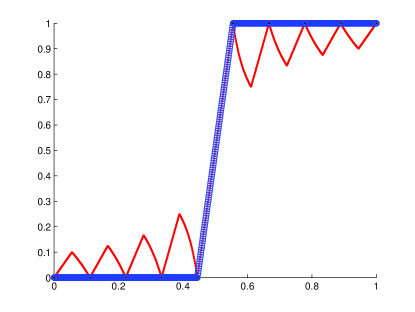
Figure 1: Comparing PMSE to AMLE on the step function.

Alternative notions of average smoothness.

One might consider a natural alternative definition of average smoothness, less stringent than our ${\overbracket{\Lambda}}$ and our ${\widetilde{\Lambda}}$:

$${\overbracket{\Lambda}}^{\sf{alt}}_{f}(\mu,\Omega)=\int_{\Omega}\int_{\Omega}\frac{|f(x)-f(y)|}{\rho(x,y)}\mathrm{d}\mu(x)\mathrm{d}\mu(y).$$

We argue that ${\overbracket{\Lambda}}^{\sf{alt}}_{f}(\mu,\Omega)$ fails as an average measure of smoothness for bounding empirical covering numbers and obtaining generalization guarantees. Indeed, consider $\Omega=[0,1]$ endowed with the standard metric $\rho(x,x^{\prime})=|x-x^{\prime}|$ and uniform distribution $\mu$. Let $\mathscr{F}$ be the collection of all $f:\Omega\to\left\{0,1\right\}$ with finite support. It is well-known that $\mathscr{F}$ is not UGC under $\mu$, and has typical empirical covering numbers exponential in sample size. However, since $|f(x)-f(y)|$ vanishes $\mu^{2}$-almost-everywhere on $[0,1]^{2}$, we have that ${\overbracket{\Lambda}}^{\sf{alt}}_{f}(\mu,\Omega)=0$ for all $f\in\mathscr{F}$. As a consistency check, note that no uniform bound over all $f\in\mathscr{F}$ is possible for either ${\overbracket{\Lambda}}_{f}$ or ${\widetilde{\Lambda}}_{f}$.

Appendix G Chernoff-type bound

Theorem 29.

For $X\sim\mathrm{Binomial}(n,p)$ and $p=p(n)\geq 2\log(n)/n$, $q=q(n)\leq p(n)/\log(n)$,

$$\mathop{\mathbb{P}}(X/n\leq q) \leq \left(\frac{e\log n}{n}\right)^{2},\qquad n\geq 3.$$ (76)

Proof.

For all $0<q<p<1$ and $X\sim\mathrm{Binomial}(n,p)$, [Dubhashi and Panconesi, 1998, page 4]

$$\mathop{\mathbb{P}}(X/n\leq q) \leq \left(\left(\frac{p}{q}\right)^{q}\left(\frac{1-p}{1-q}\right)^{1-q}\right)^{n}.$$

We first consider the case where $p(n)=2\log(n)/n$ and $q(n)=p(n)/\log(n)=2/n$. In this case,

$$\mathop{\mathbb{P}}(X/n\leq q)\cdot\left(\frac{n}{\log n}\right)^{2} \leq \left(\left(\frac{p}{q}\right)^{q}\left(\frac{1-p}{1-q}\right)^{1-q}\right)^{n}\cdot\left(\frac{n}{\log n}\right)^{2}$$

$$= (\log n)^{2}\cdot\left(\frac{n-2\log n}{n-2}\right)^{n-2}\cdot\left(\frac{n}{\log n}\right)^{2}$$

$$= n^{2}\left(\frac{n-2\log n}{n-2}\right)^{n-2}=:a(n)$$

$$\mathop{\longrightarrow}\limits_{n\to\infty} e^{2}.$$

Furthermore, the sequence $a(n)$ is monotonically increasing for $n\geq 12$, and it is easily verified that $a(n)\leq e^{2}$ for all $n\geq 3$. This proves (76) for $p(n)=2\log(n)/n$, $q(n)=2/n$.

To prove the full claim, consider the function

$$f(p,k)=k^{p/k}\left(\frac{1-p}{1-p/k}\right)^{1-p/k},\qquad p\in[0,1],k\in[1,\infty).$$

We claim that (i) $f$ is monotonically decreasing in each argument and (ii) this suffices to establish (76) in its full generality. To see how monotonicity implies the full claim, note that $\mathop{\mathbb{P}}(X/n\leq p/k)\leq f(p,k)^{n}$, the latter being maximized by the smallest feasible values of $p$ and $k$. The conditions of the Theorem constrain these at $p\geq 2\log(n)/n$ and $k\geq\log n\geq\log 3>1$, which reduces the problem to the case analyzed above.

To prove monotonicity in $p$, compute

$$\frac{\partial}{\partial p}\log f(p,k)=\frac{1-k+(1-p)\log k-(1-p)\log[(1-p)/(1-p/k)]}{k(1-p)}.$$

Since the denominator is clearly positive, it suffices to prove that the numerator is negative. Now $1-k+(1-p)\log k\leq 1-k+\log k<0$ for $k>1$, and $(1-p)/(1-p/k)>1$, so the contribution of the remaining term is negative as well.

To prove monotonicity in $k$, compute

$$\frac{\partial}{\partial k}\log f(p,k)=\frac{p[-\log k+\log((1-p)/(1-p/k))]}{k^{2}},$$

whose negativity is equivalent to $k>(1-p)/(1-p/k)$, the latter a consequence of $k>1$.

∎

References

- Ambrosio and Ghezzi (2016) L. Ambrosio and R. Ghezzi. Sobolev and bounded variation functions on metric measure spaces. In Geometry, analysis and dynamics on sub-Riemannian manifolds. Vol. II, EMS Ser. Lect. Math., pages 211–273. Eur. Math. Soc., Zürich, 2016.
- Anthony and Bartlett (1999) M. Anthony and P. L. Bartlett. Neural Network Learning: Theoretical Foundations. Cambridge University Press, Cambridge, 1999. ISBN 0-521-57353-X. doi: 10.1017/CBO9780511624216. URL http://dx.doi.org/10.1017/CBO9780511624216.
- Appell et al. (2014) J. Appell, J. Banaś, and N. Merentes. Bounded variation and around, volume 17 of De Gruyter Series in Nonlinear Analysis and Applications. De Gruyter, Berlin, 2014. ISBN 978-3-11-026507-1; 978-3-11-026511-8.
- Bartlett (2006) P. Bartlett. Covering numbers and metric entropy (lecture 23). Class Notes on Statistical Learning Theory, https://people.eecs.berkeley.edu/~bartlett/courses/281b-sp06/lecture23.ps, 2006.
- Bartlett et al. (1997) P. L. Bartlett, S. R. Kulkarni, and S. E. Posner. Covering numbers for real-valued function classes. IEEE Trans. Information Theory, 43(5):1721–1724, 1997. doi: 10.1109/18.623181. URL https://doi.org/10.1109/18.623181.
- Basu and Owen (2016) K. Basu and A. B. Owen. Transformations and Hardy-Krause variation. SIAM J. Numer. Anal., 54(3):1946–1966, 2016. ISSN 0036-1429. doi: 10.1137/15M1052184. URL https://doi.org/10.1137/15M1052184.
- Benedek and Itai (1991) G. M. Benedek and A. Itai. Learnability with respect to fixed distributions. Theoretical Computer Science, 86(2):377 – 389, 1991. ISSN 0304-3975. doi: 10.1016/0304-3975(91)90026-X. URL http://www.sciencedirect.com/science/article/pii/030439759190026X.
- Berend and Kontorovich (2013) D. Berend and A. Kontorovich. A sharp estimate of the binomial mean absolute deviation with applications. Statistics & Probability Letters, 83(4):1254–1259, 2013.
- Chaudhuri and Dasgupta (2014) K. Chaudhuri and S. Dasgupta. Rates of convergence for nearest neighbor classification. In NIPS, 2014.
- Chlamtáč (2020) E. Chlamtáč. Private Communication, 2020.
- Chlamtáč et al. (2016) E. Chlamtáč, M. Dinitz, C. Konrad, G. Kortsarz, and G. Rabanca. The densest k-subhypergraph problem. In Approximation, Randomization, and Combinatorial Optimization. Algorithms and Techniques (APPROX/RANDOM 2016), 2016.
- Cohen et al. (2020) D. Cohen, A. Kontorovich, and G. Wolfer. Learning discrete distributions with infinite support. In Neural Information Processing Systems (NIPS), 2020.
- Cohen et al. (2019) M. B. Cohen, Y. T. Lee, and Z. Song. Solving linear programs in the current matrix multiplication time. In Proceedings of the 51st annual ACM SIGACT symposium on theory of computing, pages 938–942, 2019.
- Cole and Gottlieb (2006) R. Cole and L.-A. Gottlieb. Searching dynamic point sets in spaces with bounded doubling dimension. In STOC, pages 574–583, 2006.
- Csirik et al. (1991) J. Csirik, J. Frenk, M. Labbe, and S. Zhang. Heuristics for the 0-1 min-knapsack problem. Acta Cybernetica, 10(1-2):15–20, 1991.
- Donoho and Johnstone (1998) D. L. Donoho and I. M. Johnstone. Minimax estimation via wavelet shrinkage. Ann. Statist., 26(3):879–921, 1998. ISSN 0090-5364. doi: 10.1214/aos/1024691081. URL https://doi.org/10.1214/aos/1024691081.
- Dubhashi and Panconesi (1998) D. Dubhashi and A. Panconesi. Concentration of measure for the analysis of randomised algorithms, book draft. 1998.
- Dubhashi and Panconesi (2009) D. P. Dubhashi and A. Panconesi. Concentration of Measure for the Analysis of Randomized Algorithms. Cambridge University Press, 2009. ISBN 978-0-521-88427-3. URL http://www.cambridge.org/gb/knowledge/isbn/item2327542/.
- Dudley (1999) R. M. Dudley. Uniform Central Limit Theorems. Cambridge Studies in Advanced Mathematics. Cambridge University Press, 1999. ISBN 9780521461023.
- Dutta and Nguyen (2018) P. Dutta and K. T. Nguyen. Covering numbers for bounded variation functions. J. Math. Anal. Appl., 468(2):1131–1143, 2018. ISSN 0022-247X. doi: 10.1016/j.jmaa.2018.08.062. URL https://doi.org/10.1016/j.jmaa.2018.08.062.
- Efremenko et al. (2020) K. Efremenko, A. Kontorovich, and M. Noivirt. Fast and bayes-consistent nearest neighbors. In International Conference on Artificial Intelligence and Statistics, AISTATS, 2020.
- Giné and Zinn (1984) E. Giné and J. Zinn. Some limit theorems for empirical processes. Ann. Probab., 12(4):929–998, 1984. ISSN 0091-1798. With discussion.
- Gottlieb et al. (2014) L. Gottlieb, A. Kontorovich, and R. Krauthgamer. Efficient classification for metric data (extended abstract: COLT 2010). IEEE Transactions on Information Theory, 60(9):5750–5759, 2014. doi: 10.1109/TIT.2014.2339840. URL http://dx.doi.org/10.1109/TIT.2014.2339840.
- Gottlieb et al. (2018) L. Gottlieb, A. Kontorovich, and P. Nisnevitch. Near-optimal sample compression for nearest neighbors (extended abstract: NIPS 2014). IEEE Trans. Information Theory, 64(6):4120–4128, 2018. doi: 10.1109/TIT.2018.2822267. URL https://doi.org/10.1109/TIT.2018.2822267.
- Gottlieb et al. (2016) L.-A. Gottlieb, A. Kontorovich, and R. Krauthgamer. Adaptive metric dimensionality reduction (extended abstract: ALT 2013). Theoretical Computer Science, pages 105–118, 2016.
- Gottlieb et al. (2017) L.-A. Gottlieb, A. Kontorovich, and R. Krauthgamer. Efficient regression in metric spaces via approximate Lipschitz extension (extended abstract: SIMBAD 2013). IEEE Transactions on Information Theory, 63(8):4838–4849, 2017.
- Hanneke (2018) S. Hanneke. Homework #3: ORF 525: Statististical learning and nonparametric estimation, Spring, 2018.
- Hanneke et al. (2020+) S. Hanneke, A. Kontorovich, S. Sabato, and R. Weiss. Universal bayes consistency in metric spaces. Ann. Statist., 2020+.
- Har-Peled and Mendel (2006) S. Har-Peled and M. Mendel. Fast construction of nets in low-dimensional metrics and their applications. SIAM Journal on Computing, 35(5):1148–1184, 2006. doi: 10.1137/S0097539704446281. URL http://link.aip.org/link/?SMJ/35/1148/1.
- Heinonen (2001) J. Heinonen. Lectures on analysis on metric spaces. Universitext. Springer-Verlag, New York, 2001. ISBN 0-387-95104-0. doi: 10.1007/978-1-4613-0131-8. URL http://dx.doi.org/10.1007/978-1-4613-0131-8.
- Juutinen (2002) P. Juutinen. Absolutely minimizing Lipschitz extensions on a metric space. Ann. Acad. Sci. Fenn. Math., 27(1):57–67, 2002. ISSN 1239-629X.
- Kolmogorov and Tihomirov (1961) A. N. Kolmogorov and V. M. Tihomirov. -entropy and -capacity of sets in functional space. Amer. Math. Soc. Transl. (2), 17:277–364, 1961.
- Koufogiannakis and Young (2014) C. Koufogiannakis and N. E. Young. A nearly linear-time ptas for explicit fractional packing and covering linear programs. Algorithmica, 70(4):648–674, 2014.
- Kpotufe (2011) S. Kpotufe. k-NN regression adapts to local intrinsic dimension. In Advances in Neural Information Processing Systems 24, pages 729–737, 2011. URL http://books.nips.cc/papers/files/nips24/NIPS2011_0498.pdf.
- Kpotufe and Dasgupta (2012) S. Kpotufe and S. Dasgupta. A tree-based regressor that adapts to intrinsic dimension. J. Comput. Syst. Sci., 78(5):1496–1515, Sept. 2012. ISSN 0022-0000. doi: 10.1016/j.jcss.2012.01.002. URL http://dx.doi.org/10.1016/j.jcss.2012.01.002.
- Kpotufe and Garg (2013) S. Kpotufe and V. K. Garg. Adaptivity to local smoothness and dimension in kernel regression. In Advances in Neural Information Processing Systems 26: 27th Annual Conference on Neural Information Processing Systems 2013. Proceedings of a meeting held December 5-8, 2013, Lake Tahoe, Nevada, United States., pages 3075–3083, 2013. URL http://papers.nips.cc/paper/5103-adaptivity-to-local-smoothness-and-dimension-in-kernel-regression.
- Krauthgamer and Lee (2004) R. Krauthgamer and J. R. Lee. Navigating nets: Simple algorithms for proximity search. In 15th Annual ACM-SIAM Symposium on Discrete Algorithms, pages 791–801, Jan. 2004.
- Kuipers and Niederreiter (1974) L. Kuipers and H. Niederreiter. Uniform distribution of sequences. Wiley-Interscience [John Wiley & Sons], New York-London-Sydney, 1974. Pure and Applied Mathematics.
- Ledoux and Talagrand (1991) M. Ledoux and M. Talagrand. Probability in Banach Spaces. Springer-Verlag, 1991.
- Long (2004) P. M. Long. Efficient algorithms for learning functions with bounded variation. Inf. Comput., 188(1):99–115, 2004. doi: 10.1016/S0890-5401(03)00164-0. URL https://doi.org/10.1016/S0890-5401(03)00164-0.
- Malykhin (2010) Y. V. Malykhin. Averaged modulus of continuity and bracket compactness. Mat. Zametki, 87(3):468–471, 2010. ISSN 0025-567X. doi: 10.1134/S0001434610030181. URL https://doi.org/10.1134/S0001434610030181.
- Mammen and Tsybakov (1999) E. Mammen and A. B. Tsybakov. Smooth discrimination analysis. Ann. Statist., 27(6):1808–1829, 12 1999. doi: 10.1214/aos/1017939240. URL https://doi.org/10.1214/aos/1017939240.
- Manurangsi (2017) P. Manurangsi. Almost-polynomial ratio ETH-hardness of approximating densest k-subgraph. In Proceedings of the 49th Annual ACM SIGACT Symposium on Theory of Computing, pages 954–961, 2017.
- McShane (1934) E. J. McShane. Extension of range of functions. Bull. Amer. Math. Soc., 40(12):837–842, 1934. ISSN 0002-9904. doi: 10.1090/S0002-9904-1934-05978-0. URL http://dx.doi.org/10.1090/S0002-9904-1934-05978-0.
- Mendelson and Vershynin (2003) S. Mendelson and R. Vershynin. Entropy and the combinatorial dimension. Invent. Math., 152(1):37–55, 2003. ISSN 0020-9910. doi: 10.1007/s00222-002-0266-3. URL http://dx.doi.org/10.1007/s00222-002-0266-3.
- Mohri et al. (2012) M. Mohri, A. Rostamizadeh, and A. Talwalkar. Foundations Of Machine Learning. The MIT Press, 2012.
- Nickl and Pötscher (2007) R. Nickl and B. M. Pötscher. Bracketing metric entropy rates and empirical central limit theorems for function classes of Besov- and Sobolev-type. J. Theoret. Probab., 20(2):177–199, 2007. ISSN 0894-9840. doi: 10.1007/s10959-007-0058-1. URL https://doi.org/10.1007/s10959-007-0058-1.
- Niederreiter and Talay (2006) H. Niederreiter and D. Talay, editors. Monte Carlo and quasi-Monte Carlo methods 2004, 2006. Springer-Verlag, Berlin. ISBN 978-3-540-25541-3; 3-540-25541-9. doi: 10.1007/3-540-31186-6. URL https://doi.org/10.1007/3-540-31186-6.
- Oberman (2008) A. M. Oberman. An explicit solution of the Lipschitz extension problem. Proc. Amer. Math. Soc., 136(12):4329–4338, 2008. ISSN 0002-9939. doi: 10.1090/S0002-9939-08-09457-4. URL https://doi.org/10.1090/S0002-9939-08-09457-4.
- Peres et al. (2009) Y. Peres, O. Schramm, S. Sheffield, and D. B. Wilson. Tug-of-war and the infinity Laplacian. J. Amer. Math. Soc., 22(1):167–210, 2009. ISSN 0894-0347. doi: 10.1090/S0894-0347-08-00606-1. URL https://doi.org/10.1090/S0894-0347-08-00606-1.
- Sendov and Popov (1988) B. Sendov and V. A. Popov. The averaged moduli of smoothness. Pure and Applied Mathematics (New York). John Wiley & Sons, Ltd., Chichester, 1988. ISBN 0-471-91952-7. Applications in numerical methods and approximation, A Wiley-Interscience Publication.
- Shawe-Taylor et al. (1998) J. Shawe-Taylor, P. L. Bartlett, R. C. Williamson, and M. Anthony. Structural risk minimization over data-dependent hierarchies. IEEE Transactions on Information Theory, 44(5):1926–1940, 1998.
- Shvartsman (2017) P. Shvartsman. Whitney-type extension theorems for jets generated by Sobolev functions. Adv. Math., 313:379–469, 2017. ISSN 0001-8708. doi: 10.1016/j.aim.2017.04.009. URL https://doi.org/10.1016/j.aim.2017.04.009.
- Tsybakov (2004) A. B. Tsybakov. Introduction à l’estimation non-paramétrique, volume 41 of Mathématiques & Applications (Berlin) [Mathematics & Applications]. Springer-Verlag, Berlin, 2004. ISBN 3-540-40592-5.
- Urner and Ben-David (2013) R. Urner and S. Ben-David. Probabilistic Lipschitzness: A niceness assumption for deterministic labels. In Learning Faster from Easy Data - NIPS Workshop, 2013.
- Vershynin (2018) R. Vershynin. High-dimensional probability, volume 47 of Cambridge Series in Statistical and Probabilistic Mathematics. Cambridge University Press, Cambridge, 2018. ISBN 978-1-108-41519-4. doi: 10.1017/9781108231596. URL https://doi.org/10.1017/9781108231596. An introduction with applications in data science, With a foreword by Sara van de Geer.
- Wainwright (2019) M. J. Wainwright. High-Dimensional Statistics: A Non-Asymptotic Viewpoint (Cambridge Series in Statistical and Probabilistic Mathematics). Cambridge University Press, 2019. ISBN 1108498027. URL https://www.amazon.com/High-Dimensional-Statistics-Non-Asymptotic-Statistical-Probabilistic/dp/1108498027?SubscriptionId=AKIAIOBINVZYXZQZ2U3A&tag=chimbori05-20&linkCode=xm2&camp=2025&creative=165953&creativeASIN=1108498027.
- Whitney (1934) H. Whitney. Analytic extensions of differentiable functions defined in closed sets. Transactions of the American Mathematical Society, 36(1):63–89, 1934. ISSN 00029947. URL http://www.jstor.org/stable/1989708.