Transformer with Depth-Wise LSTM

Abstract

Increasing the depth of models allows neural models to model complicated functions but may also lead to optimization issues. The Transformer translation model employs the residual connection to ensure its convergence. In this paper, we suggest that the residual connection has its drawbacks, and propose to train Transformers with the depth-wise LSTM which regards outputs of layers as steps in time series instead of residual connections, under the motivation that the vanishing gradient problem suffered by deep networks is the same as recurrent networks applied to long sequences, while LSTM Hochreiter and Schmidhuber (1997) has been proven of good capability in capturing long-distance relationship, and its design may alleviate some drawbacks of residual connections while ensuring the convergence. We integrate the computation of multi-head attention networks and feed-forward networks with the depth-wise LSTM for the Transformer, which shows how to utilize the depth-wise LSTM like the residual connection. Our experiment with the 6-layer Transformer shows that our approach can bring about significant BLEU improvements in both WMT 14 English-German and English-French tasks, and our deep Transformer experiment demonstrates the effectiveness of the depth-wise LSTM on the convergence of deep Transformers. Additionally, we propose to measure the impacts of the layer’s non-linearity on the performance by distilling the analyzing layer of the trained model into a linear transformation and observing the performance degradation with the replacement. Our analysis results support the more efficient use of per-layer non-linearity with depth-wise LSTM than with residual connections.

1 Introduction

The multi-layer structure allows neural models to model complicated functions. Increasing the depth of models can increase their capacity but may also cause optimization difficulties Mhaskar et al. (2017); Telgarsky (2016); Eldan and Shamir (2016); He et al. (2016); Bapna et al. (2018).

Specifically with the Transformer translation model, in order to ease its optimization, Vaswani et al. (2017) employ residual connection He et al. (2016) and layer normalization Ba et al. (2016) techniques which have been proven useful in reducing optimization difficulties of deep neural networks for various tasks.

When it comes to deep Transformers, previous works Bapna et al. (2018); Wang et al. (2019); Zhang et al. (2019); Xu et al. (2020b) are under the motivation to ensure that outputs of initial layers can be conveyed with significance to the final prediction stage, so those layers can receive sufficient gradients of good quality (mostly aiming to train their outputs for the prediction of ground-truth), i.e. they attempt to prevent residual connections from shrinking Zhang et al. (2019); Xu et al. (2020b) or to compensate probably faded residual connections Bapna et al. (2018); Wang et al. (2019); Wei et al. (2020).

In this paper, we first shed light on the problems of residual connection which can simply and effectively ensure the convergence of deep neural networks. Additionally, we propose to train Transformers with the depth-wise LSTM which regards outputs of layers as steps in time series instead of residual connections, under the motivation that deep models have difficulty in convergence because shallow layers cannot receive clear gradients from the loss function which is far away from them (their outputs cannot clearly convey to the classifier in the forward propagation), while LSTM Hochreiter and Schmidhuber (1997) has been proven of good capability in capturing long-distance relationship even though it performs better with short sentences Linzen et al. (2016), and it may alleviate some drawbacks of residual connections (we will discuss later) while ensuring the convergence.

Though to generalize the advantages of LSTM to deep computation is already proposed by Kalchbrenner et al. (2016), suggesting that the vanishing gradient problem suffered by deep networks is the same as recurrent networks applied to long sequences. We suggest that in our work, we explicitly propose to alternate residual connections with the depth-wise LSTM of the advanced, strong and popular Transformer, which is non-trival. Besides, our approach to integrate the computation of multi-head attention networks and feed-forward networks with the depth-wise LSTM for the Transformer is also more complex than their work which solely connects LSTM cells across the stacking of LSTM layers, we show how to utilize the depth-wise LSTM like the residual connection.

Our contributions in this paper are as follows:

• We suggest that the popular residual connection has its drawbacks, and propose to use depth-wise LSTM for the training of Transformers instead of using residual connections, which is non-trival.

• We integrate the depth-wise LSTM with the other parts (multi-head attention networks and feed-forward networks) of Transformer layers, which demonstrates how to use depth-wise LSTM to replace residual connections.

• In our experiments, we show that the 6-layer Transformer using depth-wise LSTM can bring significant improvements over that with residual connections. In deep Transformer experiments, we show that depth-wise LSTM also has the ability to ensure deep Transformers with up to $24$ layers, and the 12-layer Transformer using depth-wise LSTM already performs comparably to the 24-layer Transformer with residual connections, which suggests more efficient using of per-layer parameters with depth-wise LSTM than residual connections.

• To measure the effects of the non-linearity of the layer on performance, we propose to distill the analyzing layer of the trained model into a linear transformation which cannot sustain any non-linearity and observe the performance degradation brought by the replacement.

2 Preliminaries: Residual Connection and its Issue

He et al. (2016) present the residual learning framework to ease the training of deep neural networks, by explicitly reformulating the layers as learning residual functions with reference to the layer inputs, instead of learning unreferenced functions.

Specifically, they suggest that if the added layers of the deep model on top of these shallow layers are identity mapping, the deep model shall produce no higher training error than its shallower counterpart, and attribute the convergence issue of deep networks stacking non-linear layers to that it is hard for non-linear layers to learn the identity function which means that their training will encounter more difficulties than the layer which can easily model the identity function. Thus, they propose to explicitly enable these layers fit a residual mapping:

$$F(x)=H(x)+x$$ (1)

where x is the input to the non-linear layer, H(x) and F(x) are the function of that non-linear layer and that of the corresponding residual layer.

As it is easier for almost all non-linear layers to learn a zero function which consistently outputs zeros than to learn the identity function, He et al. (2016) suggest that residual connections can reduce the training difficulty of deep neural networks, and with the help of the residual connection, they successfully train the deep convolutional network up to $152$ layers with high performances on various tasks.

The Transformer Vaswani et al. (2017) also employs the residual connection to ensure the convergence of the 6-layer model, and further empirical results show that as long as the residual connection is not normalized by the layer normalization, Transformers with more than $6$ layers can also converge Wang et al. (2019); Xu et al. (2020b) with further improvements.

However, we suggest that the motivation under the residual connection, which tries to ensure each layer can learn the identity function, seems in contrast to the motivation of using deep models, to model complicated functions with the non-linearity. As a result, the residual connection, which adds the input to the output of the layer aiming to allow the model skipping one or more layers, may waste the non-linearity provided by those skipped layers, i.e. the complexity of the model function. Correspondingly in practice, it is a common observation that the improvements in performances are also smaller and smaller with the increasing of depth, and deep models seem to have difficulty in using parameters as efficient as their shallow counterparts.

In this paper, we suggest that the residual connection which simply accumulates representations of various layers with the element-wise addition operation may have the following drawbacks:

• It accumulates outputs of layers equally and lacks an evaluation mechanism to combine representations based on their importance and reliability. As a result, it may lead to two problems: 1) residual models may require many layers to overcome outputs of poor quality from few layers. 2) For deep models which aggegates outputs of many layers into a fixed dimension vector, it is likely to incur information loss, which means that a part of the layer may work on generating representations which are never used.

• After the addition of two representations, there is no way for subsequent layers to distinguish involved representations, which may bring challenge to the layer when it requires to utilize different-level of information (e.g. linguistic properties of different levels for NLP) differently.

3 Transformer with Depth-Wise LSTM

3.1 Depth-Wise LSTM and its Advantages

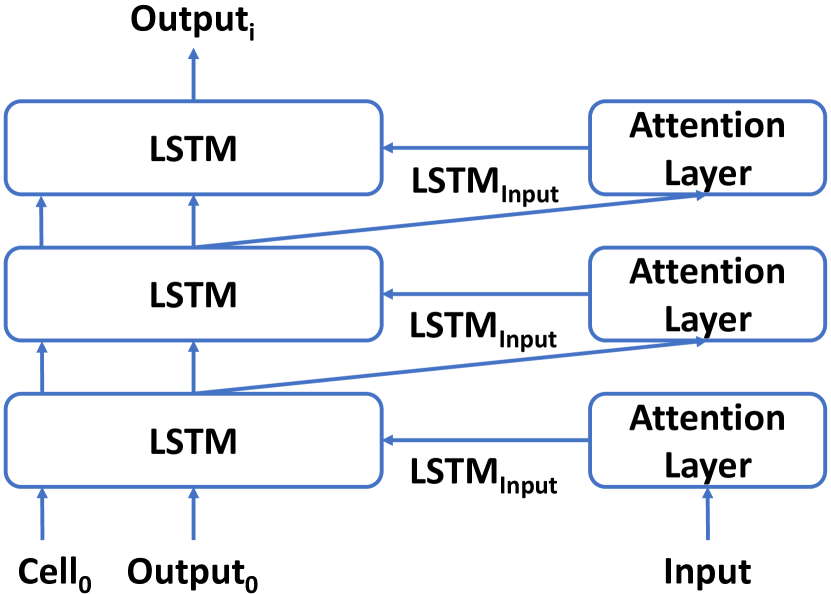
Figure 1: Transformer with Depth-Wise LSTM

Intuitively, deep models have difficulty in convergence because shallow layers cannot receive clear gradients from the loss which is far away from them (their outputs cannot clearly convey to the classifier in the forward propagation). The LSTM which is able to capture long-distance relationship (use the representation of a far token for the computing of current token), shall be able to utilize the output of the first layer in the computing of the last layer while using it in a depth-wise way (regarding layer depth as a token sequence). Thus, we suggest to alternate the residual connection with the depth-wise LSTM which forward propagates steps with outputs of layers in a layer-by-layer manner instead of the token-by-token manner, as illustrated in Figure 1.

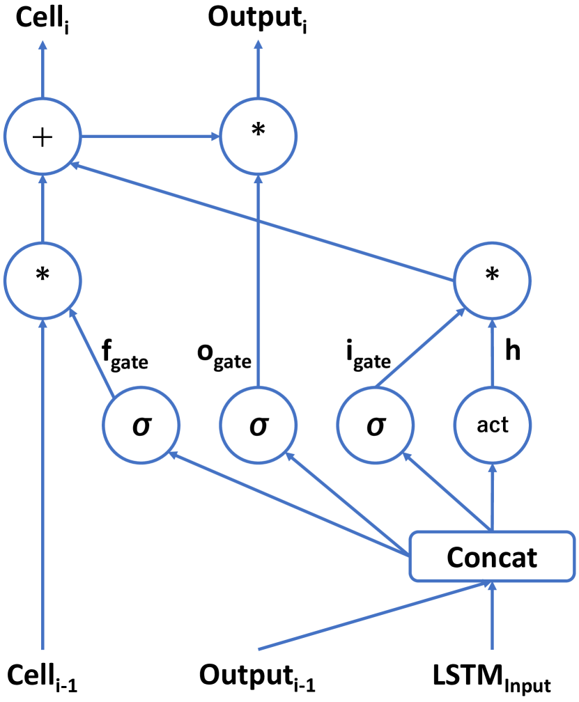
Figure 2: LSTM Computation. Layer Normalization is omitted for simplicity.

We employ the LSTM equipped with layer normalization in this work following Chen et al. (2018), which provides better performance as the NMT decoder than the vanilla LSTM. The computation graph of the LSTM is shown in Figure 2.

Specifically, it first concatenates the input $LSTM_{Input}$ to the LSTM with the output of the LSTM in the last step $Output_{i-1}$:

$${\rm{c}}=LSTM_{Input}|Output_{i-1}$$ (2)

where “$|$” indicates concatenation and “$c$” is the concatenated vector.

Then, the LSTM computes three gates (specifically, input gate $i_{gate}$, forget gate $f_{gate}$ and output gate $o_{gate}$) together with the hidden representation $h$ with the concatenated representation:

$${{\rm{i}}_{{\rm{gate}}}}=\sigma(LN({W_{ig}}c+{b_{ig}}))$$ (3)

$${{\rm{f}}_{{\rm{gate}}}}=\sigma(LN({W_{fg}}c+{b_{fg}}))$$ (4)

$${{\rm{o}}_{{\rm{gate}}}}=\sigma(LN({W_{og}}c+{b_{og}}))$$ (5)

$$h=act(LN({W_{h}}c+{b_{h}}))$$ (6)

where $W_{*}$ and $b_{*}$ are weight and bias parameters, $\sigma$ is the sigmoid activation function, “LN” is the layer normalization, “$act$” stands for the activation function for the computation of the hidden state.

The layer normalization Ba et al. (2016) is computed as follows:

$$LN_{Output}=\frac{{LN_{Input}-\mu}}{{{\sigma}}}*w_{LN}+b_{LN}$$ (7)

where $LN_{Input}$ and $LN_{Output}$ are the input and corresponding computation result of the layer normalization, $\mu$ and $\sigma$ stand for the mean and standard deviation of $LN_{Input}$, $w_{LN}$ and $b_{LN}$ are two vector parameters initialized by ones and zeros respectively.

In this work, we use the advanced GeLU activation function Hendrycks and Gimpel (2016) which are employed by BERT Devlin et al. (2019) rather than the tanh function used in Hochreiter and Schmidhuber (1997); Chen et al. (2018).

We suppose that the role of the computation of the hidden state in Equation 6 is similar to the position-wise feed-forward sub-layer in each encoder layer and decoder layer, so we remove the feed-forward sub-layer from encoder and decoder layers while additionally study the effects of computing the hidden state with the 2-layer feed-forward network like adopted in Transformer layers, in which case, the feed-forward sub-layer is integrated as part of the computation of the depth-wise LSTM, as shown in Equation 8.

$$h=W_{h2}act(LN({W_{h1}}c+{b_{h1}}))+b_{h2}$$ (8)

After the computation of the hidden state, the cell and the output of the LSTM unit are computed as:

$$Cell_{i}=Cell_{i-1}\bullet{f_{gate}}+h\bullet{i_{gate}}$$ (9)

$$Output_{i}=Cell_{i}\bullet{o_{gate}}$$ (10)

where $\bullet$ indicates the element-wise multiplication.

Compared to the residual connection, we suggest that: 1) The gate mechanism (in Equation 3, 4, 5) of the depth-wise LSTM can serve as the evaluation mechanism to treat representations from different sources differently. 2) the computation of its hidden state (in Equation 6) is performed on the concatenated representation instead of the element-wise added representation, which allows to utilize different-level of information differently.

We use depth-wise LSTM rather than depth-wise multi-head attention network with which can build the NMT model solely based on the attention mechanism for two reasons:

• Even using the multi-head attention network, it has to compute in the layer-by-layer manner like in the decoding, which will not help GPU parallelization and bring significant acceleration.

• The attention mechanism linearly combines representations with attention weights. Thus, it lacks the ability to provide the non-linearity compared to the LSTM, which we suggest shall be important.

3.2 Encoder Layer with Depth-Wise LSTM

Directly replacing residual connections with LSTM units will introduce huge amount of additional parameters and computation. Given that the task to compute of the LSTM hidden state is similar to the feed-forward sub-layer in the original Transformer layers, we propose to replace the feed-forward sub-layer with the newly introduced LSTM unit, which only introduces one LSTM unit per layer.

The original Transformer encoder layer only contains two sub-layers: the self-attention sub-layer based on the multi-head attention network to collect information from contexts, and the 2-layer feed-forward network sub-layer to evolve representations with its non-linearity.

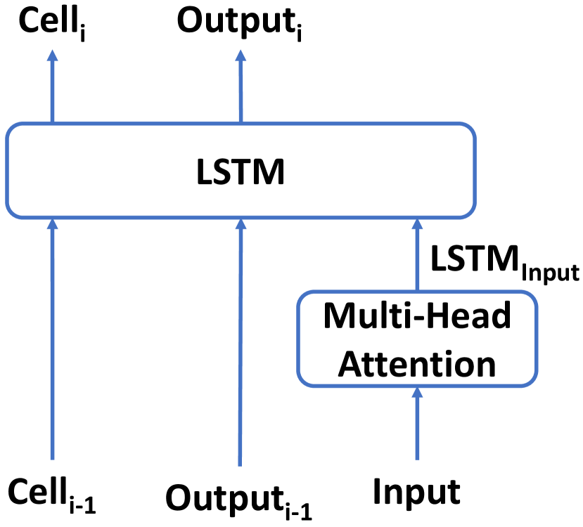
Figure 3: Encoder Layer with Depth-Wise LSTM

For the new encoder layer with the depth-wise LSTM unit (forward propagating across the depth dimension rather than the token dimension) instead of the residual connection, the layer first performs the self-attention computation, then the depth-wise LSTM unit takes the self-attention results and the output and the cell of previous layer to compute the output and the cell of current layer. The architecture of the encoder layer with depth-wise LSTM unit is shown in Figure 3.

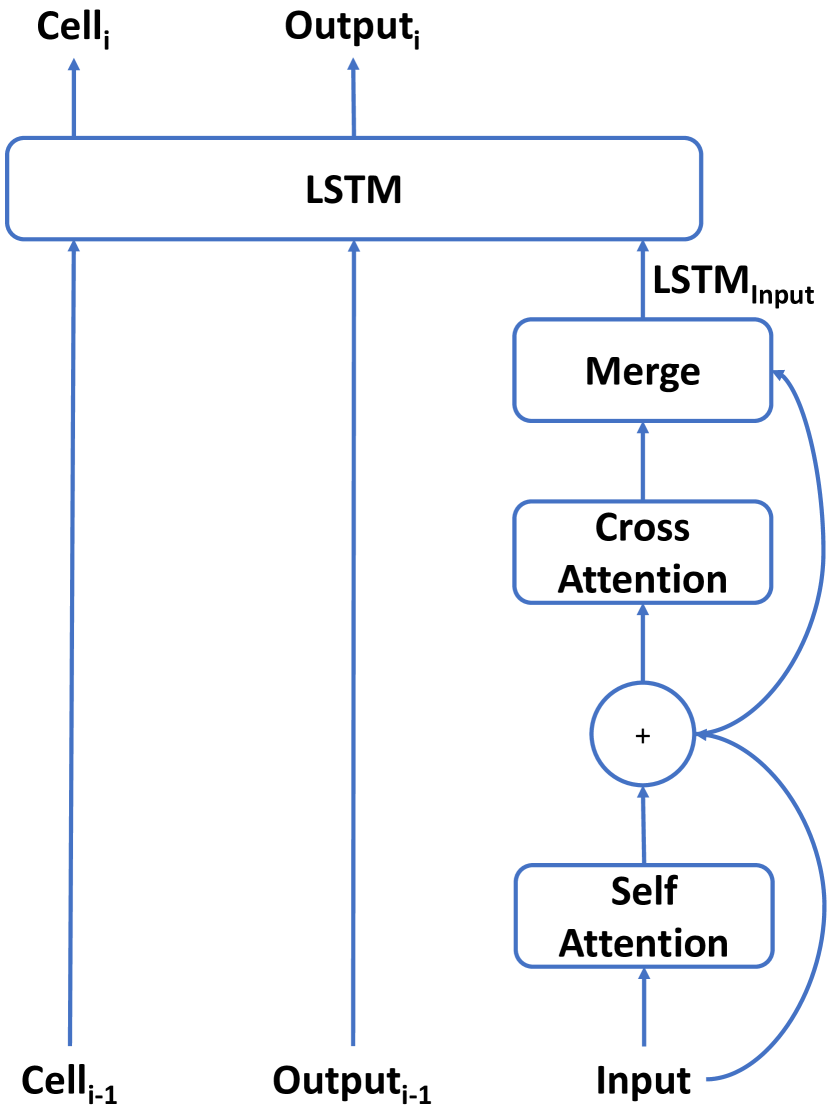
Figure 4: Decoder Layer with Depth-Wise LSTM

3.3 Decoder Layer with Depth-Wise LSTM

Different from the encoder layer, the decoder layer involves two multi-head attention sub-layers, the self-attention sub-layer to attend decoding history and the cross-attention sub-layer to bring information from the source side. Given that the depth-wise LSTM unit only takes one input, we introduce a merge layer to collect the outputs of these two sub-layers and merge them into one as the input to the LSTM unit.

Specifically, the decoder layer with depth-wise LSTM first computes the self-attention sub-layer and the cross-attention sub-layer like in the original decoder layer, then it merges the outputs of these two sub-layers and feeds the merged representation into the depth-wise LSTM unit which also takes the cell and the output of previous layer to compute the output of current decoder layer and the cell of the LSTM. We examine both element-wise addition and concatenation as the merging operation. The architecture is shown in Figure 4.

For the input of the cross-attention sub-layer, we also utilize the sum of the self-attention outputs and the input to this decoder layer like in the standard decoder layer, to utilize both self-attention results and the outputs of previous layer. Since the computation of the LSTM hidden (Equation 6 or 8) does not add its input to its output, which breaks residual connections across layers, we suggest that it is not a residual connection.

4 Analysis of Layer’s Non-Linearity on Performance

As suggested above, the residual connection eases the optimization of deep models by explicitly enabling it modeling the identity function, which may hamper the non-linearity of layers and lead to less complex model functions in contrast to the motivation of modeling a complicated function by stacking layers. How does the non-linearity provided by the layer affect the performance?

We propose to measure the contribution of a layer’s non-linearity to performance through replacing the analyzing layer of the fully trained model with a linear transformation which cannot sustain any non-linearity and observing the performance degradation brought by the replacement.

Specifically, in the standard forward propagation of the converged model, the function $F$ of the layer computes the output $y$ of that layer given its input $x$:

$$y=F(x)$$ (11)

To analyze the impacts of the non-linearity of that layer on the performance, we change its computation to:

$$y=W_{d}x+b_{d}$$ (12)

where $W_{d}$ and $b_{d}$ are the weight matrix the bias trained on the same training set with the other parts of the well trained model frozen.

The training of $W_{d}$ aims to distill the linear transformation in the function $F$ to $W_{d}$ while removing all non-linear transformation in $F$, since Equation 12 does not have any capability in providing non-linearity.

We suggest that the performance reduction resulted by removing the non-linearity of the layer through changing its computation from the original design (Equation 11) to the linear transformation (Equation 12) reveals the effects of the layer’s linearity on performance.

5 Experiment

We implemented our approach based on the Neutron implementation of the Transformer Xu and Liu (2019). To show the effects of our approach on the 6-layer Transformer, we first conducted our experiments on the WMT 14 English to German and English to French news translation tasks to compare with Vaswani et al. (2017). Additionally, we also examined the impacts of our approach on deep Transformers, experiments were conducted on the WMT 14 English to German task and the WMT 15 Czech to English task following Bapna et al. (2018); Xu et al. (2020b).

The concatenation of newstest 2012 and newstest 2013 was used for validation and newstest 2014 as test sets for the WMT 14 English to German and English to French news translation tasks, and newstest 2013 as validation set for the WMT 15 Czech to English task. Newstest 2014 was test sets for both the WMT 14 English to German and the English to French task, and newstest 2015 was the test set for the Czech to English task.

5.1 Settings

We applied joint Byte-Pair Encoding (BPE) Sennrich et al. (2016) with $32k$ merging operations on both data sets to address the unknown word issue. We only kept sentences with a maximum of $256$ subword tokens for training. Training sets were randomly shuffled in every training epoch.

Though Zhang et al. (2019); Xu et al. (2020a) suggest using a large batch size which may lead to improved performance, we used a batch size of $25k$ target tokens which was achieved through gradient accumulation of small batches to fairly compare with previous work Vaswani et al. (2017); Xu et al. (2020b). The training steps for Transformer Base and Transformer Big were $100k$ and $300k$ respectively following Vaswani et al. (2017).

The number of warm-up steps was set to $8k$, and each training batch contained at least $25k$ target tokens. We used a dropout of $0.1$ for all experiments except for the Transformer Big on the En-De task which was $0.3$. For the Transformer Base setting, the embedding dimension and the hidden dimension of the position-wise feed-forward neural network were $512$ and $2,048$ respectively, corresponding values for the Transformer Big setting were $1024$ and $4096$ respectively. We employed a label smoothing Szegedy et al. (2016) value of $0.1$. We used the Adam optimizer Kingma and Ba (2015) with $0.9$, $0.98$ and $10^{-9}$ as $\beta_{1}$, $\beta_{2}$ and $\epsilon$. We followed Vaswani et al. (2017) for the other settings.

For deep Transformers, we used the computation order of: layer normalization $\rightarrow$ processing $\rightarrow$ dropout $\rightarrow$ residual connection, which is able to converge without introducing additional approaches which may affect the performance according to Wang et al. (2019); Xu et al. (2020b).

We used a beam size of $4$ for decoding, and evaluated tokenized case-sensitive BLEU with the averaged model of the last $5$ checkpoints for the Transformer Base setting and $20$ checkpoints for the Transformer Big setting saved with an interval of $1,500$ training steps. We also conducted significance tests Koehn (2004).

5.2 Main Results

We first examine the effects of our approach on the 6-layer Transformer on the WMT 14 English-German and English-French task to compare with Vaswani et al. (2017), and results are shown in Table 1.

Models	En-De	En-Fr
Transformer Base	27.55	39.54
with depth-wise LSTM	28.41†	40.02†
Transformer Big	28.63	41.52
with depth-wise LSTM	29.42†	43.04†

Table 1: Results on WMT 14 En-De and En-Fr. ^† indicates $p<0.01$ in significance test.

In our approach (“with depth-wise LSTM”), we used the 2-layer neural network for the computation of the LSTM hidden state (as in Equation 8) and shared parameters across stacked encoder / decoder layers for computing the LSTM gates (in Equation 3, 4, 5). Further details can be found in our ablation study.

Table 1 shows that our approach to use the depth-wise LSTM for the convergence of the Transformer can bring significant improvements on both tasks over the Transformer with residual connections with both the Transformer Base setting and the Transformer Big Setting.

We conjecture that our approach with the base setting brings about more improvements on the English-German task than that on the English-French task may because that the performance on the English-French task using a large dataset ($\sim 36M$) may rely more on the capability of the model (i.e. the number of parameters) than on the complexity of the modeling function (i.e. depth of the model, non-linearity strength per-layer, etc.). With the Transformer Big model which contains more parameters than the Transformer Base, the improvement on En-Fr ($+1.52$) is larger than that on En-De ($+0.79$).

5.3 Ablation Study

We first study the effects of two types of computations for the LSTM hidden in Equation 6 and 8 on performance on the WMT 14 En-De task. Results are shown in Table 2.

FFN	BLEU
LSTM	27.84
2-Layer	28.41

Table 2: Ablation Study of LSTM Hidden Computation.

Table 2 shows that the 2-layer feed-forward neural network used in Transformer layers outperforms the original computation of the LSTM hidden which uses only one layer, which is consistent with intuition.

We also study two merging operations, the concatenation and element-wise addition, to combine the self-attention sub-layer output and the cross-attention sub-layer output for the depth-wise LSTM unit in decoder layers. Results are shown in Table 3.

Merging	BLEU
Concat	28.28
Add	28.41

Table 3: Results of Merging Operations for Decoder Layer

Table 3 shows that though counter intuitively, the element-wise addition merging operation empirically results in slightly higher BLEU than the concatenation operation with fewer parameters introduced. Thus, we use the element-wise addition operation in our experiments by default.

Since the number of layers is pre-specified, the depth-wise LSTM unit in all layers can either be shared or be independent (i.e. whether to bind parameters of the depth-wise LSTM across stacked layers). Since Table 2 supports the importance of the capability of the module for the hidden state computation, and sharing the module is likely to hurt its capability, we additionally study to share only parameters for gate computation (in Equation 3, 4, 5) and to share all parameters (i.e. parameters for both the computation of gates and that of the hidden state). Results are shown in Table 4.

Sharing	BLEU
All	26.89
Gate	28.41
None	28.21

Table 4: Results of Sharing LSTM Parameters.

Table 4 shows that: 1) Sharing parameters for the computation of the LSTM hidden significantly hampers its performance, which is consistent with our conjecture. 2) Sharing parameters for the computation of gates (in Equation 3, 4, 5) leads to slightly higher BLEU with fewer parameters introduced than without sharing them (“None” in Table 4). Thus, in the other experiments, we bind parameters for the computation of LSTM gates across stacked layers by default.

5.4 Deep Transformers

To examine whether the depth-wise LSTM has the ability to ensure the convergence of deep Transformers and how it performs with deep Transformers. We conduct experiments on the WMT 14 English to German task and the WMT 15 Czech to English task following Bapna et al. (2018); Xu et al. (2020b), and compare our approach with the Transformer in which residual connections are not normalized by layer normalization. Results are shown in Table 5.

Layers	En-De		Cs-En
	Std	Ours	Std	Ours
6	27.55	28.41	28.40	29.05
12	28.12	29.20	29.38	29.60
18	28.60	29.23	29.61	30.08
24	29.02	29.09	29.73	29.95

Table 5: Results of Deep Transformers. Std and Ours mean the standard Transformer with residual connection and our approach with depth-wise LSTM respectively.

Table 5 shows that though the BLEU improvements seem saturated with deep Transformers more than $12$ layers, depth-wise LSTM is able to ensure the convergence of the up to $24$ layer Transformer.

On the En-De task, the 12-layer Transformer with depth-wise LSTM already outperforms the 24-layer Transformer with residual connections, suggesting the efficient using of layer parameters.

On the Cs-En task, the 12-layer model with our approach performs comparably to the 24-layer model with residual connections. Unlike the En-De task, increasing depth over the 12-layer Transformer can still bring some BLEU improvements, and the 18-layer model results in the best performance. We conjecture that probably because the data set of the Cs-En task ($\sim 10M$) is larger than that of the En-De task ($\sim 4.5M$), and increasing the depth of the model for the Cs-En task also increasing its number of parameters and capability. While for the En-De task, the 12-layer Transformer with depth-wise LSTM may already provide both sufficient complexity and capability for the data set.

5.5 Layer Non-Linearity Analysis

Layer	Encoder		Decoder
	BLEU	$\Delta\ (\%)$	BLEU	$\Delta\ (\%)$
None	27.55	0.00	27.55	0.00
1	27.17	-1.38	27.62	0.25
2	27.11	-1.60	27.64	0.33
3	27.09	-1.67	27.47	-0.29
4	27.07	-1.74	27.53	-0.07
5	27.15	-1.45	26.96	-2.14
6	27.24	-1.13	26.42	-4.10

Table 6: Per-Layer Performance Reduction of the 6-Layer Transformer Base.

Layer	Encoder		Decoder
	BLEU	$\Delta\ (\%)$	BLEU	$\Delta\ (\%)$
None	28.41	0.00	28.41	0.00
1	27.50	-3.20	28.30	-0.39
2	26.60	-6.37	28.17	-0.84
3	27.09	-4.65	28.22	-0.67
4	27.41	-3.52	28.05	-1.27
5	27.87	-1.90	26.82	-5.60
6	27.84	-2.01	19.87	-30.06

Table 7: Per-Layer Performance Reduction of the 6-Layer Transformer Base with Depth-Wise LSTM.

To study the contribution of each layer to the over all performance (i.e. how the output of each layer is utilized by the other layers and the classifier in the translation), we perform the layer efficiency analysis on the WMT 14 En-De task. We use the performance reduction in BLEU to show the contribution of individual layers to the overall performance. Non-linearity removing results of the 6-layer standard Transformer with residual connections and the corresponding model with the depth-wise LSTM are shown in Table 6 and 7 respectively. BLEU and $\Delta$ indicate the BLEU score after distilling the layer into the linear transformation and its relative reduction compared to the full model performance (in percentages).

Compared to Table 6, Table 7 shows that the normalized performance loss of each layer with the depth-wise LSTM is larger than that with residual connections, with which we suggest that individual layers trained with the depth-wise LSTM get a more important role in the overall performance than those trained with residual connections.

Another interesting observation is that, though the performance degradation of removing the non-linearity of decoder layer 1 to 3 of the Transformer with depth-wise LSTM are relatively small, suggesting the possible redundancy of the 6-layer decoder, surprisingly, removing the non-linearity of the first and second decoder layer of the 6-layer standard Transformer with residual connections even leads to slight BLEU improvements, which supports our first suggestion of the drawbacks brought by residual connections (described in Section 2) and the first advantage of using depth-wise LSTM (described in Section 3.1). We conjecture that residual connections may try to train the first and second decoder layer to linear transformations. However, its goal is not fully achieved until the end of the training, while the evaluation mechanism (gates) of the depth-wise LSTM helps ensure the non-linearity of the layer at least does not degrade the performance.

6 Related Work

He et al. (2016) suggest that the non-linear activation function makes the layer without the residual connection has difficulty in learning the identity function, thus the model without residual connections suffer from severer convergence problem than the model with residual connections, and present the residual learning framework to ease the training of deep neural networks, by explicitly reformulating the layers as learning residual functions with reference to the layer inputs, instead of learning unreferenced functions. Srivastava et al. (2015) propose the highway network which contains a transform gate and a carry gate to control how much of the output is produced by transforming the input and carrying it, respectively. More recently, Chai et al. (2020) propose the highway Transformer, which integrates a self-gating mechanism into the Transformer. However, we suggest our work is quite different from it, e.g. residual connections are still kept in their model.

Deep NMT.

Zhou et al. (2016) introduce the fast-forward connections and an interleaved bi-directional architecture for stacking the LSTM layers which play an essential role in propagating the gradients and building a deep topology of depth $16$. Wang et al. (2017) propose a novel Linear Associative Unit (LAU) which uses linear associative connections between input and output of the recurrent unit to reduce the gradient propagation path inside.

Deep Transformers.

Bapna et al. (2018) propose the Transparent Attention (TA) mechanism which improves gradient flow during back propagation by allowing each decoder layer to attend weighted combinations of all encoder layer outputs, instead of just the top encoder layer. Wang et al. (2019) propose the Dynamic Linear Combination of Layers (DLCL) approach which additionally aggregate previous layers’ outputs for each encoder layer. Wu et al. (2019) propose an effective two-stage approach which incrementally increases the depth of the encoder and the decoder of the Transformer Big model by freezing both parameters and the encoder-decoder attention computation of pre-trained shallow layers. More recently, Wei et al. (2020) let each decoder layer attend the corresponding encoder layer of the same depth and introduce a depth-wise GRU to additionally aggregate outputs of all encoder layers for the top decoder layer, but residual connections are still kept in their approach. Zhang et al. (2019) propose the layer-wise Depth-Scaled Initialization (DS-Init) approach, which decreases parameter variance at the initialization stage, and reduces output variance of residual connections so as to ease gradient back-propagation through normalization layers. Xu et al. (2020b) propose the Lipschitz constrained parameter initialization approach to reduce the standard deviation of layer normalization inputs and to ensure the convergence of deep Transformers.

7 Conclusion

In this paper, we suggest that the popular residual connection has its drawbacks. Inspired by that the vanishing gradient problem suffered by deep networks is the same as recurrent networks applied to long sequences Kalchbrenner et al. (2016), we alternate residual connections of the Transformer with the depth-wise LSTM ,which propogates through the depth dimension rather than the sequence dimension, given that LSTM Hochreiter and Schmidhuber (1997) has been proven of good capability in capturing long-distance relationship, and its design may alleviate some drawbacks of residual connections while ensuring the convergence. Specifically, we show how to integrate the computation of multi-head attention networks and feed-forward networks with the depth-wise LSTM for the Transformer, and how to utilize the depth-wise LSTM like the residual connection.

Our experiment with the 6-layer Transformer shows that our approach using depth-wise LSTM can bring about significant BLEU improvements in both WMT 14 English-German and English-French tasks over the standard Transformer with residual connections. Our deep Transformer experiment demonstrates that: 1) Our depth-wise LSTM approach also has the ability to ensure deep Transformers with up to $24$ layers, 2) The 12-layer Transformer using depth-wise LSTM already performs comparably to the 24-layer Transformer with residual connections, suggesting more efficient usage of per-layer parameters with our depth-wise LSTM approach than with residual connections.

We propose to measure how the non-linearity of the layer affects performance by replacing the analyzing layer of the trained model with a linear transformation which cannot sustain any non-linearity and observing the performance degradation brought by the replacement. Our analysis results support the more efficient use of per-layer non-linearity of the Transformer with depth-wise LSTM than that with residual connections.

References

- Ba et al. (2016) Jimmy Lei Ba, Jamie Ryan Kiros, and Geoffrey E Hinton. 2016. Layer normalization. arXiv preprint arXiv:1607.06450.
- Bapna et al. (2018) Ankur Bapna, Mia Chen, Orhan Firat, Yuan Cao, and Yonghui Wu. 2018. Training deeper neural machine translation models with transparent attention. In Proceedings of the 2018 Conference on Empirical Methods in Natural Language Processing, pages 3028–3033. Association for Computational Linguistics.
- Chai et al. (2020) Yekun Chai, Shuo Jin, and Xinwen Hou. 2020. Highway transformer: Self-gating enhanced self-attentive networks. In Proceedings of the 58th Annual Meeting of the Association for Computational Linguistics, pages 6887–6900, Online. Association for Computational Linguistics.
- Chen et al. (2018) Mia Xu Chen, Orhan Firat, Ankur Bapna, Melvin Johnson, Wolfgang Macherey, George Foster, Llion Jones, Mike Schuster, Noam Shazeer, Niki Parmar, Ashish Vaswani, Jakob Uszkoreit, Lukasz Kaiser, Zhifeng Chen, Yonghui Wu, and Macduff Hughes. 2018. The best of both worlds: Combining recent advances in neural machine translation. In Proceedings of the 56th Annual Meeting of the Association for Computational Linguistics (Volume 1: Long Papers), pages 76–86, Melbourne, Australia. Association for Computational Linguistics.
- Devlin et al. (2019) Jacob Devlin, Ming-Wei Chang, Kenton Lee, and Kristina Toutanova. 2019. BERT: Pre-training of deep bidirectional transformers for language understanding. In Proceedings of the 2019 Conference of the North American Chapter of the Association for Computational Linguistics: Human Language Technologies, Volume 1 (Long and Short Papers), pages 4171–4186, Minneapolis, Minnesota. Association for Computational Linguistics.
- Eldan and Shamir (2016) Ronen Eldan and Ohad Shamir. 2016. The power of depth for feedforward neural networks. In 29th Annual Conference on Learning Theory, volume 49 of Proceedings of Machine Learning Research, pages 907–940, Columbia University, New York, New York, USA. PMLR.
- He et al. (2016) K. He, X. Zhang, S. Ren, and J. Sun. 2016. Deep residual learning for image recognition. In 2016 IEEE Conference on Computer Vision and Pattern Recognition (CVPR), pages 770–778.
- Hendrycks and Gimpel (2016) Dan Hendrycks and Kevin Gimpel. 2016. Gaussian error linear units (gelus). CoRR, abs/1606.08415.
- Hochreiter and Schmidhuber (1997) Sepp Hochreiter and Jürgen Schmidhuber. 1997. Long short-term memory. Neural Comput., 9(8):1735–1780.
- Kalchbrenner et al. (2016) Nal Kalchbrenner, Ivo Danihelka, and Alex Graves. 2016. Grid long short-term memory. In 4th International Conference on Learning Representations, ICLR 2016, San Juan, Puerto Rico, May 2-4, 2016, Conference Track Proceedings.
- Kingma and Ba (2015) Diederik P. Kingma and Jimmy Ba. 2015. Adam: A method for stochastic optimization. In 3rd International Conference on Learning Representations, ICLR 2015, San Diego, CA, USA, May 7-9, 2015, Conference Track Proceedings.
- Koehn (2004) Philipp Koehn. 2004. Statistical significance tests for machine translation evaluation. In Proceedings of the 2004 Conference on Empirical Methods in Natural Language Processing.
- Linzen et al. (2016) Tal Linzen, Emmanuel Dupoux, and Yoav Goldberg. 2016. Assessing the ability of LSTMs to learn syntax-sensitive dependencies. Transactions of the Association for Computational Linguistics, 4:521–535.
- Mhaskar et al. (2017) Hrushikesh Mhaskar, Qianli Liao, and Tomaso Poggio. 2017. When and why are deep networks better than shallow ones? In Proceedings of the Thirty-First AAAI Conference on Artificial Intelligence, pages 2343–2348.
- Sennrich et al. (2016) Rico Sennrich, Barry Haddow, and Alexandra Birch. 2016. Neural machine translation of rare words with subword units. In Proceedings of the 54th Annual Meeting of the Association for Computational Linguistics (Volume 1: Long Papers), pages 1715–1725. Association for Computational Linguistics.
- Srivastava et al. (2015) Rupesh Kumar Srivastava, Klaus Greff, and Jürgen Schmidhuber. 2015. Highway networks. CoRR, abs/1505.00387.
- Szegedy et al. (2016) C. Szegedy, V. Vanhoucke, S. Ioffe, J. Shlens, and Z. Wojna. 2016. Rethinking the inception architecture for computer vision. In 2016 IEEE Conference on Computer Vision and Pattern Recognition (CVPR), pages 2818–2826.
- Telgarsky (2016) Matus Telgarsky. 2016. benefits of depth in neural networks. In 29th Annual Conference on Learning Theory, volume 49 of Proceedings of Machine Learning Research, pages 1517–1539, Columbia University, New York, New York, USA. PMLR.
- Vaswani et al. (2017) Ashish Vaswani, Noam Shazeer, Niki Parmar, Jakob Uszkoreit, Llion Jones, Aidan N Gomez, Ł ukasz Kaiser, and Illia Polosukhin. 2017. Attention is all you need. In Advances in Neural Information Processing Systems 30, pages 5998–6008. Curran Associates, Inc.
- Wang et al. (2017) Mingxuan Wang, Zhengdong Lu, Jie Zhou, and Qun Liu. 2017. Deep neural machine translation with linear associative unit. In Proceedings of the 55th Annual Meeting of the Association for Computational Linguistics (Volume 1: Long Papers), pages 136–145, Vancouver, Canada. Association for Computational Linguistics.
- Wang et al. (2019) Qiang Wang, Bei Li, Tong Xiao, Jingbo Zhu, Changliang Li, Derek F. Wong, and Lidia S. Chao. 2019. Learning deep transformer models for machine translation. In Proceedings of the 57th Conference of the Association for Computational Linguistics, pages 1810–1822, Florence, Italy. Association for Computational Linguistics.
- Wei et al. (2020) Xiangpeng Wei, Heng Yu, Yue Hu, Yue Zhang, Rongxiang Weng, and Weihua Luo. 2020. Multiscale collaborative deep models for neural machine translation. In Proceedings of the 58th Annual Meeting of the Association for Computational Linguistics, pages 414–426, Online. Association for Computational Linguistics.
- Wu et al. (2019) Lijun Wu, Yiren Wang, Yingce Xia, Fei Tian, Fei Gao, Tao Qin, Jianhuang Lai, and Tie-Yan Liu. 2019. Depth growing for neural machine translation. In Proceedings of the 57th Annual Meeting of the Association for Computational Linguistics, pages 5558–5563, Florence, Italy. Association for Computational Linguistics.
- Xu et al. (2020a) Hongfei Xu, Josef van Genabith, Deyi Xiong, and Qiuhui Liu. 2020a. Dynamically adjusting transformer batch size by monitoring gradient direction change. In Proceedings of the 58th Annual Meeting of the Association for Computational Linguistics, pages 3519–3524, Online. Association for Computational Linguistics.
- Xu and Liu (2019) Hongfei Xu and Qiuhui Liu. 2019. Neutron: An Implementation of the Transformer Translation Model and its Variants. arXiv preprint arXiv:1903.07402.
- Xu et al. (2020b) Hongfei Xu, Qiuhui Liu, Josef van Genabith, Deyi Xiong, and Jingyi Zhang. 2020b. Lipschitz constrained parameter initialization for deep transformers. In Proceedings of the 58th Annual Meeting of the Association for Computational Linguistics, pages 397–402, Online. Association for Computational Linguistics.
- Zhang et al. (2019) Biao Zhang, Ivan Titov, and Rico Sennrich. 2019. Improving deep transformer with depth-scaled initialization and merged attention. In Proceedings of the 2019 Conference on Empirical Methods in Natural Language Processing and the 9th International Joint Conference on Natural Language Processing (EMNLP-IJCNLP), pages 898–909, Hong Kong, China. Association for Computational Linguistics.
- Zhou et al. (2016) Jie Zhou, Ying Cao, Xuguang Wang, Peng Li, and Wei Xu. 2016. Deep recurrent models with fast-forward connections for neural machine translation. Transactions of the Association for Computational Linguistics, 4:371–383.