Tackling solvent effect by coupling electronic and molecular Density Functional Theory

Abstract

Solvation effect might have a tremendous influence on chemical reactions. However, precise quantum chemistry calculations are most often done either in vacuum neglecting the role of the solvent or using continuum solvent model ignoring its molecular nature. We propose a new method coupling a quantum description of the solute using electronic density functional theory with a classical grand-canonical treatment of the solvent using molecular density functional theory. Unlike previous work, both densities are minimised self consistently, accounting for mutual polarisation of the molecular solvent and the solute. The electrostatic interaction is accounted using the full electron density of the solute rather than fitted point charges. The introduced methodology represents a good compromise between the two main strategies to tackle solvation effect in quantum calculation. It is computationally more effective than a direct quantum-mechanics/molecular mechanics coupling, requiring the exploration of many solvent configurations. Compared to continuum methods it retains the full molecular-level description of the solvent. We validate this new framework onto two usual benchmark systems: a water solvated in water and the symmetrical nucleophilic substitution between chloromethane and chloride in water. The prediction for the free energy profiles are not yet fully quantitative compared to experimental data but the most important features are qualitatively recovered. The method provides a detailed molecular picture of the evolution of the solvent structure along the reaction pathway.

I Introduction

The solvent is often described as the media in which a chemical reaction between dissolved species, called solutes, takes place. However, it is well known that besides its role of bringing the reactants in contact, the solvent has a tremendous influence on the chemical reaction as it impacts the kinetics and the thermodynamics of the reaction. Organic chemists have taken advantage of these solvent effects since decades. For instance, in the 30’s, Hughes and Ingold already discussed a theory of solvation effect for nucleophilic substitution ($\text{S}_{\text{N}}$) (Hughes and Ingold, 1935). In this paper, they reviewed the already substantial experimental work on the influence of the choice of solvent on the $\text{S}_{\text{N}}$ reaction and they proposed a theoretical model accounting for solvent effect. Hughes and Ingold model is based on a simple hypothesis: only electrostatic interactions are considered. By examining the stabilising and/or destabilising role of the solvent on the reactants, products and transition states of the reaction they were able to rationalise effect of solvent polarity on reaction rates. However, solvent molecules may also be directly involved in the reaction mechanism. For instance, Liu et al have shown that adding a single methanol molecule largely promotes the $\text{S}_{\text{N}}$ reaction with respect to elimination reaction (Liu et al., 2018). Direct involvement of solvent molecules cannot be captured by macroscopic consideration as the ones used in Hughes and Ingold model. A good alternative is to resort to molecular simulation. Since chemical reaction involves formation and/or breaking of chemical bonds it makes the use of classical force field difficult: even if reactive force field exist, their parametrisation are often costly and difficult (Han et al., 2016; Senftle et al., 2016). Thus, to study chemical reaction the first approach is often to use a Quantum Mechanics (QM) based method such as electronic density functional theory (eDFT), Hartree Fock or more advanced technique such as Moller-Plesset or Coupled Cluster. Due to computational cost, such calculations are often run in vacuum and at 0 K which neglect solvent effect.

To incorporate solvent effect, the most natural choice is to explicitly include solvent molecules into the simulation. This is extremely costly since it increases considerably the number of electrons with respect to in-vacuo calculations. The finite temperature is even more problematic since the meaningful quantity is no longer the ground state energy but the free energy. This means that the calculation should take place in a statistical ensemble and that a long enough trajectory should be produced to compute ensemble average with good statistics (Frenkel and Smit, 2002). This is the typical setup of ab-initio Molecular Dynamics (AIMD) calculations (Silvestrelli and Parrinello, 1999). The problem of free energy calculation is particularly difficult since it cannot be written as a (grand) canonical average over the phase space (Frenkel and Smit, 2002). For those two reasons AIMD simulations are limited to efficient QM techniques. There are almost always based on eDFT and only small systems can be investigated.

To circumvent the computational cost of AIMD a natural choice is to split the studied system into 2 parts. A first one, which is considered as essential for the description of the chemistry is treated at the QM level. A second one, which often includes most of the solvent molecules, for which interactions are described by molecular mechanics (MM) using classical force fields. This is the well known QM/MM approach which has been used successfully to tackle a wide variety of systems (Lin and Truhlar, 2007). The MM part is most often dealt with Molecular Dynamics (MD) or Monte Carlo (MC). While QM/MM makes it possible to considerably reduce the numerical cost of evaluating forces as compared to AIMD, the problem of computing free energy remains. A further simplification is to average out the solvent degrees of freedom to reduce tremendously the dimensionality of the problem and the computational cost. This is the strategy adopted in continuum solvent models (CSM) approaches such as the polarisable continuum model (PCM) (Tomasi and Persico, 1994; Tomasi et al., 2005; Klamt, 2011) where the solvent is described by a dielectric continuum. CSM have been applied with success but it suffers from several drawbacks. First, it contains several ah-hoc parameters that are not physically based but are rather optimised on reference calculations. Second, it completely loses the description of the solvent at the molecular level.

Another way to tackle solvation problem is to conserve the QM/MM partition of the system but to use liquid state theories to deal with the MM part. Liquid state theories have proven efficient to describe simple liquids such as hard-sphere or Lennard-Jones fluids (Hansen and McDonald, 2006). Several approaches such as integral equation theory, its interaction site approximation (RISM) (Chandler and Andersen, 1972) or classical density functional theory (cDFT) (Ebner et al., 1976) have been applied in that context. The common objective of all these techniques is to find the equilibrium number solvent density $n$($\bm{r}$), or equivalently its total correlation function $h(\bm{r})$. For simple liquid such as hard-sphere or Lennard-Jones fluid these fields solely depends on the position of the solvent $\bm{r}$. A key quantity entering all these theories is the direct correlation function between solvent molecules $c(r)$.

More recent development have made possible to tackle realistic molecular fluids such as water or acetonitrile, either based on the integral equation theory (Belloni and Chikina, 2014) or the molecular density functional theory (MDFT) (Ramirez et al., 2002; Zhao et al., 2011; Jeanmairet et al., 2013a, b, 2015, 2016, 2019a, 2019b). In a molecular solute-solvent system the density field $\rho(\bm{r},\bm{\Omega})$ no longer depends solely on the position $\bm{r}$ but also on the orientation $\bm{\Omega}$ of the solvent. Consequently the direct correlation function $c(\bm{r},\bm{\Omega}_{1},\bm{\Omega}_{2})$ becomes extremely complicated as it now depends on a position vector and two orientations.

The RISM approach and its 3D-RISM (Kovalenko and Hirata, 1998) generalisation circumvent this problem by averaging out the solvent orientation. The complicated molecular correlation function $c$ is replaced by simpler 1D site-site correlation functions. The gain in efficiency is obvious but it is at the price of working with site-site OZ equation and site-site correlation functions which are no longer based on a proper statistical physics derivation. Another approach based on molecular density functional theory (MDFT) has ben proposed recently to solve the MOZ equation, with the hypernetted chain (HNC) closure, without making such approximations. The use of projections onto rotational invariants allows to handle the numerically costly angular convolution products (Ding et al., 2017) making the method practical.

Liquid state theories represent a good compromise between CSM and MD based approaches since it conserves the description of solvent as made of molecular entities while not requiring the tedious statistical sampling of solvent degrees of freedom. It is thus natural to propose a formalism where solutes are described using QM and solvent using liquid state theories. Since the original paper (Ten-no et al., 1993), numerous studies using RISM (Naka et al., 1999) or 3D-RISM (Sato et al., 2000; Kasahara and Sato, 2018; Kaminski et al., 2010; Zhou et al., 2011) have been done to study solvation effect on a solute described by QM. This method is implemented in widely distributed quantum codes such as ADF (Gusarov et al., 2006; Casanova et al., 2007). Because the development of classical DFT techniques to study molecular liquids are more recent, less attempt have been done to describe solvation of QM solutes with this method. The Arias group have developed the joint DFT framework (Petrosyan et al., 2005, 2007) and released the code JDFTx (Sundararaman et al., 2017) where the method is implemented. The classical DFT fluids that are implemented in JDFTx are using functional based on model molecular Hamiltonian that are parametrised to reproduce some feature of the liquid such as its non-local dielectric response on external electric field —an improvement over PCM. However the performance of this simplified DFT approach to reproduce molecular properties is not completely satisfying (Sundararaman et al., 2012; Sundararaman and Arias, 2014).

Zhao et al recently proposed the so-called Reaction Density Functional Theory (RxDFT) (Tang et al., 2018; Cai et al., 2019; Tang et al., 2020) which is based on MDFT. In this approach the solute energy is computed using eDFT. Then the solute is described classically by a set of Lennard-Jones sites and point charges in a subsequent MDFT calculation to estimate the solvation free energy. The classical charges are fitted to reproduce the molecular electrostatic potential (ESP) computed in the QM calculation. This is a first limitation since there is no unique way to determine the ESP charges as illustrated by the variety of existing fitting methods (Sigfridsson and Ryde, 1998; Marenich et al., 2012; Hu et al., 2007). Another limitation is the absence of polarisation of the QM solute under the influence of non homogeneous solvent density in RxDFT. The ESP charges are fitted using electronic densities computed in vacuum or using a CSM. This method thus actually consists in a MDFT calculation with a force field where the charges have been reparametrised on a prior eDFT calculation rather than in a self-consistent QM/MDFT procedure.

The purpose of this paper is to address these limitations and to propose a QM/MDFT procedure where the quantum part and the MDFT part are optimised self-consistently. Moreover, in contrast to the common practise in QM/MM approaches, the solute electronic density is directly used in the MDFT calculation which prevent to use ill-defined atomic point charges. The rest of the paper is organised as follow, first we present the theoretical aspects of the coupling between QM and MDFT before testing the proposed methodology on two commonly-used benchmarks. We first focus on the solvation of an eDFT water molecule in MDFT water before addressing an aqueous chemical reaction namely a symmetric nucleophilic substitution between chloromethane and chloride.

II Theory

The solvation free energy (SFE) $\Delta F$ can be defined as the difference between the free energy of the solute-solvent system and the sum of the free energies of the solute in vacuum and of the pure solvent as depicted in figure 1.a. It is a key quantity to understand chemistry in solution. For instance, SFE difference between the products and the reactants, figure 1.b, is directly linked to the equilibrium constant of the reaction. Similarly, the difference between the SFE of the same solute in two different solvents allow to compute partition constant. The aim of this paper is to propose a joint self-consistent eDFT/MDFT approach to evaluate the SFE.

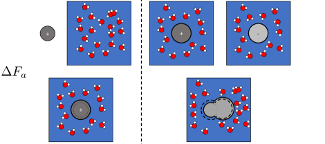
Figure 1: Thermodynamic scheme for the computation of solvation free energy (left) and reaction free energy (right). The electronic density of the solute is schematised by a solid black line. Dashed line represent the electronic density in the previous state.

We first start by our standard formulation of molecular density functional theory. In MDFT, the solvent molecules are assumed to be rigid entities interacting through a classical force field. Since molecules are rigid, the knowledge of the position of their centre of mass (COM) $\bm{r}$ and their orientation $\bm{\Omega}$ are sufficient to fully described molecule coordinates. In this paper we only consider SPC/E water as a solvent but we proposed functional for other molecular fluids such as acetonitrile in the past (Borgis et al., 2012). The DFT ansatz states that for any external perturbation it is possible to write a unique functional $F$ of the solvent density $\rho$ (Evans, 1979). At its minimum, which is reached for the equilibrium density $\rho_{\text{eq}}$, the functional $F$ equals the SFE $\Delta F$. MDFT is thus particularly appropriate to compute SFE since it requires a functional minimisation while brute force MD would require a costly sampling. The functional $F$ is usually written as

$$F[\rho]=F_{\text{id}}[\rho]+F_{\text{ext}}[\rho]+F_{\text{exc}}[\rho].$$ (1)

The solvent density $\rho(\bm{r},\bm{\Omega})$ is a 6D field that depends on the space coordinate and the orientation $\bm{\Omega}$.

In equation 1 the ideal term $F_{\text{id}}$ corresponds to the entropic term of the non-interacting fluid (Hansen and McDonald, 2006). The third term $F_{\text{exc}}$ is due to solvent-solvent interaction (Jeanmairet et al., 2013b). In this work we use the expression proposed by Ding et al for SPC/E (Ding et al., 2017), which corresponds to the so-called hypernetted chain for the excess functional $F_{\text{exc}}$. The remaining term $F_{\text{ext}}$ is due to the external perturbation acting on the liquid, here the solute. This last term represents the solute-solvent interaction and can formally be written as

$$F_{\text{ext}}[\rho]=\iint\rho\left(\bm{r},\bm{\bm{\Omega}}\right)V_{\text{ext}}(\bm{r},\bm{\Omega})d\bm{r}d\bm{\Omega}.$$ (2)

where $V_{\text{ext}}$ is the external energy density.

In our previous work (Jeanmairet et al., 2013a, b, 2015, 2016, 2019b, 2019a; Levesque et al., 2012) the solute was described by a classical force field, usually a set of Lennard-Jones and point charges. Here we describe the solute quantum mechanically using eDFT. Using the DFT ansatz (Hohenberg and Kohn, 1964), it exists a functional $F_{e}$ of the electronic density $\rho_{e}$ which is equal to the ground state energy at its minimum. The electrostatic interaction between the quantum solute and the classical solvent can easily be expressed in a mean field way

$$E_{\text{ES}}[\rho,\rho_{e}]=\iint\frac{\sigma_{\text{V}}(\bm{r})\sigma_{\text{U}}(\bm{r}^{\prime})}{4\pi\epsilon_{0}\left|\bm{r}-\bm{r}^{\prime}\right|}d\bm{r}d\bm{r}^{\prime}$$ (3)

where $\sigma_{\text{V}}$ is the charge density of the solvent and $\sigma_{\text{U}}$ is the charge density of the solute. Each of these charge density is related to the corresponding particle density. The solute charge density is

$$\sigma_{\text{U}}(\bm{r})=\sum_{i}Z_{i}\delta(\bm{r}-\bm{r}_{i})-\rho_{e}(\bm{r})$$ (4)

where $Z_{i}$ is the atomic number of nucleus $i$ located in $\bm{r}_{i}$. The solvent charge density can be expressed as

$$\sigma_{\text{V}}(\bm{r})=\iint\rho(\bm{r},\bm{\Omega})\sigma(\bm{r}-\bm{r}^{\prime},\bm{\Omega})d\bm{r}^{\prime}d\bm{\Omega}.$$ (5)

where $\sigma(\bm{r},\bm{\Omega})$ is the charge density of a water molecule taken at the origin with orientation $\bm{\Omega}$.

The electrostatic contribution to the external term of equation 2 can thus be computed injecting equations 4-5 in equation 3. However, short-range repulsion and dispersion interactions are not taken into account. To do so, similarly to QM/MM calculations, we resort to Lennard-Jones sites located on nuclei of the solute. Since there is no prescriptions on how to choose the Lennard-Jones parameters the common practice is to resort to generic force fields such as OPLS (Tirado-Rives and Jorgensen, 2019) or CHARMM (Riccardi et al., 2004). However, the solvation free energy and the solvation structure depend on the LJ parameters (Tu and Laaksonen, 1999; Riccardi et al., 2004). That is why, as any QM/MM calculation, the present approach cannot be considered as being truly ab-initio. A more elegant and ab-initio way would be to use some electron-solvent pseudo-potential to account for the repulsion-dispersion interactions (Vaidehi et al., 1992). This strategy has been widely applied to study solvated electrons in liquids or clusters (Schnitker and Rossky, 1987; Turi and Borgis, 2002; Mones and Turi, 2010). Eventually, the external term of the functional can be written as

$$F_{\text{ext}}[\rho,\rho_{e}]=E_{\text{ES}}[\rho,\rho_{e}]+\iint\rho\left(\bm{r},\bm{\bm{\Omega}}\right)V_{\text{LJ}}(\bm{r},\bm{\Omega})d\bm{r}d\bm{\Omega}.$$ (6)

with

$$V_{\text{LJ}}(\bm{r},\bm{\Omega}) = \sum_{i\in\text{solute}}\sum_{j\in\text{solvent}}4\epsilon_{ij}\left[\left(\frac{\sigma_{ij}}{\left|\bm{r}+\bm{r}_{j\Omega}-\bm{r}_{i}\right|}\right)^{12}\right.$$

$$-\left.\left(\frac{\sigma_{ij}}{\left|\bm{r}+\bm{r}_{j\Omega}-\bm{r}_{i}\right|}\right)^{6}\right]$$

where $\epsilon_{ij}$ and $\sigma_{ij}$ are the mixed Lennard-Jones parameters using the Lorentz-Berthelot rules, $\bm{r}_{i}$ is the position of the $i^{\text{th}}$ site of the solute and $\bm{r}_{j\Omega}$ denotes the position with respect to the COM of site $j$ of a solvent molecule located in $\bm{r}$ with orientation $\bm{\Omega}$.

As opposed to our previous work where the solute was described classically, the free energy of the solute is modified when transferred from the gas phase to the solute. We approximate this free energy difference $\Delta F_{\text{QM}}$ by the energy difference at $T=0\ K$ which is much easier to compute. This neglects the nuclear and electronic fluctuations.

$$\Delta F_{\text{QM}}[\rho_{e}]\approx\Delta E_{\text{QM}}[\rho_{e}]=F_{e}[\rho_{e}]-F_{e}[\rho_{e}^{\text{vac}}]$$ (7)

where $\rho_{e}^{\text{vac}}$ is the equilibrium electronic density in vacuum. Finally, using equations 1,6 and 7 the solvation free energy can be computed by minimising the functional

$$F\left[\rho_{e},\rho\right]=\Delta E_{\text{QM}}[\rho_{e}]+F_{\text{id}}[\rho]+F_{\text{ext}}[\rho]+F_{\text{exc}}[\rho_{e},\rho]$$ (8)

with respect to the electronic density $\rho_{e}(\bm{r})$ and the solvent density $\rho(\bm{r},\bm{\Omega})$.

Instead of carrying the joint minimisation we adopt a simpler strategy. First, the electronic functional is minimised in vacuum. The equilibrium electronic density is then used in the MDFT calculation to compute the electrostatic contribution to external term using equation 3. After minimisation of the MDFT functional, the equilibrium solvent charge density is used to compute the electrostatic external potential acting on the electronic density using equation 3. The electronic functional is minimised and a new electronic density is obtained. This process is repeated until both the electronic energy of equation 7 and the solvation free energy of equation 1 are converged to a given threshold. Using this procedure, the electrostatic energy of equation 3 is computed twice, once in the electronic DFT calculation and once in the MDFT one. These two values can be compared as a sanity check to verify convergence.

We insist on the fact that the full electronic density of the quantum solute is used in the computation of electrostatic interaction between the QM and the MM part in equation 3. It differs from the strategy usually adopted in QM/MM calculation that consists in computing partial point charges from the electronic density (Lin and Truhlar, 2007). Since there is no unique way to determine these charges (Marenich et al., 2012; Sigfridsson and Ryde, 1998; Sifain et al., 2018) and since it is difficult to evaluate their quality a posteriori it is advantageous to circumvent this parametrisation and work directly with the electronic density.

The self-consistent optimisation of electronic density $\rho_{e}(\bm{r})$ and the solvent density $\rho(\bm{r},\bm{\Omega})$ when minimising equation 8 allows to account for the mutual polarisation of the solute and the solvent environment. This is a clear improvement with respect to methods that consists in single QM calculation in vacuum followed by a single liquid state theory calculation such as RxDFT (Tang et al., 2018; Cai et al., 2019; Tang et al., 2020). Indeed, such methods neglect the polarisation of the solute by the solvent density which is properly accounted with the present approach.

A last strength of the present approach is that it retains a proper description of the solvent at the molecular level. The equilibrium solvent density contains a detailed 3D picture of the solvent location and orientations around the solute which is not accessible to continuum models or simpler liquid state theories.

III Applications

III.1 Water in water.

As a first test of the QM/MDFT framework introduced in II, we focus on the “water in water” system. A single water molecule, referred as the solute, is immersed in water solvent described by MDFT. The solute is treated at the eDFT level with the PBE functional. Calculations are run using the GPAW package (Enkovaara et al., 2010; Larsen et al., 2017; Mortensen et al., 2005). Wave functions are expanded on a real space grid. The volume of the simulation cell is $5\times 5\times 5$ $\textrm{\r{A}}^{3}$ and details about the grid resolution are given after. The geometry of the solute is the one of the SPC/E molecule.

Solvent calculations are done using our homemade MDFT code, the water model is SPC/E. We used a cubic cell of $25\times 25\times 25\ \textrm{\r{A}}^{3}$. The orientational space $\text{SO}(3)$ is discretised with 196 orientations, the space grid resolution is specified further. Our homemade fortran written MDFT program was interfaced with Python using f90wrap which makes the coupling with GPAW easy.

Dispersion forces are modelled using Lennard-Jones sites located on the solute atoms in the MDFT calculation. The Lennard-Jones parameters of the oxygen of the solute are the same as in SPC/E. The Lennard-Jones parameters on hydrogens are $\sigma=1.0\ \textrm{\r{A}}$ and $\epsilon=0.0234$ kJ.mol^-1. This almost non attractive Lennard-Jone site prevent numerical divergence due to “unshielded” charges, this trick has already been used in RISM-SCF studies (Ten-no et al., 1993, 1994).

We first check the validity of the implementation by comparing the external electrostatic energies obtained in the QM and in the MDFT calculations according to equation 3. For this test there are $n^{3}$ points in the QM grid and $8\ n^{3}$ in the MDFT one where $n=32,40,48,64$. The convergence criterion on the relative variation is 10^-4 for both the QM energy and the MDFT free energy. Results are reported in table 1. In all cases the electrostatic energies agree within 1%. For $n=32$ the resolution of the grids are clearly not sufficient since the results differs by 5 $\text{kJ.mol}^{-1}$ from the one obtained with finer grids. If $n=32$ is omitted, the finer the grid the better is the agreement between the two ways to evaluate the electrostatic energy.

$n$	QM $\left(\text{kJ.mol}{}^{-1}\right)$	MDFT $\left(\text{kJ.mol}{}^{-1}\right)$	$\frac{\text{QM}}{\text{MDFT}}$
32	-54.5077	-54.4329	1.0014
40	-59.5362	-59.8865	0.9942
48	-59.1667	-59.3552	0.9968
64	-59.1093	-59.2150	0.9982

Table 1: Final external electrostatic energy of water in water computed according to equation 3. The second column is the result obtained with the QM code, the result obtained with MDFT is displayed in the third column. The fourth column show the ratio of the second and third column. There are $n^{3}$ nodes on the QM grid and $8n^{3}$ on the MDFT grid.

After this numerical test we run calculation on the same system with $48^{3}$ grid nodes on the QM grid and $120^{3}$ nodes on the MDFT space grid. We use a convergence criterion of 10^-4 on the relative variation of QM energy and MDFT free energy. The electronic energies and solvation free energies as a function of the iteration step are displayed in figure 2. While it requires 42 iterations to reach the required criterion only 5 iterations are necessary to reach a criterion of $10^{-3}$. As expected, solvation stabilises the solute: the QM energy at convergence is $0.58\ \text{eV}$ lower than in the initial state i.e. in vacuum. In a similar way, the solvation free energy computed by MDFT is reduced by $6.6\ \text{kJ.mo$\text{l}^{-1}$}$ when the electronic density is optimised.

Moreover, the polarisation of the solvent influences the electronic density of the solute. This effect can only be captured if the electronic density and the solvent density are optimised self-consistently.

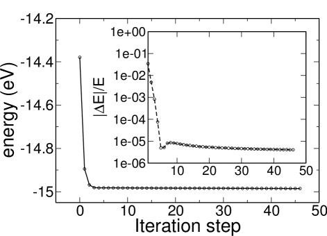
Figure 2: Energy of the quantum solute as computed by eDFT (top) and its solvation free energy as computed by MDFT (down) as a function of the iteration step. In insets are the relative differences of these quantities.

The solvation free energy of water computed using equation 8 is $-3.4\ \text{kJ.mo$\text{l}^{-1}$}$. It is clearly overestimated when compared to the experimental value of $-26.5\ \text{kJ.mol}{}^{-1}$ but also to the value of $-29.5\ \text{kJ.mol}{}^{-1}$ which is the one of the SPC/E model computed using MD. Using the continuum solvent model implemented in GPAW (Held and Walter, 2014) gives a solvation free energy of $-27.0\ \text{kJ.mol}{}^{-1}$ in better agreement with the experimental value. The overestimation of solvation free energy is a known problem of the HNC functional as already illustrated for the TIP3P model (Luukkonen et al., 2020) and is mostly due to the quadratic form of the functional, which cause a tremendous overestimation of the pressure (Jeanmairet et al., 2013a, 2015). We have proposed several physically based bridge functionals to correct this flaw and go beyond the HNC level. It is also possible to stay at the HNC level and simply use a one parameter a posteriori cavity correction of the SFE (Luukkonen et al., 2020). Using this simple correction, we obtain a solvation free energy of $-20.2\ \text{kJ.mol}{}^{-1}$, in better agreement with the experimental value but still overestimated.

Unfortunately, the imperfection of the functional is not the sole defect of our calculation. Predictions of the solvation free energy are also quite sensitive to the the choice of Lennard-Jones parameters. To illustrate this point we computed the solvation free energy of water changing only the Lennard-Jones site on the Oxygen of the solute. We have taken the values of $\sigma$ and $\epsilon$ for some popular water model: SPC/E, OPC, TIP3P and TIP4P. We emphasise that the geometry of the solute is not changed. The SFE computed using these parameters are displayed in table 2 and they vary by up to 1.5 $\text{kJ.mol}^{-1}$.

	$\sigma$ $\left(\textrm{\r{A}}\right)$	$\epsilon$ $\left(\text{kJ.mol}{}^{-1}\right)$	$\Delta F$ $\left(\text{kJ.mol}{}^{-1}\right)$
TIP3P	3.15061	0.6364	-20.3
TIP4P	3.1589	0.7749	-19.5
OPC3	3.165	0.9945	-18.8
SPC/E	3.17427	0.65	-20.2

Table 2: Solvation Free energy of water obtained using different Lennard-Jones parameters for the solute described using eDFT, its geometry is always the one of SPC/E.

After examining the energetics, we now turn to the solvation structure. The radial distribution functions (rdf) between oxygen of the solvent and atomic sites of the solute are displayed in figure 3. First, we recall that the agreement between the experimental rdf and the one computed by MD for the SPC/E model is good (Soper, 2000; Mark and Nilsson, 2001). The agreement is less satisfying for the rdf predicted by MDFT using the HNC functional as previously reported for SPC/E and TIP3P (Jeanmairet et al., 2013b; Luukkonen et al., 2020). Indeed, the first peak of the OO rdf is overestimated and slightly shifted toward the long distances while the second and third peaks are underestimated and markedly shifted towards the long distances. The agreement is much better for the OH rdf since the two first peaks are found at the right places even if there are underestimated as is the depletion between the two peaks. Since the present approach uses the HNC functional with no modifications, the same defects are found on the rdf computed using the QM/MDFT framework. Using a quantum solute tend to improves the intensity of the peaks: the two first peaks of the OH and OO rdf increases. However the peaks of the OH rdf are still underestimated and the depletion between the two first peaks of the OH rdf remains too small. Considering the position of the peaks, there is no improvement on the OH rdf and it even worsen the OO rdf where the first maximum is shifted further towards the large distances.

Overall the radial distribution functions computed using the QM/MDFT approach remain similar to the one obtained using MDFT on a classical SPC/E solute. We can expect that bridge functionals improving the structural properties on classical systems to be transferable to QM/MDFT calculations.

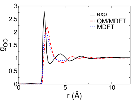
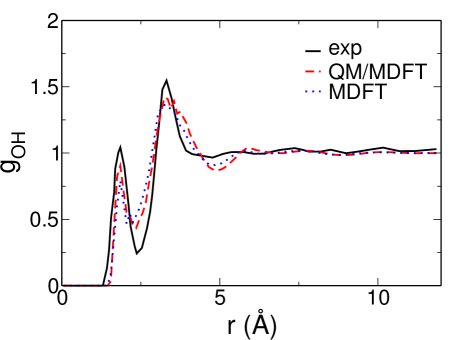
Figure 3: Radial distributions functions between the O site of the solvent and the O (top) or H (down) site of the solute. Results of the HNC functional for the classical SPC/E solute are in dotted blue while the one obtained with a QM solute are in dashed red. For comparison we reported the experimental results by Soper in full black (Soper, 2000).

While rdf function is a practical way to examine solvation structure it only contains spherically averaged information. This is not the case of the 3D densities that can be computed with MDFT. We estimate the solvent charge $\sigma_{\text{CSM}}$ using the CSM model implemented in GPAW (Held and Walter, 2014) and compare it to the 3D solvent charge density $\sigma_{\text{V}}$ given by equation 5. We assume that the whole difference between the electrostatic potential in CSM, $\Phi_{\text{CSM}}^{\text{ES}}$ and the one in vacuum $\Phi_{\text{vac}}^{\text{ES}}$ is due to the electrostatic potential generated by solvent $\Phi_{\text{V}}^{\text{ES}}$

$$\Phi_{\text{V}}^{\text{ES}}=\Phi_{\text{CSM}}^{\text{ES}}-\Phi_{\text{vac}}^{\text{ES}}.$$ (9)

This electrostatic potential $\Phi_{\text{V}}^{\text{ES}}$ is linked to the solvent charge $\sigma_{\text{CSM}}$ through a Poisson equation

$$\Delta\Phi_{\text{V}}^{\text{ES}}=-\frac{\sigma_{\text{CSM}}}{\epsilon_{0}}$$ (10)

where $\epsilon_{0}$ is the vacuum permitivitty.

Of course the charge density $\sigma_{\text{CSM}}$ actually does not solely contain the contribution due to the dielectric response of the solvent. The modification of the electronic density also impacts the electrostatic potential. Moreover, in equation 10 we simply used the vacuum permitivitty while we should have used the spatially varying permittivity entering the continuum model. Thus, the charge density $\sigma_{\text{CSM}}$ is simply a qualitative tool to visualise solvation effect in the CSM calculation.

In figure 4 we compare the charge densities obtained with CSM and with MDFT. The solvent charge density $\sigma_{\text{V}}$ predicted by MDFT is more structured than $\sigma_{\text{CSM}}$: there are additional lobes. To ease the discussion, we identify the lobes in figure 4 by their distance with respect to the centre of mass of the solute. The closest positive lobe is denoted $1^{+}$, the second negative $2^{-}$, etc.

The lobes $1^{+}$ and $1^{-}$ are similar in the CSM calculation and in the MDFT calculation. However, the charge distribution obtained by CSM is located on the cavity surface while the lobes obtained with MDFT have 3D shapes.

$1^{+}$ and $1^{-}$ correspond to the first solvation shell and not surprisingly we observe that the solvent is polarised such as positives charges appear close to the oxygen atom while negative charges develop close to the hydrogen atoms. In the MDFT results, a second set of lobes exist. They have a shape similar to the one of the first lobes but with opposite charge and they are located in their vicinity, e.g. $2^{+}$ is close to $1^{-}$. We estimated the distance between $1^{+}$ and $2^{-}$ and between $2^{+}$ and $1^{-}$ by measuring distances between several pairs of points pertaining to each isosurface. We found that both pairs of isosurfaces are roughly distant by $1\ \textrm{\r{A}}$. This is of the order of the OH bond length in the SPC/E water model, thus each pairs of oppositely charge isosurfaces belong to the first solvation shell of water. We recover the tetrahedral order with preferential orientation of water around the water solute molecule.

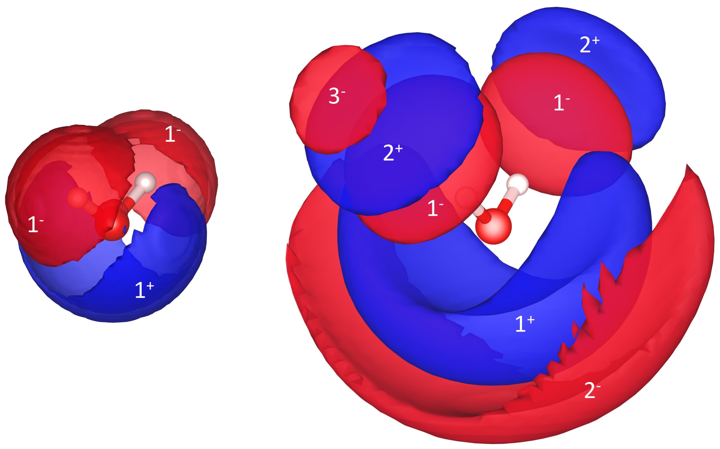
Figure 4: Isosurfaces of solvent charge densities: positive surfaces are displayed in blue and negative ones in red. The left figure have been obtained with the CSM calculation using equation 10. The right one have been obtained with MDFT with equation 5.

While the dipole moment of the water molecule is well known to be 1.85 D in the gas phase (Clough et al., 1973) its value in the liquid have been more controversial with simulation prediction ranging from 2.1 to 3.1 D (Gubskaya and Kusalik, 2002). In the beginning of the 2000’s several independent experimental studies have found a value of 2.9-3.0 D for the dipole moment in the liquid (Badyal et al., 2000; Gubskaya and Kusalik, 2002). In table 3 we display the dipole moment of a water molecule in gas and liquid phase. We obtain a dipole of 1.9 D with the PBE functional, in good agreement with the experimental value. The value in solution is estimated to 2.3 D with the continuum solvation model. This is clearly underestimated with respect to the experimental value but this falls within the range of values predicted using simulations and QM/MM approaches (Rocha et al., 2001). Note that this value is interestingly close to 2.35 D which is the one of the SPC/E model (Mark and Nilsson, 2001). With the MDFT approach we do obtain an enhancement of the dipole of the water molecule in solution. After a single MDFT calculation most of the polarisation is recovered with a dipole of 2.2 D. After converging the self consistent cycle, the dipole increases to 2.3 D. Once again, this shows the importance of the self consistent optimisation of electronic and solvent densities to account for their mutual polarisation.

Note that the same value of the dipole is obtained using any of the Lennard-Jones parameters of table 2. It should be noted that several AIMD simulations of liquid water using the PBE functional have found a dipole value of 2.9-3.2 D (Allesch et al., 2004; McGrath et al., 2007) which is in good agreement with experiments. The underestimation of the dipole moment in the liquid phase in the MDFT calculation may have several origin. First, it has been demonstrated using ab initio MD that the dipole moment of rigid water molecules tends to be smaller than when the geometry is allowed to relax (Allesch et al., 2004). Second, as opposed to AIMD there is no electronic polarisation of the solvent molecules since we use a non-polarisable model. A third reason might be the limitation of the HNC functional. As illustrated in figure 3, the first peak of the oxygen rdf is broaden, reduced and shifted further from the solute with the HNC functional with respect to experiments while the hydrogen rdf more or less agree. Consequently, the charge distribution of the solvent predicted by the HNC functional is smoother. As a consequence, the electric field generated by the solvent is reduced and the water solute is less polarised than in experiment.

$\mu$(D)	vacuum	solution
exp.	1.85	2.9-3.0
CSM	1.9	2.3
MDFT	1.9	2.3 (2.2)

Table 3: Molecular dipole of the water molecule in the gas phase and in the liquid. The vacuum value of 1.9 D correspond to a unique calculation. The value obtained with a QM calculation followed by a unique MDFT calculation is displayed in parenthesis.

As a conclusion, this study of water in water with the QM/MDFT approach is encouraging. We are able to recover the tetrahedral structure of the first solvation shell around the solute and the enhancement of the water dipole in the liquid phase. However, some defects of the HNC functional are still present. In particular the solvation shell is not structured enough. There is still room to improve the functional, a natural route being to introduce an appropriate bridge term. These defects should not obliviate the potential of the method due to its computational efficiency with respect to AIMD. It took 25 minutes on a 32 CPU desktop machine to carry the full self-consistent QM/MDFT cycle, computing the chemical potential of water using AIMD would require to use enhance sampling methods and take tens of thousands of CPU-hours. To further illustrate the interest of the approach, we now turn our attention to the prototypical symmetric $\text{S}{}_{\text{N}}2$ reaction between chloromethane and a chloride anion.

III.2 $\text{S}{}_{\text{N}}2$ reaction

Due to its extensive use as a tool to switch functional group in organic molecules, many experimental and theoretical studies have been dedicated to study the $\text{S}{}_{\text{N}}2$ reaction. Because the nucleophile is very often an anion, solvent effect can deeply modify the free energy profile of the reaction. Thus, a smart choice of solvent can modulate the reactivity and the selectivity of the reaction (Hughes and Ingold, 1935; Gertner et al., 1989; Ensing et al., 2001). This explains that many studies have been dedicated to investigate solvation effect in $\text{S}{}_{\text{N}}2$ reaction by simulation (Bento et al., 2008; Chandrasekhar et al., 1984, 1985; Gao and Xia, 1993; Ensing et al., 2001; Kuechler and York, 2014; Gertner et al., 1989; Tirado-Rives and Jorgensen, 2019; Zhao and Truhlar, 2010). In particular, QM/MM is a method of choice since it allows to account for bond breaking/formation between the nucleophile and the electrophile while keeping a realistic description of the solvent with a tractable numerical cost.

We examine the reaction free energy of the symmetrical $\text{S}{}_{\text{N}}2$ reaction between chloromethane and chloride in water. We chose the same reaction coordinate, $r,$ as many other studies (Chandrasekhar et al., 1984, 1985; Huston et al., 1989; Kuechler and York, 2014; Cai et al., 2019; Tirado-Rives and Jorgensen, 2019) that is the difference between the two carbon chlorine distances $r=\left|d_{\text{C-C$l_{1}$}}-d_{\text{C-C$l_{2}$}}\right|$. We first run the calculation in the gas phase using GPAW with the PBE functional and the partial wave basis. The simulation box is $24\times 24\times 24\ \textrm{\r{A}}^{3}$. We first identify the transition state (TS) of the molecule by running calculation on the $\text{$\left[\text{Cl}\text{\textemdash}\text{CH}_{3}\text{\textemdash}\text{Cl}\right]$}^{-}$ complex where chlorines and carbon atoms are collinear. Carbon and chlorine atoms are fixed with two identical carbon chlorine bond length while the positions of hydrogen atoms are allowed to relax. We vary the carbon chlorine distances to identify the most stable structure. In the transition state, the carbon chlorine distance is 2.33 Å and the hydrogen are located on the edges of an equilateral triangle perpendicular to the Cl—Cl axis, we recover the expected $D_{3}h$ symmetry for the TS. To compute the energy profile along the reaction coordinate we elongate the bond between the carbon and the first chlorine $\text{C}\text{l}_{1}$ and fix the positions of these two atoms. Other atoms are relaxed with the constraint of collinearity between carbon and the two chlorines. The energy profile in vacuum is displayed in figure 5, it exhibits a minimum between the TS and the dissociated state (DS) which correspond to a so-called ion-dipole complex (IDC). The structure parameters of TS, IDC and DS are given in table 4. These structures are in overall good agreement with the one reported by Cai et al (Cai et al., 2019) obtained using M06-2X/6-311++g. The only major difference is a slightly elongated distance between carbon and the less bounded chlorine in the IDC.

While the shape of the energy profile in vacuum is correct, the agreement with previous studies (Kuechler and York, 2014; Cai et al., 2019; Tirado-Rives and Jorgensen, 2019) is not quantitative. We obtain -29.7 kJ.mol^-1 for the energy difference between the DS and the IDC. In a recent benchmark, Tirado-Rives and collaborators have found a stabilisation of the IDC varying between $-36.0$ and $-51.9$ kJ.mol^-1 using various methods (Tirado-Rives and Jorgensen, 2019). We predict an energy barrier, i.e an energy difference between the TS and the IDC, of $31.3\$ kJ.mol^-1 while Bierbaum and coworkers have found a barrier of $55.2\pm 9$ kJ.mol^-1 using kinetic analysis (Barlow et al., 1988; DePuy et al., 1990). Kuechler and collaborators have tested a wide variety of methods to compute the energy barrier and they found an energy difference with respect to the experimental value up to -19.3 kJ.mol^-1 (Kuechler and York, 2014).

	dC-Cl1	dC-Cl2	dC-H	$\angle$HCH	$\angle$HCCl	$r\ \left(\textrm{\r{A}}\right)$
TS	2.33 Å	2.33 Å	1.08 Å	120$\textdegree$	90$\textdegree$	0
IDC	1.83 Å	3.33 Å	1.09 Å	110.7$\textdegree$	108.1$\textdegree$	1.3
DS	1.79 Å	N/A	1.09 Å	110.4$\textdegree$	108.4$\textdegree$	6.2

Table 4: Structure parameters of the transition state (TS), ion-dipole complex (IDC) and dissociated state (DS) in the gas phase.

To study the solvation effect on the symmetric $\text{S}{}_{\text{N}}2$ reaction we coupled the eDFT calculation above with an MDFT description of the SPC/E solvent. The electronic densities are computed for each geometry on a regular spatial grid made of $240\times 240\times 240$ nodes. The same space grid is used for MDFT with 196 possible orientations. We choose the same set of Lennard-Jones parameters as the one used by Gao and Xia (Gao and Xia, 1993) which are reminded in table 5. The eDFT and MDFT program are run sequentially until a convergence criterion of $10^{-3}$ is reached for both the relative change in energy for GPAW and in free energy for MDFT. We apply the usual periodic boundary condition corrections of charged solutes (Kastenholz and Hünenberger, 2006a, b) and the correction due to the pressure overestimation in HNC (Sergiievskyi et al., 2014). The solvation free energy computed using eDFT/MDFT is displayed in figure 5. The minimum corresponding to the IDC almost vanished while the free energy barrier increases considerably to 58.7 kJ.mol^-1. However, this value is still underestimated compared to the experimental value of 111 kJ.mol^-1 (Albery and Kreevoy, 1978). The increase of the free energy barrier can be split into two contributions, the first one being the polarisation of the solute by the solvent. It can be estimated by comparing the values of the in-vacuo electronic functional evaluated with the equilibrium electronic densities obtained in vacuum and in the presence of the solvent. This polarisation contribution decreases the free energy barrier by 5.9 kJ.mol^-1. The second and dominating contribution is the stabilisation by the solvent which increases the barrier by roughly 29 kJ.mol^-1.

The solvation free energy profile was also computed using the CSM implemented in GPAW (Held and Walter, 2014), it is displayed in figure 5. The free energy barrier is 70.3 kJ.mol^-1, a value that is also underestimated with respect to the experimental one.

The overall agreement of the eDFT/MDFT calculation may seems disappointing considering that some previous studies were more quantitative, even with semi-empirical model (Kuechler and York, 2014). However this work is the first attempt to self consistently optimise molecular and electronic functional. It is encouraging that the solvation effects are well reproduced, at least qualitatively. Moreover, the free energy profile is consistent with the prediction of the CSM.

There are several avenues to improve the results, first the electronic functional is clearly not appropriate to reproduce the gas phase predictions, the MO6-2X functional (Zhao and Truhlar, 2008) seems more suited for instance (Tirado-Rives and Jorgensen, 2019; Cai et al., 2019).

Second, the choice of the Lennard-Jones parameters may not be so innocent. This is particularly true in this $\text{S}{}_{\text{N}}2$ reaction where the chlorine atom is described with the same parameters if it is bonded or in its anionic state. This seems to be natural in QM/MM studies, for instance in previous studies using the OPLS-AA force field the parameters for chlorine in halogenoalkane (Jorgensen and Schyman, 2012) are used for all values of the reaction coordinate. It would probably be more correct to use a combination of the Lennard-Jones parameters of the chloride (Jensen and Jorgensen, 2006) and the chlorine in halogenoalkane depending on the value of the reaction coordinate, this is the object of current investigation. From the MDFT point of view we recover some known defects of the HNC functional and the SPC/E model, i.e. a missing bridge term for the former and no explicit treatment of water polarisability for the latter.

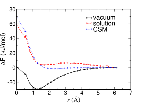
Figure 5: Potential of mean force of the $\text{S}{}_{\text{N}}2$ reaction as a function of the reaction coordinate. The calculation in vacuum is in full black and circles. The free energy in solution obtained with QM/MDFT are in dashed red with squares. The SFE obtained using the CSM implemented in GPAW is in dotted blue with diamonds.

	$\sigma\ (\textrm{\r{A}})$	$\epsilon\ (\text{kJ.mo$l^{-1}$})$
Cl	4.1964	0.4682
C	3.4000	0.4184
H	2.0000	0.29288

Table 5: Lennard-Jones parameters for symmetrical S${}_{\text{N}}$2 reaction in water.

Compared to continuum model a solid advantage of MDFT is its prediction of the solvent structure at the molecular level. Indeed, the equilibrium density $\rho(\bm{r},\bm{\Omega})$ contains a lot of information about the solvation structure. In particular, it is possible to follow the solvent reorientation during the removal of the nucleofuge. To do so, we compute the average orientation density $\bm{\bar{\Omega}}$ defined as

$$\bar{\bm{\Omega}}(\bm{r})=\frac{\int\rho(\bm{r},\bm{\Omega})\bm{\Omega}d\bm{\Omega}}{\int\rho(\bm{r},\bm{\Omega})d\bm{\Omega}}.$$ (11)

The direction of this vector gives the average orientation. Its norm gives the proportion of the average orientation with respect to other orientations. The average orientation density and the number density in a plane containing the carbon, the 2 chlorine and one hydrogen are displayed in figures 6-8 for the geometries of table 4. The average orientations are represented by vectors oriented from oxygen towards hydrogens which length are proportional to $\left\|\bm{\bar{\Omega}}\right\|$. To improve the readability of the figure, orientation are depicted on a grid twice as loose as the one used for calculation.

Water number densities and average orientation around the TS are symmetrical with respect to the plane containing the $\text{CH}{}_{3}$ fragment as displayed in figure 6. Concerning the number densities, we identify two high density shells separated by a region where the density is reduced compared to the bulk one. At every location in the second solvation shell the favoured orientation is the one with hydrogens pointing towards the solute. This is not surprising since the solute is globally negative, at this distance it is seen as a symmetric anion. However, other orientations are not insignificant as illustrated by the small size of the arrows. In the depletion region, there are no favoured orientations. In the first solvation shell, we first mention that the most marked orientation i.e the location denoted by the longest arrows are in the region the closest to the solute where the number density is almost zero. In this shell, the favoured orientation at any point are globally pointing towards the closest chlorine atom, except in a small region located close to the plane of the bisector of the Cl-Cl bond where the preferred orientation is pointing outward. Thus, the orientation in the first solvation shell is consistent with the usual charge picture of the transition state in which each chlorine is globally anionic and the CH₃ fragment is almost neutral (Tirado-Rives and Jorgensen, 2019; Cai et al., 2019; Kuechler and York, 2014).

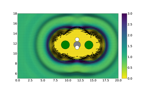
Figure 6: Average number density of water around the TS in the plane mentioned in the text. The high density region are in blue, the low density region are in yellow. The average orientation of the water molecule as computed by equation 11 are represented by arrows. Carbon atom is in grey, chlorine atoms are in green and hydrogen atoms are in white.

The number and average orientation densities around the structure corresponding to the IDC are displayed in figure 7. As compared to the TS, the number densities are not drastically modified. In the first solvation shell, the number density around the leaving chlorine is increased while the one around the bounded one is decreased. A similar effect is observed in the second solvation shell but it is less pronounced. The differences between the average orientations densities of the IC and the TS are more obvious. In the second solvation shell, the preferential orientation are still pointing towards the closest chlorine but the symmetry has clearly been broken. It looks like the superimposition of two spherical shells centred on each chlorine. The preferential orientation around the leaving chlorine is even more pronounced than in the TS while the one around the bounded one almost already recovered a bulk behaviour with no preferential orientation. A similar behaviour occurs in the first solvation shell which displays a decided average orientation around the leaving chlorine while the preferred orientations towards the bonded chlorine is still present but drastically reduced. These observations are consistent with an ionic complex. The two chlorines are anionic but the one the furthest from the carbon bears a more negative charge than the closest one.

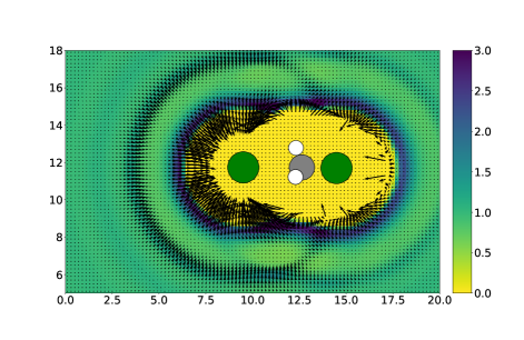
Figure 7: Same as figure 6 for the IDC.

In the dissociated state, displayed in figure 8 the number density and average orientation density follow a similar trend. The second shell around the chloromethane is no longer visible neither in number density nor in average orientation density. The two solvation shells around the leaving chlorine are spherical with a marked orientation pointing toward the nucleus which is consistent with an anion. The most interesting feature are observed in the first solvation shell of the chloromethane where the preferential orientation in the first solvation shell are pointing outwards the molecule. This is quite surprising since in the usual point charge model the chloromethane being described as a dipolar molecule the water molecule close to chlorine would point towards this atoms.

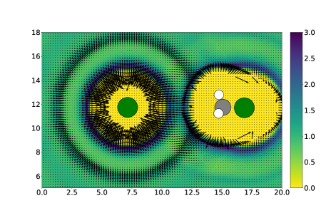
Figure 8: Same as figure 6 for the DS.

IV Conclusions

The introduced QM/MDFT approach is well suited to study solvation problems. It is particularly appropriate to compute solvation free energies and 3D molecular densities. QM/MDFT is based on the standard QM/MM approximation where the solute is described by quantum mechanics and solvent by molecular mechanics using ad hoc force fields. However, while the MM system is most often treated using Molecular Dynamics or Monte-Carlo we employ molecular density functional theory instead. It is no longer needed to generate extensive trajectory to compute free energy, this is the direct outcome of a much simpler functional minimisation. While any variational QM methods could be chosen in principle, electronic DFT is the most natural to be coupled with classical DFT (Petrosyan et al., 2005, 2007). With this choice, the solvation free energy can be computed doing a self consistent optimisation of the electronic and solvent functionals. This could be done simultaneously but the joint minimisation is done iteratively in this paper. This self consistent approach account for the mutual polarisation of the solvent and solute, a phenomena that is disregarded in previous attempt to couple eDFT and classical DFT (Cai et al., 2019; Tang et al., 2018).

To illustrate the possibilities of QM/MDFT we first studied the solvation of a quantum water molecule in a solvent of classical water. The water dipole is enhanced in the liquid as compared to the gas phase. This is encouraging but the value of the dipole is underestimated with respect to the experimental measurement. Unfortunately, describing the solute at the QM level does not fix the known flaws of the MDFT functional at the HNC level, especially on the solvation structure. The first peak of the radial distribution between the oxygen of the solute and the oxygen of the solvent is too broad and the second peak is misplaced. This calls for bridge functional improvement that are currently underway.

We then turn to the study of a symmetrical aqueous S${}_{\text{N}}$2 reaction between chloromethane and chloride. The free energy profiles are qualitatively correct, the local minimum observed in gas phase vanished in the liquid. We were also able to follow in detail the solvation structure around the reactants along the reaction coordinate. However, the quantitative agreement between the predicted solvation free energies and the experimental one is rather disappointing. There are several room for improvement. First, the electronic functional should be carefully chosen as different functional can predict energy barriers differing by several eV. Second, we should reexplore the corrections to the HNC molecular functional in the light of the QM/MM problem or better, complement the HNC functional by a well founded bridge term.

These points surely need to be explored to make the QM/MDFT method more robust to become a credible alternative to expansive AIMD or too simplistic continuum solvent models.

References

- Hughes and Ingold (1935) Edward D. Hughes and Christopher K. Ingold, “55. mechanism of substitution at a saturated carbon atom. part iv. a discussion of constitutional and solvent effects on the mechanism, kinetics, velocity, and orientation of substitution,” Jorunal of the Chemical Society , 244–255 (1935).
- Liu et al. (2018) Xu Liu, Jiaxu Zhang, Li Yang, and William L. Hase, “How a Solvent Molecule Affects Competing Elimination and Substitution Dynamics. Insight into Mechanism Evolution with Increased Solvation,” Journal of the American Chemical Society 140, 10995–11005 (2018).
- Han et al. (2016) You Han, Dandan Jiang, Jinli Zhang, Wei Li, Zhongxue Gan, and Junjie Gu, “Development, applications and challenges of ReaxFF reactive force field in molecular simulations,” Frontiers of Chemical Science and Engineering 10, 16–38 (2016).
- Senftle et al. (2016) Thomas P. Senftle, Sungwook Hong, Md Mahbubul Islam, Sudhir B. Kylasa, Yuanxia Zheng, Yun Kyung Shin, Chad Junkermeier, Roman Engel-Herbert, Michael J. Janik, Hasan Metin Aktulga, Toon Verstraelen, Ananth Grama, and Adri C. T. van Duin, “The ReaxFF reactive force-field: development, applications and future directions,” npj Computational Materials 2, 1–14 (2016).
- Frenkel and Smit (2002) Daan Frenkel and Berend Smit, Understanding molecular simulation: from algorithms to applications, second edition ed. (Academic Press, 2002).
- Silvestrelli and Parrinello (1999) Pier Luigi Silvestrelli and Michele Parrinello, “Water Molecule Dipole in the Gas and in the Liquid Phase,” Physical Review Letters 82, 3308–3311 (1999).
- Lin and Truhlar (2007) Hai Lin and Donald G. Truhlar, “QM/MM: what have we learned, where are we, and where do we go from here?” Theoretical Chemistry Accounts 117, 185 (2007).
- Tomasi and Persico (1994) Jacopo Tomasi and Maurizio Persico, “Molecular Interactions in Solution: An Overview of Methods Based on Continuous Distributions of the Solvent,” Chemical Reviews 94, 2027–2094 (1994).
- Tomasi et al. (2005) Jacopo Tomasi, Benedetta Mennucci, and Roberto Cammi, “Quantum Mechanical Continuum Solvation Models,” Chemical Reviews 105, 2999–3094 (2005).
- Klamt (2011) Andreas Klamt, “The COSMO and COSMO-RS solvation models,” Wiley Interdisciplinary Reviews: Computational Molecular Science 1, 699–709 (2011).
- Hansen and McDonald (2006) Jean-Pierre Hansen and I.R. McDonald, Theory of Simple Liquids, Third Edition, 3rd ed. (Academic Press, 2006).
- Chandler and Andersen (1972) David Chandler and Hans C. Andersen, “Optimized Cluster Expansions for Classical Fluids. II. Theory of Molecular Liquids,” The Journal of Chemical Physics 57, 1930–1937 (1972).
- Ebner et al. (1976) C. Ebner, W. F. Saam, and D. Stroud, “Density-functional theory of simple classical fluids. I. Surfaces,” Physical Review A 14, 2264–2273 (1976).
- Belloni and Chikina (2014) Luc Belloni and Ioulia Chikina, “Efficient full Newton-Raphson technique for the solution of molecular integral equations - example of the SPC/E water-like system,” Molecular Physics 112, 1246–1256 (2014).
- Ramirez et al. (2002) Rosa Ramirez, Ralph Gebauer, Michel Mareschal, and Daniel Borgis, “Density functional theory of solvation in a polar solvent: Extracting the functional from homogeneous solvent simulations,” Physical Review E 66, 031206–031206–8 (2002).
- Zhao et al. (2011) Shuangliang Zhao, Rosa Ramirez, Rodolphe Vuilleumier, and Daniel Borgis, “Molecular density functional theory of solvation: From polar solvents to water,” The Journal of Chemical Physics 134, 194102 (2011).
- Jeanmairet et al. (2013a) Guillaume Jeanmairet, Maximilien Levesque, and Daniel Borgis, “Molecular density functional theory of water describing hydrophobicity at short and long length scales,” The Journal of Chemical Physics 139, 154101–1–154101–9 (2013a).
- Jeanmairet et al. (2013b) Guillaume Jeanmairet, Maximilien Levesque, Rodolphe Vuilleumier, and Daniel Borgis, “Molecular Density Functional Theory of Water,” The Journal of Physical Chemistry Letters 4, 619–624 (2013b).
- Jeanmairet et al. (2015) Guillaume Jeanmairet, Maximilien Levesque, Volodymyr Sergiievskyi, and Daniel Borgis, “Molecular density functional theory for water with liquid-gas coexistence and correct pressure,” The Journal of Chemical Physics 142, 154112 (2015).
- Jeanmairet et al. (2016) Guillaume Jeanmairet, Nicolas Levy, Maximilien Levesque, and Daniel Borgis, “Molecular density functional theory of water including density-polarization coupling,” Journal of Physics: Condensed Matter 28, 244005 (2016).
- Jeanmairet et al. (2019a) Guillaume Jeanmairet, Benjamin Rotenberg, Daniel Borgis, and Mathieu Salanne, “Study of a water-graphene capacitor with molecular density functional theory,” The Journal of Chemical Physics 151, 124111 (2019a).
- Jeanmairet et al. (2019b) Guillaume Jeanmairet, Benjamin Rotenberg, Maximilien Levesque, Daniel Borgis, and Mathieu Salanne, “A molecular density functional theory approach to electron transfer reactions,” Chemical Science 10, 2130–2143 (2019b).
- Kovalenko and Hirata (1998) Andriy Kovalenko and Fumio Hirata, “Three-dimensional density profiles of water in contact with a solute of arbitrary shape: a RISM approach,” Chemical Physics Letters 290, 237–244 (1998).
- Ding et al. (2017) Lu Ding, Maximilien Levesque, Daniel Borgis, and Luc Belloni, “Efficient molecular density functional theory using generalized spherical harmonics expansions,” The Journal of Chemical Physics 147, 094107 (2017).
- Ten-no et al. (1993) Seiichiro Ten-no, Fumio Hirata, and Shigeki Kato, “A hybrid approach for the solvent effect on the electronic structure of a solute based on the RISM and Hartree-Fock equations,” Chemical Physics Letters 214, 391–396 (1993).
- Naka et al. (1999) Kazunari Naka, Hirofumi Sato, Akihiro Morita, Fumio Hirata, and Shigeki Kato, “RISM-SCF study of the free-energy profile of the Menshutkin-type reaction NH3+CH3ClNH3CH3++Cl- in aqueous solution,” Theoretical Chemistry Accounts 102, 165–169 (1999).
- Sato et al. (2000) Hirofumi Sato, Andriy Kovalenko, and Fumio Hirata, “Self-consistent field, ab initio molecular orbital and three-dimensional reference interaction site model study for solvation effect on carbon monoxide in aqueous solution,” The Journal of Chemical Physics 112, 9463–9468 (2000).
- Kasahara and Sato (2018) Kento Kasahara and Hirofumi Sato, “Solvation Structure of LiClO4/Ethylene Carbonate Solution near a Graphite Electrode in Lithium-ion Batteries: 3D-RISM Study,” Chemistry Letters 47, 311–314 (2018).
- Kaminski et al. (2010) Jakub W. Kaminski, Sergey Gusarov, Tomasz A. Wesolowski, and Andriy Kovalenko, “Modeling Solvatochromic Shifts Using the Orbital-Free Embedding Potential at Statistically Mechanically Averaged Solvent Density,” The Journal of Physical Chemistry A 114, 6082–6096 (2010).
- Zhou et al. (2011) Xiuwen Zhou, Jakub W. Kaminski, and Tomasz A. Wesolowski, “Multi-scale modelling of solvatochromic shifts from frozen-density embedding theory with non-uniform continuum model of the solvent: the coumarin 153 case,” Physical Chemistry Chemical Physics 13, 10565–10576 (2011).
- Gusarov et al. (2006) Sergey Gusarov, Tom Ziegler, and Andriy Kovalenko, “Self-Consistent Combination of the Three-Dimensional RISM Theory of Molecular Solvation with Analytical Gradients and the Amsterdam Density Functional Package,” The Journal of Physical Chemistry A 110, 6083–6090 (2006).
- Casanova et al. (2007) David Casanova, Sergey Gusarov, Andriy Kovalenko, and Tom Ziegler, “Evaluation of the SCF Combination of KS-DFT and 3D-RISM-KH; Solvation Effect on Conformational Equilibria, Tautomerization Energies, and Activation Barriers,” Journal of Chemical Theory and Computation 3, 458–476 (2007).
- Petrosyan et al. (2005) S. A. Petrosyan, A. A. Rigos, and T. A. Arias, “Joint Density-Functional Theory: Ab Initio Study of Cr2O3 Surface Chemistry in Solution,” The Journal of Physical Chemistry B 109, 15436–15444 (2005).
- Petrosyan et al. (2007) S. A. Petrosyan, Jean-Francois Briere, David Roundy, and T. A. Arias, “Joint density-functional theory for electronic structure of solvated systems,” Physical Review B 75, 205105 (2007).
- Sundararaman et al. (2017) Ravishankar Sundararaman, Kendra Letchworth-Weaver, Kathleen A. Schwarz, Deniz Gunceler, Yalcin Ozhabes, and T.A. Arias, “JDFTx: software for joint density-functional theory,” SoftwareX 6, 278–284 (2017).
- Sundararaman et al. (2012) Ravishankar Sundararaman, Kendra Letchworth-Weaver, and T. A. Arias, “A computationally efficacious free-energy functional for studies of inhomogeneous liquid water,” The Journal of Chemical Physics 137, 044107 (2012).
- Sundararaman and Arias (2014) Ravishankar Sundararaman and T. A. Arias, “Efficient classical density-functional theories of rigid-molecular fluids and a simplified free energy functional for liquid water,” Computer Physics Communications 185, 818–825 (2014).
- Tang et al. (2018) Weiqiang Tang, Cheng Cai, Shuangliang Zhao, and Honglai Liu, “Development of Reaction Density Functional Theory and Its Application to Glycine Tautomerization Reaction in Aqueous Solution,” The Journal of Physical Chemistry C 122, 20745–20754 (2018).
- Cai et al. (2019) Cheng Cai, Weiqiang Tang, Chongzhi Qiao, Peng Jiang, Changjie Lu, Shuangliang Zhao, and Honglai Liu, “A reaction density functional theory study of the solvent effect in prototype S N 2 reactions in aqueous solution,” Physical Chemistry Chemical Physics (2019).
- Tang et al. (2020) Weiqiang Tang, Jihao Zhao, Peng Jiang, Xiaofei Xu, Shuangliang Zhao, and Zhangfa Tong, “Solvent Effects on the Symmetric and Asymmetric SN2 Reactions in Acetonitrile Solution: A Reaction Density Functional Theory Study,” The Journal of Physical Chemistry B (2020).
- Sigfridsson and Ryde (1998) Emma Sigfridsson and Ulf Ryde, “Comparison of methods for deriving atomic charges from the electrostatic potential and moments,” Journal of Computational Chemistry 19, 377–395 (1998).
- Marenich et al. (2012) Aleksandr V. Marenich, Steven V. Jerome, Christopher J. Cramer, and Donald G. Truhlar, “Charge Model 5: An Extension of Hirshfeld Population Analysis for the Accurate Description of Molecular Interactions in Gaseous and Condensed Phases,” Journal of Chemical Theory and Computation 8, 527–541 (2012).
- Hu et al. (2007) Hao Hu, Zhenyu Lu, and Weitao Yang, “Fitting Molecular Electrostatic Potentials from Quantum Mechanical Calculations,” Journal of Chemical Theory and Computation 3, 1004–1013 (2007).
- Borgis et al. (2012) Daniel Borgis, Lionel Gendre, and Rosa Ramirez, “Molecular Density Functional Theory: Application to Solvation and Electron-Transfer Thermodynamics in Polar Solvents,” The Journal of Physical Chemistry B 116, 2504–2512 (2012).
- Evans (1979) R. Evans, “The nature of the liquid-vapour interface and other topics in the statistical mechanics of non-uniform, classical fluids,” Advances in Physics 28, 143 (1979).
- Levesque et al. (2012) Maximilien Levesque, Virginie Marry, Benjamin Rotenberg, Guillaume Jeanmairet, Rodolphe Vuilleumier, and Daniel Borgis, “Solvation of complex surfaces via molecular density functional theory,” The Journal of Chemical Physics 137, 224107–224107–8 (2012).
- Hohenberg and Kohn (1964) P. Hohenberg and W. Kohn, “Inhomogeneous Electron Gas,” Physical Review 136, B864 (1964).
- Tirado-Rives and Jorgensen (2019) Julian Tirado-Rives and William L. Jorgensen, “QM/MM Calculations for the Cl- + CH3Cl SN2 Reaction in Water Using CM5 Charges and Density Functional Theory,” The Journal of Physical Chemistry A 123, 5713–5717 (2019).
- Riccardi et al. (2004) Demian Riccardi, Guohui Li, and Qiang Cui, “Importance of van der Waals Interactions in QM/MM Simulations,” The Journal of Physical Chemistry B 108, 6467–6478 (2004).
- Tu and Laaksonen (1999) Yaoquan Tu and Aatto Laaksonen, “On the effect of Lennard-Jones parameters on the quantum mechanical and molecular mechanical coupling in a hybrid molecular dynamics simulation of liquid water,” The Journal of Chemical Physics 111, 7519–7525 (1999).
- Vaidehi et al. (1992) Nagarajan Vaidehi, Tomasz Adam Wesolowski, and Arieh Warshel, “Quantum-mechanical calculations of solvation free energies. A combined ab initio pseudopotential free-energy perturbation approach,” The Journal of Chemical Physics 97, 4264–4271 (1992).
- Schnitker and Rossky (1987) Jürgen Schnitker and Peter J. Rossky, “An electron-water pseudopotential for condensed phase simulation,” The Journal of Chemical Physics 86, 3462–3470 (1987), publisher: American Institute of Physics.
- Turi and Borgis (2002) László Turi and Daniel Borgis, “Analytical investigations of an electron-water molecule pseudopotential. II. Development of a new pair potential and molecular dynamics simulations,” The Journal of Chemical Physics 117, 6186–6195 (2002).
- Mones and Turi (2010) Letif Mones and László Turi, “A new electron-methanol molecule pseudopotential and its application for the solvated electron in methanol,” The Journal of Chemical Physics 132, 154507 (2010), publisher: American Institute of Physics.
- Sifain et al. (2018) Andrew E. Sifain, Nicholas Lubbers, Benjamin T. Nebgen, Justin S. Smith, Andrey Y. Lokhov, Olexandr Isayev, Adrian E. Roitberg, Kipton Barros, and Sergei Tretiak, “Discovering a Transferable Charge Assignment Model Using Machine Learning,” The Journal of Physical Chemistry Letters 9, 4495–4501 (2018).
- Enkovaara et al. (2010) J Enkovaara, C Rostgaard, J J Mortensen, J Chen, M Dułak, L Ferrighi, J Gavnholt, C Glinsvad, V Haikola, H A Hansen, H H Kristoffersen, M Kuisma, A H Larsen, L Lehtovaara, M Ljungberg, O Lopez-Acevedo, P G Moses, J Ojanen, T Olsen, V Petzold, N A Romero, J Stausholm-Møller, M Strange, G A Tritsaris, M Vanin, M Walter, B Hammer, H Häkkinen, G K H Madsen, R M Nieminen, J K Nørskov, M Puska, T T Rantala, J Schiøtz, K S Thygesen, and K W Jacobsen, “Electronic structure calculations with GPAW: a real-space implementation of the projector augmented-wave method,” Journal of Physics: Condensed Matter 22, 253202 (2010).
- Larsen et al. (2017) Ask Hjorth Larsen, Jens Jørgen Mortensen, Jakob Blomqvist, Ivano E Castelli, Rune Christensen, Marcin Dułak, Jesper Friis, Michael N Groves, Bjørk Hammer, Cory Hargus, Eric D Hermes, Paul C Jennings, Peter Bjerre Jensen, James Kermode, John R Kitchin, Esben Leonhard Kolsbjerg, Joseph Kubal, Kristen Kaasbjerg, Steen Lysgaard, Jón Bergmann Maronsson, Tristan Maxson, Thomas Olsen, Lars Pastewka, Andrew Peterson, Carsten Rostgaard, Jakob Schiøtz, Ole Schütt, Mikkel Strange, Kristian S Thygesen, Tejs Vegge, Lasse Vilhelmsen, Michael Walter, Zhenhua Zeng, and Karsten W Jacobsen, “The atomic simulation environment—a python library for working with atoms,” Journal of Physics: Condensed Matter 29, 273002 (2017).
- Mortensen et al. (2005) J. J. Mortensen, L. B. Hansen, and K. W. Jacobsen, “Real-space grid implementation of the projector augmented wave method,” Phys. Rev. B 71, 035109 (2005).
- Ten-no et al. (1994) Seiichiro Ten-no, Fumio Hirata, and Shigeki Kato, “Reference interaction site model self-consistent field study for solvation effect on carbonyl compounds in aqueous solution,” The Journal of Chemical Physics 100, 7443–7453 (1994).
- Held and Walter (2014) Alexander Held and Michael Walter, “Simplified continuum solvent model with a smooth cavity based on volumetric data,” The Journal of Chemical Physics 141, 174108 (2014).
- Luukkonen et al. (2020) Sohvi Luukkonen, Maximilien Levesque, Luc Belloni, and Daniel Borgis, “Hydration free energies and solvation structures with molecular density functional theory in the hypernetted chain approximation,” The Journal of Chemical Physics 152, 064110 (2020).
- Soper (2000) A. K. Soper, “The radial distribution functions of water and ice from 220 to 673 K and at pressures up to 400 MPa,” Chemical Physics 258, 121–137 (2000).
- Mark and Nilsson (2001) Pekka Mark and Lennart Nilsson, “Structure and Dynamics of the TIP3P, SPC, and SPC/E Water Models at 298 K,” The Journal of Physical Chemistry A 105, 9954–9960 (2001).
- Clough et al. (1973) Shepard A. Clough, Yardley Beers, Gerald P. Klein, and Laurence S. Rothman, “Dipole moment of water from Stark measurements of H2O, HDO, and D2O,” The Journal of Chemical Physics 59, 2254–2259 (1973).
- Gubskaya and Kusalik (2002) Anna V. Gubskaya and Peter G. Kusalik, “The total molecular dipole moment for liquid water,” The Journal of Chemical Physics 117, 5290–5302 (2002).
- Badyal et al. (2000) Y. S. Badyal, M.-L. Saboungi, D. L. Price, S. D. Shastri, D. R. Haeffner, and A. K. Soper, “Electron distribution in water,” The Journal of Chemical Physics 112, 9206–9208 (2000).
- Rocha et al. (2001) Willian R. Rocha, Kaline Coutinho, Wagner B. de Almeida, and Sylvio Canuto, “An efficient quantum mechanical/molecular mechanics Monte Carlo simulation of liquid water,” Chemical Physics Letters 335, 127–133 (2001).
- Allesch et al. (2004) Markus Allesch, Eric Schwegler, François Gygi, and Giulia Galli, “A first principles simulation of rigid water,” The Journal of Chemical Physics 120, 5192–5198 (2004).
- McGrath et al. (2007) M. J. McGrath, J. I. Siepmann, I.-F. W. Kuo, and C. J. Mundy, “Spatial correlation of dipole fluctuations in liquid water,” Molecular Physics 105, 1411–1417 (2007).
- Gertner et al. (1989) Bradley J. Gertner, Kent R. Wilson, and James T. Hynes, “Nonequilibrium solvation effects on reaction rates for model SN2 reactions in water,” The Journal of Chemical Physics 90, 3537–3558 (1989).
- Ensing et al. (2001) Bernd Ensing, Evert Jan Meijer, P. E. Blöchl, and Evert Jan Baerends, “Solvation Effects on the SN2 Reaction between CH3Cl and Cl- in Water,” The Journal of Physical Chemistry A 105, 3300–3310 (2001).
- Bento et al. (2008) A. PatrÃcia Bento, Miquel Solà, and F. Matthias Bickelhaupt, “E2 and SN2 Reactions of X- + CH3CH2X (X = F, Cl); an ab Initio and DFT Benchmark Study,” Journal of Chemical Theory and Computation 4, 929–940 (2008).
- Chandrasekhar et al. (1984) Jayaraman Chandrasekhar, Scott F. Smith, and William L. Jorgensen, “SN2 reaction profiles in the gas phase and aqueous solution,” Journal of the American Chemical Society 106, 3049–3050 (1984).
- Chandrasekhar et al. (1985) Jayaraman Chandrasekhar, Scott F. Smith, and William L. Jorgensen, “Theoretical examination of the SN2 reaction involving chloride ion and methyl chloride in the gas phase and aqueous solution,” Journal of the American Chemical Society 107, 154–163 (1985).
- Gao and Xia (1993) Jiali Gao and Xinfu Xia, “A two-dimensional energy surface for a type II SN2 reaction in aqueous solution,” Journal of the American Chemical Society 115, 9667–9675 (1993).
- Kuechler and York (2014) Erich R. Kuechler and Darrin M. York, “Quantum mechanical study of solvent effects in a prototype SN2 reaction in solution: Cl- attack on CH3Cl,” The Journal of Chemical Physics 140, 054109 (2014).
- Zhao and Truhlar (2010) Yan Zhao and Donald G. Truhlar, “Density Functional Calculations of E2 and SN2 Reactions: Effects of the Choice of Density Functional, Basis Set, and Self-Consistent Iterations,” Journal of Chemical Theory and Computation 6, 1104–1108 (2010).
- Huston et al. (1989) Shawn E. Huston, Peter J. Rossky, and Dominic A. Zichi, “Hydration effects on SN2 reactions: an integral equation study of free energy surfaces and corrections to transition-state theory,” Journal of the American Chemical Society 111, 5680–5687 (1989).
- Barlow et al. (1988) Stephan E. Barlow, Jane M. Van Doren, and Veronica M. Bierbaum, “The gas phase displacement reaction of chloride ion with methyl chloride as a function of kinetic energy,” Journal of the American Chemical Society 110, 7240–7242 (1988).
- DePuy et al. (1990) Charles H. DePuy, Scott Gronert, Amy Mullin, and Veronica M. Bierbaum, “Gas-phase SN2 and E2 reactions of alkyl halides,” Journal of the American Chemical Society 112, 8650–8655 (1990).
- Kastenholz and Hünenberger (2006a) M. A. Kastenholz and Philippe H. Hünenberger, “Computation of methodology-independent ionic solvation free energies from molecular simulations. I. The electrostatic potential in molecular liquids,” The Journal of Chemical Physics 124, 124106 (2006a).
- Kastenholz and Hünenberger (2006b) Mika A. Kastenholz and Philippe H. Hünenberger, “Computation of methodology-independent ionic solvation free energies from molecular simulations. II. The hydration free energy of the sodium cation,” The Journal of Chemical Physics 124, 224501 (2006b).
- Sergiievskyi et al. (2014) Volodymyr P. Sergiievskyi, Guillaume Jeanmairet, Maximilien Levesque, and Daniel Borgis, “Fast Computation of Solvation Free Energies with Molecular Density Functional Theory: Thermodynamic-Ensemble Partial Molar Volume Corrections,” The Journal of Physical Chemistry Letters 5, 1935–1942 (2014).
- Albery and Kreevoy (1978) W. John Albery and Maurice M. Kreevoy, “Methyl Transfer Reactions,” in Advances in Physical Organic Chemistry, Vol. 16, edited by V. Gold and D. Bethell (Academic Press, 1978) pp. 87–157.
- Zhao and Truhlar (2008) Yan Zhao and Donald G. Truhlar, “The M06 suite of density functionals for main group thermochemistry, thermochemical kinetics, noncovalent interactions, excited states, and transition elements: two new functionals and systematic testing of four M06-class functionals and 12 other functionals,” Theoretical Chemistry Accounts 120, 215–241 (2008).
- Jorgensen and Schyman (2012) William L. Jorgensen and Patric Schyman, “Treatment of Halogen Bonding in the OPLS-AA Force Field: Application to Potent Anti-HIV Agents,” Journal of Chemical Theory and Computation 8, 3895–3901 (2012).
- Jensen and Jorgensen (2006) KP Jensen and WL Jorgensen, “Halide, ammonium, and alkali metal ion parameters for modeling aqueous solutions,” Journal of Chemical Theory and 2, 1499–1509 (2006).