A Monte Carlo comparison between template-based and Wiener-filter CMB dipole estimators

We review and compare two different CMB dipole estimators discussed in the literature, and assess their performances through Monte Carlo simulations. The first method amounts to simple template regression with partial sky data, while the second method is an optimal Wiener filter (or Gibbs sampling) implementation. The main difference between the two methods is that the latter approach takes into account correlations with higher-order CMB temperature fluctuations that arise from non-orthogonal spherical harmonics on an incomplete sky, which for recent CMB data sets (such as Planck) is the dominant source of uncertainty. For an accepted sky fraction of 81 % and an angular CMB power spectrum corresponding to the best-fit Planck 2018 $\Lambda$CDM model, we find that the uncertainty on the recovered dipole amplitude is about six times smaller for the Wiener filter approach than for the template approach, corresponding to 0.5 and 3  $\mu$K, respectively. Similar relative differences are found for the corresponding directional parameters and other sky fractions. We note that the Wiener filter algorithm is generally applicable to any dipole estimation problem on an incomplete sky, as long as a statistical and computationally tractable model is available for the unmasked higher-order fluctuations. The methodology described in this paper forms the numerical basis for the most recent determination of the CMB solar dipole from Planck, as summarized by Planck Collaboration (2020).

1 Introduction

The cosmic microwave background (CMB) radiation was discovered in 1965 by Penzias & Wilson (1965), and has ever since been the primary target for several dozens of CMB experiments. The main scientific target for most of these studies has been small variations in intensity and polarization that correspond to cosmic density variations some 380 000 years after the Big Bang. These variations contain a wealth of information about the early history and evolution of the universe; for a recent analysis, see, e.g., Planck Collaboration VI (2018).

The CMB sky features three main physical components. The first is simply a constant blackbody term with a temperature of 2.7255 K (Fixsen 2009), corresponding to the average temperature of the CMB photons populating the universe today. This component is often denoted the CMB monopole, acknowledging its correspondence to the lowest multipole moment in spherical harmonics space.

The second component is the CMB dipole, which has an amplitude of about 3 mK (Lineweaver 1997). The CMB dipole is the result of Doppler boosting caused by the motion of the measuring instrument with respect to the CMB rest frame. It may be decomposed into two components, namely the solar dipole caused by the movement of the solar system around the Milky Way’s center, and the orbital dipole generated by the movement of the Earth and the instrument around the Sun. Both components play an important role for CMB experiments, as they represent the best available astrophysical calibration source for most experiments. Specifically, the orbital dipole serves as an invaluable tool for absolute calibration, since the Earth–Sun distance and the orbital period are known with very high precision. Likewise, the solar dipole provides an excellent relative calibration target, since it is brighter than most other signals, has a perfectly known frequency spectrum, and is visible across the entire sky.

The third component is the CMB density fluctuations with typical variations of about 100 $\mu$K. These correspond very closely to a statistically isotropic and Gaussian random field with an angular power spectrum described by a $\Lambda$CDM power spectrum (Planck Collaboration VI 2018; Planck Collaboration VII 2018). In addition to these CMB sources, real-world microwave observations also contain contributions from astrophysical foregrounds, most notably in the form of synchrotron, free-free, spinning and thermal dust, and CO emission from the Milky Way (e.g., Planck Collaboration IV 2018).

This paper will discuss how to optimally estimate the amplitude and direction of the CMB dipole with data that contains both astrophysical foregrounds and small-scale CMB fluctuations. Obtaining robust estimates for these parameters is important for several reasons. First, since the CMB dipole is used as a calibration source for most experiments, a potential bias in the CMB dipole amplitude translates directly into a corresponding bias of the overall normalization of the angular CMB power spectrum. Second, because the CMB dipole is about four orders of magnitude brighter than the cosmological variations in the large-scale polarization field, it is necessary to estimate the relative gains between detectors within a single frequency channel prior to mapmaking with a precision better than $\mathcal{O}(10^{-4})$ in order to avoid significant bias on the optical depth of reionization, $\tau$ (Planck Collaboration VI 2018).

Uncertainties on the dipole parameters result mainly from four different contributors. First, statistical instrumental noise defines a fundamental floor for the overall sensitivity that can be achieved. Second, many systematic effects due to non-idealities in the instrument itself can induce spurious dipoles, including sidelobe pickup, time-variable gain, or ADC corrections. Third, as already mentioned, foreground emission from the Milky Way obscures our view of the CMB, and also carries a dipole moment. To mitigate this effect it is in practice necessary to mask out parts of the Galactic regions. However, working with incomplete sky coverage has the unwanted effect of making the spherical harmonic base functions, $Y_{\ell m}\left(\theta,\phi\right)$, lose their orthogonality. This leads to the fourth and last contaminant, which is confusion from the higher-order CMB temperature fluctuations when analysing partial-sky observations.

The traditional way of CMB dipole parameter estimation with real data has typically followed a fairly simple approach. First, the orbital dipole contribution is removed from the time-ordered data of a given experiment, which are subsequently co-added into pixelized sky maps. Then foreground contamination is suppressed either through some component separation technique or by simple template regression with respect to known foreground tracers. Next, some part of the sky is removed by masking, before finally the CMB dipole is estimated through template fitting with partial-sky and foreground-cleaned data, typically adopting the templates shown in Fig. 1. (Note that the monopole is usually included in the fit for marginalization purposes only, to avoid potential inaccuracies in the zero-level determination from biasing the dipole fit.) For one specific example of such an implementation, see, e.g., Planck Collaboration II (2016).

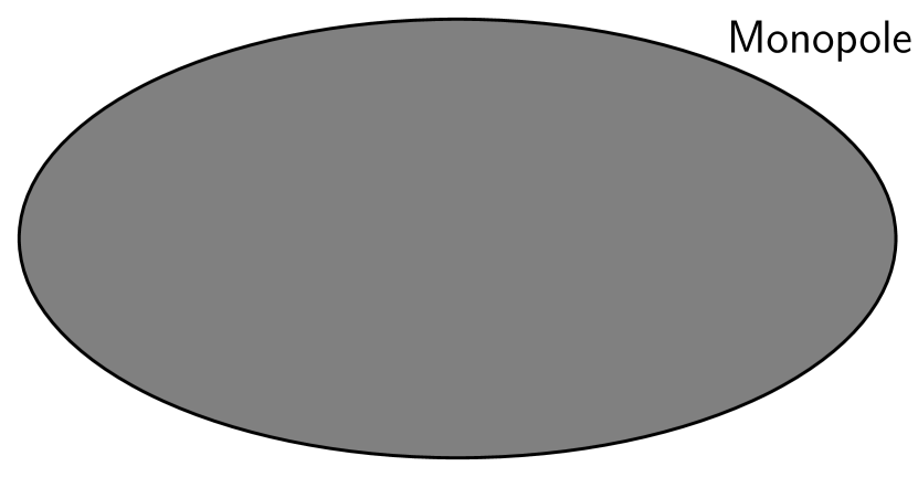
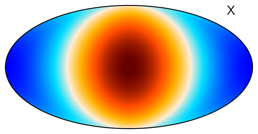
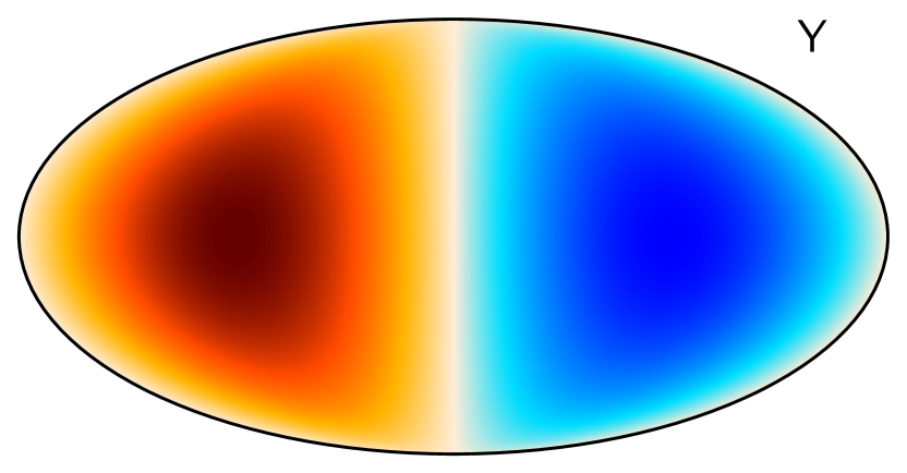
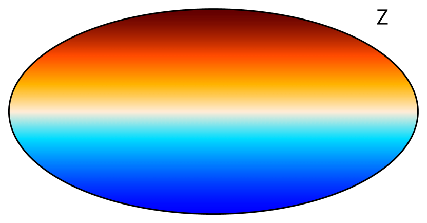
Figure 1: Basic templates used for CMB dipole estimation in the traditional template fitting approach. These correspond to the monopole (upper left) and the $x$- (upper right), $y$- (lower left), and $z$-dipoles (lower right).

As instrumental sensitivity has improved through the years, the specific details of each step in this procedure have become more important. For instance, for COBE-FIRAS (Fixsen et al. 1994) the uncertainty on the dipole amplitude due to statistical noise was 6 $\mu$K, while the foreground-induced uncertainty was about 14 $\mu$K. For comparison, Lineweaver (1997) estimated that the uncertainty due to confusion from higher-order CMB fluctuations was 3 $\mu$K, and this particular term was therefore irrelevant for COBE.

The same did not hold true for the Wilkinson Microwave Anisotropy Probe (WMAP) experiment, for which both the raw sensitivity and foreground rejection capabilities improved massively with respect to COBE. For this reason, the WMAP team replaced the simple dipole template-fitting procedure discussed above with a more sophisticated and optimal Wiener filter method (Hinshaw et al. 2009) originally pioneered by Jewell et al. (2004); Wandelt et al. (2004); Eriksen et al. (2004). The main advantage of this approach is the fact that the higher-order CMB fluctuations are estimated jointly with the dipole parameters, and by assuming that these correspond to a statistically isotropic and Gaussian random field, it is possible to partially reconstruct their properties even inside the Galactic mask.

The main goal of the current paper is to quantify the relative performance of the template fitting and Wiener filter methods. This has recently become a particularly important topic in the context of the Planck experiment, for which the sensitivity and control of systematic effects is so high that the total error budget has now become dominated by the higher-order CMB contribution. Specifically, the total instrumental uncertainty on the dipole amplitude is about 1 $\mu$K (Planck Collaboration I 2018), whereas the CMB confusion term arising from the naive template approach is, as we will see, typically between 1 and 3 $\mu$K, depending on sky fraction. Minimizing this term is therefore critically important. The results we obtain when applying this analysis framework to the latest Planck observations are summarized in Planck Collaboration (2020).

The rest of this paper is organized as follows: In Sec. 2 we give a short theoretical introduction on how the dipole parameters are obtained from sky maps, what effect partial sky coverage has on the uncertainties of these parameters, and further present a Wiener filter method for the estimation of these uncertainties. In Sec. 3 we describe the implementation of the uncertainty estimation technique. We present our results in Sec. 4, and we give our conclusions in Sec. 5.

2 Notation and methods

We start our discussion with a review of the traditional approach for estimating the dipole parameters (amplitude $A$, galactic longitude $l$ and latitude $b$) from a CMB map, and a discussion of how partial sky coverage complicates this procedure.

In this paper, we take as a starting point for dipole parameter estimation a cleaned CMB map in which as much foreground emission as possible has been removed; for details on how to perform foreground cleaning, we refer the interested reader to, e.g., Planck Collaboration IV (2018) and references therein. However, no component separation technique allows for perfect foreground removal, and there will always be some residual emission, especially in the galactic plane. One therefore must typically apply a mask to eliminate heavily contaminated regions on the sky. How to optimally estimate the dipole parameters from such a clean but incomplete CMB map is the main topic of this section.

2.1 Traditional template fitting

As a starting point for our analysis, we assume that the clean sky map may be written in the form

$$\@vec{d}=\@tens{T}\@vec{a}+\@vec{n},$$ (1)

where $\@tens{T}$ is a matrix containing the monopole and dipole templates in its columns, shown in Fig. 1; $\@vec{a}$ is a corresponding vector of template amplitudes; and $\@vec{n}$ is noise. Note that the latter may or may not include higher-order CMB fluctuations. In addition, we define a noise covariance matrix $\@tens{N}=\left<\@vec{n}\@vec{n}^{t}\right>$, and a diagonal mask matrix $\@tens{M}$ that is zero for masked pixels and unity for unmasked pixels.

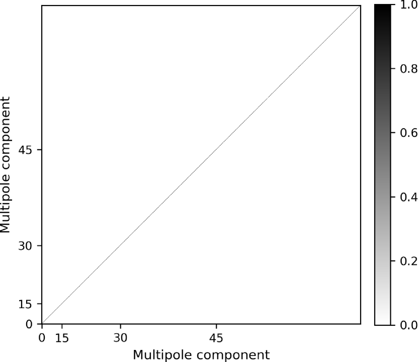
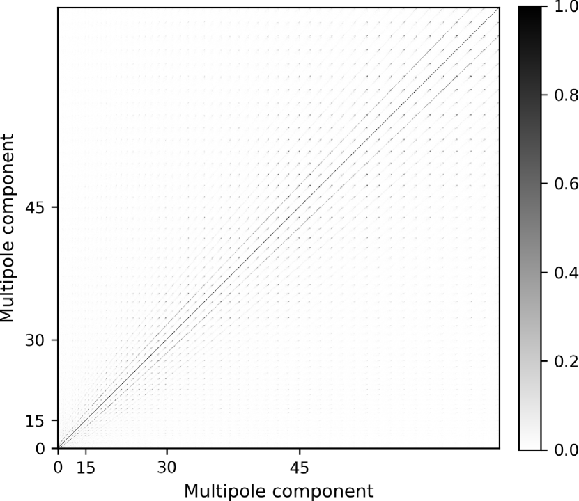
Figure 2: Spherical harmonics coupling kernel $K$ for $\ell\leq 60$ for an unmasked (top) and a masked (bottom) sky. Multipole moments are listed in $\ell$-major ordering with element numbering given by $i=\ell^{2}+\ell+m+1$. The sky fraction for the masked case is 36 %.

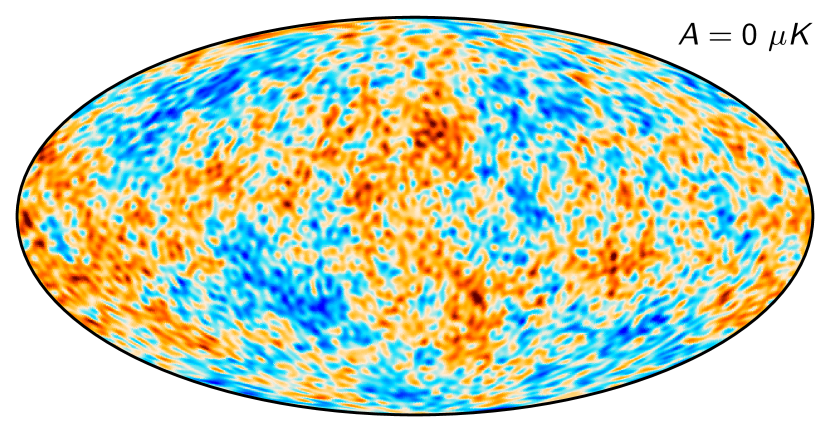
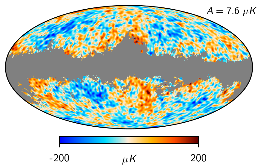
Figure 3: Illustration of spurious dipole excited from higher-order moments through mask coupling. The top panel shows an ideal CMB sky with identically vanishing dipole moment. The bottom panel shows the same realization, but with the Galactic plane masked. By accident, one large extended hotspot happens to lie on the western hemisphere inside the mask. Once this is removed by the mask, the net unmasked result is a dipole pointing toward the Eastern hemisphere with an amplitude of 7.6 $\mu$K.

Assuming that the noise is Gaussian, the maximum-likelihood solution for $\@vec{a}$ is then given by the so-called “normal equations”,

$$\@vec{a}={\left(\@tens{T}^{t}\@tens{M}\@tens{N}^{-1}\@tens{T}\right)}^{-1}\@tens{T}^{t}\@tens{M}\@tens{N}^{-1}\@vec{d}.$$ (2)

The trigonometric relations between these amplitudes and the dipole parameters are

$$A =\sqrt{a_{x}^{2}+a_{y}^{2}+a_{z}^{2}}$$ (3)

$$l =\arctan(a_{y}/a_{x})$$ (4)

$$b =90-\arccos(a_{z}/A).$$ (5)

Here, $a_{x}$, $a_{y}$ and $a_{z}$ are the components of the coefficient vector $\@vec{a}$ and $A$, $l$ and $b$ are the dipole amplitude, longitude and latitude respectively. Note that many commonly used implementations of this approach do not implement full inverse variance noise weighting, as described by Eq. 2, but simply adopt $\@tens{N}=\mathds{1}$, and thereby in effect assign equal weight to all pixels. We will do the same in the following.

2.2 Complications from partial sky coverage

The dipole parameters in Eq. 3–5 are subject to confusion from small-scale CMB fluctuations whenever a mask is applied. To see this, we expand the CMB fluctuation field into spherical harmonics as follows,

$$T\left(\hat{n}\right)=\sum_{\ell=0}^{\ell_{max}}\sum_{m=-\ell}^{\ell}a_{\ell m}Y_{\ell m}\left(\hat{n}\right),$$ (6)

where $T$ is the CMB fluctuation map; $Y_{\ell m}$ are the spherical harmonic base functions; and the $a_{\ell m}$ are the associated weights. With access to the full celestial sphere, these coefficients may be computed as

$$a_{\ell m}=\int_{4\pi}T\left(\hat{n}\right)Y_{\ell m}^{*}\left(\hat{n}\right)d\Omega.$$ (7)

However, when masking parts of the sky with a mask $\@tens{M}$ the spherical harmonic base functions are no longer orthogonal, and the new so-called pseudo-harmonic coefficients read (Hivon et al. 2002)

$$\begin{split}\tilde{a}_{\ell m}&=\int_{4\pi}\@tens{M}T\left(\hat{n}\right)Y_{\ell m}^{*}\left(\hat{n}\right)d\Omega\\ &=\sum_{\ell^{{}^{\prime}}m^{{}^{\prime}}}a_{\ell^{{}^{\prime}}m^{{}^{\prime}}}K_{\ell m,\ell^{{}^{\prime}}m^{{}^{\prime}}}\left[\@tens{M}\right].\end{split}$$ (8)

Here, $K$ is called the coupling kernel, and quantifies the mutual dependence between any two modes $Y_{\ell m}$ and $Y_{\ell^{\prime}m^{\prime}}$. The explicit expression for the coupling kernel reads

$$K_{\ell m,\ell^{{}^{\prime}}m^{{}^{\prime}}}=\int_{4\pi}\@tens{M}\left(\hat{n}\right)Y_{\ell m}\left(\hat{n}\right)Y_{\ell^{{}^{\prime}}m^{{}^{\prime}}}^{*}\left(\hat{n}\right)d\Omega.$$ (9)

Figure 2 shows $K$ for multipoles up to $\ell_{\text{max}}=60$ for two different cases. In the no-mask case, shown in the top panel, all modes are orthogonal and therefore independent. When we apply a mask, shown in the bottom panel, non-zero off-diagonal elements appear. In other words, any higher-order mode will induce a spurious dipole contribution unless properly accounted for.

Figure 3 provides an intuitive illustration of this effect. The top panel shows an ideal CMB realization drawn from a $\Lambda$CDM power spectrum with an identically vanishing dipole moment, $A=0$. However, one of the largest hotspots on the sky happens, by chance, to align closely with the western half of the Galactic plane. After applying the Galactic mask, which gives this hotspot zero weight in the dipole fit, the result is a net dipole that points in the opposite direction. In this particular case, the result is a spurious dipole of $7.6\thinspace\mu$K pointing towards the eastern hemisphere.

2.3 Wiener filtering and Gibbs sampling

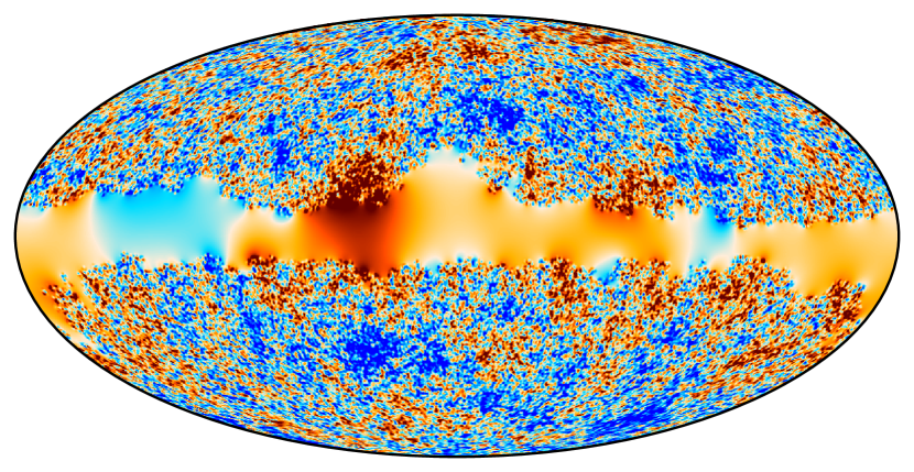
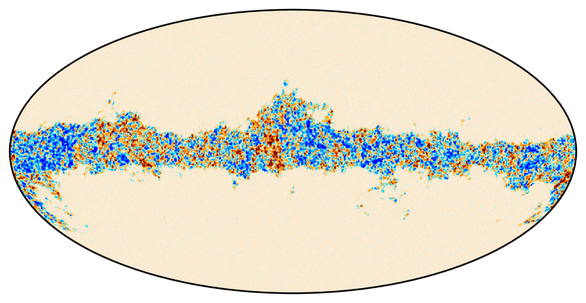
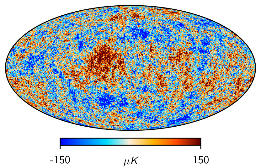
Figure 4: Illustration of the Gibbs sampling procedure. The full sample $\@vec{s}$ (bottom panel) is the sum of the mean field map ${\hat{\@vec{x}}}$ (top panel) and a fluctuation map ${\hat{\@vec{y}}}$ (middle panel).

Within the simple template fitting approach described above, the higher-order CMB fluctuations are treated as a noise term. Since the CMB fluctuations are Gaussian and isotropic, this term does not lead to any bias in the central estimates, but it does increase the variance. An alternative approach is to exploit the assumptions of isotropy and Gaussianity to estimate the CMB signal jointly with the dipole parameters, adopting the following data model,

$$\@vec{d}=\@vec{s}+\@vec{n},$$ (10)

where

$$\@vec{s}=\@vec{s}(\hat{n})=\sum_{\ell,m}a_{\ell m}Y_{\ell m}(\hat{n})$$ (11)

now is an isotropic and Gaussian random field with some angular power spectrum $C_{\ell}$. Note that the previously defined dipole is contained within $\@vec{s}$ in the form of $\@tens{T}\@vec{a}=\sum_{\ell=0}^{1}\sum_{m}a_{\ell m}Y_{\ell m}(\hat{n})$.

To estimate $\@vec{s}$ and $C_{\ell}$ jointly, we employ the Gibbs sampling algorithm described by Eriksen et al. (2004). This algorithm draws samples from the probability density $P(\@vec{s},C_{\ell}|\@vec{d})$. Since it is difficult to sample directly from this joint distribution, we instead employ Gibbs sampling, and perform consecutive sampling from each conditional density, $P(\@vec{s}|C_{\ell},\@vec{d})$ and $P(C_{\ell}|\@vec{s},\@vec{d})$, which according to Gibbs sampling theory will converge to being samples from the joint density $P(\@vec{s},C_{\ell}|\@vec{d})$. Thus, the two Gibbs sampling steps are

$$\@vec{s}^{i+1} \leftarrow P(\@vec{s}|C_{\ell}^{i},\@vec{d}),$$ (12)

$$C_{\ell}^{i+1} \leftarrow P(C_{\ell}|\@vec{s}^{i+1}).$$ (13)

For more information on the sampling process for the CMB power spectrum in Eq. 13, we again refer to Eriksen et al. (2004). However, we note that the inverse-gamma sampler described in that paper is only employed for multipoles $\ell\geq 2$ in the current analysis. For the first two elements, we manually set $C_{\ell}$ to a numerical large value of $10^{12}\thinspace\mu$K², which effectively corresponds to imposing no informative priors on the monopole and dipole moments.

In our context we are mostly interested in the map sampling process in Eq. 12. In effect, the sky sample $\@vec{s}^{i}$ uses phase information in the data $\@vec{d}$ outside the mask to extrapolate into the missing pixels. The result is a constrained realization with the assumed power spectrum $C_{\ell}$, such that the full map is a sample from the desired target distribution.

The map sampling process in Eq. 12 is performed in two steps. First we compute the so-called mean field map by solving the Wiener filter mapmaking equation for $\hat{\@vec{x}}$,

$$\left(\@tens{S}^{-1}+\@tens{Y}^{t}\@tens{N}^{-1}\@tens{Y}\right){\hat{\@vec{x}}}=\@tens{Y}^{t}\@tens{N}^{-1}\@vec{d}.$$ (14)

Here, $\@tens{S}$ is a diagonal prior matrix that contains the assumed power spectrum, $\@tens{Y}$ denotes spherical harmonic transforms, and $\@tens{N}$ is the noise covariance matrix. The equation above is a Wiener filter, and the resulting map ${\hat{\@vec{x}}}$ is as such biased. To unbias the full sample, we have to add a fluctuation term. We obtain the corresponding fluctuation map by solving the following expression for ${\hat{\@vec{y}}}$,

$$\left(\@tens{S}^{-1}+\@tens{Y}^{t}\@tens{N}^{-1}\@tens{Y}\right){\hat{\@vec{y}}}=\@tens{S}^{-1/2}\mathbf{\omega_{1}}+\@tens{Y}^{t}\@tens{N}^{-1/2}\mathbf{\omega_{2}}.$$ (15)

Here, $\mathbf{\omega_{1}}$ and $\mathbf{\omega_{2}}$ are two independent Gaussian white noise maps with zero mean and unit variance. The full sample $\@vec{s}$ is then the sum of ${\hat{\@vec{x}}}$ and ${\hat{\@vec{y}}}$.

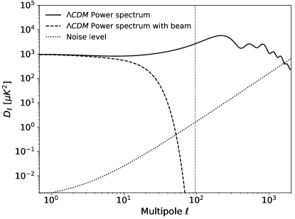
Figure 5: Overview of signal and noise power spectra adopted for the Monte Carlo simulations. The solid line shows the best-fit Planck $\Lambda$CDM power spectrum, and the dashed line shows the same, but convolved with a $6^{\circ}$ FWHM Gaussian beam. The dotted line shows the noise spectrum for white uncorrelated noise with $\sigma_{0}=1\thinspace\mu$K per pixel at a HEALPix resolution of ${N_{\mathrm{side}}}=32$. The vertical dotted line shows the harmonic space truncation limit of $\ell_{\textrm{max}}=95$.

The key advantage of sampling from the full distribution is that one simultaneously takes into account all multipole scales and all elements of the coupling kernel shown in Fig. 2. To illustrate this visually, Fig. 4 shows the different maps involved in the sampling procedure for some typical mask. The top panel shows the Wiener filter component. Note that this map contains small-scale structures in the unmasked regions, but only smooth structures in the masked regions. However, critically, it is not zero inside the mask. On the contrary, because of the assumptions of statistical isotropy and Gaussianity, the field inside the mask must show some degree of phase correlation with the unmasked regions, and this is precisely the information that allows partial reconstruction inside the mask.

Of course, this extrapolation is only supported for large angular scales. The fluctuation term, shown in the middle panel, therefore compensates for the fluctuation power that is lost due to the mask and noise, such that the sum of the two components, shown in the bottom panel, is a single full-sky map that is consistent with the original data. Note, however, that this map contains a significant stochastic component, and a full ensemble of such Gibbs samples is therefore required to adequately describe both the mean and covariance of the true underlying signal.

3 Simulations

We have now established two different methods for estimating dipole parameters from a foreground-cleaned CMB map with partial sky coverage. In order to assess the relative performance of these two methods, we perform Monte Carlo simulations for both algorithms, and compare the resulting uncertainties.

3.1 Monte Carlo procedure

For the standard template fitting approach, the procedure is defined as follows:

1. Generate $N$ simulated CMB skies $d_{[1,...,N]}$ based on a $\Lambda$CDM power spectrum.

2. Apply mask $\@tens{M}$ to each sample.

3. Compute best-fit dipole parameters $A$, $l$ and $b$ for each sample with Eqs. 2–5.

4. Report the standard deviation for each parameter, $\sigma_{A}$, $\sigma_{l}$ and $\sigma_{b}$.

For the Wiener filter approach, the procedure is similar, but additionally involves an intermediate sampling loop for each realization:

1. Generate $N$ simulated CMB skies $d_{[1,...,N]}$ based on a $\Lambda$CDM power spectrum.

2. Apply mask $\@tens{M}$ to each sample.

3. For each masked CMB map:

4. 1. Draw $n$ full-sky Wiener filter samples $s_{[1,...,n]}$.

   2. Compute dipole parameters $A$, $l$ and $b$ for each sample.

   3. Compute single-realization standard deviations $\sigma_{A}^{i}$, $\sigma_{l}^{i}$ and $\sigma_{b}^{i}$.

5. Report the mean of $\sigma_{A}^{i}$, $\sigma_{l}^{i}$ and $\sigma_{b}^{i}$.

The template fitting analysis is implemented using the HEALPix fit_dipole routine (Górski et al. 2005), while the Wiener filter analysis is performed using the Commander code Eriksen et al. (2004).

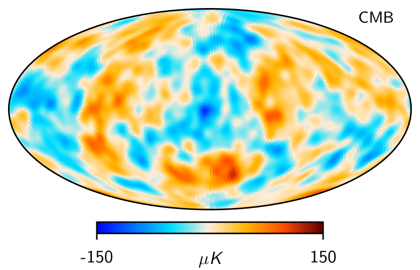
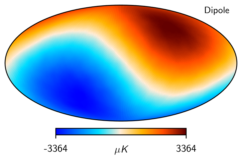
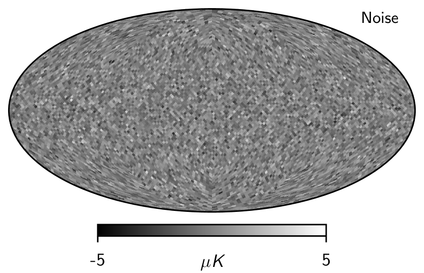
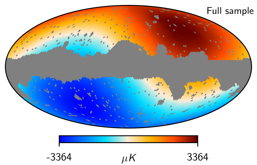
Figure 6: Components used to construct each Monte Carlo realization. These are the higher-order CMB fluctuations (top panel), the CMB dipole (second panel), and instrumental noise (third panel). The bottom panel shows the sum of the three components with a mask super-imposed.

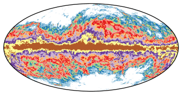
Figure 7: Analysis masks used for the Monte Carlo comparison. The unmasked sky fractions from the smallest to the largest mask are 92 % (brown), 84 % (yellow), 76 % (purple), 68 % (lilac), 60 % (bright orange), 52 % (red), 44 % (bright red), 36 % (green), 28 % (cyan) and 20 % (light blue).

3.2 CMB simulations

For our simulated sky maps, we adopt the same model as in Eqs. 10–11, but this time we explicitly include support for an instrumental beam with Legendre expansion $b_{\ell}$,

$$\@vec{d}=\@vec{s}+\@vec{n}=\sum_{\ell=0}^{\ell_{max}}\sum_{m={-\ell}}^{\ell}b_{\ell}a_{\ell m}Y_{\ell m}+\@vec{n}.$$ (16)

We generate multipoles with $\ell\geq 2$ using Healpy’s synfast routine, drawn from the Planck 2018 best-fit $\Lambda$CDM power spectrum (Planck Collaboration VI 2018). For the dipole component, we adopt $A=3364.0\thinspace\mu$K, $l=264.1^{\circ}$ and $b=48.3^{\circ}$. No monopole is added.

For both the template and Wiener filter approaches, we establish ensembles of 100 realizations. To limit the computational speed involved in the Wiener filter stage, which requires iterative sampling, we choose to perform the analysis at a HEALPix resolution of $N_{\mathrm{side}}=32$, corresponding to a pixel size of about $1.8^{\circ}$. This is sufficient to capture all features that are relevant for dipole estimation.

For high-sensitivity experiments such as Planck, the direct template fitting approach is largely insensitive to specific details of the instrumental noise, as the dominant noise contributor is the CMB fluctuations, and $\@vec{n}$ may be safely disregarded in this framework. However, for the Wiener filter approach some care is warranted also for this term. In particular, the details of $\@vec{n}$ determine how aggressively the estimator is able to extrapolate into the masked region. For the method to be accurate and unbiased, it is important that the data model in Eq. 16 actually is a good representation of the observations in question.

First, since we perform our analysis at $N_{\mathrm{side}}=32$, the highest resolvable multipole moment is given roughly by $\ell_{\textrm{max}}\approx 3N_{\mathrm{side}}=96$. In order to suppress the signal above this $\ell_{\textrm{max}}$, which is not supported by Eq. 16, we smooth the simulated CMB realizations with a $6^{\circ}$ FWHM Gaussian beam with a Legendre expansion given by (Tegmark 1997)

$$b_{\ell}=\exp\left[-\frac{1}{2}\ell(\ell+1)\left(\frac{\text{FWHM}\cdot\pi}{180}\cdot\frac{1}{\sqrt{8\ln 2}}\right)^{2}\right].$$ (17)

Next, to avoid ringing artefacts from the truncation limit around the mask edge, we have to ensure that the effective signal-to-noise ratio is negligible at $\ell_{\textrm{max}}$. We do this by adding regularization noise with a standard deviation of $\sigma_{0}=1\thinspace\thinspace\mu$K per pixel. In harmonic space, this corresponds to a flat noise spectrum with an amplitude given by (Tegmark 1997)

$$N_{\ell}=\sigma_{0}^{2}\cdot\frac{4\pi}{N_{\text{pix}}}\cdot\frac{\ell(\ell+1)}{2\pi}.$$ (18)

Figure 5 summarizes the simulated data in terms of signal and noise power spectra. Note that with these choices of parameters, the effective signal-to-noise ratio at $\ell=95$ is smaller than 0.01. The individual components involved in the simulated map are illustrated in Fig. 6.

Since the elements of the coupling kernel depend on the sky fraction and on the shape of the mask, we repeat the Monte Carlo analysis for a variety of different masks with sky fractions ranging from 20 to 95 %, shown in Fig. 7. These masks were already used for a similar purpose in Planck Collaboration III (2018).

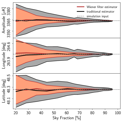
Figure 8: CMB solar dipole parameter uncertainties as a function of sky fraction; The thick red and black lines show the posterior means derived by the Wiener filter method and the traditional method respectively; The shaded bands are the corresponding $\pm 1\sigma$ confidence intervals; The horizontal dashed lines mark the true dipole parameters that were used as input for the simulations

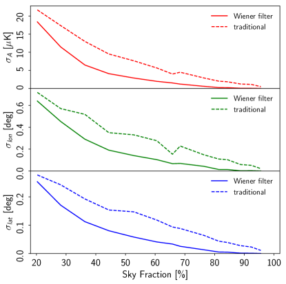
Figure 9: Absolute uncertainties of solar dipole parameters estimated with Wiener filter method (solid lines) and traditional method (dashed lines) as a function of sky fraction

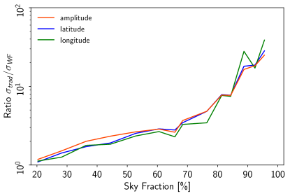
Figure 10: Ratio of uncertainties derived by traditional method and Wiener filter method as a function of sky fraction.

4 Results

We are now ready to present the main result of this paper, which is a quantitative comparison of the template fitting and Wiener filter approaches to dipole parameter estimation. For each mask shown in Fig. 7, we analyse 100 independent Monte Carlo realizations with both methods.

The main result is summarized in Fig. 8, where we show the mean dipole parameters and their corresponding statistical uncertainties as a function of the sky fraction. From top to bottom, the panels show the dipole amplitude, the longitude, and the latitude. The thick red lines show the mean of the derived solar dipole parameters using the Wiener filter technique, and the regions shaded in red show the corresponding $\pm 1\sigma$ confidence intervals. The equivalent results derived using the traditional method are shown in black and gray. We mark the true dipole parameters as horizontal dashed lines.

We find that the uncertainties derived by the Wiener filter technique are significantly reduced compared to the traditional method. This effect is strongest for large sky fractions, for which it is easier to extrapolate into the masked regions. In contrast, for small sky fractions the extrapolation is very unreliable, and the two methods therefore give very similar results.

In some cases in Fig. 8 it may appear as if the traditional method yields smaller uncertainties than the Wiener filter at small sky fractions, especially for the longitude and latitude where the upper confidence interval boundary is in fact below that of the Wiener filter method. However, this is not actually the case, since the grey band is also shifted to lower values due to statistical fluctuations of the derived means. To make this more explicit, we plot the absolute uncertainties of the two methods in Fig. 9, and their ratios in Fig. 10. We see that for large sky fractions (above $\approx 85\%$) the Wiener filter uncertainties are reduced by a factor of 10 or more for all parameters. At a sky fraction of about $50\%$, the uncertainties drop to roughly half of those of the traditional method.

5 Conclusions

Table 1: Comparison of Solar dipole measurements from COBE, WMAP, and Planck.

     Galactic coordinates

     Amplitude      $$l$$      

Experiment      K      [deg]      [deg]      Reference

COBE ^a,b.                        Lineweaver (1997)

WMAP ^c.                        Hinshaw et al. (2009)

LFI 2015 ^b.                        Planck Collaboration II (2016)

HFI 2015 ^d.                        Planck Collaboration VIII (2016)

LFI 2018 ^b.                        Planck Collaboration II (2018)

HFI 2018 ^d.                        Planck Collaboration III (2018)

NPIPE ^a,c.                        Planck Collaboration (2020)

^aStatistical and systematic uncertainty estimates are added in quadrature.

^bComputed with naive dipole estimator that does not account for higher-order CMB fluctuations.

^cComputed with Wiener filter estimator that estimates, and marginalizes over, higher-order CMB fluctuations jointly with the dipole.

^dHigher-order CMB fluctuations are accounted for by subtracting a dipole-adjusted CMB map from frequency maps prior to dipole estimation.

In this paper we have quantitatively compared two numerical techniques for estimating the dipole parameters from a CMB map. The first method is basic template fitting regression with partial sky data, while the second method relies on Wiener filtering. The main difference between the two methods lies in their treatment of partial sky observations. Specifically, masking parts of the sky introduces couplings between small-scale CMB fluctuations and the dipole. The traditional template fitting procedure disregards this coupling effect, and simply treats the CMB fluctuations as a noise term. In contrast, the Wiener filter approach exploits the fact that these fluctuations represent a statistically isotropic and Gaussian random field to partially reconstruct the field inside the mask, and thereby reduce the overall uncertainties.

We apply both methods to an ensemble of 100 Monte Carlo realizations for sky fractions ranging from 20 to 95 %, and derive uncertainties as a function of sky fraction. We find that the Wiener filter approach leads to significantly reduced uncertainties for typical sky fractions used in this type of analyses. For example, at $f_{\textrm{sky}}\approx 60\%$ the uncertainties are reduced by a factor of $\approx 3$, while at $f_{\textrm{sky}}\approx 85\%$ they are reduced by a factor of $\approx 8$.

Table 1 shows a comparison of measurements of the CMB solar dipole made by COBE, WMAP and (various generations of) Planck, and is a direct reproduction of Table 10 from Planck Collaboration (2020). Most of these analyses employed sky fractions around 80 %. For this sky fraction, we see from Fig. 9 that the uncertainty on the amplitude due to small-scale CMB fluctuations is about $2.5\thinspace\mu$K using the template fitting approach. In contrast, the total uncertainty for COBE was 23 $\mu$K, and for WMAP it was 8 $\mu$K. As such, the contribution from CMB confusion was sub-dominant for both these experiments. Nevertheless, it is important to note that WMAP was indeed the first experiment to implement this method for this particular purpose (Hinshaw et al. 2009), even though it may not have been critically important.

For Planck, the situation is fundamentally different. For this experiment, the raw uncertainty from instrumental noise and systematics is smaller than 1 $\mu$K, and the CMB confusion has therefore become a dominant factor. In the LFI processing, this contribution was simply included in the error budget, leading to a final uncertainty of 3 $\mu$K. For HFI, however, a different approach was taken, in that an estimate of the CMB fluctuations was removed from the raw data prior to template fitting. At first sight, this approach appears to eliminate the CMB confusion term entirely, evading the topic discussed in this paper. However, it is important to note that for this approach to be unbiased, the CMB template that is being subtracted must itself have a vanishing dipole moment. Determining the dipole moment of this map is therefore equivalent to the problem described in this paper. For the HFI analyses summarized in Table 1, this determination was performed with a very small mask, which in effect assumes that the component separation method of choice (see Planck Collaboration IV 2018 for details) is able to remove foregrounds accurately even in the central galactic plane.

The last row in Table 1 lists results for the most recent Planck analysis, which is informally referred to as NPIPE. NPIPE represents the first joint analysis of the Planck LFI and HFI data sets, using a common machinery to reduce the raw time-ordered data into final sky maps. One important difference between these maps and earlier versions of the Planck data is that the NPIPE maps retain the solar dipole for both LFI and HFI. It is therefore, for the first time, possible to compute a single coherent all-Planck dipole with these sky maps. The results from this analysis are presented in Sect. 8 of Planck Collaboration (2020), and employ the Wiener filter methodology described in this paper. The values reported in Table 1 correspond to a sky fraction of 81 %, which represents a compromise between maximizing available data and minimizing foreground-induced systematic effects. We believe that the values reported for NPIPE in Table 1 represent the most conservative and statistically robust estimate of the CMB solar dipole published to date.