Anisotropic Kondo screening induced by spin-orbit coupling in quantum wires

Abstract

Using the numerical renormalization group (NRG) method we study a magnetic impurity coupled to a quantum wire with Rashba and Dresselhaus spin-orbit coupling (SOC) in an external magnetic field. We consider the low-filling regime with the Fermi energy close to the bottom of the band and report the results for local static and dynamic properties in the Kondo regime. In the absence of the field, local impurity properties remain isotropic in spin space despite the SOC-induced magnetic anisotropy of the conduction band. In the presence of the field, clear fingerprints of anisotropy are revealed through the strong field-direction dependence of the impurity spin polarization and spectra, in particular of the Kondo peak height. The detailed behavior depends on the relative magnitudes of the impurity and band $g$-factors. For the case of impurity $g$-factor somewhat lower than the band $g$-factor, the maximal Kondo peak supression is found for field oriented along the effective SOC field axis, while for a field perpendicular to this direction we observe a compensation effect (“revival of the Kondo peak”): the SOC counteracts the Kondo peak splitting effects of the local Zeeman field. We demonstrate that the SOC-induced anisotropy, measurable by tunneling spectroscopy techniques, can help to determine the ratio of Rashba and Dresselhaus SOC strengths in the wire.

I Introduction

The emergence of spin-orbit coupling as a major design principle in the development of new information technologies Žutić et al. (2004); Bader and Parkin (2010), especially after the discovery of topological insulators Hasan and Kane (2010), has intensified studies of systems where SOC is determinant in providing access to the spin degree of freedom Winkler (2003); Manchon et al. (2015). One of the main objectives is to incorporate spintronic ideas into contemporary technologies, which are overwhelmingly reliant on semiconducting materials Fabian et al. (2007). In this new paradigm, one aims spin injection, manipulation and detection using semiconductor structures similar to those already in widespread use in standard semiconductor electronics. Electron correlations and SOC may combine to produce new emergent behavior Pesin and Balents (2010); Witczak-Krempa et al. (2014); Rau et al. (2016); Schaffer et al. (2016), as e.g. in iridates, $\rm{Sr_{2}IrO_{4}}$ Kim et al. (2008). The sensitivity of the Kondo effect Bulla et al. (2008); Hewson (1993), the quintessential many-body phenomenon, to magnetic anisotropy Romeike et al. (2006a, b); Roosen et al. (2008); Otte et al. (2008); Žitko et al. (2008, 2009); Pletyukhov et al. (2010); Žitko and Pruschke (2010); Misiorny et al. (2011a, b); Žitko et al. (2011); Höck and Schnack (2013); Blesio et al. (2019) provides opportunities for novel devices. In this work, the authors use the numerical renormalization group (NRG) method Bulla et al. (2008) to study in unbiased manner an impurity in the Kondo regime under the combined effect of SOC Meir and Wingreen (1994); Malecki (2007); Žitko and Bonča (2011); Zarea et al. (2012); Mastrogiuseppe et al. (2014); Wong et al. (2016); Chen et al. (2016); de Sousa et al. (2016); Chen and Han (2017) and external magnetic field. More specifically, we consider a magnetic impurity in contact with a one-dimensional (1D) quantum wire, which is subjected to Rashba Bychkov and Rashba (1984) and Dresselhaus Dresselhaus (1955) SOC, with the Fermi energy placed close to the bottom of the band, which is the regime relevant for some of the proposed applications Kitaev (2001); Oreg et al. (2010); Lutchyn et al. (2010); Nadj-Perge et al. (2014); Lutchyn et al. (2018); Saldaña et al. (2019).

The main result is sketched in Fig. 1. The wire is oriented along the $x$-axis and, for simplicity, pure Rashba SOC is considered here, hence the effective SOC magnetic field $\mathbf{B}_{\rm SO}$ (antiparallel green arrows) points along the $y$-axis. An external magnetic field acts on both the impurity and the wire with different $g$ factors, denoted as $g_{\mathrm{imp}}$ and $g_{w}$, respectively. In order to probe the physical origins of the various contributions to the impurity total spin polarization, we consider two cases, viz., one with $g_{\mathrm{imp}}=0$ and another with $g_{\mathrm{imp}}\neq 0$. We consider the case of $T\ll T_{K}$, where $T_{K}$ is the Kondo temperature for finite-SOC and vanishing external magnetic field $\mathbf{B}$. If $\mathbf{B}$ points along the $y$-axis (red arrow), the Kondo peak is suppressed (red sketch). However, for $\mathbf{B}$ along the $x$ or $z$-axis (blue arrow), the Kondo peak persists (blue sketch). The impurity spin polarization is also anisotropic: for $\mathbf{B}$ along $y$-axis, the impurity is only slightly polarized in the direction of $\mathbf{B}$ (horizontal red arrow), while for $\mathbf{B}$ along $x$ or $z$ axis the impurity is considerably more polarized, but the spin polarization is oriented opposite to $\mathbf{B}$ (vertical blue arrow). One might be led to expect that the stronger suppression of the Kondo peak for $\mathbf{B}$ applied along the $y$-axis implies stronger polarization of the quantum wire when the external magnetic field is applied along this direction. However, this is not the case: the inset to Fig. 1 shows that in the presence of SOC the wire spin polarization, $\langle S_{i}^{\rm w}\rangle$ not (a), is always reduced compared to the zero-SOC case, but the supression is actually greater for the case of external field along the effective SOC-field direction. The stronger suppression of the Kondo peak for $\mathbf{B}$ along the $y$-axis hence cannot be explained by the polarization of the conduction electrons and one instead needs to consider dynamic effects, as we do in the following.

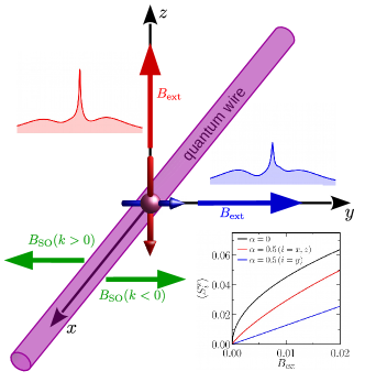
Figure 1: Sketch of the main results. The impurity (purple sphere) is coupled to the quantum wire (purple line). The antiparallel effective $\mathbf{B}_{\rm SO}$ magnetic field (green arrows) acts along the $y$-direction. The situation depicted is that for $g_{\rm imp}=0.4g_{\rm w}$, with the impurity more weakly coupled to the external magnetic field $\mathbf{B}$ than the quantum wire. When $\mathbf{B}$ is applied along the $y$-axis (large blue arrow), the Kondo peak is suppressed and split (blue curve),with the impurity polarized parallel to $\mathbf{B}$ (small blue arrow). When $\mathbf{B}$ is applied along the $z$-axis (red arrow), the Kondo peak is more robust (red curve), yet the impurity polarization is stronger (small red arrow) and furthermore it points in a direction opposite to $\mathbf{B}$. Inset: spin polarization of the wire, $\langle S_{i}^{\rm w}\rangle$, as a function of $\mathbf{B}$ applied along the different axes. The black curve corresponds to zero SOC, $\alpha=0$.

II Model and Hybridization Function

II.1 Model

The wire Hamiltonian is

$$H_{\mathrm{wire}} =\sum_{k}\Psi^{\dagger}_{k}{\cal H}_{\mathrm{wire}}\Psi_{k},$$ (1)

$${\cal H}_{\mathrm{wire}} =\left(\varepsilon_{k}-\mu\right)\sigma_{0}+\mathbf{B}_{\rm tot}\!\cdot{\bm{\sigma}}.$$ (2)

Here $\Psi^{\dagger}_{k}=(c^{\dagger}_{k\uparrow},c^{\dagger}_{k\downarrow})$, $c^{\dagger}_{k\sigma}$ creates an electron with wave vector $k$ and spin $\sigma=\uparrow,\downarrow$, $\varepsilon_{k}=-2t\cos k$ is the tight-binding dispersion relation where $t$ is the nearest-neighbor hopping matrix element, $\mu$ is the chemical potential, $\mathbf{B}_{\rm tot}\!=g_{\rm w}\mathbf{B}+\mathbf{B}_{\rm SO}$​ represents the combined effect of an external magnetic field $\mathbf{B}=(B_{x},B_{y},B_{z})$ and an effective $k$-dependent spin-orbit magnetic field Manchon et al. (2015) ${\bf B}_{\rm SO}(k)=\sin k(\beta,-\alpha,0)$, where the couplings $\alpha$ and $\beta$ (measured in energy units) are the Rashba Bychkov and Rashba (1984) and Dresselhaus Dresselhaus (1955) SOC strengths, respectively. The vector of Pauli matrices ${\bm{\sigma}}=\{\sigma_{x},\sigma_{y},\sigma_{z}\}$ and the identity matrix $\sigma_{0}$ act on spin space. For simplicity, we set the Bohr magneton to $\mu_{B}=1$, and the factor $\nicefrac{{1}}{{2}}$ from ${\bm{S}}=\nicefrac{{\bm{\sigma}}}{{2}}$ has been absorbed into $g_{\rm w}$. We parameterize both SOCs as $\theta_{\rm SO}=-\tan^{-1}\nicefrac{{\alpha}}{{\beta}}$, such that $\beta=\gamma\cos\theta_{\rm SO}$ and $-\alpha=\gamma\sin\theta_{\rm SO}$, i.e. $\theta_{\rm SO}$ is the angle between the effective magnetic field ${\bf B}_{\rm SO}(k)$ (for positive $k$) and the $x$-axis. For pure Rashba SOC with $\beta=0$ ($\theta_{\rm SO}=\pm\nicefrac{{\pi}}{{2}}$), the effective field points along the $y$-axis (see Fig. 1), while for pure Dresselhaus SOC with $\alpha=0$ ($\theta_{\rm SO}=0,\pi$), it points along the $x$-axis.

To study the Kondo state in this system, the quantum wire is coupled to an Anderson impurity, which is modeled as

$$H_{\rm imp}=\sum_{s}\varepsilon_{d}n_{\sigma}+Un_{\uparrow}n_{\downarrow}+g_{\rm imp}\mathbf{B}\cdot{\bm{S}},$$ (3)

where $d^{\dagger}_{\sigma}$ ($d_{\sigma}$) creates (annihilates) an electron with orbital energy $\varepsilon_{d}$ and spin $\sigma=\uparrow,\downarrow$, $n_{\sigma}=d^{\dagger}_{\sigma}d_{\sigma}$, and $U$ represents Coulomb repulsion. The third term accounts for the Zeeman interaction of the impurity’s magnetic moment $g_{\rm imp}{\bm{S}}$. The hybridization between the impurity and the conduction electrons is given by

$$H_{\mathrm{hyb}}=\sum_{k\sigma}\left(V_{k}d^{+}_{\sigma}c_{k\sigma}+{\rm H.c.}\right).$$ (4)

In this work we consider the case of $V_{k}\equiv V$. The Fermi energy is close to the bottom of the band, $\mu=-1.0$, and we use the $\gamma=0$ half-bandwidth $D=2t=1.0$ as the energy unit. Unless stated otherwise, we use $U=0.5$, $\epsilon_{d}=-U/2$, $V=0.07$, and $g_{\rm w}/g_{\rm imp}=2.5$ not (b) (with $g_{\rm w}=1$ and $g_{\rm imp}=0.4$), $|\mathbf{B}|=0.01$. We take $\gamma=\sqrt{\alpha^{2}+\beta^{2}}=0.5$ as being fixed and perform most calculations for $\theta_{\rm SO}=\nicefrac{{-\pi}}{{2}}$ (i.e., Rashba-only). The Kondo temperature of this system is $T_{K}\approx 1.16\times 10^{-2}$​.

The single-electron bands described by H are shown in Fig. 2: panel a for zero $\mathbf{B}$, and panels b,c,d for $|\mathbf{B}|=0.01$ oriented along $x$, $y$, and $z$-axis. For $\theta_{\rm SO}=\nicefrac{{-\pi}}{{2}}$, ${\bf B}_{\rm SO}(k)$ is oriented along the $y$-axis, thus the bands for $\mathbf{B}$ along the $x$ and $z$-axis are identical, but they differ from those for $\mathbf{B}$ along the $y$-axis, reflecting the anisotropy introduced by SOC. The dependence of the direction of $\mathbf{B}_{\rm SO}$ on the sign of $k$ can be read from the difference in the splitting of the bands in panel c: for $k>0$ $\mathbf{B}_{\rm SO}$ opposes $\mathbf{B}$, generating a smaller band splitting, while for $k<0$ $\mathbf{B}_{\rm SO}$ aligns with $\mathbf{B}$, increasing the band splitting. In the other cases the bands have even parity.

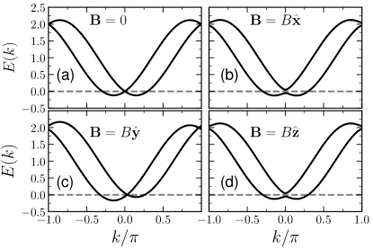
Figure 2: Band structure of a quantum wire for $\gamma=0.5$, $\theta_{\rm SO}=\nicefrac{{-\pi}}{{2}}$ (Rashba SOC) and different values of external field (a) $B=0$, (b) $\mathbf{B}=B\hat{\mathbf{x}}$, (c) $\mathbf{B}=B\hat{\mathbf{y}}$, (d) $\mathbf{B}=B\hat{\mathbf{z}}$, with $B=0.01$.

II.2 Hybridization function

The impurity Green’s function $\hat{G}_{\rm imp}(\omega)$ can be written as

$$\hat{G}_{\rm imp}(\omega)=\left[\left(\omega-\varepsilon_{d}\right)\sigma_{0}-\hat{\Sigma}^{\rm(int)}(\omega)-\hat{\Sigma}^{(0)}(\omega)\right]^{-1},$$ (5)

where $\hat{\Sigma}^{\rm(int)}(\omega)$ is the interaction self-energy, while $\hat{\Sigma}^{(0)}(\omega)=\sum_{k}\hat{V}\hat{G}_{\mathrm{wire}}(k,\omega)\hat{V}^{\dagger}$ is the hybridisation self-energy, with $\hat{V}=V_{0}\sigma_{0}$ and $\hat{G}_{\mathrm{wire}}(k,\omega)=\left[\omega\sigma_{0}-{\cal H}_{\mathrm{wire}}\right]^{-1}$. One finds

$$\begin{split}\hat{\Sigma}^{(0)}(\omega)=\sum_{k}F(k,\omega)\Bigl{[}\left(\cos k+\mu+\omega\right)\sigma_{0}+\\ (\alpha\sigma_{y}-\beta\sigma_{x})\sin k-g_{\rm w}\mathbf{B}\cdot{\bm{\sigma}}\Bigr{]},\end{split}$$

where

$$F(k,\omega)=\frac{-V^{2}}{2\left(\alpha B_{y}-\beta B_{x}\right)\sin k+B^{2}+\gamma^{2}\sin^{2}k-(\cos k+\mu+\omega)^{2}}.$$

For a magnetic field applied along an arbitrary direction, $\hat{\Sigma}^{(0)}(k,\omega)$ has finite off-diagonal terms and we have to deal with a spin-mixing hybridization function Liu et al. (2016); Osolin and Žitko (2017)

$$\hat{\Gamma}(\omega)=\frac{1}{2i}\int_{-\pi}^{\pi}\left[\hat{\Sigma}^{(0)}(k,\omega-i0^{-})-\hat{\Sigma}^{(0)}(k,\omega+i0^{+})\right]dk.$$ (6)

This positive-definite Hermitian matrix can be decomposed in terms of Pauli matrices as $\hat{\Gamma}(\omega)=\sum_{i\in\{0,x,y,z\}}d_{i}(\omega)\sigma_{i}$, where all $d_{i}(\omega)$ are real quantities. In particular, $d_{0}(\omega)$ is proportional to the conduction-band density of states not (c).

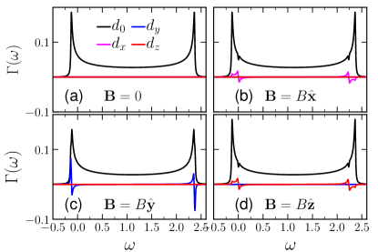
Figure 3: Hybridization function coefficients $d_{i}(\omega)$ for (a) zero field, and for (b,c,d) field oriented along the different axes.

In the absence of SOC, for $B=0$, only $d_{0}(\omega)$ is non-zero, while for $B>0$, the coefficient $d_{i}$ in the field direction is also finite, with a value that does not depend on the field direction, thus manifesting the spin isotropy. In the presence of SOC, the rotation invariance is broken, see Fig. 3. For $B=0$ (panel a) again only $d_{0}(\omega)$ is non-zero. For $\mathbf{B}=B\hat{\mathbf{x}}$ (panel b), $d_{0}(\omega)$ exhibits a small dip associated to the lifting of degeneracies at $k=0$ and $\pi$ [see Fig. 2(b)], $d_{x}(\omega)$ is finite, while $d_{y}(\omega)$ and $d_{z}(\omega)$ remain zero. The results in panel d, for the field along $z$-axis, are equivalent up to a permutation of the $x$ and $z$ axes. For $\mathbf{B}=B\hat{\mathbf{y}}$ (panel c), $d_{0}(\omega)$ is different from the corresponding curve in panels b and d, and $d_{y}(\omega)$ is different from $d_{x}(\omega)$ and $d_{z}(\omega)$ in those panels. This clearly shows how the $y$-axis becomes distinct, since the Rashba SOC tends to align the spins of the conduction electrons along this axis. The anisotropy of $\hat{\Sigma}^{(0)}$ affects the screening of impurity local moment Bulla et al. (2008), thus the SOC in the wire is experimentally detectable by probing the properties of the Kondo state. The problem bears some similarity with the problem of a quantum dot with ferromagnetic leads Sindel et al. (2007); Choi et al. (2004); Martinek et al. (2005, 2003a, 2003b); Žitko et al. (2012), but the focus here is on SOC anisotropy and the ensuing detailed form of the hybridisation function, with complex (and direction-dependent) behavior close to the band edges.

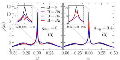
Figure 4: Local density of states $\rho(\omega)$. (a) $g_{\rm imp}=0$ and (b) $g_{\rm imp}=0.4$. Insets: close-ups on the Kondo peak.

III Results

III.1 Impurity Local Density of States

The total impurity LDOS $\rho(\omega)=-\frac{1}{\pi}{\rm Im\,}\mathrm{Tr}\,\hat{G}_{{\rm imp}}(\omega)$ is shown in Fig. 4 for zero field and for fields along the three axis. Two different g-factor values are used: $g_{\rm imp}=0$ (panel a) and $g_{\rm imp}=0.4$ (panel b). The Kondo peak is similarly suppressed for $\mathbf{B}\parallel\hat{\bf y}$ for both g-factor values, slightly more so for finite $g_{\rm imp}$ (see insets), while for $\mathbf{B}\parallel\hat{\bf x}$ or $\hat{\bf z}$ there is a noticeable quantitative difference: the splitting and suppression is much more prominent for vanishing $g_{\rm imp}$. Thus, the picture that emerges is the following: for $g_{\rm imp}=0$ the band polarization results in the inset to Fig. 1 explain the Kondo suppression for any direction of the external magnetic field. However, when the impurity Zeeman effect is turned on, the Kondo suppression for $\mathbf{B}\parallel\hat{\bf y}$ is largely unaffected, while for $\mathbf{B}\parallel\hat{\bf x}$ or $\hat{\bf z}$ it is partially erased, as if the band polarization and the impurity Zeeman effect were canceling each other. In other words, for $\mathbf{B}\parallel\hat{\bf x}$ or $\hat{\bf z}$, a finite Zeeman term at the impurity ($g_{\rm imp}=0.4$, panel b) seems to partially compensate the broad splitting caused by the band polarization (panel a), as it increases the LDOS spectral weight around $\omega=0$, partially reconstructing the Kondo peak.

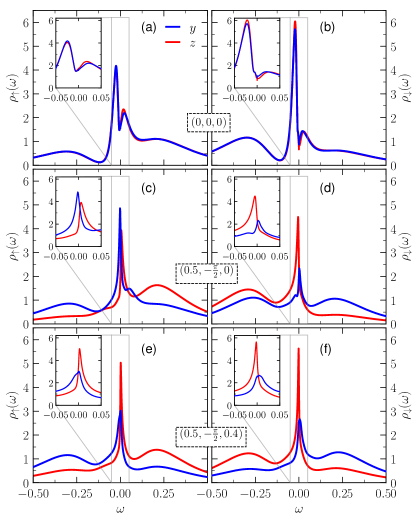
Figure 5: Spectral function resolved along the axis of the applied magnetic field, $\rho_{\sigma_{i}}(\omega)$, with $i\in\{x,y,z\}$; left and right panels correspond to the two projections. Top-row: zero SOC and $g_{\rm imp}=0$ (reference results). Middle-row: Rashba SOC [$\gamma=0.5$, $\theta_{\rm SO}=\nicefrac{{-\pi}}{{2}}$] and $g_{\rm imp}=0$. Bottom-row: Rashba SOC and $g_{\rm imp}=0.4$. In all panels $g_{\rm w}=1.0$, i.e., the quantum wire is spin polarized. The insets show a close-up of the vicinity of the Fermi energy. The tuples straddling both panels for each row indicate the respective values of $[\gamma,\theta_{\rm SO},g_{\rm imp}]$.

III.2 Spin-resolved Local Density of States.

We now reexamine the spectra by resolving them along the magnetization axis defined by the applied external magnetic field, see Fig. 5. The three rows of panels show the results as couplings are gradually turned on: (i) $\gamma=0$, $g_{\rm imp}=0$, (ii) $\gamma=0.5$, $g_{\rm imp}=0$, (iii) $\gamma=0.5$, $g_{\rm imp}=0.4$. For all rows $g_{\rm w}=1.0$. At zero SOC (first row), the results do not depend on the field direction. Since $g_{\rm imp}=0$, the suppression of the Kondo peak and the partial polarization of the impurity is induced by the band polarization alone. In the presence of SOC (second row), $\mathbf{B}\parallel\hat{\bf y}$ differs from $\mathbf{B}\parallel\hat{\bf x}$ or $\hat{\bf z}$. In addition, since the introduction of SOC moves the van-Hove singularity at the bottom of the band to lower energies, away from the Fermi energy, the Kondo peak becomes less asymmetric compared to the $\gamma=0$ results in the first row. Resolving the spectra along the external field direction allows us to see that the Kondo effect is affected more strongly when $\mathbf{B}\parallel\hat{\bf y}$, since, as is more clearly seen in the insets, the Kondo peak polarization is parallel to the applied field for $\mathbf{B}\parallel\hat{\bf y}$ and antiparallel for $\mathbf{B}\parallel\hat{\bf x}$ or $\hat{\bf z}$. The inclusion of a finite $g_{\rm imp}$ (third row) changes this picture only quantitatively, with the impurity becoming less antiferromagnetically correlated with the polarized band for $\mathbf{B}\parallel\hat{\bf x}$ and $\hat{\bf z}$, and becoming more ferromagnetically correlated with the band for $\mathbf{B}\parallel\hat{\bf y}$. This picture is reinforced by calculating the impurity polarization as a function of temperature, see Fig. 6, where one can see that, at low temperature, for $\mathbf{B}\parallel\hat{\bf y}$ and $g_{\rm imp}=0$ (open symbols in panel c), the impurity is barely correlated with the band, becoming ferromagneticaly correlated with it for $g_{\rm imp}=0.4$ (solid symbols). On the other hand, for $\mathbf{B}\parallel\hat{\bf x}$ and $\hat{\bf z}$, (panels b and d), there is a clear Kondo correlation of the impurity with the band for $g_{\rm imp}=0$ (open symbols), which is somewhat weakened by the impurity Zeeman term ($g_{\rm imp}=0.4$, solid symbols). Jointly, these results establish the revival alluded to in Fig. 1, as moving the external field from $\hat{\bf y}$ to $\hat{\bf x}/\hat{\bf z}$ strengthens the Kondo effect (see Fig 9 too).

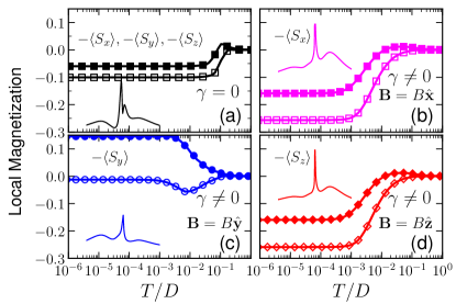
Figure 6: Impurity spin polarization $\langle S_{i}\rangle$ vs temperature. Same parameters as in Figs. 3 and 4, except for panel a, where $\gamma=0$. In panels a to d, open and solid symbols correspond to $g_{\rm imp}=0$ and $g_{\rm imp}=0.4$, respectively. Note that in panel a, since $\gamma=0$, $\langle S_{i}\rangle$ is the same for all $i$ axes, thus only the $x$-axis result is shown. In panels b, c, and d, $i=x$, $y$, and $z$, respectively. Note that the impurity polarization, for directions perpendicular to the applied external field [like, for example, $\langle S_{y}\rangle$ and $\langle S_{z}\rangle$, for $\mathbf{B}\parallel\hat{\bf x}$, panel b], vanish identically, and therefore are not shown. In each panel, a sketch of the impurity’s LDOS, corresponding to $g_{\rm imp}=0$, is shown.

III.3 Temperature dependence of the impurity spin polarization

Now, we track the impurity spin polarization, $\langle S_{i}\rangle$ not (d), as the temperature is reduced from $T=D$ to $\approx 0$, see Fig. 6. By following how the spin components evolve through the three SIAM fixed points, we gain some intuition on how the SOC affects the Kondo state properties. In addition, by comparing the results for $g_{\rm imp}=0$ (open symbols) and $g_{\rm imp}=0.4$ (solid symbols), we discern which effects arise from the band polarization alone, and which are the consequence of the local Zeeman field. An external magnetic field $|\mathbf{B}|=0.01$ is applied along the same $i$-axis along which the impurity spin magnetization -$\langle S_{i}\rangle$ is measured. The results in panel a, without SOC ($\gamma=0$), are the same for all three directions (thus, only the $x$-axis result is shown). The temperature variation of the impurity magnetization reveals the cross-overs between the three SIAM fixed points: free orbital (FO) $\rightarrow$ local moment (LM) $\rightarrow$ strong coupling (SC). At the FO fixed point ($T\lesssim D$), the spin magnetization is negligible for both values of $g_{\rm imp}$ because of the strong charge fluctuations. At the LM fixed point, the local spin starts to form for $T\lesssim U=0.5$ and the open and solid symbols curves start to separate: for $g_{\rm imp}=0$ the impurity polarizes in response to the band polarization and its spin antialigns with the band polarization due to antiferromagnetic Kondo exchange coupling (thus $-\langle S_{i}\rangle<0$), while for $g_{\rm imp}=0.4$ the impurity Zeeman term will counteract this effect (thus $-\langle S_{i}\rangle\gtrsim 0$). As the temperature decreases further ($T\approx U/5=0.1$), the charge fluctuations die down and, for $g_{\rm imp}=0.4$, $-\langle S_{i}\rangle$ reaches a maximum at the LM fixed point and decreases toward the SC fixed point. Because the Zeeman effect is too small to suppress Kondo, the magnetization settles into an $-\langle S_{i}\rangle<0$ plateau located above that for $g_{\rm imp}=0$.

The results for finite SOC are shown in panels b to d. For $\mathbf{B}\parallel\hat{\bf y}$ (panel c), by comparison to the results just described for zero-SOC ($\gamma=0$), we see that the combination of SOC and $\mathbf{B}\parallel\mathbf{B}_{\rm SO}$ considerably weakens the Kondo state resulting from finite $\mathbf{B}$ and $\gamma=0$ (panel a), since the $-\langle S_{i}\rangle\approx 0$ plateau for $g_{\rm imp}=0$ indicates that the impurity is barely correlated to the band, and $-\langle S_{i}\rangle>0$ for $g_{\rm imp}=0.4$. On the other hand, for $\mathbf{B}\parallel\hat{\bf x}$ or $\hat{\bf z}$ (panels b and d), where $\mathbf{B}\perp\mathbf{B}_{\rm SOC}$, the situation is quite different, as it is clear that the Kondo state was strengthened in relation to both the zero-SOC case (panel a) and the finite SOC with $\mathbf{B}\parallel\hat{\bf y}$ case (panel c), illustrating the Kondo ‘revival’ shown in Fig. 9.

III.4 Field dependence of impurity magnetization and Kondo splitting

In Fig. 7, we present how the $g_{\rm imp}=0.4$ impurity magnetization $-\langle S_{i}\rangle$, for $i=x,y,z$, varies with external field intensity ($0\leq B\leq 0.01$), for the field applied along the $i$-axis. The results for $\mathbf{B}\parallel\hat{\bf y}$ (blue curve) and $\mathbf{B}\parallel\hat{\bf x}$ and $\hat{\vec{z}}$ (red curve) evolve smoothly with field intensity, with the $\mathbf{B}\parallel\hat{\bf y}$ curve seemingly having plateaued around $B=0.01$. Thus, the $B=0.01$ results presented in the previous sections may be considered as representative, i.e., there is nothing special about the $B=0.01$ value. In Fig. 8, we show the spin-down projected Kondo peak position, denoted as $\omega_{\downarrow}^{\rm max}$, as a function of $\mathbf{B}$ ($0\leq B\leq 0.01$), for $g_{\rm imp}=0.4$. As for the case of the impurity magnetization, Fig. 7, both curves evolve smoothly with external field, showing again that the $B=0.01$ value is representative of the physical phenomena discussed above.

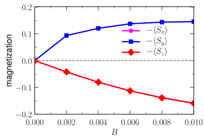
Figure 7: Impurity spin magnetization $-\langle S_{i}\rangle$ vs $|\mathbf{B}|$ for field along different directions, for $g_{\rm imp}=0.4$.

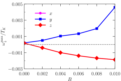
Figure 8: Spin-down projected Kondo peak position $\omega_{\downarrow}^{\rm max}$ as a function of $\mathbf{B}$, for $g_{\mathrm{imp}}=0.4$. The impurity spin polarizes (magnetizes) along (opposite to) the external field for $\mathbf{B}\parallel\hat{\bf y}$, while the reverse occurs for $\mathbf{B}\parallel\hat{\bf x}$ or $\hat{z}$. In other words, the impurity spin correlates antiferromagnetically with the band spins in the latter case, and ferromagnetically for the former case. This is in accordance with the result sketched in Fig. 1.

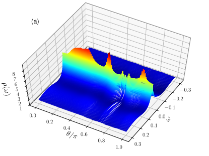
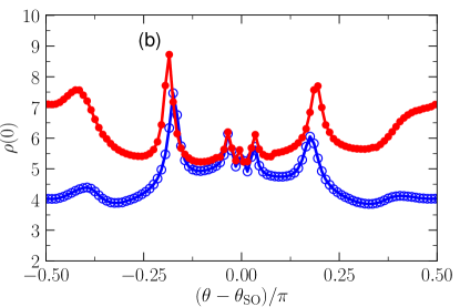
Figure 9: (a) Local density of states $\rho(\omega)$ vs $\omega$ and $\theta$, for $\alpha=0.4$ and $\beta=0.3$ ($\theta_{\rm SO}\approx-0.295\pi$). (b) $\rho(\omega=0)$ vs $\theta-\theta_{\rm SO}$ for $g_{\rm imp}=0$ (blue open symbols) and $g_{\rm imp}=0.4$ (red solid symbols), where $-\nicefrac{{\pi}}{{2}}\leq\theta-\theta_{\rm SO}\leq\nicefrac{{\pi}}{{2}}$ determines the orientation of the external magnetic field in the $xy$ plane in relation to $\theta_{\rm SO}$. Note that the curves have a $\pi$ periodicity. $g_{\rm w}=1$ for both panels.

III.5 Combined effect of Rashba and Dresselhaus SOC

We now consider the generic case with both Rashba and Dresselhaus SOC. Based on what has been shown so far we anticipate that an analysis of the Kondo peak height as a function of the field direction provides information about the direction of $\mathbf{B}_{\rm SOC}$. Since $\theta_{\rm SOC}$ is associated with the ratio $\nicefrac{{\alpha}}{{\beta}}$, its precise determination (e.g. using scanning tunneling spectroscopy) in conjuction with additional measurements Meier et al. (2007); Ho Park et al. (2013); Knox et al. (2018) would give access to the absolute values of $\alpha$ and $\beta$. Panel (a) in Fig. 9 shows a 3D plot of the impurity’s LDOS for the magnetic field in the $xy$ plane as a function of the polar angle $\theta$ between the $x$-axis and the field direction. One can clearly see that the Kondo peak (at $\omega=0$) suffers strong variations as a function of $\theta$. This can be observed in more detail in Fig. 9(b), which shows the impurity LDOS at the Fermi energy (i.e., Kondo peak height) as a function of $\theta-\theta_{\rm SO}$, the direction of the external magnetic field in relation to $\theta_{\rm SO}$, from $-\nicefrac{{\pi}}{{2}}$ to $\nicefrac{{\pi}}{{2}}$. Open (blue) symbols are for $g_{\rm imp}=0$, while solid (red) symbols are for $g_{\rm imp}=0.4$. We note that the spin symmetry of the Hamiltonian requires that the curves in panel (b) should be symmetric around $\theta=\theta_{\rm SO}$. The somewhat delicate NRG numerics at $\omega=0$ is responsible for the observed lack of perfect symmetry. Two broad $\rho(0)$ maxima occur orthogonally to $\theta_{\rm SOC}=-\tan^{-1}\nicefrac{{\alpha}}{{\beta}}$. This is in agreement with the results described above as a ‘revival of the Kondo peak’ for $\mathbf{B}\perp\mathbf{B}_{\rm SOC}$. The presence of other features in the curves indicates that a better strategy to find $\theta_{\rm SO}$ is by exploiting the expected symmetry around $\theta_{\rm SO}$. In any case, this method of finding the Rashba and Dresselhaus couplings can be used as a complementary technique to other proposed procedures Meier et al. (2007); Ho Park et al. (2013); Knox et al. (2018).

A very interesting recent experimental result Bommer et al. (2019) has shown a similar magnetic-field-revealed anisotropy in an InSb quantum wire proximity coupled to a superconductor. In that case, it is the superconducting gap that undergoes a ‘revival’ when the magnetic field is rotated away from the SOC-induced effective magnetic field.

IV Summary and Conclusions

We have shown that Rashba and Dresselhaus SOC in a quantum wire can be investigated through their combined effect on the Kondo ground state of a quantum impurity coupled to the wire. Although SOC breaks the spin isotropy through the introduction of an effective magnetic field $\mathbf{B}_{\rm SO}$, this anisotropy is only manifested when an external magnetic field $\mathbf{B}$ is applied. In that case, the Kondo state properties, like the height of the Kondo peak as well as its Zeeman splitting, are strongly dependent on the relative orientation of $\mathbf{B}_{\rm SO}$ and $\mathbf{B}$. The maximum suppression of the Kondo peak occurs for $\mathbf{B}_{\rm SO}\parallel\mathbf{B}$. Since the orientation of $\mathbf{B}_{\rm SO}$ is given by $\theta_{\rm SO}=\tan^{-1}\nicefrac{{\alpha}}{{\beta}}$, where $\alpha$ and $\beta$ parametrize the Rashba and Dresselhaus interaction, determination of $\theta_{\rm SO}$ can be used to estimate $\nicefrac{{\alpha}}{{\beta}}$. Finally, it would be interesting, as a possible follow-up work, to study the role of the ratio $\nicefrac{{g_{\mathrm{imp}}}}{{g_{w}}}$ more systematically.

V Acknowledgments

GBM acknowledges financial support from the Brazilian agency Conselho Nacional de Desenvolvimento Científico e Tecnológico (CNPq), processes 424711/2018-4 and 305150/2017-0. R. Ž. is supported by Slovenian Research Agency (ARRS) under Program P1-0044.

References

- Žutić et al. (2004) I. Žutić, J. Fabian, and S. Das Sarma, Rev. Mod. Phys. 76, 323 (2004).
- Bader and Parkin (2010) S. Bader and S. Parkin, Annu. Rev. Condens. Matter Phys. 1, 71 (2010).
- Hasan and Kane (2010) M. Z. Hasan and C. L. Kane, Rev. Mod. Phys. 82, 3045 (2010).
- Winkler (2003) R. Winkler, Spin-orbit coupling effects in two-dimensional electron and hole systems, Springer tracts in modern physics (Springer, Berlin, 2003).
- Manchon et al. (2015) A. Manchon, H. C. Koo, J. Nitta, S. Frolov, and R. Duine, Nat. Mater. 14, 871 (2015).
- Fabian et al. (2007) J. Fabian, A. Matos-Abiague, C. Ertler, P. Stano, and I. Zutic, Acta Phys. Slovaca 57, 565 (2007).
- Pesin and Balents (2010) D. Pesin and L. Balents, Nat. Phys. 6, 376 (2010).
- Witczak-Krempa et al. (2014) W. Witczak-Krempa, G. Chen, Y. B. Kim, and L. Balents, Annu. Rev. Condens. Matter Phys. 5, 57 (2014).
- Rau et al. (2016) J. G. Rau, E. K.-H. Lee, and H.-Y. Kee, Annu. Rev. Condens. Matter Phys. 7, 195 (2016).
- Schaffer et al. (2016) R. Schaffer, E. K.-H. Lee, B.-J. Yang, and Y. B. Kim, Rep. Prog. Phys. 79, 094504 (2016).
- Kim et al. (2008) B. J. Kim, H. Jin, S. J. Moon, J.-Y. Kim, B.-G. Park, C. S. Leem, J. Yu, T. W. Noh, C. Kim, S.-J. Oh, J.-H. Park, V. Durairaj, G. Cao, and E. Rotenberg, Phys. Rev. Lett. 101, 076402 (2008).
- Bulla et al. (2008) R. Bulla, T. A. Costi, and T. Pruschke, Rev. Mod. Phys. 80, 395 (2008).
- Hewson (1993) A. C. Hewson, The Kondo Problem to Heavy Fermions (Cambridge University Press, 1993).
- Romeike et al. (2006a) C. Romeike, M. Wegewijs, W. Hofstetter, and H. Schoeller, Physical Review Letters 96 (2006a), 10.1103/physrevlett.96.196601.
- Romeike et al. (2006b) C. Romeike, M. R. Wegewijs, W. Hofstetter, and H. Schoeller, Physical Review Letters 97 (2006b), 10.1103/physrevlett.97.206601.
- Roosen et al. (2008) D. Roosen, M. R. Wegewijs, and W. Hofstetter, Physical Review Letters 100 (2008), 10.1103/physrevlett.100.087201.
- Otte et al. (2008) A. F. Otte, M. Ternes, K. von Bergmann, S. Loth, H. Brune, C. P. Lutz, C. F. Hirjibehedin, and A. J. Heinrich, Nature Physics 4, 847 (2008).
- Žitko et al. (2008) R. Žitko, R. Peters, and T. Pruschke, Physical Review B 78 (2008), 10.1103/physrevb.78.224404.
- Žitko et al. (2009) R. Žitko, R. Peters, and T. Pruschke, New Journal of Physics 11, 053003 (2009).
- Pletyukhov et al. (2010) M. Pletyukhov, D. Schuricht, and H. Schoeller, Physical Review Letters 104 (2010), 10.1103/physrevlett.104.106801.
- Žitko and Pruschke (2010) R. Žitko and T. Pruschke, New Journal of Physics 12, 063040 (2010).
- Misiorny et al. (2011a) M. Misiorny, I. Weymann, and J. Barnaś, Physical Review Letters 106 (2011a), 10.1103/physrevlett.106.126602.
- Misiorny et al. (2011b) M. Misiorny, I. Weymann, and J. Barnaś, Physical Review B 84 (2011b), 10.1103/physrevb.84.035445.
- Žitko et al. (2011) R. Žitko, O. Bodensiek, and T. Pruschke, Physical Review B 83 (2011), 10.1103/physrevb.83.054512.
- Höck and Schnack (2013) M. Höck and J. Schnack, Physical Review B 87 (2013), 10.1103/physrevb.87.184408.
- Blesio et al. (2019) G. G. Blesio, L. O. Manuel, A. A. Aligia, and P. Roura-Bas, Physical Review B 100 (2019), 10.1103/physrevb.100.075434.
- Meir and Wingreen (1994) Y. Meir and N. S. Wingreen, Phys. Rev. B 50, 4947 (1994).
- Malecki (2007) J. Malecki, Journal of Statistical Physics 129, 741 (2007).
- Žitko and Bonča (2011) R. Žitko and J. Bonča, Phys. Rev. B 84, 193411 (2011).
- Zarea et al. (2012) M. Zarea, S. E. Ulloa, and N. Sandler, Phys. Rev. Lett. 108, 046601 (2012).
- Mastrogiuseppe et al. (2014) D. Mastrogiuseppe, A. Wong, K. Ingersent, S. E. Ulloa, and N. Sandler, Phys. Rev. B 90, 035426 (2014).
- Wong et al. (2016) A. Wong, S. E. Ulloa, N. Sandler, and K. Ingersent, Phys. Rev. B 93, 075148 (2016).
- Chen et al. (2016) L. Chen, J. Sun, H.-K. Tang, and H.-Q. Lin, J. Phys. Condens. Matter 28, 396005 (2016).
- de Sousa et al. (2016) G. R. de Sousa, J. F. Silva, and E. Vernek, Phys. Rev. B 94, 125115 (2016).
- Chen and Han (2017) L. Chen and R.-S. Han, ArXiv e-prints (2017), arXiv:1711.05505 [cond-mat.str-el] .
- Bychkov and Rashba (1984) Y. A. Bychkov and E. I. Rashba, J. Phys. C 17, 6039 (1984).
- Dresselhaus (1955) G. Dresselhaus, Phys. Rev. 100, 580 (1955).
- Kitaev (2001) A. Y. Kitaev, Phys.- Usp. 44, 131 (2001).
- Oreg et al. (2010) Y. Oreg, G. Refael, and F. von Oppen, Phys. Rev. Lett. 105, 177002 (2010).
- Lutchyn et al. (2010) R. M. Lutchyn, J. D. Sau, and S. Das Sarma, Phys. Rev. Lett. 105, 077001 (2010).
- Nadj-Perge et al. (2014) S. Nadj-Perge, I. K. Drozdov, J. Li, H. Chen, S. Jeon, J. Seo, A. H. MacDonald, B. A. Bernevig, and A. Yazdani, Science 346, 602 (2014).
- Lutchyn et al. (2018) R. M. Lutchyn, E. P. A. M. Bakkers, L. P. Kouwenhoven, P. Krogstrup, C. M. Marcus, and Y. Oreg, Nat. Rev. Mater. 3, 52 (2018).
- Saldaña et al. (2019) J. C. E. Saldaña, R. Žitko, J. P. Cleuziou, E. J. H. Lee, V. Zannier, D. Ercolani, L. Sorba, R. Aguado, and S. D. Franceschi, Science Advances 5, eaav1235 (2019).
- not (a) The quantum wire polarization is calculated as , where are the eigenstates of in Eq. (1). The sum is over the first Brillouin zone, up to the Fermi energy.
- not (b) One specific configuration for our system coud be a ion, which, in octahedral symmetry, may have a ground state Landé -factor of around 4 [see chap. 10 of J. S. Griffith, The Theory of Transition-Metal Ions, Cambridge University Press (1961)] coupled to an InSb quantum wire, which has a -factor of around 50 [see V. Mourik et al., Science 336, 1003 (2012)].
- Liu et al. (2016) J.-G. Liu, D. Wang, and Q.-H. Wang, Phys. Rev. B 93, 035102 (2016).
- Osolin and Žitko (2017) Ž. Osolin and R. Žitko, Phys. Rev. B 95, 035107 (2017).
- not (c) More specifically, the spin-resolved density of states is given by . Thus, , , resulting in .
- Sindel et al. (2007) M. Sindel, L. Borda, J. Martinek, R. Bulla, J. König, G. Schön, S. Maekawa, and J. von Delft, Physical Review B 76 (2007), 10.1103/physrevb.76.045321.
- Choi et al. (2004) M.-S. Choi, D. Sánchez, and R. López, Physical Review Letters 92 (2004), 10.1103/physrevlett.92.056601.
- Martinek et al. (2005) J. Martinek, M. Sindel, L. Borda, J. Barnaś, R. Bulla, J. König, G. Schön, S. Maekawa, and J. von Delft, Physical Review B 72 (2005), 10.1103/physrevb.72.121302.
- Martinek et al. (2003a) J. Martinek, M. Sindel, L. Borda, J. Barnaś, J. König, G. Schön, and J. von Delft, Physical Review Letters 91 (2003a), 10.1103/physrevlett.91.247202.
- Martinek et al. (2003b) J. Martinek, Y. Utsumi, H. Imamura, J. Barnaś, S. Maekawa, J. König, and G. Schön, Physical Review Letters 91 (2003b), 10.1103/physrevlett.91.127203.
- Žitko et al. (2012) R. Žitko, J. S. Lim, R. López, J. Martinek, and P. Simon, Physical Review Letters 108 (2012), 10.1103/physrevlett.108.166605.
- not (d) One has to be careful with the terminology (and the signs) when referring to the impurity spin polarization along direction , denoted , and the impurity magnetization, given by . Thus, for just a Zeeman term, we have that the impurity magnetization aligns with the external field, while the impurity spin polarization antialigns with it.
- Meier et al. (2007) L. Meier, G. Salis, I. Shorubalko, E. Gini, S. Schoen, and K. Ensslin, Nat. Phys. 3, 650 (2007).
- Ho Park et al. (2013) Y. Ho Park, H.-j. Kim, J. Chang, S. Hee Han, J. Eom, H.-J. Choi, and H. Cheol Koo, Appl. Phys. Lett. 103, 252407 (2013).
- Knox et al. (2018) C. S. Knox, L. H. Li, M. C. Rosamond, E. H. Linfield, and C. H. Marrows, Phys. Rev. B 98, 155323 (2018).
- Bommer et al. (2019) J. D. S. Bommer, H. Zhang, O. Gül, B. Nijholt, M. Wimmer, F. N. Rybakov, J. Garaud, D. Rodic, E. Babaev, M. Troyer, D. Car, S. R. Plissard, E. P. A. M. Bakkers, K. Watanabe, T. Taniguchi, and L. P. Kouwenhoven, Phys. Rev. Lett. 122, 187702 (2019).