FIDUCIAL MATCHING
FOR
THE
APPROXIMATE POSTERIOR: F-ABC
Some key words: Approximate Bayesian Computation; Bayesian consistency; Fiducial (F)-ABC; F-ABC for all; Matching Support Probability for the Tolerance; Samplers
Summary
Approximate Bayesian Computation (ABC) provides posterior models for a stochastic parameter when the observed, size sample has intractable likelihood; For from c.d.f. with unknown the ABC-steps are: a single sample, is drawn from with known a nearly sufficient summary, is determined for matching and within some -tolerance for a distance-measure ; if and match, is included in the approximate posterior with weight, is arbitrary kernel. We introduce Fiducial (F)-ABC, with drawn from The goal is a “one-for-all F-models” approach, with -weights not -artifacts and with universal sufficient the empirical measure, when the empirical cumulative distribution, when d=1, and, respectively for the Total-Variation and the Kolmogorov distance, Light is thrown to ’s nature via guidelines are given to determine its value and the “0-1” restrictive influence on is reduced. -weight is the proportion of matching which, for many models, increases to 1 as converges to unlike The number of simulations for implementation is moderate. Under few, mild assumptions, F-ABC posterior converges to its target and rates of concentration to are obtained; functional. When F-ABC is reduced to ABC. When F-ABC posterior includes either selected or all used, reducing ’s influence. In simulations, nonparametric F-ABC posterior improves the concentration of parametric ABC posterior at and “F-ABC posterior for all ” is satisfactory.
1 Introduction
In Bayesian inference, central theme is the posterior model, of stochastic parameter given the observed data, sample Approximate Bayesian Computation (ABC) method provides a posterior model when the data’s likelihood is intractable. Rubin (1984) described the first ABC method for from the model with cumulative distribution function (c.d.f.) using simulated -samples for several -values having each -prior generic sample value is the sample size. The for which “matches” (or “looks similar to”) are ’s approximate posterior.
Since then, several research results have been obtained in ABC,
creating the new statistical culture of Bayesian-Frequentists.
Robert (2017) provides a survey on recent ABC results, including
three
approximations/concerns:
i) ABC degrades the data precision down to a tolerance level replacing
the event
with the event
| (1) |
is a distance-measure.
ii) ABC substitutes for the likelihood a non-parametric approximation.
iii) ABC summarizes
by an almost always insufficient statistic,
using instead of (1),
| (2) |
The basic ABC-rejection algorithm selects when either (1) or (2) holds (Tavaré et al. 1997, Pritchard et al., 1999). Recently, are drawn from a Sampler.
There are additional concerns on ABC. a) The dimension of with Big Data when the statistical nature of is unknown. b) The -value used and the “0-1” restrictive influence on ’s missing sampling interpretation and components, ’s dependence on and the distance between and selected c) The acceptable number of in the posterior. d) For continuous the arbitrary weights “0” or “1” or given to at any distance from using the “one and only” from c.d.f. is an arbitrary kernel. e) The -weights in the approximate posterior create a -dependent artifact; is usually a normal kernel. f) It is not clear whether non-selected is included in the approximate posterior when are selected and g) For discrete and with drawn twice, it is not clear whether is selected if only one of the simulated matches h) Pure Bayesians and frequentists may question the -exclusion of non-selected from the approximate posterior.
Bernton et al. (2019)111The details are given for Editors, AEs, referees and readers to avoid confusion, but could be reduced. propose to solve the choice-problem for and using, respectively, the “empirical distribution” with “abuse of language” (section 1.1, 1st paragraph) and (basically) Wasserstein distance, The latter is computed for the observed and the “synthetic” data, and is baptized “distance between empirical distributions” when introducing (5), but no “empirical distributions” appear in even though used in statements. In the abstract, it is stated that the approach avoids “the use of summaries and the ensuing loss of information by instead using the Wasserstein distance between the empirical distributions of the observed and synthetic data.” but in section 1.3, first paragraph, it is instead stated “hoping to avoid the loss of information incurred by the use of summary statistics”. The authors associate “no information loss” with the case without examining whether there is information loss when is smaller than positive For that “metrizes empirical distributions” consider, for example, the extreme case of only one observation, the observed data the synthetic and the corresponding Dirac functions,with much smaller in magnitude than all coordinates. Using that is sum of absolute differences of the coordinates of and the distance but the Kolmogorov distance and the Total Variation distance, TV, between and take their maximum value 1, and this holds for any decreasing to zero. Similar results can be obtained for fixed size samples and in with same form. Then, and both diverge to infinity as converges to zero and is not equivalent to and leading to different neighborhoods and convergence. By definition, the and values for empirical cumulative distribution functions and empirical measures, respectively, are bounded by 1 but this does not always hold for Summarizing, loss of information remains when using and neither empirical distributions, nor empirical measures are used in calculations. The authors avoid the word “sufficiency” in the paper, which is also indicative of potential information loss.
Loss of information due to summary statistics or a method, e.g., Bernton et al. (2019), can be avoided using the empirical cumulative distribution function, when and the empirical measure, when the Borel sets in To match with is used when When and need to be compared on every Borel set to measure the information difference, and the supremum of the absolute differences over all Borel sets provides the maximum information loss. This is Total Variation (TV) distance to be used as -distance herein. TV has the advantage of matching and separating well probabilities and in which are equal when for every and is useful for -matching with
Concerns a)-h) inspired also the search for an alternative to ABC. The and -choices are: with the TV-distance, when with the Kolmogorov distance, when (see section 5). Motivated by the Conditional Calibration framework (Rubin, 2019) and a phenomenon observed in several models, the Fiducial (F)-ABC matching is introduced, supported by drawn from is the -proportion within the -tolerance, used as -weight in the F-ABC posterior. estimates the -matching support probability of event (2) that provides ’s sampling interpretation and value; In practice, is determined via and the Sampler (section 3.1). For several -models, converges to 1 as converges to unlike
In “F-ABC for all” each drawn is included in the posterior with weight reducing ’s influence and without using a kernel. When F-ABC is ABC. The use of “pseudo-samples” is non-traditional (see, e.g. Bornn et al., 2017, and references therein), extracting with useful -related information for the posterior. The -value maximizing is the Maximum Matching Support Probability Estimate (MMSPE, Yatracos, 2020).
Simulations indicate that nonparametric F-ABC competes well with parametric, flat-kernel ABC and improves very frequently the concentration of the approximate posterior. The graphs of the F-ABC posterior for all drawn should not pass unnoticed since the Bayesian posterior, is inclusive of all with different weights.
For the -matching support probability with an upper bound on is determined; has two additive components: I) the observed or acceptable discrepancy between and the -models, and II) a component determined by a confidence related to (section 5). Under exchangeability on the ABC and F-ABC posteriors with -matching converge to when converges to zero; is fixed. For a continuous linear functional on the space of c.d.fs, Bayesian consistency is established and the rate of concentration of around depends on the rate of concentration in probability of around and ’s modulus of continuity (section 6).
Lintusaari et al (2017) and Fearnhead (2018) provide accessible introductions to ABC presenting, respectively, recent developments and results on asymptotics. Tanaka et al. (2006, p. 1517 and Figure 4) indicate ’s choice is crucial for the sampler acceptance rates and the posterior densities. Fearnhead and Prangle (2012) show how to construct appropriate summary for ABC to be used in (2) and enable inference about Frazier et al. (2015) derive conditions under which yields consistent Bayesian inference. Biau et al. (2015), analyze ABC as a -nearest neighbor method. Frazier et al. (2018) provide for the posterior: its concentration rate on sets containing its limiting shape and the asymptotic distribution of its mean. Nott et. al. (2018) approximate Bayesian predictive -values with Regression ABC. Vihola and Franks (2020) suggest a balanced from a range of tolerances via Bayesian MCMC.
When is not obtained from models but is, Miller and Dunson (2019) propose a robust ABC approach conditioning on -neighborhoods of empirical c.d.fs and suggesting among -distances (for real valued observations only), but use Kullback-Leibler divergence for their ABC coarsened(c)-posterior.
2 Fiducial ABC
Let be the prior for with respect to measure on with -field is generic sample value. is a sample of size obtained from the unknown -model with cumulative distribution function and density (or ) with respect to measure on with -field is usually subset of with the Borel -field, is the posterior of is a sample of size obtained from the sampler with model is a summary for measures the distance between and As statistic can be thought of as estimate of generic functional of For if and zero otherwise. is metrized with and generic and are distances for c.d.fs. -identifiability is assumed, i.e., implies
Definition 2.1
For tolerance and the -matching support probability for is
| (3) |
Given and the matching support probability for is
| (4) |
is obtained from (3) for
The probability in (3) is not under one probability model as in confidence band calculations since and follow and respectively. When is the -quantile of under and seeing density as “small probability”,
| (5) |
for small used in (6) with instead of The -value is omitted from the notation F-ABC since it will be determined in the Algorithm, along with
F-ABC Algorithm
1) Determination of 222We consider it part of the algorithm due to repeated samples from If referees prefer it separated, the change will be made.
Sample several -values either from or from
a discretization of if it is known. Use one of them as base-value, and obtain generated by
Select, e.g., 5-10 at increasing standardized distance from taking into consideration its nature and obtain -samples from
each one of them and Calculate
and their empirical quantiles for each one of the selected and
Create a table similar to Table 1 in subsection 3.1.
After consultation of the quantiles decide on the
to be used, determined from with corresponding quantile
2) Sample i.i.d. from according to
3) Repeat for F-ABC is potentially used for all
a) Sample from
b) Compute the observed matching support proportion, for the
| (6) |
c) -selection criterion: the F-ABC filter.333Not used in F-ABC for all It is intended for users desiring to restrict further the approximate posterior. Include in the domain of when
| (7) |
4) The selected in 3) after the end of the algorithm are
| (8) |
Use to construct the F-ABC posterior.
Definition 2.2
For in (8) the observed matching support probability is
Remark 2.1
Comparing ABC with F-ABC: When in 3)a) and in (7), -F-ABC is -ABC. To compare -ABC with -F-ABC, start with -ABC, use additional -samples for the selected to obtain for all -drawn, and proceed with 4) to construct the -F-ABC posterior. When in (7), all are selected for the posterior with their corresponding weight,
Let
| (9) |
without specifying the values of and which will be determined by the context. Similarly, the F-ABC posterior of theta is
| (10) |
and for its F-ABC probability is
| (11) |
For ABC, and are used instead.
Definition 2.3
For any two distribution functions in their Kolmogorov distance
| (12) |
Definition 2.4
For any -size sample of random vectors in denotes the number of ’s with all their components smaller or equal to the corresponding components of is the empirical c.d.f. of
In section 3, for observations in use in 1) of the F-ABC Algorithm and in (6): For observations in and will be used over 1-dimensional projections of the samples.
Implementation follows, before the theoretical results for easier reading; could follow the theoretical results, if required.
3 Implementation and Comparisons: ABC and F-ABC
The simulation results have no goal to compare for specific data sets F-ABC posteriors with W-ABC or ABC posteriors simply because the comparison does not make sense: F-ABC does not use an arbitrary chosen Kernel, and has theoretical advantages with respect to ABC and W-ABC. The simulations compare ABC with ( and F-ABC with parametric ABC to check the concentration of the posteriors and present posteriors created without the use of Kernel, in particular histograms of the matching support probabilities, before using the by default -kernel for smoothing. In Figures 1-3, separate graphs are presented, mainly for easier observation and for not mixing domains and ranges of densities having an effect in plots.
3.1 and matching support probability in practice
The goal is to implement the selection of and in of the F-ABC Algorithm. When upper bound for is provided in section 5, but fine tuning is needed for to be used even for real observations. Bayesian-Frequentists and computer scientists use efficiently a powerful tool: the sampler for obtaining from As illustration, Table 1 is provided for a sample of normal random variables with mean and variance 1. With the notation in 1) of F-ABC algorithm, and is obtained. samples444 to increase table’s accuracy, with execution time less than 15 seconds. are obtained for each and -distances are calculated; .5 corresponds to .5 standard deviation of the model. If is used, it is expected that in the range are selected and the observed matching support probability (Definition 2.2) will be (at least) .95. The dependence of and in the distance between and is confirmed.
| Empirical Quantiles of Kolmogorov distances between and | ||||||||||||
| MIN | 25th | 50th | 60th | 65th | 70th | 75th | 80th | 85th | 90th | 95th | MAX | |
| 0 | 0.04 | 0.07 | 0.09 | 0.1 | 0.1 | 0.11 | 0.11 | 0.12 | 0.12 | 0.13 | 0.14 | 0.19 |
| 0.5 | 0.12 | 0.2 | 0.23 | 0.24 | 0.25 | 0.25 | 0.26 | 0.27 | 0.28 | 0.29 | 0.3 | 0.39 |
| 1 | 0.25 | 0.38 | 0.41 | 0.42 | 0.42 | 0.43 | 0.44 | 0.44 | 0.45 | 0.46 | 0.48 | 0.55 |
| 1.5 | 0.47 | 0.55 | 0.57 | 0.58 | 0.59 | 0.59 | 0.6 | 0.61 | 0.61 | 0.62 | 0.63 | 0.69 |
| 2 | 0.6 | 0.68 | 0.71 | 0.71 | 0.72 | 0.72 | 0.73 | 0.73 | 0.74 | 0.75 | 0.76 | 0.79 |
| 2.5 | 0.72 | 0.8 | 0.82 | 0.83 | 0.83 | 0.83 | 0.84 | 0.84 | 0.85 | 0.86 | 0.87 | 0.91 |
| 3 | 0.82 | 0.89 | 0.9 | 0.91 | 0.91 | 0.91 | 0.92 | 0.92 | 0.92 | 0.93 | 0.93 | 0.95 |
| 3.5 | 0.89 | 0.94 | 0.95 | 0.96 | 0.96 | 0.96 | 0.96 | 0.96 | 0.97 | 0.97 | 0.97 | 0.99 |
| 4 | 0.94 | 0.97 | 0.98 | 0.98 | 0.98 | 0.99 | 0.99 | 0.99 | 0.99 | 0.99 | 1 | 1 |
3.2 ABC with and a Euclidean distance
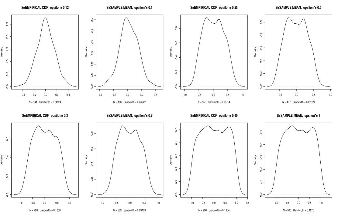
The goal is to compare simulated approximate posteriors of parametric ABC and nonparametric ABC with An ABC example in Tavaré (2019, Lectures at Columbia University, # 2, “A Normal example”, p. 35) is revisited. are normal random variables, The prior for is uniform with and Attention is restricted to the sample mean, since it is sufficient statistic. For fixed the posterior is truncated in For the ABC-simulations and a given it is assumed the observed is observed from and is selected when is absolute value. A flat, “0-1”, kernel is used to select
Approximate posterior densities appear in Figure 1 for nonparametric ABC with and parametric ABC with The Gaussian kernel is used by default in The observed sample is from For the parametric ABC, given tolerance the steps in Tavaré (2019) are followed, using independently of the observed
For nonparametric ABC with is used and is such that the number of selected from does not differ much from that of the parametric ABC. Randomness remains in the simulations but the number of drawn is large, such that the number of selected ( in Figure 1) is also large enough for determining the approximate posterior. is obtained from and is selected if The process is repeated for four values of In Table 2, for the selected their mean variance and the mean square error of from the mean of the posterior are calculated. When and at least 95% of drawn are selected.
| Concentration: Nonparametric ABC with and Parametric ABC with | |||||||
| -nonpar | Mean | Var | MSE | -par | Mean | Var | MSE |
| 0.12 | 0.00456 | 0.022 | 0.022 | 0.1 | 0.01820 | 0.0154 | 0.0157 |
| 0.25 | 0.01780 | 0.119 | 0.119 | 0.5 | -0.00816 | 0.0923 | 0.0924 |
| 0.30 | 0.00774 | 0.192 | 0.192 | 0.6 | -0.01440 | 0.1340 | 0.1340 |
| 0.45 | 0.01990 | 0.332 | 0.332 | 1.0 | 0.01550 | 0.3130 | 0.3130 |
The MSE of parametric ABC posterior improves uniformly in the nonparametric ABC.
3.3 Comparison of parametric ABC with F-ABC
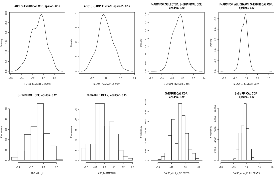
The goal is to compare in simulations parametric ABC with the least favorable for concentration F-ABC, i.e., neglecting the additional concentration due to 3)c) of the F-ABC Algorithm. Remark 2.1 is followed. Start ABC with and and for the selected in ABC, draw additional to compute The F-ABC posterior for these selected is obtained. For the non-selected in ABC, additional are drawn to compute the corresponding The F-ABC posterior for all drawn is then obtained.
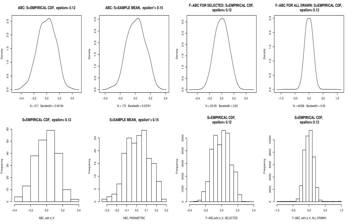
In the simulations, very frequently, the concentration (MSE) of the nonparametric F-ABC improves that of parametric ABC. In Tables 3 and 4 and the corresponding Figures 2 and 3, examples are presented where the MSE of each method dominates the other. The set-up in section 3.2 is used: and For F-ABC, -samples of size are drawn for each selected but also for non-selected A flat, “0-1”, kernel is used for selected in parametric ABC.
In Figures 2 and 3, density plots with Gaussian kernel and corresponding histograms are presented for ABC and F-ABC. For the F-ABC approximate posteriors, the bandwidth was set at 0.05. Nonparametric F-ABC for selected is satisfactory compared with parametric ABC. F-ABC for all seems satisfactory for non-believers of -exclusion with limited -data.
| Concentration: Non Parametric ABC, F-ABC selected/drawn-Parametric ABC | ||||
| Nonparametric , | Parametric, | |||
| Parameter | ABC | F-ABC selected | F-ABC all drawn | ABC |
| Mean | - 0.0916 | -0.0865 | -0.0859 | -0.0117 |
| Variance | 0.0182 | 0.0105 | 0.0274 | 0.0107 |
| MSE | 0.0266 | 0.018 | 0.0348 | 0.0108 |
| Concentration: Non Parametric ABC, F-ABC selected/drawn-Parametric ABC | ||||
| Nonparametric , | Parametric, | |||
| Parameter | ABC | F-ABC selected | F-ABC all drawn | ABC |
| Mean | -0.00198 | -0.00185 | -0.00617 | 0.0112 |
| Variance | 0.0187 | 0.0111 | 0.0242 | 0.0138 |
| MSE | 0.0187 | 0.0111 | 0.0243 | 0.0139 |
To compare the MSE improvement with F-ABC for selected
MSE comparisons555Used for higher accuracy. No need to be repeated. are made
and the total number of times, F-ABC improves ABC is recorded.
The parameters are
The process is repeated 50 times out of which 48 times i.e. F-ABC
for selected improves the MSE of parametric ABC.
A histogram of the results appear in Table 4.
To realize 50 comparisons, the process was repeated 55 times because
of 5 non-terminations since in F-ABC with
there were simulations with no within from
However, in the majority of the remaining cases the number of with F-ABC within
from exceeded that
of ABC.
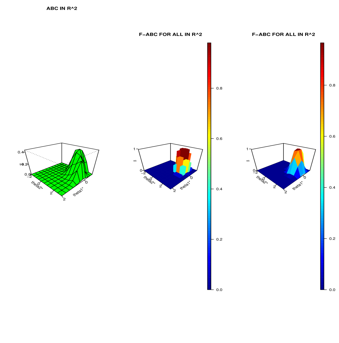
3.4 ABC and F-ABC for all in with and half-spaces
ABC and F-ABC for all, are implemented when with used for - matching over all 1-dimensional projections of and or equivalently in half-spaces, as explained in section 5 for the sufficient, empirical measures
For is the inner product of and is Euclidean distance in Using the notation in section 2, and
are are uniform random vectors in independent of and Direction used in has form with uniform in approximates in (21) when but a moderately large is adequate. For ABC and F-ABC the number of -matching will decrease as increases.
A sample of size is observed from a bivariate normal with means variances and covariance Assume the parameter space is Instead of drawing randomly from a discretization of is used in order to observe the weights along With equidistant and respectively, in and obtain in Following Remark 2.1, to obtain -ABC and -F-ABC posteriors, one sample is drawn initially for each in 50 -directions are used in and 21 match thus selecting 21 from With F-ABC for all without using 3c) in the F-ABC Algorithm, independent copies of are obtained for each For the same 50 -directions and the matchings, in (6) is calculated for and
In Figure 5, the ABC-posterior density and the F-ABC for all posterior histogram and density appear, created with -functions and respectively. Comparison of the ABC and F-ABC densities indicates higher concentration in the latter near the means Outside an area of (0,2), the -values of the densities and the histogram are 0 in all plots. In ABC (all green), the density’s shape and the 0-values in the -axis are due to the bivariate normal kernel used by default in -function needed in In F-ABC for all, no kernel is used: the matching propostions, are the weights, frequencies and percentages, that provide the 0’s and nearly 0-values in the -axis. and cannot be used in F-ABC for the selected
An additional Example is included for the Editors, AE and referees. New parameters are: There are 11 selected with results in Figure 6. The small number of selected in both Examples indicates the ABC-weakness with the choice of -value, which leads to repeated simulations for various until a “satisfactory” posterior is obtained. F-ABC for all does not face this problem, reducing ’s influence.
4 Differences of F-ABC and ABC methods
Main differences, some to appear in section 5, are: the universal sufficient statistics, and and matching via the F-ABC posterior for all drawn or used; the study and choice of the use of for each to obtain which is the -weight and often depends on
For the last difference, in several models it was observed for generic distances that:
| (13) |
| (14) |
Implication (13) usually holds. In F-ABC with when (14) holds it will also hold, at least for large when is replaced by For families of c.d.fs in with densities such that changes sign once, the upper probability of the last implication in (14) increases to 1 with if gets closer to (Yatracos, 2020, Propositions 7.2, 7.4 and Remark 7.2). An inequality similar to (14) holds for the lower bounds of these probabilities (Proposition 5.2). Thus, it is expected the F-ABC approximate posterior concentrates near more than the ABC-posterior, as observed in the simulations in subsections 3.3 and 3.4.
Lemma 4.1
The implications leading to (14) hold for normal random variables with mean and variance 1,
For another difference, is used without loss of generality instead of and measures are Lebesgue measures, each in a Euclidean space. For a function one goal is calculation of
| (15) |
In ABC, (15) is approximated using the selected in
| (16) |
depends on and which is usually intractable or unknown.
5 The Matching tools:
Sufficiency,
In ABC, matching with sufficient is preferred since When is sufficient being equivalent to the order statistic. When and are either or exchangeable, the empirical measure,
| (18) |
is sufficient, respectively by, Dudley (1984, Theorem 10.1.3, p. 95) and de Finetti’s Theorem, e.g., Lauritzen (2007, in Statistical Implications section); are the Borel sets in When for some models may be nearly sufficient but still better than guessing
For to guarantee sufficiency, is used for -matching with As explained below, instead of using for matching the usual form of Total Variation distance,
| (19) |
the supremum in (19) is over all half-spaces,
| (20) |
is the inner product of and is Euclidean distance in Then,
| (21) |
In practice, is approximated by
| (22) |
where are either a discretization of or uniform in independent of and leading to approximate sufficiency. Using in (18),
| (23) |
and the last equalities in (21) and (22) follow, relating over all half-spaces with -distance over all 1-dimensional projections of Hence, in applications, will match when the last term in (22) is less than or equal to with the -functions used for
and
If and are probabilities in which are equal over all half-spaces, in (20), then and are equal for every (Cramér and Wold, 1936). When ’s coordinates follow the unknown probability and is defined in (21), Beran and Millar (1986, p. 431-433, Theorem 3, p. 436) obtained confidence sets for using with uniform on and showed that when as then with probability 1 and asymptotically the required coverage is achieved.
Pertinent properties of
and satisfy desired properties for summary statistics (Fearnhead and Prangle, 2012, Frazier et al., 2018) when is the parameter of interest: a) implies due to identifiability, and c) there are various types of ’s convergence to including -convergence. When and is continuous with respect to and a metric on it is expected that as estimate of will inherit convergence properties of to Similar results hold for the empirical measure, , its corresponding probability and the class of half-spaces which is Vapnik-Cervonenkis class of sets with index (d+1), see, e.g. Dudley (1978).
is not continuous function in at since it cannot be smaller than for all at Euclidean distance from This makes different from other -distances used in ABC, (1), (2); see, e.g. Bernton et al. (2019, p. 39, proof of Proposition 3.1).
Lemma 5.1
For any observed samples of size
| (24) |
denotes a vector, permutation of the components. Thus,
| (25) |
and
For matching support probability in (3), the F-ABC tolerance satisfies
| (26) |
An upper bound on is obtained equating an upper probability bound in (26) with see Lemma 7.1. Conditionally on is similarly obtained under The upper bounds follow for and When similar results hold presented after the Proof of Proposition 5.1.
Proposition 5.1
Let be a sample of random variables from cumulative distribution with unknown, let be a simulated -size sample from a sampler used for
and let be the
matching support probability for the
tolerance in (26);
a) The upper bound for is
| (27) |
b) Conditionally on the upper bound for is
| (28) |
In practice, and are used.
(27) and (28 provide a structure for the tolerance. Since is unknown and uniform upper bounds are useful. Since is with high probability at -distance from a plausible choice for the uniform upper bounds of and is with Probability bounds are rarely tight and, in practice, is determined via simulations; see Table 1 in subsection 3.1.
The next Proposition indicates that for the lower bounds on the Probabilities in (14), the same inequality holds when
Proposition 5.2
For i.i.d. random vectors in with c.d.f. and large:
| (29) |
are positive constants.
6 Asymptotics
Results obtained for Kolmogorov distance, when hold also for the stronger distance (21) using on all half-spaces in
In ABC, one question of interest is whether converges to when stays fixed and as increases.
Proposition 6.1
Use the notation in section 2, for ABC and F-ABC with fixed and in (9). Under the exchangeability assumption, i.e. for any permutation of and with as increases,
| (30) |
For continuous is with the Borel sets, and takes values in
Another question of interest for ABC is whether the posterior will place increasing probability mass around as increases to infinity (Fearnhead, 2018), i.e. Bayesian consistency. Posterior concentration is proved for ABC and F-ABC, initially for fixed size -neighborhood when is the quantity of interest; is a functional,
Proposition 6.2
Use the notation in section 2 and let
be subset of a metric space of c.d.fs. Assume
a)
and -probability as increases,
and
b) is a continuous functional on with values in a metric space
Then,
for
ABC and F-ABC, and for any
| (31) |
| (32) |
Remark 6.1
In Proposition 6.2, assumption a) holds for special case of interest in b) when and the metric on
To confirm Bayesian consistency for shrinking -neighborhoods of let be the modulus of continuity of i.e.
| (33) |
Consistency was established for --neighborhood of when (47) holds, i.e. when
thus it holds for the smallest -value,
| (34) |
and since for --neighborhood of
it follows that
| (35) |
Lemma 6.1
Under the assumptions of Proposition 6.2, the shortest -shrinking neighborhood of for which Bayesian consistency holds has radius
Remark 6.2
The rate of posterior concentration around depends, as expected, on the rate in probability, of the -concentration of around which is not under the user’s control, the tolerance and the modulus of continuity, of Similar conclusions in a different set-up have been obtained by Frazier et al. (2018).
7 Annex
Proof of Lemma 4.1: The first implication holds from the corresponding models, w.l.o.g. for by observing that and comparing with The last implication holds from the assumption since
is decreasing in when and increasing in when and determines the probabilities in (14) for Indeed,
hence if is decreasing in For is increasing,
Proof of Lemma 5.1: The smaller -distance between and occurs when differ by a small in one coordinate of one observation and their distance is
Lemma 7.1
Let and let be positive function defined for positive integers and such that
| (36) |
Let Then
Theorem 7.1
(Dvoretzky, Kiefer and Wolfowitz, 1956, and Massart, 1990, providing the tight constant) Let denote the empirical c.d.f of the size sample of i.i.d. random variables obtained from cumulative distribution Then, for any
| (37) |
Proof of Proposition 5.1: a)
The right side of the last inequality, obtained from (37) is made equal to
b)
obtaining with matching support probability
Generalizations of (37) in have been obtained, at least, by Kiefer and Wolfowitz (1958), Kiefer (1961) and Devroye (1977); The differences in upper bound in (37) are in the multiplicative constant, in the exponent of the exponential and on the sample size for which the exponential bound holds which may also depend on The constants used are not determined except for Devroye (1977).
For example, following the Proof in Proposition 5.1 b), conditionally on
i) Using Kiefer and Wolfowitz (1958),
with the upper bound in (37)
ii) Using Kiefer (1961), with the upper bound in (37) for every
iii) Using Devroye (1977), with the upper bound in (37) valid for
Remark 7.1
Proof of Proposition 5.2: Follows along the first three lines in the proof of Proposition 5.1 a), with the exponential upper bound obtained using the above in i) (Kiefer and Wolfowitz, 1958), with the adjustments of
Proof of Proposition 6.1: The arguments used for ABC hold for F-ABC.
a) discrete: The ABC posterior with in (10) is
With integral denoting sum, it is enough to prove that the integral in the numerator of is proportional to
For let
is a probability measure on
Since and are fixed, for
| (38) |
and from Lemma 5.1 for Therefore,
| (39) |
and
| (40) |
with the last equality due to exchangeability of
b) continuous: Then, the right side of (40) vanishes, since A different approach is used, via the notion of regular conditional probability.
When is a Euclidean space with Borel -field, and takes values in the integral in the numerator of
is a regular conditional probability, (Breiman, 1992, Chapter 4, p. 79, Theorem 4.34), i.e., with fixed, it is a probability for and with fixed it is a version of the conditional density, Thus, for fixed from (39),
and due to exchangeability is proportional to a.s. .
Proof of Proposition 6.2: The arguments used for ABC hold for F-ABC.
For the probability in (31), using
(11) for ABC
with
| (41) |
| (42) |
in the numerators of (42) will be bounded below using continuity of and triangular inequality.
Since is continuous, for there is such that if
| (43) |
Since
| (44) |
if
and therefore, for the right side of (43)
| (45) |
From the assumptions,
with and probabilities converging to one, respectively, and assuming are in these subsets the right side of (45)
| (46) |
For as increases, eventually
| (47) |
and the right side of (46)
| (48) |
(31) follows from (43), (45)-(48) since, when taking the limit in (42) as increases to infinity, for large numerator and denominator coincide.
Acknowledgments
Many thanks are due to Professor Rudy Beran for communicating pertinent useful results in his 1986 paper with Professor Warry Millar.
References
- [1] Beran, R. and Millar, P. W. (1986) Confidence Sets for a Multivariate Distribution. Ann. Statist. 14, 431-443.
- [2] Bornn, L., Pillai, N. S., Smith, A. and Woodard, D. (2017) The Use of a Single Pseudo-Sample in Approximate Bayesian Computation. Stat. and Comput. 27, 583-590.
- [3] Bernton, E. , Jacob, P. E., Gerbery, M. and Robert, C. P. (2019) Approximate Bayesian computation with the Wasserstein distance. arXiv:1905.03747v1
- [4] Biau, G., Cérou, F. and Guyader, A. (2015) New insights into approximate Bayesian computation. Annales de l’ IHP (Probab. Stat.) 51, 376-403
- [5] Breiman, L. (1992) Probability Classics in Applied Mathematics, SIAM.
- [6] Cramér, H. and Wold, H. (1936) Some theorems on distribution functions.J. London Math. Soc. 11, 290-294.
- [7] Devroye, L. P. (1977) A Uniform Bound for the Deviation of Empirical Distribution Functions. J. Multiv. Anal. 7, 594-597.
- [8] Dudley, R. M. (1984) A course on empirical processes. École d’ Été de Probabilités de St. Flour. Lecture Notes in Math. 1097, 2-142, Springer Verlag, New York.
- [9] Dudley, R. M. (1978) Central limit theorem for empirical measures. Ann. Prob. 6, 899-929.
- [10] Dvoretzky, A., Kiefer, J. and and Wolfowitz, J. (1956) Asymptotic minimax character of the sample distribution function and of the classical multinomial estimator. Ann. Math. Stat. 27, 642-669
- [11] Fearnhead, P. (2018) Asymptotics of ABC. Handbook of Approximate Bayesian Computation, Editor:Routledge Handbooks Online.
- [12] Fearnhead, P. and Prangle, D. (2012) Constructing summary statistics for approximate Bayesian computation: semi-automatic approximate Bayesian computation. J. R. Statist. Soc. B 74, 419-474.
- [13] Frazier, D. T., Martin, G. M., Robert, C. P. and Rousseau, J. (2018) Asymptotic properties of approximate Bayesian Computation. Biometrika 105, 593-607.
- [14] Frazier, D. T., Martin, G. M. and Robert, C. P. (2015) On Consistency of Approximate Bayesian Computation arXiv:1508.05178v1
- [15] Kiefer, J. (1961) On Large Deviations of the Empiric D. F. of Vector Chance Variables and a Law of the Iterated logarithm. Pacific J. of Mathematics 11, 649-660
- [16] Kiefer, J. and Wolfowitz, J. (1958) On the deviations of the empiric distribution function of vector chance variables. Trans. Amer. Math. Soc. 87, 173-186
-
[17]
Lauritzen, S. (2007) Exchangeability and de Finetti’s Theorem. Lecture Notes, University of Oxford,
http://www.stats.ox.ac.uk/steffen/teaching/grad/definetti.pdf - [18] Lintusaari, J., Gutmann, M. U., Dutta, R., Kaski, S. and Corander, J. (2017) Fundamentals and Recent Developments in Approximate Bayesian Computation. Syst. Biol. 66, e66-e82.
- [19] Massart, P. (1990) The tight constant in the Dvoretzky-Kiefer-Wolfowitz inequality. Ann. Prob. 18, 1269-1283
- [20] Miller, J. W. and Dunson, D. B. (2019) Robust Bayesian inference via coarsening. J. Am. Stat. Assoc. 114, 1113-1125
- [21] Nott, D. J., Drovandi, C. C., Mengersen, K. and Evans, M. (2018) Approximation of Bayesian Predictive p-Values with Regression ABC. Bayesian Analysis 13, 59-83.
- [22] Pritchard, J. K., Seilstad, M. T., Perez-Lezaun, A and Feldman, M. W. (1999) Population Growth of Human Y Chromosomes: A Study of Y Chromosome Microsatellites. Molecular Biology and Evolution, 16, 1791-1798.
- [23] Robert C.P. (2016) Approximate Bayesian Computation: A Survey on Recent Results. In: Cools R., Nuyens D. (eds) Monte Carlo and Quasi-Monte Carlo Methods. Springer Proceedings in Mathematics & Statistics, vol 163. Springer, Cham
- [24] Rubin, D. B. (2019) Conditional Calibration and the Sage Statistician. Survey Methodology 45, 187-198.
- [25] Rubin, D. B. (1984) Bayesianly Justifiable and Relevant Frequency Calculations for the Applied Statistician. Ann. Statist. 12, pp. 213-244.
- [26] Tanaka, M.M., Francis, A. R., Luciani, F. and Sisson, S. A. (2006) Using Approximate Bayesian Computation to Estimate Tuberculosis Transmission Parameters From Genotype Data. Genetics, 173, 1511–1520.
- [27] Tavaré, S. (2019). An introduction to Approximate Bayesian Computation. Summer Program, Herbert and Florence Irving Institute for Cancer Dynamics. https://cancerdynamics.columbia.edu/content/summer-program
- [28] Tavaré, S., Balding, D. J., Griffiths, R. C. and Donnelly, P. (1997). Inferring Coalescence Times from DNA Sequence Data, Genetics, 145, 505-518.
- [29] Vihola, M. and Franks, J. (2020) On the use of approximate Bayesian computation Markov chain Monte Carlo with inflated tolerance and post correction. Biometrika https://doi.org/10.1093/biomet/asz078
- [30] Yatracos, Y. G. (2020) Matching Estimation for Data Generating Experiments. Preprint