On the generalization of Tanimoto-type kernels to real valued functions

Abstract

The Tanimoto kernel (Jaccard index) is a well known tool to describe the similarity between sets of binary attributes. It has been extended to the case when the attributes are nonnegative real values. This paper introduces a more general Tanimoto kernel formulation which allows to measure the similarity of arbitrary real-valued functions. This extension is constructed by unifying the representation of the attributes via properly chosen sets. After deriving the general form of the kernel, explicit feature representation is extracted from the kernel function, and a simply way of including general kernels into the Tanimoto kernel is shown. Finally, the kernel is also expressed as a quotient of piecewise linear functions, and a smooth approximation is provided.

1 Introduction

In a broad range of machine learning, pattern recognition and data mining problems the data sources are given as sets of simple, mostly binary attributes. These sets are generally represented by indicator functions. An element of the feature set corresponding to an attribute is given by a class, and that element expresses that the data object is a member of that class or not. Using this data representation, we can derive similarity or dissimilarity measures between objects. Several of those similarity measures can be formulated as positive definite inner products, thus they can serve as kernel functions of a Reproducing Kernel Hilbert space, [1]. A well known instance of these type of measures is the Jaccard index, which was introduced by [2]. That index is a normalized measure, thus decreases the effect caused by the different sizes of the sets, which otherwise could distort the comparison. The Jaccard index has been extended beyond the case of the indicator function represented sets by allowing nonnegative, real-valued feature vectors. This extension is generally referred to as weighted Jaccard index [3]. When the Jaccard index is used as a kernel function then it is generally called as Tanimoto kernel honoring its first application by [4]. The kernel derived from the weighted Jaccard index is also referred to as MinMax kernel, [3].

These type of similarity measures, or kernels, are extensively used in bio- and chemoinformatics. One of the most general application relates to the representation of molecules which uses, so called, molecular fingerprints. These fingerprints enumerate the occurrences of the characteristic substructures in the molecules. We can mention here only a few but illustrative examples of the applications: [5], [6], [7], [8], [9], [10], [11] and [12].

The purpose of this paper is to extend the known Tanimoto kernels (Jaccard indexes) to the case where the objects are represented by arbitrary real-valued vectors or functions. We present the derivation of the generalized Tanimoto kernel and its relationship to the previously known variants. Figure 1 illustrates the gradual extension of the application domain of the Tanimoto kernel.

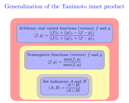
Figure 1: The summary of the levels generalizing the inner product defining the Tanimoto kernel.

1.1 Notations

$\mathbb{R}_{+}$ denotes the set of nonnegative real numbers. Let $S$ be a set, and its power set is denoted by $2^{S}$. $|S|$ is the size of the set $S$. In this paper we assume that $|S|$ is finite. The inner product between two functions $f,g:\mathcal{D}\mapsto\mathbb{R}$ with respect to a finite measure $\mu$ defined on the domain $\mathcal{D}$ is given by $\int\limits_{x\in\mathcal{D}}f(x)g(x)d\mu(x)$. In the sequel we assume that for every function $f$ mentioned $|f|$ is bounded. The finite dimensional vectors are taken as piecewise constant functions.

The $L_{1}$ norm of a function $f:\mathcal{D}\rightarrow\mathbb{R}$ is equal to $\|f\|_{1}=\int\limits_{x\in\mathcal{D}}|f(x)|dx$ assuming that the integral is finite. The $L_{1}$ norm can be generalized by taking the integral with respect to the a nonnegative, finite measure $\mu$, i.e. $\|f\|_{1_{\mu}}=\int\limits_{x\in\mathcal{D}}|f(x)|d\mu(x)$.

2 Kernels on sets

Let $\mathcal{D}$ be a set. A set system $\mathscr{X}$ is defined as a subset of the power set $2^{\mathcal{D}}$, i.e. a set of subsets of $\mathcal{D}$. We assume that $\mathscr{X}$ is a set algebra, thus it is closed on countable infinite intersections and unions, namely for finite examples all $A\in\mathscr{X}$ and $B\in\mathscr{X}$ , $A\cap B\in\mathscr{X}$ and $A\cup B\in\mathscr{X}$. Furthermore for every subset $S\in\mathscr{X}$ $\mathcal{D}\setminus S\in\mathscr{X}$ holds. The set $\mathcal{D}$, consequently the $\emptyset$, is in $\mathscr{X}$ as well. We might also assume that if $\mathcal{D}$ is finite set then for all $x\in\mathcal{D}$ the singleton set $\{x\}$ is in $\mathscr{X}$ as well.

Suppose that there is a finite measure $\mu$ defined on $\mathcal{D}$, i.e. $\mu(\mathcal{D})<\infty$, and all elements of $\mathscr{X}$ are measurable with a positive measure except for the $\emptyset$. If $I_{A}$ denotes the indicator function of a subset $A$ of $\mathcal{D}$ and $A\in\mathscr{X}$ then $\mu(A)=\int\limits_{x\in\mathcal{D}}I_{A}(x)d\mu(x)$. If $\mathcal{D}$ is a finite set, $\mu$ might be defined as a counting measure on the singletons.

We can define a positive definite inner product between sets, and rely on those inner products to develop kernel based machine learning methods. For more background and several other alternative realizations refer to the book [1]. The examples mentioned here can only demonstrate the broad range of possible kernels defined on sets. For us the following two cases are important. Let $A,B\in\mathscr{X}$ be arbitrary sets, then we can define these kernels:

• Intersection kernel: The basic case assuming a counting measure is given by

  $$\kappa_{\cap}(A,B)=|A\cap B|,$$ (1)

  and the general case can be written in this form

  $$\begin{array}[]{ll}\kappa_{\cap}(A,B)_{\mu}&=\mu(A\cap B)=\int\limits_{x\in\mathcal{D}}I_{A\cap B}(x)d\mu(x)=\int\limits_{x\in\mathcal{D}}I_{A}(x)I_{B}(x)d\mu(x)\\ &=\braket{I_{A}(x),I_{B}(x)}_{\mu}.\end{array}$$ (2)

• Tanimoto kernel: The counting measure based version is given by

  $$\kappa_{tanimoto}(A,B)=\dfrac{|A\cap B|}{|A\cup B|},$$ (3)

  and the case relating to a general measure $\mu$ is the following

  $$\kappa_{tanimoto}(A,B)_{\mu}=\dfrac{\mu(A\cap B)}{\mu(A\cup B)}=\dfrac{\int\limits_{x\in\mathcal{D}}I_{A\cap B}(x)d\mu(x)}{\int\limits_{x\in\mathcal{D}}I_{A\cup B}(x)d\mu(x)}.$$ (4)

In the sequel, for sake of simplicity the subscript _μ might be dropped from the notation of the kernels whenever it is clear which measure is applied.

3 Main results

In this Section a summary of the results are presented. We start with the known extension of the Tanimoto kernel constructed on the nonnegative functions, i.e. $f:\mathcal{D}\rightarrow\mathbb{R}_{+}$ (c.f. [3]), and subsequently present the generalized version for the arbitrary real-valued case. The details of the derivation are unfolded in the following Section 4.

3.1 Nonnegative functions

We can represent a nonnegative function $f$ using a set based description. Let $A_{f}$ be a set assigned to $f$, and it is defined by:

$$A_{f}=\{(x,y)|x\in\mathcal{D},y\in\mathbb{R},0\leq y\leq f(x)\}\subset\mathcal{D}\times\mathbb{R}.$$ (5)

The set $A_{f}$ represents the area between the graph of the function and the $x$ axes. For a pair of nonnegative functions $f$ and $g$ we can define the extended intersection and the Tanimoto kernels utilizing the set based description.

Proposition 1.

For any nonnegative functions $f$ and $g$ defined on the domain $\mathcal{D}$, and for the finite measure $\mu$ we have the intersection kernel

$$\kappa_{\cap}(f,g)=\mu(A_{f}\cap A_{g})=\int\limits_{x\in\mathcal{D}}\min(f(x),g(x))d\mu(x),$$ (6)

and the Tanimoto kernel

$$\kappa(f,g)_{tanimoto}=\dfrac{\mu(A_{f}\cap A_{g})}{\mu(A_{f}\cup A_{g})}=\dfrac{\int\limits_{x\in\mathcal{D}}\min(f(x),g(x))d\mu(x)}{\int\limits_{x\in\mathcal{D}}\max(f(x),g(x))d\mu(x)}.$$ (7)

This kernel is generally referred as MinMax kernel, see for example [3].

3.2 Arbitrary real-valued functions

Now we move on to the main result of this paper. For the general case we need to extend the definition of the set $A_{f}$ assigned to an arbitrary real valued function $f:\mathcal{D}\rightarrow\mathbb{R}$. To this end we split the domain $\mathcal{D}$ of $f$ based on the sign of the function values. Let $f=f^{+}+f^{-}$ where

$$\begin{array}[]{ll}f^{+}(x)=\left\{\begin{array}[]{ll}f(x)&f(x)\geq 0,\\ 0&f(x)<0,\end{array}\right.&f^{-}(x)=\left\{\begin{array}[]{ll}-f(x)&f(x)<0,\\ 0&f(x)\geq 0.\end{array}\right.\end{array}$$ (8)

Clearly, $f^{+}$ and $(-f)^{-}$ are nonnegative functions. Let

$$\begin{array}[]{@{}ll@{}}A^{+}_{f}&=\{(x,y)|x\in\mathcal{D},y\in\mathbb{R},0\leq y\leq f^{+}(x)\},\end{array}$$ (9)

and

$$\begin{array}[]{@{}ll@{}}A^{-}_{f}&=\{(x,y)|x\in\mathcal{D},y\in\mathbb{R},\ f^{-}(x)\leq y<0\},\end{array}$$ (10)

be the corresponding sets. Note that $A^{+}_{f}\cap A^{-}_{f}=\emptyset$, and we can define $A_{f}$ as

$$A_{f}=A^{+}_{f}\cup A^{-}_{f}.$$ (11)

We can construct the corresponding kernels for the general case.

Proposition 2.

Let $f$ and $g$ be any real valued functions on domain $\mathcal{D}$, and for the finite measure $\mu$ we have the intersection kernel

$$\begin{array}[]{@{}l@{\:}l@{}}\kappa_{\cap}(f,g)\hfil\>&=\mu(A_{f}\cap A_{g})=\frac{1}{2}(\|f\|_{1_{\mu}}+\|g\|_{1_{\mu}}-\|f-g\|_{1_{\mu}})\\ \hfil\>&=\int\limits_{\min(f(x),g(x))\geq 0}\min(f(x),g(x))d\mu(x)-\int\limits_{\max(f(x),g(x))<0}\max(f(x),g(x))d\mu(x).\end{array}$$ (12)

and the Tanimoto kernel

$$\begin{array}[]{@{}l@{\:}l@{}}\kappa_{tanimoto}(f,g)\hfil\>&=\dfrac{\mu(A_{f}\cap A_{g})}{\mu(A_{f}\cup A_{g})}=\dfrac{\frac{1}{2}(\|f\|_{1_{\mu}}+\|g\|_{1_{\mu}}-\|f-g\|_{1_{\mu}})}{\frac{1}{2}(\|f\|_{1_{\mu}}+\|g\|_{1_{\mu}}+\|f-g\|_{1_{\mu}})}\\ \hfil\>&=\dfrac{\int\limits_{\min(f(x),g(x))\geq 0}\min(f(x),g(x))d\mu(x)-\int\limits_{\max(f(x),g(x))<0}\max(f(x),g(x))d\mu(x)}{\int\limits_{\max(f(x),g(x))\geq 0}\max(f(x),g(x))d\mu(x)-\int\limits_{\min(f(x),g(x))<0}\min(f(x),g(x))d\mu(x)}.\end{array}$$ (13)

4 Background

In Section 3 to a function $f$ we assign a set $A_{f}$ defined on the area between the graph of the function and the $X$-axis. Here we show a slightly different approach to define the same $A_{f}$ which allows to reformulate the expression (13) of the general Tanimoto kernel. In the description of the alternative form we exploit the concept of epigraph of a function. The epigraph and plays a central role in convex analysis, [13], and in the variational analysis of general functions, and multi-valued mappings, [14].

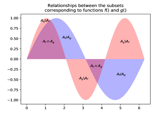
Figure 2: The interrelations of the areas, $A_{f}$ and $A_{g}$, defined via the functions $f$ and $g$.

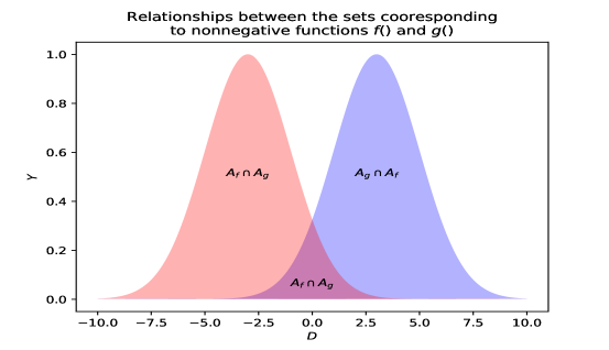
Figure 3: The interrelations of the areas, $A_{f}$ and $A_{g}$, defined via the non-negative functions $f$ and $g$.

We define a function in the same way, $f:\mathcal{D}\rightarrow\mathbb{R}$, as we did earlier. The epigraph of $f$ is a set and given by

$$\mathscr{E}_{f}=\{(x,y)|y\geq f(x),x\in\mathcal{D}\}.$$ (14)

The graph of a function is the set

$$\mathscr{G}_{f}=\{(x,y)|y=f(x),x\in\mathcal{D}\}.$$ (15)

The hypograph of $f$ of is equal to

$$\mathscr{H}_{f}=\{(x,y)|y\leq f(x),x\in\mathcal{D}\}=\mathscr{G}_{f}\cup\mathscr{E}_{f},$$ (16)

which is a complement of the epigraph which also comprises the graph of the function. For any pair of bounded functions $f$ and $g$ based on the definition of the epigraph and hypograph we can derive these equations

$$\begin{array}[]{llll}\mathscr{H}_{f}\cap\mathscr{H}_{g}&=\mathscr{H}_{\min(f,g)},&\mathscr{E}_{f}\cap\mathscr{E}_{g}&=\mathscr{E}_{\max(f,g)},\\ \mathscr{H}_{f}\cup\mathscr{H}_{g}&=\mathscr{H}_{\max(f,g)},&\mathscr{E}_{f}\cap\mathscr{E}_{g}&=\mathscr{E}_{\min(f,g)}.\\ \end{array}$$ (17)

Assuming that the measure $\mu$ is finite, and $f$ is bounded from above and below, we also have the following statements.

• For any $f$ we have $\mu_{\mathcal{D}\times\mathbb{R}}(\mathcal{G}_{f})=0$.

• As a consequence $\mu_{\mathcal{D}\times\mathbb{R}}(\mathcal{E}_{f}\cap\mathcal{H}_{f})=0$ holds as well.

• Another consequence in case of any sets $A,B\subset\mathcal{D}\times\mathbb{R}$

  $$\mu_{\mathcal{D}\times\mathbb{R}}((A\cap B\cap\mathcal{E}_{f}\cap\mathcal{H}_{f}))=0$$ (18)

  is also true, since $A\cap B\cap\mathcal{E}_{f}\cap\mathcal{H}_{f}\subseteq\mathcal{E}_{f}\cap\mathcal{H}_{f}$.

With these concepts at hand we can redefine $A_{f}$ as $A_{f}=(\mathscr{H}_{f}\cap\mathscr{E}_{0})\cup(\mathscr{E}_{f}\cap\mathscr{H}_{0})$, where $\mathcal{E}_{0}$ is the epigraph of the constant, $0$ valued function. Note that the redefined $A_{f}$ covers the same set as earlier. For sake of simplicity, in the following expression we might drop the intersection operator $\cap$, thus for any sets $A$ and $B$, $AB$ means $A\cap B$. If two functions $f$ and $g$ are given on the same domain, the intersection of the corresponding sets is

$$\begin{array}[]{ll}A_{f}\cap A_{g}&=(\mathscr{H}_{f}\mathscr{E}_{0}\cup\mathscr{E}_{f}\mathscr{H}_{0})(\mathscr{H}_{g}\mathscr{E}_{0}\cup\mathscr{E}_{g}\mathscr{H}_{0})\\ &=\mathscr{H}_{f}\mathscr{H}_{g}\mathscr{E}_{0}\cup\mathscr{E}_{f}\mathscr{H}_{g}\mathscr{H}_{0}\mathscr{E}_{0}\cup\mathscr{H}_{f}\mathscr{E}_{g}\mathscr{E}_{0}\mathscr{H}_{0}\cup\mathscr{E}_{f}\mathscr{E}_{g}\mathscr{H}_{0}.\end{array}$$ (19)

Exploiting the equality (18), we can see that the terms containing the intersection $\mathscr{E}_{0}\cap\mathscr{H}_{0}$ have to have $0$ measure with respect to $\mu_{\mathcal{D}\times\mathbb{R}}$. Hence we can state that

$$\begin{array}[]{@{}l@{\:}l@{}}\mu_{\mathcal{D}\times\mathbb{R}}(A_{f}\cap A_{g})\hfil\>&=\mu_{\mathcal{D}\times\mathbb{R}}(\mathscr{H}_{f}\mathscr{H}_{g}\mathscr{E}_{0})+\mu_{\mathcal{D}\times\mathbb{R}}(\mathscr{E}_{f}\mathscr{E}_{g}\mathscr{H}_{0})\\ \hfil\>&=\int\limits_{\begin{subarray}{c}x\in\mathcal{D}\\ \min(f(x),g(x))\geq 0\end{subarray}}\min(f(x),g(x))d\mu(x)-\int\limits_{\begin{subarray}{c}x\in\mathcal{D}\\ \max(f(x),g(x))<0\end{subarray}}\max(f(x),g(x))d\mu(x).\end{array}$$ (20)

In case of the union of $A_{f}$ and $A_{g}$, we can similarly write

$$\begin{array}[]{ll}A_{f}\cup A_{g}&=\mathscr{H}_{f}\mathscr{E}_{0}\cup\mathscr{E}_{f}\mathscr{H}_{0}\cup\mathscr{H}_{g}\mathscr{E}_{0}\cup\mathscr{E}_{g}\mathscr{H}_{0}\\ &=(\mathscr{H}_{f}\cup\mathscr{H}_{g})\mathscr{E}_{0}\cup(\mathscr{E}_{f}\cup\mathscr{E}_{g})\mathscr{H}_{0}.\end{array}$$ (21)

By applying (18) again, the intersection of $(\mathscr{H}_{f}\cup\mathscr{H}_{g})\mathscr{E}_{0}$ and $(\mathscr{E}_{f}\cup\mathscr{E}_{g})\mathscr{H}_{0}$ has zero measure with respect to $\mu_{\mathcal{D}\times\mathbb{R}}$. Therefore we have

$$\begin{array}[]{ll}\mu_{\mathcal{D}\times\mathbb{R}}(A_{f}\cup A_{g})&=\mu_{\mathcal{D}\times\mathbb{R}}((\mathscr{H}_{f}\cup\mathscr{H}_{g})\mathscr{E}_{0})+\mu_{\mathcal{D}\times\mathbb{R}}((\mathscr{E}_{f}\cup\mathscr{E}_{g})\mathscr{H}_{0})\\ &=\int\limits_{\begin{subarray}{c}x\in\mathcal{D}\\ \max(f(x),g(x))\geq 0\end{subarray}}\max(f(x),g(x))d\mu(x)-\int\limits_{\begin{subarray}{c}x\in\mathcal{D}\\ \min(f(x),g(x))<0\end{subarray}}\min(f(x),g(x))d\mu(x).\end{array}$$ (22)

The underlying geometry of the general case is highlighted on Figure 2. Figure 3 demonstrates the simpler geometric setting exploited in the case of nonnegative functions.

Now we can express the general Tanimoto kernel by exploiting the equations of (17) connecting the pointwise minimum and maximum of functions to the intersection of epigraphs and the hypographs.

$$\begin{array}[]{ll}\kappa_{tanimoto}(f,g)=\dfrac{\mu(A_{f}\cap A_{g})}{\mu(A_{f}\cup A_{g})}\\ \quad=\dfrac{\int\limits_{\min(f(x),g(x))\geq 0}\min(f(x),g(x))d\mu(x)-\int\limits_{\max(f(x),g(x))<0}\max(f(x),g(x))d\mu_{\mathcal{D}}(x)}{\int\limits_{\max(f(x),g(x))\geq 0}\max(f(x),g(x))d\mu_{\mathcal{D}}(x)-\int\limits_{\min(f(x),g(x))<0}\min(f(x),g(x))d\mu_{\mathcal{D}}(x)}\end{array}$$ (23)

Both in the numerator and the denominator within the second terms we can use strict inequalities defining the integral domain, since the integrals of bounded functions on the boundaries of the integral domains are equal to $0$.

In the remaining part of this section we show that the generalized Tanimoto kernel can also be described by the help of $L_{1}$ norm. We have the following statements.

Proposition 3.

For any functions $f,g:\mathcal{D}\rightarrow\mathbb{R}$ we have for the intersection

$$\begin{array}[]{ll}\frac{1}{2}(||f||_{1_{\mu}}+||g||_{1_{\mu}}-||f-g||_{1_{\mu}})\\ \qquad=\int\limits_{\min(f(x),g(x))\geq 0}\min(f(x),g(x))d\mu_{\mathcal{D}}(x)-\int\limits_{\max(f(x),g(x))<0}\max(f(x),g(x))d\mu_{\mathcal{D}}(x)\\ \qquad=\mu(A_{f}\cap A_{g}),\end{array}$$ (24)

and for the union

$$\begin{array}[]{ll}\frac{1}{2}(||f||_{1_{\mu}}+||g||_{1_{\mu}}+||f-g||_{1_{\mu}})\\ \qquad=\int\limits_{\max(f(x),g(x))\geq 0}\max(f(x),g(x))d\mu_{\mathcal{D}}(x)-\int\limits_{\min(f(x),g(x))<0}\min(f(x),g(x))d\mu_{\mathcal{D}}(x)\\ \qquad=\mu(A_{f}\cup A_{g}).\end{array}$$ (25)

Proof.

By inspection for any $x\in\mathcal{D}$ we can claim the following identities

$$\begin{array}[]{lll}f(x)+g(x)&=\max(f(x),g(x))+\min(f(x),g(x)),\\ f(x)-g(x)&=\max(f(x),g(x))-\min(f(x),g(x)),&\text{if}\ f(x)\geq g(x),\\ |f(x)-g(x)|&=\max(f(x),g(x))-\min(f(x),g(x)).\\ \end{array}$$ (26)

The sub-terms of the $L_{1}$ norm based forms can be expressed by the help of the minimum and maximum functions.

$$\begin{array}[]{ll}||f-g||_{1_{\mu}}&=\int\limits_{x\in\mathcal{D}}|f(x)-g(x)|d\mu(x)\\ &=\int\limits_{x\in\mathcal{D}}\left(\max(f(x),g(x))-\min(f(x),g(x))\right)d\mu(x)\\ &=+\int\limits_{\begin{subarray}{c}x\in\mathcal{D}\\ \max(f(x),g(x))\geq 0\end{subarray}}\max(f(x),g(x)d\mu(x)+\int\limits_{\begin{subarray}{c}x\in\mathcal{D}\\ \max(f(x),g(x))<0\end{subarray}}\max(f(x),g(x)d\mu(x)\\ &\quad-\int\limits_{\begin{subarray}{c}x\in\mathcal{D}\\ \min(f(x),g(x))\geq 0\end{subarray}}\min(f(x),g(x)d\mu(x)-\int\limits_{\begin{subarray}{c}x\in\mathcal{D}\\ \min(f(x),g(x))<0\end{subarray}}\min(f(x),g(x)d\mu(x)\\ &=+\int\limits_{\begin{subarray}{c}x\in\mathcal{D}\\ \max(f(x),g(x))\geq 0\end{subarray}}\max(f(x),g(x)d\mu(x)-\int\limits_{\begin{subarray}{c}x\in\mathcal{D}\\ \min(f(x),g(x))<0\end{subarray}}\min(f(x),g(x)d\mu(x)\\ &\quad-\int\limits_{\begin{subarray}{c}x\in\mathcal{D}\\ \min(f(x),g(x))\geq 0\end{subarray}}\min(f(x),g(x)d\mu(x)+\int\limits_{\begin{subarray}{c}x\in\mathcal{D}\\ \max(f(x),g(x))<0\end{subarray}}\max(f(x),g(x)d\mu(x)\\ &=\mu(A_{f}\cup A_{g})-\mu(A_{f}\cap A_{g})\end{array}$$ (27)

The sum of the $L_{1}$ norms can be expressed by

$$\begin{array}[]{@{}l@{\:}l@{}}||f||_{1_{\mu}}+||g||_{1_{\mu}}\hfil\>&=\int\limits_{x\in\mathcal{D}}|f(x)|+|g(x)|d\mu(x)\\ \hfil\>&=+\int\limits_{\begin{subarray}{c}x\in\mathcal{D}\\ f(x)\geq 0,g(x)\geq 0,\end{subarray}}f(x)+g(x)d\mu(x)-\int\limits_{\begin{subarray}{c}x\in\mathcal{D}\\ f(x)<0,g(x)<0,\end{subarray}}f(x)+g(x)d\mu(x)\\ \hfil\>&\quad+\int\limits_{\begin{subarray}{c}x\in\mathcal{D}\\ f(x)\geq 0,g(x)<0,\end{subarray}}f(x)-g(x)d\mu(x)+\int\limits_{\begin{subarray}{c}x\in\mathcal{D}\\ f(x)<0,g(x)\geq 0,\end{subarray}}g(x)-f(x)d\mu(x)\\ \hfil\>&=+\int\limits_{\begin{subarray}{c}x\in\mathcal{D}\\ f(x)\geq 0,g(x)\geq 0,\end{subarray}}\max(f(x),g(x))+\min(f(x),g(x))d\mu(x)\\ \hfil\>&\quad-\int\limits_{\begin{subarray}{c}x\in\mathcal{D}\\ f(x)<0,g(x)<0,\end{subarray}}\max(f(x),g(x))+\min(f(x),g(x))d\mu(x)\\ \hfil\>&\quad+\int\limits_{\begin{subarray}{c}x\in\mathcal{D}\\ f(x)\geq 0,g(x)<0,\end{subarray}}\max(f(x),g(x))-\min(f(x),g(x))d\mu(x)\\ \hfil\>&\quad+\int\limits_{\begin{subarray}{c}x\in\mathcal{D}\\ f(x)<0,g(x)\geq 0,\end{subarray}}\max(f(x),g(x))-\min(f(x),g(x))d\mu(x).\\ \end{array}$$ (28)

By applying these identities

$$\begin{array}[]{@{}l@{\:}l@{}}\{x|\max(f(x),g(x))\geq 0\}=\{x|f(x)\geq 0,g(x)\geq 0\}\cup\{x|f(x)\geq 0,g(x)<0\}\cup\{x|f(x)<0,g(x)\geq 0\},\hfil\>\\ \{x|\max(f(x),g(x))<0\}=\{x|f(x)<0,g(x)<0\},\hfil\>\\ \{x|\min(f(x),g(x))\geq 0\}=\{x|f(x)\geq 0,g(x)\geq 0\},\hfil\>\\ \{x|\min(f(x),g(x))<0\}=\{x|f(x)<0,g(x)<0\}\cup\{x|f(x)\geq 0,g(x)<0\}\cup\{x|f(x)<0,g(x)\geq 0\},\hfil\>\\ \end{array}$$ (29)

we can rearrange the terms in (28), which gives us

$$\begin{array}[]{@{}l@{\:}l@{}}||f||_{1_{\mu}}+||g||_{1_{\mu}}\hfil\>&=+\int\limits_{\begin{subarray}{c}x\in\mathcal{D}\\ \max(f(x),g(x))\geq 0\end{subarray}}\max(f(x),g(x)d\mu(x)-\int\limits_{\begin{subarray}{c}x\in\mathcal{D}\\ \min(f(x),g(x))<0\end{subarray}}\min(f(x),g(x)d\mu(x)\\ \hfil\>&\quad-\int\limits_{\begin{subarray}{c}x\in\mathcal{D}\\ \min(f(x),g(x))\geq 0\end{subarray}}\min(f(x),g(x)d\mu(x)+\int\limits_{\begin{subarray}{c}x\in\mathcal{D}\\ \max(f(x),g(x))<0\end{subarray}}\max(f(x),g(x)d\mu(x)\\ \hfil\>&=\mu(A_{f}\cup A_{g})-\mu(A_{f}\cap A_{g}).\end{array}$$ (30)

After combining the sub-terms together, we can arrive at the final formulas. For the intersection we have

$$\begin{array}[]{ll}\frac{1}{2}(||f||_{1_{\mu}}+||g||_{1_{\mu}}-||f-g||_{1_{\mu}})&=\frac{1}{2}(\mu(A_{f}\cup A_{g})-\mu(A_{f}\cap A_{g})-\mu(A_{f}\cup A_{g})+\mu(A_{f}\cap A_{g}))\\ &=\mu(A_{f}\cap A_{g})),\end{array}$$ (31)

and the union takes this form

$$\begin{array}[]{ll}\frac{1}{2}(||f||_{1_{\mu}}+||g||_{1_{\mu}}+||f-g||_{1_{\mu}})&=\frac{1}{2}(\mu(A_{f}\cup A_{g})-\mu(A_{f}\cap A_{g})+\mu(A_{f}\cup A_{g})-\mu(A_{f}\cap A_{g}))\\ &=\mu(A_{f}\cup A_{g})).\end{array}$$ (32)

∎

From Proposition 3 we can straightforwardly derive the MinMax kernel for the nonnegative functions, see in Proposition 7. If the functions are nonnengative then the second terms in both the numerator and the denominator of (23) can be dropped.

Corollary 4.

For any nonnegative functions $f,g:\mathcal{D}\rightarrow\mathbb{R}$ the generalized Tanimoto kernel takes the following form

$$\begin{array}[]{ll}\kappa_{\cap}(f,g)=\mu(A_{f}\cap A_{g})\quad=\dfrac{\int\limits_{x\in\mathcal{D}}\min(f(x),g(x))d\mu(x)}{\int\limits_{x\in\mathcal{D}}\max(f(x),g(x))d\mu_{\mathcal{D}}(x)}\end{array}$$ (33)

5 Explicit feature from Tanimoto kernel

The inner product implied by the Tanimoto kernel can be defined on any pairs of subsets $A,B\in\mathscr{X}$ by

$$\braket{A,B}_{\mu}=\dfrac{\mu(A\cap B)}{\mu(A\cup B)}.$$ (34)

If $A$ or $B$ is empty than the $\braket{A,B}=0$. In the sequel we assume that $A\cup B\neq\emptyset$. We can also write the inner product in another form

$$\braket{A,B}_{\mu}=\dfrac{\mu(A\cap B)}{\mu(\mathcal{D}\setminus(\overline{A}\cap\overline{B}))}=\dfrac{\mu(A\cap B)}{\mu(\mathcal{D})-\mu(\overline{A}\cap\overline{B})}=\dfrac{\frac{\mu(A\cap B)}{\mu(\mathcal{D})}}{1-\frac{\mu(\overline{A}\cap\overline{B})}{\mu(\mathcal{D})}},$$ (35)

where for a set $A\in\mathscr{X}$ we have $\overline{A}=\mathcal{D}\setminus A$. Now suppose that $0<\mu(\overline{A}\cap\overline{B})<\mu(\mathcal{D})$, i.e. $\emptyset\neq A\cup B\subset\mathcal{D}$, then we have $0<\frac{\mu(\overline{A}\cap\overline{B})}{\mu(\mathcal{D})}<1$. As a consequence we can write the inner product as a geometric series with initial value $\frac{\mu(A\cap B)}{\mu(\mathcal{D})}$ and with factor $\frac{\mu(\overline{A}\cap\overline{B})}{\mu(\mathcal{D})}$, thus it yields

$$\begin{array}[]{ll}\braket{A,B}_{\mu}&=\dfrac{\mu(A\cap B)}{\mu(A\cup B)}=\dfrac{\mu(A\cap B)}{\mu(\mathcal{D})-\mu(\overline{A}\cap\overline{B})}=\dfrac{\frac{\mu(A\cap B)}{\mu(\mathcal{D})}}{1-\frac{\mu(\overline{A}\cap\overline{B})}{\mu(\mathcal{D})}}\\ &=\dfrac{\mu(A\cap B)}{\mu(\mathcal{D})}\left(1+\dfrac{\mu(\overline{A}\cap\overline{B})}{\mu(\mathcal{D})}+\dots+\left(\dfrac{\mu(\overline{A}\cap\overline{B})}{\mu(\mathcal{D})}\right)^{k}+\dots\right)\\ &=\dfrac{\mu(A\cap B)}{\mu(\mathcal{D})}\sum\limits_{k=1}^{\infty}\left(\dfrac{\mu(\overline{A}\cap\overline{B})}{\mu(\mathcal{D})}\right)^{k-1}.\end{array}$$ (36)

From the Expression (36) of the inner product we can derive an explicit feature representation $\phi()$ which maps $\mathscr{X}$ into a Hilbert space. To this end we need two well known properties of the inner product.

Let $H_{1}$ and $H_{2}$ two Hilbert spaces, then for any two pairs $a,b\in H_{1}$ and $c,d\in H_{2}$, we have these identities.

• Sum of inner products:

  $$\braket{a,b}+\braket{c,d}=\braket{a\oplus c,b\oplus d},$$ (37)

  where $a\oplus c,b\oplus d\in H_{1}\oplus H_{2}$, $\oplus$ denotes the direct sum of the Hilbert spaces. In the finite dimensional case the direct sum means the concatenation of the corresponding vectors.

• Product of inner products:

  $$\braket{a,b}\braket{c,d}=\braket{a\otimes c,b\otimes d},$$ (38)

  where $a\otimes c,b\otimes d\in H_{1}\otimes H_{2}$, $\otimes$ denotes the tensor product of the Hilbert spaces. In the finite dimensional case the tensor product means the outer product of the corresponding vectors.

Additionally, since $\mu$ is a counting measure we have

$$\begin{array}[]{l}\mu(A\cap B)=\braket{\mathbb{I}(R),\mathbb{I}(S)}_{\mu}\quad\text{and}\quad\mu(\overline{A}\cap\overline{S})=\braket{\mathbb{I}(\overline{A}),\mathbb{I}(\overline{B})}_{\mu},\end{array}$$ (39)

where $\mathbb{I}()$ is the indicator function of the subsets of $\mathcal{D}$, thus it can be represented via a binary vector. Now based on the two above mentioned properties of the inner product Expression (36) can be decomposed into an explicit feature such that

$$\begin{array}[]{@{}l@{}l@{}}\phi(\mathbb{I}(A))&=\frac{1}{\sqrt{\mu(\mathcal{D})}}\left(\mathbb{I}(A)\oplus\left[\mathbb{I}(A)\otimes\frac{\mathbb{I}(\overline{A})}{\sqrt{\mu(\mathcal{D})}}\right]\oplus\left[\mathbb{I}(A)\otimes(\otimes^{2}\frac{\mathbb{I}(\overline{A}))}{\sqrt{\mu(\mathcal{D})}}\right]\oplus\dots\right)\\ &=\frac{1}{\sqrt{\mu(\mathcal{D})}}\left(\bigoplus_{k=1}^{\infty}\mathbb{I}(A)\bigotimes\otimes_{l=1}^{k-1}\frac{\mathbb{I}(\overline{A})}{\sqrt{\mu(\mathcal{D})}}\right),\end{array}$$ (40)

for all $A\subseteq\mathcal{D}$.

6 Tanimoto kernel from general other type of kernels

Let $\mathcal{S}=\{x_{i}|i=1,\dots,m\}$ be a sample of a set $\mathcal{X}$, and we are given a feature representation $\phi:\mathcal{X}\rightarrow\mathcal{H}$ in a Hilbert space $\mathcal{H}$. The kernel function in $\mathcal{H}$ is denoted by $\kappa_{H}$. Let $\mathcal{B}$ be a set of basis elements of $\mathcal{X}$. $\mathcal{B}$ which might be created by randomly subsampling $\mathcal{S}$. We can construct a basis relative feature vector for every $x\in\mathcal{X}$, by

$$\phi[B](x)=(\kappa_{H}(x,b_{k})|b_{k}\in\mathcal{B}).$$ (41)

For any to elements $u$ and $v$ of $\mathcal{X}$ the basis relative minimum and maximum function can be naturally defined as

$$\begin{array}[]{ll}\min[\mathcal{B},\kappa_{H}](u,v)&=(\min(\kappa_{H}(u,b_{k}),\kappa_{H}(v,b_{k}))|b_{k}\in\mathcal{B}),\\ \max[\mathcal{B},\kappa_{H}](u,v)&=(\max(\kappa_{H}(u,b_{k}),\kappa_{H}(v,b_{k}))|b_{k}\in\mathcal{B}).\end{array}$$ (42)

By the help of these definitions we can write up the general Tanimoto kernel on the top of kernel function $\kappa_{H}$.

$$\begin{array}[]{ll}\kappa_{tanimoto}[\mathcal{B},\kappa_{H}](u,v)\\ \quad=\dfrac{\sum\limits_{\min[\mathcal{B},\kappa_{H}](u_{k},v_{k})_{k}\geq 0}\min[\mathcal{B},\kappa_{H}](u_{k},v_{k})_{k}-\sum\limits_{\max[\mathcal{B},\kappa_{H}](u_{k},v_{k})_{k}<0}\max[\mathcal{B},\kappa_{H}](u_{k},v_{k})_{k}}{\sum\limits_{\max[\mathcal{B},\kappa_{H}](u_{k},v_{k})_{k}\geq 0}\max[\mathcal{B},\kappa_{H}](u_{k},v_{k})_{k}-\sum\limits_{\min[\mathcal{B},\kappa_{H}](u_{k},v_{k})_{k}<0}\min[\mathcal{B},\kappa_{H}](u_{k},v_{k})_{k}.}\end{array}$$ (43)

7 Representation via quotient of piecewise linear functions

In this section we construct an additional representation of general Tanimoto kernel for vectors with real components. This representation is built on a quotient of piecewise linear functions.

We are given a pair of arbitrary vectors $\mathbf{a},\mathbf{x}\in\mathbb{R}^{n}$. Let

$$F(\mathbf{a},\mathbf{x})=\frac{1}{2}(|\mathbf{a}|_{1}+|\mathbf{x}|_{1}-|\mathbf{a}-\mathbf{x}|_{1}),$$ (44)

and

$$G(\mathbf{a},\mathbf{x})=\frac{1}{2}(|\mathbf{a}|_{1}+|\mathbf{x}|_{1}+|\mathbf{a}-\mathbf{x}|_{1}).$$ (45)

Then we can write the general Tanimoto kernel in this form

$$\kappa_{tanimoto}(\mathbf{a},\mathbf{x})=\dfrac{F(\mathbf{a},\mathbf{x})}{G(\mathbf{a},\mathbf{x})}.$$ (46)

$F$ and $G$ can also be written as sums,

$$F(\mathbf{a},\mathbf{x})=\frac{1}{2}\sum\limits_{j=1}^{n}(F(\mathbf{a},\mathbf{x}))_{j}=\frac{1}{2}\sum\limits_{j=1}^{n}|a_{j}|+|x_{j}|-|a_{j}-x_{j}|,$$ (47)

and similarly

$$G(\mathbf{a},\mathbf{x})=\frac{1}{2}\sum\limits_{j=1}^{n}(G(\mathbf{a},\mathbf{x}))_{j}=\frac{1}{2}\sum\limits_{j=1}^{n}|a_{j}|+|x_{j}|+|a_{j}-x_{j}|.$$ (48)

Let $\mathbf{a}$ be fixed and $\kappa_{tanimoto}(\mathbf{a},\mathbf{x})$ is expressed as function of $\mathbf{x}$. To construct that function, we partition the index set $\{1,\dots n\}$ by the relations comparing the values of $a_{j}$ and the varying $x_{j}$ for any $j=1,\dots,n$. The subsets forming the partition are defined by

$$\begin{array}[]{lll}&I^{+}_{x_{j}<0}&=\{j|x_{j}<0\},\\ a_{j}\geq 0&I^{+}_{0\leq x_{j}<a_{j}}&=\{j|0\leq x_{j}<a_{j}\},\\ &I^{+}_{a_{j}\leq x_{j}}&=\{j|a_{j}\leq x_{j}\},\\ \hline\cr&I^{-}_{x_{j}<a_{j}}&=\{j|x_{j}<a_{j}\},\\ a_{j}<0&I^{-}_{a_{j}\leq x_{j}<0}&=\{j|a_{j}\leq x_{j}<0\},\\ &I^{-}_{0\leq x_{j}}&=\{j|0\leq x_{j}\}.\\ \end{array}$$ (49)

If $\mathbf{a},\mathbf{x}\in\mathbb{R}^{n}_{+}$, then only $I^{+}_{0\leq x_{j}<a_{j}}$ and $I^{+}_{a_{j}\leq x_{j}}$ can be nonempty.

Based on the definition of $F(\mathbf{a},\mathbf{x})$ and $G(\mathbf{a},\mathbf{x})$ we can compute the values of $(F(\mathbf{a},\mathbf{x}))_{j}$ and $(G(\mathbf{a},\mathbf{x}))_{j}$ for every $j=1,\dots n$.

$$\begin{array}[]{@{}l@{\:}|ccc|ccc|@{}}\hfil\>&\lx@intercol\hfil a_{j}\geq 0\hfil\lx@intercol\vrule\lx@intercol&\lx@intercol\hfil a_{j}<0\hfil\lx@intercol\\ \hline\cr j\in\hfil\>&I^{+}_{x_{j}<0}&I^{+}_{0\leq x_{j}<a_{j}}&I^{+}_{a_{j}\leq x_{j}}&I^{-}_{x_{j}<a_{j}}&I^{-}_{a_{j}\leq x_{j}<0}&I^{-}_{0\leq x_{j}}\\ \hline\cr(F(\mathbf{a},\mathbf{x}))_{j}=\hfil\>&0&x_{j}&a_{j}&-a_{j}&-x_{j}&0\\ \hline\cr(G(\mathbf{a},\mathbf{x}))_{j}=\hfil\>&a_{j}-x_{j}&a_{j}&x_{j}&-x_{j}&-a_{j}&-a_{j}+x_{j}\\ \hline\cr\end{array}$$ (50)

After summing up the components, $F$ is given by

$$\begin{array}[]{ll}F(\mathbf{a},\mathbf{x})&=\sum\limits_{j\in I^{+}_{0\leq x_{j}<a_{j}}}x_{j}+\sum\limits_{j\in I^{+}_{a_{j}\leq x_{j}}}a_{j}-\sum\limits_{j\in I^{-}_{x_{j}<a_{j}}}a_{j}-\sum\limits_{j\in I^{-}_{a_{j}\leq x_{j}<0}}x_{j},\end{array}$$ (51)

and we have similarly for $G$

$$\begin{array}[]{ll}G(\mathbf{a},\mathbf{x})&=\sum\limits_{j\in I^{+}_{x_{j}<0}}(a_{j}-x_{j})+\sum\limits_{j\in I^{+}_{0\leq x_{j}<a_{j}}}a_{j}+\sum\limits_{j\in I^{+}_{a_{j}\leq x_{j}}}x_{j}\\ &\quad-\sum\limits_{j\in I^{-}_{x_{j}<a_{j}}}x_{j}-\sum\limits_{j\in I^{-}_{a_{j}\leq x_{j}<0}}a_{j}-\sum\limits_{j\in I^{-}_{0\leq x_{j}}}(a_{j}-x_{j}).\end{array}$$ (52)

The function $F$ and $G$ are polyhedral, piecewise linear functions. In the interior of every linear segments they can be differentiated. The non-differentiable boundaries of the linear segments are given by those points where at least for one index $j$, $x_{j}=0$ or $x_{j}=a_{j}$.

8 Smooth approximation

In some application the piecewise differentiability of the general Tanimoto kernel in both forms, (13) or (23), could cause some problems. Here we present a potential approximation schemes to overcome on this limitation.

8.1 Smooth approximation of the minimum and maximum functions

The smooth approximation of the generalized Tanimoto kernel can be constructed from the quasi-arithmetic mean. That concept is also called as generalized f-mean or Kolmogorov mean. It was introduced by [15], and later on several extension, additional properties and applications are published, see for examples [16], [17]. The basic notion can be derived from Kolmogorov expected value . Let $f:\mathbb{R}\subseteq\mathbb{R}\rightarrow\mathbb{R}$ be a continuous, monotone function, and $X$ is a real valued random variable with probability distribution function $F$. The Kolmogorov expected value is given by

$$E_{f}(X)=f^{-1}\left(\>\int\limits_{x\in\mathcal{D}}f(x)dF(x)\right),$$ (53)

where $f^{-1}$ is the inverse function of $f$. The quasi-arithmetic mean is a sample based estimation of $E_{f}(X)$. Assume a set $\mathcal{S}=\{x_{1},\dots,x_{n}\}$ of examples taken from the random variable $X$, then we can write up the mean

$$M_{f}(X)=f^{-1}\left(\frac{1}{n}\sum_{i=1}^{n}f(x_{i})\right).$$ (54)

Some basic examples could demonstrate the background of this kind of concept of the mean value.

$$\begin{array}[]{lll}f(x)=x,&\mathcal{S}\subset\mathbb{R},&\text{Arithmetic mean},\\ f(x)=log(x),&\mathcal{S}\subset\mathbb{R}_{+},&\text{Geometric mean},\\ f(x)=\frac{1}{x},&\mathcal{S}\subset\mathbb{R}_{+},&\text{Harmonic mean},\\ f(x)=x^{p},&\mathcal{S}\subset\mathbb{R}_{+},&\text{Power(generalized) mean}.\end{array}$$ (55)

There are several characteristic properties of these expected value and mean concepts, [15], [16], [17]. For our purpose, the most important property is that which claims, the quasi-arithmetic mean is between the minimum and the maximum value of the sample. At a proper choice of the function $f$ both the minimum and the maximum can be approximated by a sample with an arbitrary small error.

Let $t>0$, and $f(x)=t^{x}$, then $M_{f}(X)=\log_{t}\left(\frac{1}{n}\sum_{i=1}^{n}t^{x_{i}}\right)$. By taking the following limits we can approximate the minimum and maximum.

$$\begin{array}[]{ll}\lim_{t\rightarrow\infty}&M_{f}((a,b))=\max(a,b),\\ \lim_{t\rightarrow 0}&M_{f}(a,b)=\min(a,b).\\ \end{array}$$ (56)

Note the the convergence remains valid if the $\frac{1}{n}$ is dropped, and only the sum of the $f(x_{i})$ elements are considered. $M_{f}(X)$ can also be written as $\frac{1}{t}\log\left(\frac{1}{n}\sum_{i=1}^{n}e^{t\>x_{i}}\right)$.

Let $\mathbf{a},\mathbf{b}\in\mathbb{R}^{n}$ be vectors, the generalized Tanimoto kernel on these vectors is given by

$$\begin{array}[]{@{}ll@{}}\kappa_{tanimoto}(\mathbf{a},\mathbf{b})=\dfrac{\sum\limits_{\min(a_{j},b_{j})\geq 0}\min(a_{j},b_{j})-\sum\limits_{\max(a_{j},b_{j})<0}\max(a_{j},b_{j})}{\sum\limits_{\max(a_{j},b_{j})\geq 0}\max(a_{j},b_{j})-\sum\limits_{\min(a_{j},b_{j})<0}\min(a_{j},b_{j})}.\end{array}$$ (57)

It can be reformulated to drop the inequalities from the summation

$$\begin{array}[]{@{}ll@{}}\kappa_{tanimoto}(\mathbf{a},\mathbf{b})=\dfrac{\sum_{j=1}^{n}\max(\min(a_{j},b_{j}),0)-\sum_{j=1}^{n}\min(\max(a_{j},b_{j}),0)}{\sum_{j=1}^{n}\max(\max(a_{j},b_{j}),0)-\sum_{j=1}^{n}\min(\min(a_{j},b_{j}),0)}.\end{array}$$ (58)

Now we can apply the smooth approximations of the minimums and maximums appearing in the expression.

$$\begin{array}[]{@{}ll@{}}\max(\min(a_{j},b_{j}),0)\approx\frac{1}{t}\log(1+t\log(e^{a_{j}/t}+e^{b_{j}/t}))\\ \min(\max(a_{j},b_{j}),0)\approx t\log(1+\frac{1}{t}\log(e^{ta_{j}}+e^{tb_{j}}))\\ \max(\max(a_{j},b_{j}),0)\approx\frac{1}{t}\log(1+\frac{1}{t}\log(e^{ta_{j}}+e^{tb_{j}}))\\ \min(\min(a_{j},b_{j}),0)\approx t\log(1+t\log(e^{a_{j}/t}+e^{b_{j}/t}))\\ \end{array}$$ (59)

Finally the entire approximation of the generalized Tanimoto kernel has the following form.

$$\begin{array}[]{@{}ll@{}}\kappa_{tanimoto}(\mathbf{a},\mathbf{b})=\dfrac{\frac{1}{t}\sum_{j=1}^{n}\log(1+t\log(e^{a_{j}/t}+e^{b_{j}/t}))-t\sum_{j=1}^{n}\log(1+\frac{1}{t}\log(e^{ta_{j}}+e^{tb_{j}}))}{\frac{1}{t}\sum_{j=1}^{n}\log(1+\frac{1}{t}\log(e^{ta_{j}}+e^{tb_{j}}))-t\sum_{j=1}^{n}\log(1+t\log(e^{a_{j}/t}+e^{b_{j}/t}))}.\end{array}$$ (60)

9 Experiments

We evaluate the practical performance of the presented Tanimoto kernels using multiple prediction tasks.

9.1 LogP Prediction

We downloaded a publicly available data set containing experimentally determined LogP values for 2671 unique molecule structures (determined by their SMILES representation). The data set was provided by the National Cancer Institute (NCI https://www.cancer.gov/). Using the SMILES representation of the molecules, we calculated the so called E-state fingerprints using RDKit an Open-source cheminformatics library (https://www.rdkit.org, version 2019.03.4). E-state fingerprints where introduce by [5] and encode the intrinsic electronic state (therefore E-state) of 79 predefined molecular sub-substructures. The E-state not only depends on the sub-structure definition it self, but also on its atomic neighborhood within the molecule. We can use the E-state fingerprints in three different representations controlling the level of information: As real valued vector of 79 electronic states, as positive valued vector counting the predefined sub-structures, or as binary vector only indicating the presence of the substructure.

To assess the predictive performance of the generalized Tanimoto kernel introduced in this work, we optimize three different Kernel Ridge Regression (KRR) models, one for each representation of the E-state fingerprints. Each KRR model is evaluated using 3 times repeated 5-fold cross-validation (CV). The optimal KRR regularization parameter is found using nested CV. The KRR prediction performance is shown in Table 1 and compared to a standard prediction model called XLOGP3 developed by [18]. The same CV scheme as for the KRR is applied to train and evaluate the XLOGP3 model. It can be see, that the real-valued fingerprints lead to the best KRR model. Its performance is very close to XLOGP3 model, allowing competitive LogP predictions using the generalized Tanimoto kernel. An advantage of the kernel is, that no further hyper-parameter needs to be optimized.

Model	MSE	R2	Pearson	Spearman
KRR + Binary	1.085 (0.070)	0.678 (0.023)	0.825 (0.013)	0.797 (0.021)
KRR + Count	0.278 (0.032)	0.917 (0.012)	0.958 (0.006)	0.951 (0.007)
KRR + Real	0.228 (0.020)	0.932 (0.009)	0.966 (0.005)	0.960 (0.005)
XLOGP3	0.220 (0.021)	0.935 (0.007)	0.967 (0.004)	0.961 (0.005)

Table 1: LogP prediction performance using different models. The results in the first three rows where achieved using Kernel Ridge Regression (KRR) with different molecule representations and generalized Tanimoto kernel. The last row contains the results of the XLOGP3 LogP prediction model developed by [18]. All models where evaluated using 3-times 5-fold cross-validation and the average (standard deviation) performance is reported.

References

- [1] J. Shawe-Taylor and N. Cristianini. Kernel Methods for Pattern Analysis. Kernel Methods for Pattern Analysis. Cambridge University Press, 2004.
- [2] Paul Jaccard. The distribution of the flora in the alpine zone.1. New Phytologist, 11(2):37–50, 1912.
- [3] Sergey Ioffe. Improved consistent sampling, weighted minhash and l1 sketching. In ICDM, 2010.
- [4] T. T. Tanimoto. An elementary mathematical theory of classification and prediction by T.T. Tanimoto. International Business Machines Corporation New York, 1958.
- [5] Lowell H. Hall and Lemont B. Kier. Electrotopological state indices for atom types: A novel combination of electronic, topological, and valence state information. Journal of Chemical Information and Computer Sciences, 35(6):1039–1045, 1995.
- [6] Darko Butina. Unsupervised data base clustering based on daylight’s fingerprint and tanimoto similarity: A fast and automated way to cluster small and large data sets. Journal of Chemical Information and Computer Sciences, 39/4:747–750, 1999.
- [7] Ovidiu Ivanciuc. Applications of Support Vector Machines in Chemistry, chapter 6, pages 291–400. John Wiley & Sons, Ltd, 2007.
- [8] Liva Ralaivola, Sanjay J. Swamidass, Hiroto Saigo, and Pierre Baldi. Graph kernels for chemical informatics. Neural Networks, 18(8):1093 – 1110, 2005. Neural Networks and Kernel Methods for Structured Domains.
- [9] Hanna Geppert, Martin Vogt, and Jürgen Bajorath. Current trends in ligand-based virtual screening: Molecular representations, data mining methods, new application areas, and performance evaluation. Journal of Chemical Information and Modeling, 50/2:205–216, 2010.
- [10] Huma Lodhi and Yoshihiro Yamanishi. Chemoinformatics and Advanced Machine Learning Perspectives: Complex Computational Methods and Collaborative Techniques. IGI Global, USA, 1st edition, 2010.
- [11] Antonio Lavecchia. Machine-learning approaches in drug discovery: methods and applications. Drug Discovery Today, 20(3):318 – 331, 2015.
- [12] Eric Bach, Sandor Szedmak, Céline Brouard, Sebastian Böcker, and Juho Rousu. Liquid-chromatography retention order prediction for metabolite identification. Bioinformatics, 34(17):i875–i883, 2018.
- [13] R. T. Rockafellar. Convex Analysis, volume Princeton Math. Series 28. Princeton University Press, 1970.
- [14] R. T. Rockafellar and R.J.B. Wets. Variational Analysis. Springer, 1997.
- [15] Andrey Kolmogorov. On the notion of mean. In Mathematics and Mechanics, pages 144–146. Kluwer 1991, 1930.
- [16] John Bibby. Axiomatisations of the average and a further generalisation of monotonic sequences. Glasgow Mathematical Journal, 15:63–65, 1974.
- [17] J. Aczél and J. G. Dhombres. Functional equations in several variables. with applications to mathematics, information theory and to the natural and social sciences. In Encyclopedia of Mathematics and its Applications, volume 31. Cambridge: Cambridge Univ. Press, 1989.
- [18] Tiejun Cheng, Yuan Zhao, Xun Li, Fu Lin, Yong Xu, Xinglong Zhang, Yan Li, Renxiao Wang, and Luhua Lai. Computation of octanol-water partition coefficients by guiding an additive model with knowledge. Journal of Chemical Information and Modeling, 47(6):2140–2148, 2007. PMID: 17985865.