AstroSat view of LMC X-2: Evolution of broadband X-ray spectral properties along a complete Z-track

Abstract

In this paper, we report the first results of the extragalactic Z-source LMC X-2 obtained using the $\sim$ 140 ks observations with Large Area X-ray Proportional Counter (LAXPC) and Soft X-ray Telescope (SXT) onboard AstroSat. The HID created with the LAXPC data revealed a complete Z-pattern of the source, showing all the three branches. We studied the evolution of the broadband X-ray spectra in the energy range of $0.5-20.0$ keV along the Z-track, a first such study of this source. The X-ray spectra of the different parts of the Z-pattern were well described by an absorbed Comptonized component. An absence of the accretion disc component suggests that the disc is most probably obscured by a Comptonized region. The best fit electron temperature ($kT_{e}$) was found to be in the range of $1.7-2.1$ keV and optical depth ($\tau$) was found to be in the range of $13.2-17.5$. The optical depth ($\tau$) increased as the source moved from the normal/flaring branch (NB/FB) vertex to the upper part of the FB, suggesting a possible outflow triggered by a strong radiation pressure. The power density spectra (PDS) of HB and NB could be fitted with a pure power-law of index $\alpha$ $\sim$ 1.68 and 0.83 respectively. We also found a weak evidence of QPO (2.8 $\sigma$) in the FB. The intrinsic luminosity of the source varied between $(1.03-1.79)$ $\times$ 10³⁸ ergs/s. We discuss our results by comparing with other Z-sources and the previous observations of LMC X-2.

1 Introduction

Low mass X-ray binaries (LMXBs) are systems where a compact object accretes matter from a low mass companion ($\leq 1~{}M_{\odot}$) via Roche lobe overflow. LMXBs hosting a low-magnetic field neutron star provide an ideal laboratory to study the physics of accretion processes at the vicinity of an ultra dense compact object and in the strong gravity regime. Early studies of the selected bright LMXBs revealed that the six luminous LMXBs trace an approximate Z-type pattern in the Colour-Colour Diagram (CCD) and the Hardness-Intensity Diagram (HID), and hence they were named Z-sources (Hasinger and van der Klis, 1989). The three branches of the Z-track are: horizontal branch (HB), normal branch (NB) and flaring branch (FB). They are the brightest X-ray binaries, accreting close to the Eddington limit ($0.5-1.0$ $L_{Edd}$). The other class of the neutron star LMXBs exhibited a fragmented pattern in the CCD and HID, and are termed as atoll sources (Hasinger and van der Klis, 1989). Luminosities of these sources vary in a wider range ($0.01-0.2$ $L_{Edd}$).

X-ray spectra of Z-sources in the $0.5-30$ keV range are described by two component models. The soft component is either modeled by a multi-colour disc (MCD) (diskbb in XSPEC) emission (Mitsuda et al., 1984; Di Salvo et al., 2002; Agrawal and Sreekumar, 2003; Agrawal and Misra, 2009) or a single temperature blackbody (bbody in XSPEC) (Di Salvo et al., 2000, 2001). The hard component is described by a Comptonized component (compTT or nthComp in XSPEC), resulting from the inverse-Compton scattering of the soft seed photons. A combination diskbb+bbody is also frequently used to model the X-ray spectra of many bright LMXBs (Cackett et al., 2010; Lin et al., 2012). A combination cutoff-powerlaw+bbody is also some time used to describe the spectra of Z-sources (Balucinska-Church et al., 2010; Jackson et al., 2009).

Detailed studies have been carried out in order to understand the evolution of the X-ray spectra along the Z-track (Cyg X-2: Di Salvo et al. 2002; Balucinska-Church et al. 2010; Done, Zycki and Smith 2002; Farinelli et al. 2009, GX 17+2: Agrawal et al. 2020; Di Salvo et al. 2000; Lin et al. 2012, GX 349+2: Agrawal and Sreekumar 2003; Sco X-1: Church et al. 2012; GX 5-1: Jackson et al. 2009; Bhulla et al. 2019, GX 340+0: Iaria et al. 2006). Z-sources also show Quasi-periodic Oscillations (QPOs) in the range of $5-1200$ Hz (for review, see van der Klis 2000). Three types of QPOs, horizontal branch oscillations (HBOs, $15-100$ Hz), normal/flaring branch oscillations (N/FBOs, $5-30$ Hz) and a pair of kHz QPOs ($200-1200$ Hz) have been reported in the Z-sources.

LMC X-2 is one of the brightest low mass X-ray binaries in the Large Magellanic Cloud (LMC). The optical counter-part of this source is a variable $18^{\mathrm{th}}$ mag blue star (Pakull, 1978). The source is reported to have persistent nature with X-ray luminosity varying in a narrow range of $0.6-3$ $\times$ 10³⁸ ergs/s (Markert and Clark, 1975; Johnston et al., 1979). Considering the high luminosity of the source and pattern traced by it in CCD and HID, it was suggested that LMC X-2 probably belongs to the Z-Class (Smale and Kuulkers, 2000). An extensive analysis of the data from the proportional-counter-array (PCA) onboard Rossi-X-ray Timing Explorer (RXTE) satellite revealed a complete Z-diagram of this source, making it the first extragalactic Z-source and seventh in this group (Smale et al., 2003). The source also exhibited 8.16 hours modulation in the X-ray lightcurve (Smale and Kuulkers, 2000).

The EXOSAT spectra of this source in the $0.9-20$ keV band can be well fitted with either a thermal Comptonization model with temperature $\sim$ 3 keV or a combination of a blackbody ($kT_{bb}$ $\sim$ 1.2 keV) and thermal bremsstrahlung emission ($kT_{th}$ $\sim$ 5 keV) (Bonnet-Bidaud et al., 1989). The XMM-Netwon X-ray spectrum of the source was well described by a model consisting of a blackbody emission from the neutron star surface and disc blackbody emission from the standard thin disc (Lavagetto et al., 2008). They also attempted with a Comptonization model to describe the X-ray spectrum of the source. During their observation, the source was in the normal branch.

Agrawal and Misra (2009) carried out a detailed spectral study of this source using RXTE and Suzaku data. They studied the evolution of the X-ray spectra along the complete Z-track using $3-20$ keV RXTE-PCA observations. They fitted the $3-20$ keV spectra with absorbed compTT model and found that the Comptonized component comes from an optically thick (optical depth $\tau$ $\sim$ 12) and a cool corona (electron temperature $kT_{e}\sim$ $1.9-2.7$ keV). They also suggested that a systematic variation in the Compton parameter $y$ is responsible for the motion of the source along the Z-track. They also fitted the Suzaku XIS + PIN data for both flaring and quiet state with two component models. They found that the combination of a disc blackbody and compTT components provides a better fit compared to the bbody+compTT model.

Till now no clear evidence of QPO feature has been found in this source. The power density spectra (PDS) of this source for all the three branches (HB, NB and FB) can be described by a simple power-law (Smale et al., 2003).

In this work, we present the results of the first AstroSat observations of the source LMC X-2. We have investigated the X-ray spectral evolution of the source LMC X-2 in the energy range of $0.5-20.0$ keV along the complete Z-pattern in the HID. This is the first such detailed study of this source. We have studied the evolution of the PDS along the three branches of the Z-pattern. The remainder of the paper is organized as follows. The observations and procedure of the data reduction is presented in $\S$2. Method of data analysis and the modelling of the energy spectra and the power density spectra are presented in $\S$3. The results of the spectral and temporal analysis are described in $\S$4. Finally, we discuss the implications of our results and conclude in $\S$5.

2 Observations and Data Reduction

AstroSat observed the source LMC X-2 from June 22, 2016 to June 24, 2016 using the instruments (SXT and LAXPC) onboard AstroSat, for a total exposure time of 140 ks. AstroSat provides an unique opportunity to understand the spectral and timing behaviour of a celestial source in $0.5-100$ keV with its suite of three co-aligned instruments: Soft X-ray Telescope (SXT, Singh et al. (2016)), Large Area X-ray Proportional Counter (LAXPC, see Yadav et al. (2016)) and Cadmium-Zinc-Telluride Imager (CZTI, Vadawale et al. (2016)). Here, we have used the data collected with the SXT and LAXPC instruments. SXT operates in the energy range $0.3-8.0$ keV and LAXPC operates in the $3.0-80.0$ keV band. During our observation, SXT was operated in the photon counting (PC) mode. The time resolution in this mode is 2.37 s. During our observation, LAXPC was operated in the event analysis mode in which events were tagged with an accuracy of 10 micro-seconds. LAXPC consists of three co-aligned identical X-ray proportional counters (LAXPC10, LAXPC20 and LAXPC30) with combined effective area of $\sim$ 6000 cm².

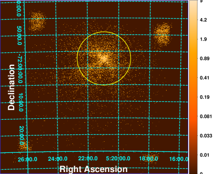
Figure 1: The image of LMC X-2 as observed by SXT in June 2016. The spectra and lightcurves have been extracted from a circular region of 8 arcmin as shown in the figure. The four spots seen at the corners of the image are calibration sources ($Fe^{55}$).

We used XSELECT version 2.4d to extract the image, lightcurves and spectrum from the SXT level2 event files provided by the instrument team. We used a circular region of 8 arcmin centered at the source position to extract the source spectrum and lightcurves. In Figure 1, we show the SXT image of the LMC X-2 for the Orbit number 3977. We created the instrument ARF using the tool sxtmkarf provided by instrument team , which also takes care of the off-pointing correction. We utilized the latest version of the software “LaxpcSoft” provided by the LAXPC team to analyze the LAXPC data and followed the procedure described there (see also Agrawal et al. 2018; Sreehari et al. 2019).

3 Data Analysis

3.1 Lightcurve and Z-track

We used the top layer LAXPC10 event data to construct the lightcurve. Since above 20 keV the intensity is dominated by the contribution from the background, we created the lightcurve in the energy band of $3.0-20.0$ keV. In Figure 2, we show the background subtracted binned lightcurve in the energy range of $3.0-20.0$ keV. The binsize used here is 256 seconds. The source exhibited a flare during our observations. The background subtracted lightcurve created using SXT data is shown in Figure 3.

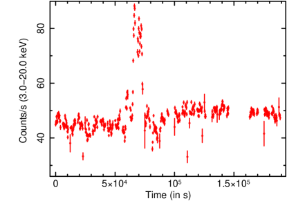
Figure 2: The background subtracted lightcurve of LMC X-2 in the energy range $3.0-20.0$ keV. The lightcurve is created using the LAXPC10 data. The time binsize used for the lightcurve is 256 s.

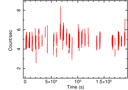
Figure 3: The background subtracted SXT lightcurve of LMC X-2 in the energy range $0.3-8.0$ keV. The time binsize used for the lightcurve is 64 s.

Hardness Intensity Diagram (HID) was created using the background subtracted lightcurves. We defined the overall colours as the ratio of count rates in the energy bands $6.5-18.5$ keV and $3.0-6.5$ keV, whereas intensity was defined as the total count rates in the $3.0-18.5$ keV energy band. We plotted the overall colours against the source intensity to construct the HID. The HID is shown in Figure 4. We used a binsize of 1024 s to create the HID. The large time binsize has been used here to separate the three branches of the Z-pattern. All the three branches of the Z-track can be identified clearly in the HID (Figure 4). The HID shows remarkable similarity with that obtained using the RXTE data (Smale et al., 2003; Agrawal and Misra, 2009).

In order to study the evolution of the broadband spectral and temporal behaviour along the complete Z-track, we divided this track into 7 segments. We divided the horizontal branch (HB) into two sections ‘HB1’ and ‘HB2’. The normal branch (NB) was also divided into two sections namely ‘NB1’, ‘NB2’. The points close to the lower-most NB and the bottom part of the FB are part of the NB-FB vertex (NBV). The rest of the FB was divided into two sections ‘FB1’ and ‘FB2’.

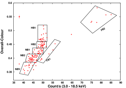
Figure 4: Hardness Intensity Diagram (HID) of LMC X-2 created using the LAXPC10 data. To create the HID, we have used 1024 s binsize. Different sections of the HID have been marked. A typical error bar on the data points is shown in the top-left corner. See text for details.

3.2 Spectral Analysis

We used the LAXPC10 top layer data to create the source and background spectra for different sections of the HID. The latest SXT and LAXPC response matrix files provided by the instrument team were used for the spectral analysis. The sky background spectrum provided by the SXT team was used for the background subtraction. We used combined SXT ($0.5-5.5$ keV) and LAXPC10 ($3.0-20.0$ keV) data for spectral analysis. We restricted our analysis to these energy ranges because there is not enough source flux above 5.5 keV for the SXT and above 20 keV for the LAXPC. The combined spectra in the energy range $0.5-20$ keV were fitted with the XSPEC version 12.9.1. We grouped the SXT data to give a minimum of 25 counts/bin. All the errors were computed using $\Delta\chi^{2}=1.0$ (68% confidence level). We added 1% systematics during fitting to account for the uncertainty in the response matrix.

According to the Dickey and Lockman survey, the galactic $N_{H}$ in the direction of LMC X-2 is 0.063 $\times$ 10²² $cm^{-2}$ (Dickey and Lockman, 1990). However, $N_{H}$ calculated using the more recent surveys like Leiden/Argentine/Bonn (LAB) (Kalberla et al., 2005) and HI4PI (Bailin et al., 2016) is 0.15 $\times$ 10²² $cm^{-2}$. To calculate the $N_{H}$, we used the nH calculator tool provided by HEASARC, NASA. We used the multiplicative model Tbabs of XSPEC to account for the galactic absorption.

First, we fitted the spectra with a simple cutoffpl+bbodyrad model. This model has been used to describe the spectra of Z-sources (Birmingham model; see Jackson et al. 2009; Balucinska-Church et al. 2010). We found that for all parts of the Z-track photon index of the cutoff powerlaw was $<$ 1. Hence cutoff-powerlaw is not consistent with the Comptonization model. We refer to this model as Model 1. We tried using other complex Comptonization models such as nthComp. The nthComp model has provision to select the blackbody or disc blackbody as the input seed photon spectrum (Zdziarski et al., 1996). Yet, another Comptonization model such as compTT which has been used previously to model the spectrum of this source (Lavagetto et al., 2008; Agrawal and Misra, 2009) assumes a Wien spectrum for the seed photons (Titarchuk, 1994). The model provided statistically good fit to the spectra of all the sections of the Z-track. We refer to this model as Model 2. We also tried a combination of disc blackbody (diskbb) and nthComp, as well as a combination of blackbody (bbody) and nthComp model. We noticed that addition of a blackbody or a diskbb component to the nthComp did not improve the fit. This suggests that, probably the disc is obscured by a Comptonized corona. The seed photons for the Comptonization may come from the obscured inner accretion disc or from the surface of the central source. Here, we assumed that the seed photons comes from the accretion disc. However, it is possible that the blackbody emission from the surface of the neutron star may also supply the seed photons for the Comptonization.

Figure 5: The residual in unit of sigma for diskbb+bbodyrad (MCD+BB) model (top panel) and nthComp model (bottom panel). From figure, it is clear that the nthComp model provides a better fit compared to the diskbb+bbodyrad model.

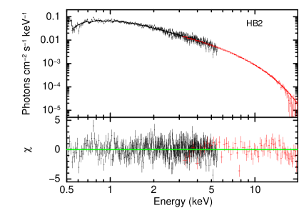
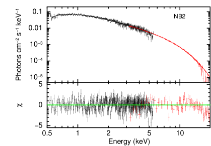
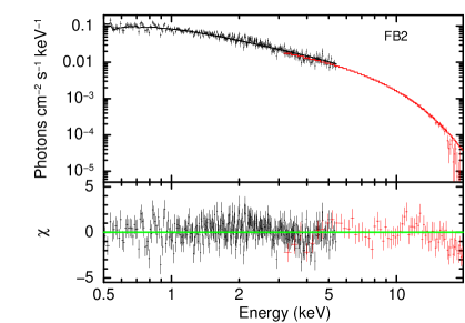
Figure 6: The unfolded spectra at different parts (HB2, NB2, FB2) of the Z-track along with the residual (bottom panels) in the units of sigma.

We also fitted the data with diskbb+bbodyrad model, which has been previously used to model the spectra of this source (Lavagetto et al., 2008) and the other LMXBs (Mitsuda et al., 1984). The above combination provided a poor fit compared to the nthComp model for the HB and NB sections (see Table 2 and Table 3). However, diskbb+bbodyrad and nthComp model gives similar reduced $\chi^{2}$ ($\chi^{2}/dof$) in the FB. We refer to this model as Model 3. In Figure 5, we show the residual resulted by fitting the spectra of the section HB2 with Model 2 and Model 3. From the residual, it is clear that Model 2 (bottom panel of Figure 5) is better compared to Model 3 (top panel of Figure 5). While fitting the spectra with these models, we did not find any residual around $\sim$ $5-7$ keV range, suggesting that the iron line (Fe-K) feature is absent in this source during our observations.

Figure 7: The evolution of the best fit spectral parameters of Model 2 along the Z-track. $y-par$ (Comptonization parameter) and $\tau$ (optical depth) are derived parameters (see text for details).

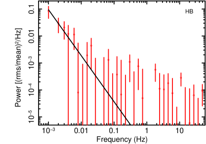
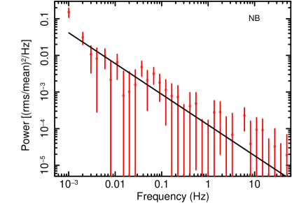
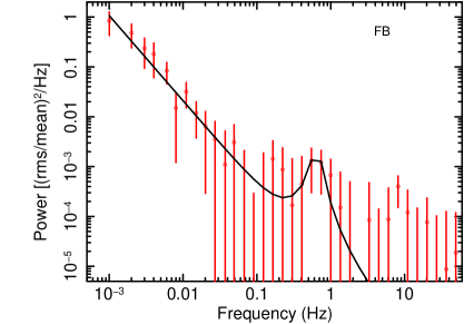
Figure 8: Power density spectra (PDS) for different branches (HB, NB, FB) of the Z-track along with the best fit Model. Marginal detection of QPO-like feature is seen in FB. See, text for details.

3.3 Timing Analysis

We used the LAXPC lightcurves in the energy range $3.0-20.0$ keV to create the PDS. The lightcurves with binsize 4 ms were divided into intervals of 262144 bins, which allowed to study the nature of timing variabilities in the range of $0.001-125.0$ Hz. PDS were created for each interval and those belonging to the same section of the HID are averaged. We rebinned the PDS in the frequency space by a factor of 1.3. The binned PDS were normalized to the fractional rms spectra (in units of $(rms/mean)^{2}Hz^{-1}$) and an appropriate Poisson noise was subtracted (Zhang et al., 1995; Agrawal et al., 2018). To get a better statistics, we merged the PDS belonging to the same branch. While averaging the PDS for the NB branch, we assigned NBV data points as a part of the NB. PDS of all these three branches can be fitted with a simple power-law ($A\nu^{-\alpha}$). While fitting the PDS of FB with a power-law model, we found a signature of a weak QPO-like feature at $\sim$ $0.6-0.7$ Hz. Fitting this feature with an extra Lorentzian component improved the fit. The reduced $\chi^{2}$ decreased from 16.2/32 to 11.5/30.

Table 1: The best fit spectral parameters for Model 1 (Tbabs*(cutoffpl+bbodyrad)). $\Gamma$ is photon index and $E_{C}$ is cutoff energy. $K$ is the normalization of the cutoff powerlaw at 1 keV and in units of $photons/s/cm^{2}/keV$. $N_{BB}$ is the normalization of the blackbody component and $kT_{BB}$ is its temperature. $N_{H}$ is in units of $10^{22}$ cm^-2.

Parameters	HB1	HB2	NB1	NB2	NBV	FB1	FB2
$N_{H}$	0.065(fix)	0.10$\pm$0.01	0.065(fix)	0.065(fix)	0.065(fix)	0.065(fix)	0.065(fix)
$\Gamma$	0.27$\pm$0.06	0.41$\pm$0.06	0.30$\pm$0.06	0.21$\pm$0.05	0.15$\pm$0.07	-0.16$\pm$0.09	-0.26$\pm$0.05
$E_{C}$ (keV)	2.94$\pm$0.08	2.97$\pm$0.08	2.75$\pm$0.06	2.54$\pm$0.05	2.38$\pm$0.06	2.20$\pm$0.06	2.58$\pm$0.05
$K$ ($\times 10^{-2})$	4.85$\pm$0.4	6.28$\pm$0.5	5.86$\pm$0.3	5.45$\pm$0.2	6.76$\pm$0.5	465.6$\pm$0.4	458$\pm$0.3
$kT_{BB}$ (keV)	0.42$\pm$0.01	0.37$\pm$0.01	0.39$\pm$0.01	0.39$\pm$0.06	0.31$\pm$0.02	0.33$\pm$0.01	0.36$\pm$0.01
$N_{BB}$	350.0$\pm$32	515.0$\pm$50.5	390.1$\pm$37.5	445.2$\pm$32.1	1172.5$\pm$240.7	856.4$\pm$92.5	893.8$\pm$65.6
$\chi^{2}/dof$	422/327	667/488	605/378	675/491	216/168	324/299	526/368

Table 2: The best fit spectral parameters for Model 2 (Tbabs*nthComp). $kT_{e}$ and $kT_{s}$ are the electron temperature and seed photon temperature respectively. $\Gamma_{C}$ and $N_{Comp}$ are photon index and the normalization of nthComp component respectively. $\tau$ is the optical depth and $y$-par is the Comptonization parameter. $F_{Comp}$ is the $0.1-50$ keV unabsorbed Comptonization flux in units of ergs/s/cm². $N_{H}$ is the neutral hydrogen column density in untis of 10²² cm^-2. $L_{X}$ is $0.1-50$ keV unabsorbed luminosity in units of ergs/s.

Parameters	HB1	HB2	NB1	NB2	NBV	FB1	FB2
$N_{H}$	0.17$\pm$0.02	0.22$\pm$0.02	0.16$\pm$0.02	0.16$\pm$0.01	0.08${}^{+0.06}_{-0.03}$	0.13$\pm$0.3	0.09$\pm$0.01
$kT_{e}$ (keV)	2.14$\pm$0.02	2.09$\pm$0.02	2.01$\pm$0.02	1.90$\pm$0.01	1.74$\pm$0.02	1.75$\pm$0.02	2.02$\pm$0.02
$\Gamma_{C}$	1.85$\pm$0.01	1.87$\pm$0.01	1.87$\pm$0.01	1.87$\pm$0.02	1.77$\pm$0.02	1.71$\pm$0.01	1.61$\pm$0.01
$kT_{s}$ (keV)	0.38$\pm$0.05	0.27${}^{+0.05}_{-0.11}$	0.39$\pm$0.05	0.37$\pm$0.03	0.38$\pm$0.1	0.23${}^{+0.09}_{-0.07}$	0.32$\pm$0.06
$N_{Comp}(\times 10^{-2})$	9.81$\pm$0.5	11.05${}^{+1.3}_{-0.6}$	10.5$\pm$0.3	9.87$\pm$0.3	9.27${}^{+2.1}_{-0.9}$	9.75$\pm$0.6	10.5$\pm$0.6
$F_{comp}$ $(\times 10^{-10}$)	3.89$\pm$0.09	3.98$\pm$0.09	3.80$\pm$0.17	3.63$\pm$0.08	3.46$\pm$0.08	3.89$\pm$0.09	6.02$\pm$0.14
$R_{W}$ (km)	102$\pm$26.5	206.5$\pm$110.4	97.2$\pm$24.3	149.5$\pm$25.5	89.5$\pm$36.5	253.5$\pm$110.5	150.2$\pm$55.4
$\tau$	13.35$\pm$0.16	13.31$\pm$0.15	13.65$\pm$0.3	14.05$\pm$0.31	15.97$\pm$0.41	16.77$\pm$0.24	17.15$\pm$0.28
$y-par$	2.98$\pm$0.06	2.91$\pm$0.06	2.91$\pm$0.12	2.92$\pm$0.13	3.47$\pm$0.15	3.85$\pm$0.11	4.62$\pm$0.14
$L_{X}$ $(\times 10^{38})$	1.15$\pm$0.02	1.18$\pm$0.03	1.13$\pm$0.05	1.08$\pm$ 0.02	1.03$\pm$0.02	1.15$\pm$0.03	1.79$\pm$0.04
$\chi^{2}/dof$	415/327	663/489	604/378	675/491	197/168	309/299	484/368

Table 3: The best fit spectral parameters for Model 3 (Tbabs*(diskbb + bbodyrad). $kT_{bb}$ is the blackbody temperature and $kT_{in}$ is the inner disc temperature. $N_{bb}$ and $N_{dbb}$ are the normalization of the bbodyrad and diskbb components respectively. $N_{H}$ is in units of 10²² cm^-2.

Parameters	HB1	HB2	NB1	NB2	NBV	FB1	FB2
$N_{H}$	0.09$\pm$0.01	0.09$\pm$0.01	0.10$\pm$0.006	0.063(fixed)	0.07$\pm$0.01	0.063(fixed)	0.063(fix)
$kT_{in}$ (keV)	0.97$\pm$0.02	0.88$\pm$0.01	0.93$\pm$0.02	0.84$\pm$0.02	0.87$\pm$0.02	0.81$\pm$0.02	0.92$\pm$0.01
$N_{dbb}$	19.42$\pm$1.92	29.71$\pm$1.85	22.91$\pm$2.07	32.29$\pm$2.04	28.48$\pm$3.36	35.27$\pm$4.12	27.35$\pm$1.65
$kT_{bb}$ (keV)	1.80$\pm$0.02	1.72$\pm$0.01	1.71$\pm$0.01	1.60$\pm$0.01	1.54$\pm$0.01	1.51$\pm$0.01	1.79$\pm$0.01
$N_{bb}$	2.21$\pm$0.11	2.70$\pm$0.10	2.71$\pm$0.13	3.32$\pm$0.13	4.35$\pm$0.24	4.87$\pm$0.26	4.56$\pm$0.15
$R_{dbb}\sqrt{\cos\theta}$ (km)	22.03$\pm$1.08	27.25$\pm$0.85	23.95$\pm$1.08	28.42$\pm$0.89	26.68$\pm$1.58	29.70$\pm$1.72	26.15$\pm$0.78
$R_{bb}$ (km)	7.43$\pm$0.18	8.21$\pm$0.15	8.23$\pm$0.19	9.09$\pm$0.18	10.42$\pm$0.28	11.03$\pm$0.29	10.67$\pm$0.17
$\chi^{2}$/dof	440/327	759/489	651/378	705/491	211/168	307/300	481/369

Table 4: The best fit parameters obtained by fitting the PDS of different branches of the Z-track. $\alpha$ is the index and $A$ is the normalization of the power-law component. Pow-rms is the total rms of the power-law component in the frequency range $0.001-50$ Hz and QPO-rms is the rms of the QPO feature in the frequency range $0.001-50$ Hz.

Parameters	HB	NB	FB
$\alpha$	1.70$\pm$0.22	0.83$\pm$0.12	1.71$\pm$0.11
$A$($\times 10^{-5}$)	0.078$\pm$0.03	13.4$\pm$2.5	0.87$\pm$0.3
Pow-rms (%)	1.21$\pm$0.82	3.61$\pm$1.62	3.97$\pm$1.58
$\nu_{c}$ (Hz)			0.65$\pm$0.07
$FWHM$ (Hz)			0.2 (fixed)
LN ($\times$ 10-3)			2.48$\pm$0.84
QPO-rms (%)			2.71$\pm$0.52
F-test			5.8 $\times$ 10-3
$\chi^{2}$/dof	27.1/32	26.2/32	11.5/30

4 Results

4.1 Spectral Behaviour

The broadband spectra ($0.5-20.0$ keV) along the Z-track can be fitted with an absorbed Comptonization model (Model 2). We also tried the combination of emission from the multicolour disc (described by diskbb in XSPEC) and blackbody component (Model 3). We found that Model 3 is not satisfactory for describing the spectra of the HB and the NB (see Table 3). The spectral parameters and reduced $\chi^{2}$ of Model 2 and Model 3 are given in Table 2 and Table 3 respectively. Model 3 gave the inner disc temperature in the range of $\sim$ $0.8-1.0$ keV and black body temperature in the range of $1.5-1.8$ keV. In Figure 6, we show the spectra of the HB2, NB2 and FB2 fitted with Model 2. The $N_{H}$ values derived using Model 2 lie in the range of $(0.1-0.2)$ $\times$ $10^{22}cm^{-2}$. The derived $N_{H}$ values in the direction of LMC X-2 are close to the results of recent surveys (Kalberla et al., 2005; Bailin et al., 2016). Moreover, systematics in the data and model can also affect the best-fit values of $N_{H}$.

Fitting the spectra with Model 2 gave the electron temperature in the range of $1.7-2.1$ keV (see Table 2). The electron temperature decreased as the source moved from the HB to the NB and then again increased as it moved up along the FB. The photon index of the Comptonized emission was around $\sim$ 1.85 from the top-left HB to the lower NB. Then as the source moved down the NB-FB vertex (NBV) and then up in the FB the photon index decreased or the source spectrum became harder. We also computed the optical depth by formula given in Zdziarski et al. (1996) and the Comptonization parameter using a relation $y=\frac{4kT_{e}}{m_{e}c^{2}}max(\tau,\tau^{2})$. The optical depth did not show significant change from HB1 to NB2 and remained in the range of   $13.2-14.3$. As the source moved to the vertex (NBV), the optical depth increased from 14.05$\pm$0.31 to 15.97$\pm$0.41 and continued to increase along the FB. The Comptonization parameter $y$ decreased from $\sim$ 2.98 to to $\sim$ 2.92 as the source moved down the HB and then remained constant in the NB (NB1 and NB2). The $y$ parameter increased from 3.47$\pm$0.15 to 4.62$\pm$0.14 with the movement of the source from the vertex (NBV) to the FB2. Since the distance ($\sim$ 50 kpc) to the source is known with a better accuracy (Freedman et al., 2001), the uncertainty in the intrinsic luminosity of the source is also much less compared to other Z-sources. The luminosity of the source showed a systematic decrease as the source moved from the upper NB to the vertex (NBV), and as the source further moved up the FB the luminosity increased. The luminosity varied in the range $(1.03-1.79)$ $\times 10^{38}$ ergs/s. We show the evolution of the best fit spectral parameters of Model 2 in Figure 7.

We also computed the the radius of the seed photon emitting region using the formula (see in ’t Zand et al. 1999),

$$R_{W}=3\times 10^{4}D\frac{\sqrt{\frac{f_{bol}}{1+y}}}{kT_{s}^{2}}.$$ (1)

The Wein radius $R_{W}$ was found to be in the range of $70-310$ km and did not show any clear correlation with the position on the Z-track (see Table 2). Here, $D$ is the distance to the source in kpc, $y$ is the Comptonization parameter and $f_{bol}$ is the bolometric ($0.1-50$ keV) flux of the Comptonized component.

We also derive the inner disc radius and the blackbody radius using the parameters of Model 3. The inner disc radius $R_{dbb}\sqrt{\cos\theta}$ is given by $\sqrt{N_{dbb}}D_{10}$, where $\theta$ is the inclination angle and $D_{10}$ is the distance to the source in the unit of 10 kpc. Similarly, the radius of blackbody emitting region is given by $\sqrt{N_{bb}}D_{10}$. The inner disc radius is found to be in the range of $20-30$ km and the blackbody radius varies in the range of $7-11$ km.

4.2 Power-spectral Properties

We detected very low-frequency noise (VLFN) in all the three branches (HB, NB and FB). For the NB, we found index $\alpha$ = 0.83$\pm$0.11 and integrated rms ($0.001-50$ Hz) = 3.61$\pm$1.62%. The VLFN in the HB has integrated rms = 1.21$\pm$0.82% and that in the FB has integrated rms = 3.97$\pm$1.58%. We found a marginal evidence of QPO at 0.65$\pm$0.07 Hz in the FB with significance $\sim$ 2.8 $\sigma$ and integrated rms ($0.001-50$ Hz) = 2.71$\pm$0.52%. The best fit PDS model parameters for HB, NB and FB are presented in Table 4. Figure 8 shows the PDS for these three branches along with the best fit model.

5 Discussion

The bright low-mass X-ray binary LMC X-2 traced a complete Z-track during the $\sim$ 140 ks LAXPC observations. We also note that the range of the overall color values ($0.3-0.6)$ during our observations is similar to that observed during the RXTE observations (Smale et al., 2003; Agrawal and Misra, 2009). The track in the HID is almost identical during the RXTE and the present AstroSat observations. We also note that the source spent $\sim$ 12 ks or 8% time in the flaring state. Using these observations, we studied the evolution of the broadband ($0.5-20$ keV) spectral parameters along the complete Z-track by combining the SXT and LAXPC data, which is a first such study. Previously, spectral evolution of the source has been investigated along the Z-track using the data from the RXTE-PCA in the energy range of $3.0-20.0$ keV (Agrawal and Misra, 2009).

Here, we have shown that the $0.5-20.0$ keV spectra of the source can be described by a simple absorbed Comptonization model (Model 2). We find that the Comptonizing region is cool and optically thick with the electron temperature in the range of $\sim$ $1.7-2.1$ keV and the optical depth in the range of $\sim$ $13.2-17.5$. The RXTE-PCA spectra in the $3.0-20.0$ keV energy band, fitted with compTT model provided a similar optical depth ($\tau\sim 13.0-18.0$) but a slightly higher electron temperature ($kT_{e}\sim 1.95-2.7$ keV) (Agrawal and Misra, 2009).

Most importantly, we do not require an extra disc emission component or a blackbody component to fit the spectra in the $0.5-20.0$ keV range unlike Suzaku observations (Agrawal and Misra, 2009). It is worth mentioning that the $0.3-10.0$ keV XMM-Newton spectrum of the source was also modeled using a pure Comptonized emission (Lavagetto et al., 2008). The possible explanation for the absence of the soft component is that the temperature of the soft component may be well below the lower energy bound of the instrument, considered while fitting. The seed photon temperature $kT_{s}$ in our case is $\sim$ $0.2-0.4$ keV. However, a significantly lower value of $kT_{s}$ ($\sim$ 40 eV) has been reported by Lavagetto et al. (2008) using the XMM-Newton observation. They also calculated the radius of seed photons emitting region and it was found to be very high ($R_{W}\sim 10^{4}$ km) and which lead to conclusion that Comptonization model is not physically acceptable. In our case, the radius of seed photon emitting region is $70-310$ km and hence the Comptonization model (nthComp) is an appropriate to represent the spectra of the source along the Z-track.

We have studied the evolution of the spectral parameters along the Z-tarck. Though variations in these parameters are subtle, they provide an important probe to understand the movement of the source along the Z-pattern. Our findings suggest that the optical depth of the corona increases as the source moves from the NB-FB vertex (NBV) to the upper FB. We also note that the Compton $y$ parameter also increases along the FB. This trend is also seen in other Z-sources (GX 349+2: Agrawal and Sreekumar 2003, GX 17+2: Agrawal et al. 2020) and in the previous observations of LMC X-2 (Agrawal and Misra, 2009). The observed variations in the spectral parameters ($\tau$ and $y$) suggest that most probably at the vertex of the NB and the FB, the accretion rate crosses the Eddington limit and a strong radiation pressure drives a fraction of the disc material into a hot central corona. The above scenario has been discussed by Agrawal and Sreekumar (2003); Agrawal et al. (2020) to explain the increase of the optical depth along the FB in the Z-sources GX 349+2 and GX 17+2. Hence, the motion from the vertex to the upper FB can be understood in terms of increasing accretion rate scenario.

It has been observed that in some of the Z-sources the optical depth of the Comptonized component generally decreases as the source moves from the HB to the lower NB (GX 17+2: Di Salvo et al. 2000; Agrawal et al. 2020, GX 349+2: Agrawal and Sreekumar 2003, GX340+0: Iaria et al. 2006, Cyg X-2: Di Salvo et al. 2002) and the electron temperature either remains constant (Agrawal et al., 2020; Di Salvo et al., 2000) or increases (Di Salvo et al., 2002; Agrawal and Sreekumar, 2003; Iaria et al., 2006). In the present case, the electron temperature of the Comptonizing region decreases as the source moves from HB to the vertex of the NB and FB. However, the optical depth remains nearly constant upto the middle of NB (NB2). The source exhibited a similar behaviour during the RXTE observations (Agrawal and Misra, 2009). The decrease in the $kT_{e}$ can be explained in terms of cooling of the corona due to increase in the seed photon supply. However, it is also possible that a part of the coronal material cools down and settles in the disc causing the optical depth to decrease and the temperature of the remaining material in the corona will either not change or will increase. The above scenario can explain the spectral behaviour of other Z-sources.

We have derived PDS for the three branches (HB, NB and FB). In all three branches, PDS has the VLFN component. Smale et al. (2003) found VLFN component with $\alpha$ $\sim$ 0.60 in the HB, $\alpha$ $\sim$ 0.90 in the NB and $\alpha\sim$ 1.33 in the FB. In our case, the VLFN in the HB and FB is steeper compared to the previous results (Smale et al., 2003). However, the value of VLFN index in the NB is close to that obtained by Smale et al. (2003). We also detect a weak ($\sim$ $2.8~{}\sigma)$ QPO at $\sim$ 0.65 Hz in the FB. The rms amplitude of the QPO is $\sim$ 2.7%.

data availability

Data underlying this article are available at AstroSat-ISSDC website (http://astrobrowse.issdc.gov.in/astro_archive/archive).

References

- Agrawal et al. (2020) Agrawal V. K., Nandi Anuj, Ramadevi M. C., 2020, Ap&SS, 365, 41
- Agrawal et al. (2018) Agrawal V.K., Nandi Anuj, Girish V., Ramadevi M.C., 2018, MNRAS, 477, 5437
- Agrawal and Misra (2009) Agrawal V.K., Misra R., 2009, MNRAS, 398, 1352
- Agrawal and Sreekumar (2003) Agrawal V.K., Sreekumar P., 2003, MNRAS, 346, 933
- Bailin et al. (2016) Bailin J., Calabretta M.R., Dedes L., Ford H.A., Gibson B.K., Haud U., Janowiecki S., Kalberla P.M.W. et al., 2016, A&A, 594, A116
- Balucinska-Church et al. (2010) Balucinska-Church M., Gibbec A., Jackson N.K., Church M.J., 2010, A&A,512, A9
- Bhulla et al. (2019) Bhulla Y., Misra R., Yadav J.S. et al.,2019, RAA, 19, 114
- Bonnet-Bidaud et al. (1989) Bonnet-Bidaud J.M., Motch C, Beuermann K., Pakull M., Parmar A.N., van der Klis M., 1989, A&A, 213, 97
- Cackett et al. (2010) Cackett E.M., Miller J. M., Ballantyne D. R., Barret D., Bhattacharyya S., Boutelier M., Miller M.C., Strohmayer T. E., 2010, ApJ, 720, 205
- Church et al. (2012) Church M.J., Gibiec A., Balucinska-Church M., Jackson N.K., 2012, A&A, 546, A35
- Dickey and Lockman (1990) Dickey J.M., Lockman F.J., ARA&A, 1990, 28, 215
- Di Salvo et al. (2002) Di Salvo T. et al., 2002, A&A, 386, 535
- Di Salvo et al. (2001) Di Salvo T., et al., 2001,ApJ, 554, 49
- Di Salvo et al. (2000) Di Salvo T., Stella L., Robba N.R., van der Klis M., Burderi L., Israel G.L, Homan J., Compana S. et al., 2000, ApJ, 544, L119
- Done, Zycki and Smith (2002) Done C., Zycki P.T. and Smith D.A, 2002, MNRAS, 331, 453
- Farinelli et al. (2009) Farinelli R., Paizis A., Landi R., and Titarchuk L.,2009, A&A, 498, 509
- Freedman et al. (2001) Freedman W.L., Madore B.F., Gibson B.K. et al., 2001, ApJ, 553, 47
- Hasinger and van der Klis (1989) Hasinger G., van der Klis M., 1989, A&A, 225, 79
- in ’t Zand et al. (1999) in ’t Zand, J.J.M., Verbunt F., Strohmayer T.E., Bazzano A., Cocchi M., Heise J., van Kerkwijk M.H., Muller J.M., et al., 1999, A&A, 345, 100
- Iaria et al. (2006) Iaria R., Lavagetto G., Di Salvo T., D’ Ai A., Burderi L., Stella L., Robba N. R., 2006, Chin. J. Astron. Astrophys., 6, 257
- Jackson et al. (2009) Jackson N.K., Church M.J., Balucinska-Church M., 2009, A&A, 494,1059
- Johnston et al. (1979) Johnston M.D., Bradt H.V., Doxsey R.E., 1979, ApJ, 233 514
- Kalberla et al. (2005) Kalberla P.M.W., Burton W.B., Hartmann D., Arnal E.M., Bajaja E., Morras R., Poppel W.G.L, 2005, A&A 440, 775
- Lavagetto et al. (2008) Lavagetto G., Iaria R., D’Ai A., Di Salvo T., Robba N. R., 2008,A&A, 478,181
- Lin et al. (2012) Lin D., Remillard R.A., Homan J., Barret D., 2012, ApJ, 756, 34
- Markert and Clark (1975) Markert T.H., Clark G.W., 1975, ApJ, 196, L55
- Pakull (1978) Pakull M., 1978, IAU Circular, 3313
- Singh et al. (2016) Singh, K.P, Stewart G.C., Chandra S., Mukerjee K., Kotak S., Beardmore, A.P., Chitnis V., Dewangan G.C., et al., 2016, SPIE, 99051E, 10
- Smale and Kuulkers (2000) Smale A.P., Kuulkers E., 2000, ApJ 528, 702
- Smale et al. (2003) Smale A.P., Homan J., Kuulkers E., 2003, ApJ, 590, 1035
- Mitsuda et al. (1984) Mitsuda K., et al., 1984, PASJ, 36, 741
- Titarchuk (1994) Titarchuk L., 1994, ApJ, 434,570
- Vadawale et al. (2016) Vadawale, S.V., Rao A.R., Bhattacharya D., Bhalerao Varun B., Dewangan G.C., Vibhute A.M., Mithun N.P.S., Chattopadhyay T., et al, 2016, SPIE, 9905, 11
- van der Klis (2000) van der Klis M., 2000, ARA&A, 38, 717
- Yadav et al. (2016) Yadav J.S., Agrawal P.C., Antia H.M., Chauhan Jai Verdhan, Dedhia Dhiraj, Katoch Tilak, Madhwani P., Manchanda R.K, et al., 2016, SPIE, 9905, 15
- Zdziarski et al. (1996) Zdziarski A. A., Johnson W.N., Magdziarz P., 1996, MNRAS, 283, 193
- Zhang et al. (1995) Zhang W., Jahoda K., Swank J.H., Morgan E.H. and Giles A.B., 1995, ApJ, 449, 930