holographic superconductor in AdS3 spacetime

Abstract

We do more discussions of holographic s-wave superconductors in the background of AdS3 spacetime. We analytically compute the holographic superconductor model with the motion equation has two different characteristic root on the framework of Maxwell electrodynamics field. We study superconductor models on the framework of Born-Infeld electrodynamics field and on the framework of the Stückelberg form in the background of AdS3 spacetime.

1 introduction

The AdS/CFT correspondence[1] indicates that a weak coupling gravity theory in (d+1)-dimensional AdS spacetime can be described by a strong coupling conformal field theory on the d-dimensional boundary. This means that the AdS/CFT correspondence could help us understand more deeply about the strong coupled gauge theories[2][3][4] and offer us a new means of studying the strongly interacting condensed matter systems in which the perturbation methods are no longer valid[5][6][7]. Recently, this holographic method is also expected to give us some insights into the nature of the pairing mechanism in the high temperature superconductors which is beyond the scope of current theories of superconductivity. The earliest models for holographic superconductors in the AdS black hole spacetime are proposed in [8][9][10][11], where the black hole admits scalar hair at the temperature $T$ smaller than a critical temperature $T_{c}$, but does not possess scalar hair at higher temperatures. According to the AdS/CFT correspondence, the appearance of a hairy AdS black hole at low temperature implies the formation of the scalar condensation in the boundary CFT, which makes the expectation value of charged operators undergo the U(1) symmetry breaking and results in the occurrence of the phase transition. Due to its potential applications to the condensed matter physics, the properties of the holographic superconductors in the various theories of gravity have been investigated extensively[12][13][14][15][16] [17][18][19][20][21][22][23][24] in recent years.

AdS3 spacetime as an interesting gravity model has been studied in many works since it proposed in [25]. Some holographic properties and superconductor phase transitions in AdS3 spacetime background have been discussed in [26][27][28][29]. But up to now, researches of holographic superconductor on AdS3 spacetime are obviously less than on other spacetimes, and researches are limited to the second phase transition based on the framework of Maxwell electrodynamics. In this paper, we will do more discussion on holographic superconductors on the framework of Maxwell electrodynamics and on the framework of Born-Infeld electrodynamics, and give the properties of holographic superconductors on the framework of the Stückelberg mechanism form in AdS3 spacetime.

On the framework of Maxwell electrodynamics, reference [27] and [29] have respectively given the numerical solution and analytical solution in the model of one-dimensional holographic superconductor when the mass of scalar field is equal to Breitenlohner-Freedman bound, i.e. $m^{2}=-1$, the scalar field equation has two same characteristic root $\Delta_{\pm}=1$ and its asymptotically behaves are $\psi\sim z\ln z$ and $\psi\sim z$. Furthermore we will discuss the general situation that the equation has two different characteristic root $\Delta_{\pm}$, and the scalar field asymptotically behaves are $\psi\sim z^{\Delta_{\pm}}$.

It is well known that the properties of holographic superconductors depend on behaviors of the electromagnetic field coupled with the scalar filed in the system. critical temperature and the critical exponent near the point

Different from Maxiwell electrodynamics, Born-Infeld electrodynamics[30] is one of the important nonlinear electromagnetic theories, which was introduced by Born and Infeld in 1934 to deal with the infinite self energies for charged point particles arising in Maxwell theory. As a candidate of many improved models of Maxwell theory, it is the only electric-magnetic duality invariance theory[31] which has been researched extensively[32][33][34]. In particular, the effects of Born-Infeld electrodynamics on the holographic superconductors has been studied numerically in [35][36][37][38][39][40][41][42][43][44][45][46]. In this paper, we are going to investigate how the Born-Infeld electrodynamics affect the holographic superconductors phase transition in AdS3 spacetime background.

We will also discuss a generalization of the basic holographic superconductor model in which the spontaneous breaking of a global U(1) symmetry occurs via the Stückelberg mechanism[20][47][48] in AdS3 spacetime background. The generalized Stückelberg mechanism of symmetry breaking can describe a wider class of phase transitions including the first order phase transition and the second order phase transition. We are going to investigate how the Stückelberg form affect the critical temperature, the order of phase transitions and the critical exponent near the phase transition point in AdS3 spacetime background.

This paper is organized as follows. First we discuss the holographic superconductor model with two different characteristic root on the frame of Maxwell electrodynamics in AdS3 spacetime in section 2. Then an analytically study of the scalar condensation and the phase transitions of holographic superconductor on the frame of Born-Infeld electrodynamics in AdS3 spacetime is given. In Sect.4, we calculate a general class of the holographic superconductor model on the frame of the Stückelberg form in AdS3 spacetime. The last section is the conclusion which contains our main results.

2 AdS3 superconductors on Maxwell electrodynamics

On the framework of Maxwell electrodynamics, reference [27] and [29] have respectively given the numerical solution and analytical solution with the motion equation has two same characteristic root in the model of one-dimensional holographic superconductor. However, in this section, we will give more discussion on AdS3 holographic superconductors analytically that the motion equation has two different characteristic root on the framework of Maxwell electrodynamics.

The line element of the AdS3 black hole can be written as

$$ds^{2}=-\frac{1}{z^{2}}f(z)dt^{2}+\frac{dz^{2}}{f(z)}+dx^{2},$$ (1)

where $f(z)=-M+r_{+}^{2}/z^{2}l^{2}$. Its Hawking temperature is

$$T=\frac{r_{+}}{2\pi}.$$ (2)

The action for a Maxwell electromagnetic field coupling with a charged scalar field in AdS3 spacetime reads

$$\mathcal{L}=-\frac{1}{4}F^{\mu\nu}F_{\mu\nu}-|\nabla_{u}\psi-iA_{\mu}\psi|^{2}-V(|\psi|).$$

The equations of the motions are described by

$$\phi^{\prime\prime}+\frac{1}{z}\phi^{\prime}-\frac{2\psi^{2}}{z^{2}(1-z^{2})}\phi=0,$$ (3)

$$z\psi^{\prime\prime}-\frac{1+z^{2}}{1-z^{2}}\psi^{\prime}+\left[\frac{z\phi^{2}}{r_{+}^{2}(1-z^{2})^{2}}-\frac{m^{2}}{z(1-z^{2})}\right]\psi=0.$$ (4)

Unlike Ref.[29], here we will discuss the situation that the motion equation has two different characteristic root $\Delta_{\pm}$, and at the spatial infinity, the matter fields have the form

$$\psi=\psi^{\pm}z^{\Delta_{\pm}},$$ (5)

$$\phi=\mu\ln z+\rho,$$ (6)

where $\Delta_{\pm}=1\pm\sqrt{1+m^{2}}$. According to the AdS/CFT correspondence, the dual relation of scalar operators $\langle\mathcal{O}_{\Delta_{\pm}}\rangle$ and scalar field $\psi^{\pm}$ is

$$\langle\mathcal{O}_{\Delta_{\pm}}\rangle\sim r_{+}^{\Delta_{\pm}}\psi^{\pm}.$$ (7)

At the critical temperature $T_{c}$, $\psi=0$, so Eq.(3) reduces to

$$\phi^{\prime\prime}+\frac{1}{z}\phi^{\prime}=0.$$ (8)

Let us set $\phi(z)=\lambda r_{+c}\ln z,~{}\lambda=\mu/r_{+c}$ . Near the boundary, we introduce a new function $F(z)$ which satisfies $\psi(z)=z^{\Delta}F(z)\langle\mathcal{O}_{\Delta}\rangle/r_{+}^{\Delta}$, where $F(0)=1$. At $T\rightarrow T_{c}$, the field equation of $\psi$ becomes

$$-F^{\prime\prime}+\frac{1}{z}\left(\frac{1+z^{2}}{1-z^{2}}-2\Delta\right)F^{\prime}+\frac{\Delta^{2}}{1-z^{2}}F=\frac{\lambda^{2}\ln^{2}z}{(1-z^{2})^{2}}F$$ (9)

to be sloved subject to the boundary condition $F^{\prime}(0)=0$.

According to the Sturm-Liouville eigenvalue problem, the minimum eigenvalue $\lambda$ is

$$\lambda^{2}=\frac{\int_{0}^{1}dz~{}z^{-1+2\Delta}[(1-z^{2})F^{\prime}(z)^{2}+\Delta^{2}F(z)^{2}]}{\int_{0}^{1}dz~{}z^{-1+2\Delta}\frac{\ln^{2}z}{1-z^{2}}F(z)^{2}}.$$ (10)

We use $F(z)$ as the following trial function

$$F=F_{\alpha}(z)\equiv 1-\alpha z^{2}.$$ (11)

If $\Delta=1/2$, we have

$$\lambda_{\Delta=1/2}^{2}=\frac{\frac{1}{4}-\frac{\alpha}{6}+\frac{7\alpha^{2}}{12}}{4\alpha-\frac{56\alpha^{2}}{27}+\frac{7}{4}(\alpha-1)^{2}\zeta(3)}.$$ (12)

When $\alpha\approx 0.12$, it has the minimum $\lambda^{2}\approx 0.115$. If $\Delta=3/2$, we have

$$\lambda_{\Delta=3/2}^{2}=\frac{\frac{3}{4}-\frac{9\alpha}{10}+\frac{11\alpha^{2}}{20}}{-2-\frac{2\alpha(-7000+3527\alpha)}{3375}+\frac{7}{4}(\alpha-1)^{2}\zeta(3)}.$$ (13)

When $\alpha\approx 0.60$, it has the minimum $\lambda^{2}\approx 5.586$.

And the critical temperature can be deduced[29]

$$T_{c}=\frac{r_{+c}}{2\pi}=\frac{1}{2\pi}\frac{\mu}{\lambda}.$$ (14)

Away from (but close to) the critical temperature, the field equation (3) of $\phi$ is

$$\phi^{\prime\prime}+\frac{1}{z}\phi^{\prime}-\frac{2\langle\mathcal{O}_{\Delta}\rangle^{2}}{r_{+}^{2\Delta}}\frac{z^{2(\Delta-1)}F^{2}(z)}{1-z^{2}}\phi=0.$$ (15)

Because the parameter $\langle\mathcal{O}_{\Delta}\rangle^{2}/r_{+}^{2\Delta}$ is small, we can expand $\phi(z)$ in the parameter $\langle\mathcal{O}_{\Delta}\rangle^{2}/r_{+}^{2\Delta}$

$$\frac{\phi}{r_{+}}=\lambda\ln z+\frac{\langle\mathcal{O}_{\Delta}\rangle^{2}}{r_{+}^{2\Delta}}\chi(z)+\cdots.$$ (16)

Substituting the above formulation into Eq.(15), the equation of $\phi$ is translated into the equation of $\chi$

$$\chi^{\prime\prime}+\frac{1}{z}\chi^{\prime}=\lambda\frac{z^{2(\Delta-1)}F^{2}(z)}{1-z^{2}}\ln z,$$ (17)

where the boundary condition becomes $\chi(1)=0$.

According to [49][29], its solution can be written as

$$z\chi^{\prime}_{1}(0)=\lambda\mathcal{C},\qquad\mathcal{C}=\int_{0}^{1}dz\frac{z^{2\Delta-1}F^{2}(z)}{1-z^{2}}\ln z,$$ (18)

then we have the expression

$$\frac{\mu}{r_{+}}=\lambda\left(1+\frac{\mathcal{C}\langle\mathcal{O}_{\Delta}\rangle^{2}}{r_{+}^{2\Delta}}+\cdots\right)$$ (19)

and the operation $\langle\mathcal{O}_{\Delta}\rangle$ near the critical temperature

$$\langle\mathcal{O}_{\Delta}\rangle\approx\gamma T_{c}^{\Delta}\left(1-\frac{T}{T_{c}}\right)^{\frac{1}{2}},\qquad\gamma=\frac{(2\pi)^{\Delta}}{\sqrt{\mathcal{C}}}.$$ (20)

3 AdS3 superconduction on Born-Infeld electrodynamics

In this section we will give the holographic superconductor on the frame of Born-Infeld electromagnetic field in AdS3 spacetime.

3.1 superconduction phase in Born-Infeld electrodynamics

We rewriter the three-dimensional AdS metric Eq.(1) in the form[25]

$$ds^{2}=-f(r)dt^{2}+f(r)^{-1}dr^{2}+r^{2}dx^{2}.$$ (21)

The Hawking temperature of black hole is

$$T_{H}=\frac{1}{2\pi}r_{+},$$ (22)

where $r_{+}$ is the event horizon of the black hole.

We consider a Born-Infeld field and a charged complex scalar field coupled via the action

$$S=\int d^{4}x\sqrt{-g}\left(\mathcal{L}_{BI}-\left|\nabla_{\mu}\psi-iqA_{\mu}\psi\right|^{2}-m^{2}\left|\psi\right|^{2}\right)$$ (23)

with

$$\mathcal{L}_{BI}=\frac{1}{b}\left(1-\sqrt{1+\frac{bF}{2}}\right),$$ (24)

where $F\equiv F_{\mu\nu}F^{\mu\nu}$.

Taking the ansatz that $\psi=\psi(r)$ and $A_{\mu}$ has only the time component $A_{t}=\phi$, we can get the equations of motion for the scalar field $\psi$ and gauge field $\phi$ in the form

$$\phi^{\prime\prime}+\frac{1}{r}\phi^{\prime}(1-b\phi^{\prime 2})-\frac{2\psi^{2}}{f}\phi(1-b\phi^{\prime 2})^{\frac{3}{2}}=0,$$ (25)

$$\psi^{\prime\prime}+\left(\frac{f^{\prime}}{f}+\frac{1}{r}\right)\psi^{\prime}+\frac{\phi^{2}}{f^{2}}\psi-\frac{m^{2}}{f}\psi=0.$$ (26)

Near the boundary $r\rightarrow\infty$, the matter fields have the asymptotic behaviors

$$\psi=\frac{\psi^{\pm}}{r^{\triangle_{\pm}}},$$ (27)

$$\phi=-\mu\ln r+\rho,$$ (28)

where $\mu$ and $\rho$ are interpreted as the chemical potential and charge density in the dual field theory respectively. From the dual field theory, the dual relation of scale operate $\mathcal{O}$ and field $\psi_{\pm}$ can be written as

$$\langle\mathcal{O}_{\pm}\rangle\sim\psi_{\pm},$$ (29)

In Figure 1 we present the condensation of the scalar operators $\langle{\cal O}_{+}\rangle$ as a function of temperature with various correction terms $b$. We find that the condensation gap increases with the Born-Infeld scale parameter $b$, which means that the scalar hair is harder to be formed than the usual Maxwell field. This behavior is reminiscent of that seen for the 4-dimension holographic superconductors with Born-Infeld electrodynamics[35], where the higher Born-Infeld corrections make condensation harder.

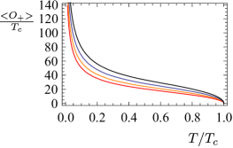
Figure 1: (Color online) The condensate $\langle\mathcal{O}_{i}\rangle$ as a function of temperature $T$ with different $b$. The four lines correspond to increasing $b$, i.e., $0$ (red), $0.01$ (orange), $0.02$ (blue), $0.03$ (black) from bottom to top as $\triangle=1/2$.

3.2 analytical understanding of critical temperature

Here we will apply the Sturm-Liouville method[49] to analytically investigate the properties of holographic superconductor phase transition with Born-Infeld electromagnetic field.

Introducing a new variable $z=r_{+}/r$, we can rewrite Eq.(25) and Eq.(26) into

$$\phi^{\prime}(z)+\frac{bz^{4}\phi^{\prime}(z)^{3}}{r_{+}^{2}}+\frac{2\phi(z)\psi(z)^{2}\left[1-\frac{bz^{4}\phi^{\prime}(z)^{2}}{r_{+}^{2}}\right]^{\frac{3}{2}}}{-z+z^{3}}+z\phi^{\prime\prime}(z)=0,$$ (30)

$$\left[\frac{m^{2}}{z\left(-1+z^{2}\right)}+\frac{z\phi(z)^{2}}{r_{+}^{2}\left(-1+z^{2}\right)^{2}}\right]\psi(z)+\frac{\left(1+z^{2}\right)\psi^{\prime}(z)}{-1+z^{2}}+z\psi^{\prime\prime}(z)=0.$$ (31)

The asymptotic boundary conditions for the scalar potential $\phi(z)$ and the scalar field $\psi(z)$ turn out to be

$$\psi=\psi^{\pm}z^{\triangle_{\pm}},$$ (32)

$$\phi=\mu\ln z+\rho,$$ (33)

and relation Eq.(29) becomes

$$\langle\mathcal{O}_{\Delta_{\pm}}\rangle\sim r_{+}^{\Delta_{\pm}}\psi^{\pm}.$$ (34)

With the above set up in place, we are now in a position to investigate the relation between the critical temperature and the charge density. At the critical temperature $T_{c}$, $\psi=0$, so the Eq.(30) reduces to

$$\phi^{\prime\prime}(z)+\frac{bz^{3}\phi^{\prime}(z)^{3}}{r_{+}^{2}}+\frac{\phi^{\prime}(z)}{z}=0.$$ (35)

Letting $\phi^{\prime}(z)=1/\sqrt{\zeta}$, we have

$$-\frac{1}{2}\zeta^{\prime}(z)+\frac{bz^{3}}{r_{+}^{2}}+\frac{\zeta}{z}=0.$$ (36)

It is easy to obtain the solution of the above equation

$$\zeta(z)=\frac{bz^{4}}{r^{2}}+z^{2}c_{1},$$ (37)

then we can obtain the solution of $\phi(z)$ with the coefficient $c_{1}$ and $c_{2}$

$$\phi(z)=\frac{\ln z-\ln(c_{1}+\sqrt{c_{1}}\sqrt{c_{1}+bz^{2}})}{\sqrt{c_{1}}}+c_{2}.$$ (38)

According to the boundary condition Eq.(33) and the horizon condition $\phi(z=1)=0$, we can solve $c_{1}$ and $c_{2}$

$$c_{1}=\frac{1}{\mu^{2}},~{}~{}~{}~{}c_{2}=\mu\ln\left(\frac{1}{\mu^{2}}+\frac{1}{\mu}\sqrt{b+\frac{1}{\mu^{2}}}\right).$$ (39)

With the aid of the relation $\lambda=\mu/r_{+c}$, at last we have the result

$$\phi(z)=r_{+c}\lambda\left[\ln z-\ln(1+\sqrt{1+bz^{2}\lambda^{2}})+\ln(1+\sqrt{1+b\lambda^{2}})\right].$$ (40)

It can be expanded into a simply form

$$\phi(z)=r_{+c}\lambda\left(-\frac{1}{4}bz^{2}\lambda^{2}+\ln z+\frac{b\lambda^{2}}{4}\right).$$ (41)

Using the above expansion, we find as $T\rightarrow T_{c}$ the field equation Eq.(31) of $\psi$ approaches the limit

$$-\psi^{\prime\prime}+\frac{1+z^{2}}{z(1-z^{2})}\psi^{\prime}+\frac{m^{2}}{z^{2}(1-z^{2})}\psi=\frac{\lambda^{2}\left(\ln z-\frac{1}{4}bz^{2}\lambda^{2}+\frac{b\lambda^{2}}{4}\right)^{2}}{(1-z^{2})^{2}}\psi.$$ (42)

Near the boundary, we introduce a new function $F(z)$ which satisfies

$$\psi(z)=\frac{\langle\mathcal{O}_{\Delta}\rangle}{r_{+}^{\Delta}}z^{\Delta}F(z),$$ (43)

where $F(0)=1$. So from Eq.(42), the equation of motion for $F(z)$ is

$$-F^{\prime\prime}+\frac{1}{z}\left(\frac{1+z^{2}}{1-z^{2}}-2\Delta\right)F^{\prime}+\frac{\Delta^{2}}{1-z^{2}}F=\frac{\lambda^{2}\left[\ln^{2}z-\frac{1}{2}b\lambda^{2}\ln z(z^{2}-1)\right]}{(1-z^{2})^{2}}F,$$ (44)

to be solved subject to the boundary condition $F^{\prime}(0)=0$.

According to the Sturm-Liouville eigenvalue problem[49], we obtain the expression which will be used to estimate the minimum eigenvalue of $\lambda$

$$\lambda^{2}=\frac{\int_{0}^{1}dz~{}z^{-1+2\Delta}[(1-z^{2})F^{\prime}(z)^{2}+\Delta^{2}F(z)^{2}]}{\int_{0}^{1}dz~{}z^{-1+2\Delta}\frac{\ln^{2}z-\frac{1}{2}b\lambda^{2}\ln z(z^{2}-1)}{1-z^{2}}F(z)^{2}}.$$ (45)

To estimate it, we use $F(z)$ as the following trial function

$$F=F_{\alpha}(z)\equiv 1-\alpha z^{2},$$

which satisfies the conditions $F(0)=1$ and $F^{\prime}(0)=0$.

When $\Delta=1/2$ , for $b=0$, we have

$$\lambda_{\alpha}^{2}=\frac{27-18\alpha+63\alpha^{2}}{189\zeta(3)+[432-378\zeta(3)]\alpha+[189\zeta(3)-224]\alpha^{2}},$$

and when $\alpha\approx 0.123209$, it reaches its minimum $\lambda^{2}\approx\lambda_{0.123209}^{2}\approx 0.114659$, which is agree with the exact value $\lambda^{2}=0.113939$. The critical temperature is

$$T_{c}=\frac{r_{+c}}{2\pi}=\frac{1}{2\pi}\frac{\mu}{\lambda}.$$ (46)

From Eq.(46) we can obtain $T_{c}\approx 0.47002\mu$, which is agree with the exact value $T_{c}=0.471503\mu$.

When $b=0.1$, we obtain

$$\lambda_{\alpha}^{2}=\frac{\frac{1}{4}-\frac{\alpha}{6}+\frac{7\alpha^{2}}{12}}{2.09787-0.205925\alpha+0.0292962\alpha^{2}},$$

and when $\alpha\approx 0.123276$, it reaches its minimum $\lambda^{2}\approx\lambda_{0.123276}^{2}\approx 0.114967$, which is agree with the exact value $\lambda^{2}=0.114239$. From Eq.(46) we can obtain $T_{c}\approx 0.469389\mu$, which is agree with the exact value $T_{c}=0.470884\mu$.

When $b=0.2$, we obtain

$$\lambda_{\alpha}^{2}=\frac{\frac{1}{4}-\frac{\alpha}{6}+\frac{7\alpha^{2}}{12}}{2.09213-0.204651\alpha+0.0290669\alpha^{2}},$$

and when $\alpha\approx 0.123344$, it reaches its minimum $\lambda^{2}\approx\lambda_{0.123344}^{2}\approx 0.115278$, which is agree with the exact value $\lambda^{2}=0.114539$. From Eq.(46) we can obtain $T_{c}\approx 0.468757\mu$, which is agree with the exact value $T_{c}=0.470267\mu$.

When $b=0.3$, we obtain

$$\lambda_{\alpha}^{2}=\frac{\frac{1}{4}-\frac{\alpha}{6}+\frac{7\alpha^{2}}{12}}{2.0864-0.203377\alpha+0.0288376\alpha^{2}},$$

and when $\alpha\approx 0.123412$, it reaches its minimum $\lambda^{2}\approx\lambda_{0.123412}^{2}\approx 0.11559$, which is agree with the exact value $\lambda^{2}=0.114838$. From Eq.(46) we can obtain $T_{c}\approx 0.468124\mu$, which is agree with the exact value $T_{c}=0.469652\mu$.

3.3 critical exponent and condensation values

Away from(but close to) the critical temperature, the field equation Eq.(30) of $\phi$ is

$$\phi^{\prime\prime}(z)+\frac{\phi^{\prime}(z)}{z}+\frac{bz^{3}\phi^{\prime}(z)^{3}}{r_{+}^{2}}-\frac{2\langle\mathcal{O}_{\Delta}\rangle^{2}}{r_{+}^{2\Delta}}\frac{z^{2(\Delta-1)}F^{2}(z)}{1-z^{2}}\phi(z)\left[1-\frac{3bz^{4}}{2r_{+}^{2}}\phi^{\prime}(z)^{2}\right]=0.$$ (47)

Because the parameter $\langle\mathcal{O}_{\Delta}\rangle^{2}/r_{+}^{2\Delta}$ is small, we can expand $\phi(z)$ on the parameter $\langle\mathcal{O}_{\Delta}\rangle^{2}/r_{+}^{2\Delta}$

$$\frac{\phi}{r_{+}}=\lambda\left(\ln z-\frac{1}{4}bz^{2}\lambda^{2}+\frac{b\lambda^{2}}{4}\right)+\frac{\langle\mathcal{O}_{\Delta}\rangle^{2}}{r_{+}^{2\Delta}}\chi(z)+\cdots.$$ (48)

Substituting the above formulation into Eq.(47), we translate the equation of $\phi$ into the equation of $\chi$

$$\chi^{\prime\prime}+\frac{1}{z}\chi^{\prime}+3b\lambda^{2}z\chi^{\prime}=2\lambda\frac{z^{2(\Delta-1)}F^{2}(z)}{1-z^{2}}\left[\ln z-\frac{1}{4}b\lambda^{2}(z^{2}+6z^{2}\ln z-1)\right],$$

where the boundary condition becomes $\chi(1)=0$.

Multiplying the two sides of this equation by $ze^{3bz^{2}\lambda^{2}/2}$, we have

$$\frac{d}{dz}\left(ze^{3bz^{2}\lambda^{2}/2}\chi^{\prime}\right)=ze^{3bz^{2}\lambda^{2}/2}\frac{2\lambda z^{2(\Delta-1)}F^{2}(z)}{1-z^{2}}\left[\ln z-\frac{1}{4}b\lambda^{2}(z^{2}+6z^{2}\ln z-1)\right].$$ (49)

The variable $\chi(z)$ in Eq.(48) can be expanded at $z=0$

$$\frac{\mu\ln z+\rho}{r_{+}}=\lambda\left(\ln z-\frac{1}{4}bz^{2}\lambda^{2}+\frac{b\lambda^{2}}{4}\right)+\frac{\langle\mathcal{O}_{\Delta}\rangle^{2}}{r_{+}^{2\Delta}}[\chi(0)+z\chi^{\prime}(0)\cdots].$$ (50)

Integrating both sides of Eq.(49) from $z=0$ to $z=1$, we have

$$z\chi^{\prime}(0)=-\lambda\mathcal{C},$$ (51)

where

$$\mathcal{C} = \int_{0}^{1}dz~{}e^{3bz^{2}\lambda^{2}/2}\frac{2z^{2\Delta-1}F^{2}(z)}{1-z^{2}}\left[\ln z-\frac{1}{4}b\lambda^{2}(z^{2}+6z^{2}\ln z-1)\right]$$ (52)

$$= \int_{0}^{1}dz~{}\frac{2z^{2\Delta-1}F^{2}(z)}{1-z^{2}}\left(\ln z-\frac{1}{4}bz^{2}\lambda^{2}+\frac{b\lambda^{2}}{4}\right),$$

in the last line we have expanded $\mathcal{C}$ about $b\lambda^{2}$.

With the aid of the above relation, differentiating the two sides of the equation Eq.(50) and comparing the coefficient of $z$ on both sides of the equation Eq.(50), we have

$$\frac{\mu}{r_{+}}=\lambda\left(1-\frac{\mathcal{C}\langle\mathcal{O}_{\Delta}\rangle^{2}}{r_{+}^{2\Delta}}+\cdots\right).$$ (53)

Combining Eq.(46) and Eq.(53), we can obtain the express of operation $\langle\mathcal{O}_{\Delta}\rangle$ near the critical temperature

$$\langle\mathcal{O}_{\Delta}\rangle\approx\gamma T_{c}^{\Delta}\left(1-\frac{T}{T_{c}}\right)^{\frac{1}{2}},\qquad\gamma=\frac{(2\pi)^{\Delta}}{\sqrt{\mathcal{C}}}.$$ (54)

Combining Eq.(51), Eq.(52) and Eq.(54), we can obtain the solution of $\gamma$ as $\Delta=1/2$. The results are summarized with various $b$ in Table 1:

$b$	$\alpha$	$\gamma_{SL}$	$\gamma_{numb}$
0	0.123209	1.633	1.581
0.01	0.123276	1.635	1.575
0.02	0.123344	1.637	1.569
0.03	0.123412	1.639	1.564

Table 1: A comparison of the analytical and numerical results for the parameter $\gamma$ between the critical temperature and the condensation operator for different $b$.

4 AdS3 superconduction in Stückelberg form

In this section we will discuss the holographic superconductor on the frame of Stückelberg form in AdS3 spacetime.

The generalized action containing a U(1) gauge field and the scalar field coupled via a generalized Stückelberg Lagrangian reads[20][47]

$$\mathcal{L}=-\frac{1}{4}F_{\mu\nu}F^{\mu\nu}-\partial\psi^{2}-|\mathcal{K}(\psi)|(\partial p-A)^{2}-m^{2}|\psi|^{2},$$ (55)

where $\mathcal{K}(\psi)$ is a general function of $\psi$

$$\mathcal{K}(\psi)=|\psi|^{2}+c_{\gamma}|\psi|^{\gamma}+c_{4}|\psi|^{4}.$$ (56)

Taking the ansatz of the field as $\psi=\psi(r)$ and $A=\phi(r)dt$, we can get the equations of motion for scalar field $\psi$ and gauge field $\phi$ in the form

$$\phi^{\prime\prime}+\frac{1}{z}\phi^{\prime}-\frac{\mathcal{K}}{z^{2}(1-z^{2})}\phi=0,$$ (57)

$$z\psi^{\prime\prime}-\frac{1+z^{2}}{1-z^{2}}\psi^{\prime}+\frac{z\phi^{2}}{2r_{+}^{2}(1-z^{2})^{2}}\mathcal{K}^{\prime}-\frac{m^{2}}{z(1-z^{2})}\psi=0.$$ (58)

At the critical temperature $T_{c}$, $\psi=0$, so Eq.(57) reduces to

$$\phi^{\prime\prime}+\frac{1}{z}\phi^{\prime}=0.$$ (59)

The asymptotic boundary conditions for the scalar potential $\phi$ turn out to be

$$\phi(z)=\lambda r_{+c}\ln z,\qquad\lambda=\frac{\mu}{r_{+c}}.$$ (60)

4.1 $c_{\gamma}=0$

With $c_{\gamma}=0$, at $T\rightarrow T_{c}$, the equation of $\psi$ becomes

$$-\psi^{\prime\prime}+\frac{1+z^{2}}{z(1-z^{2})}\psi^{\prime}+\frac{m^{2}}{z^{2}(1-z^{2})}\psi=\frac{\lambda^{2}\ln^{2}z}{(1-z^{2})^{2}}(\psi+2c_{4}\psi^{3}).$$ (61)

Near the boundary, we introduce a new function $F(z)$ which satisfies

$$\psi(z)=\frac{\langle\mathcal{O}_{\Delta}\rangle}{r_{+}^{\Delta}}z^{\Delta}F(z),$$ (62)

where $F(0)=1$. Now Eq.(61) becomes

$$-F^{\prime\prime}+\frac{1}{z}\left(\frac{1+z^{2}}{1-z^{2}}-2\Delta\right)F^{\prime}+\frac{\Delta^{2}}{1-z^{2}}F=\frac{\lambda^{2}\ln^{2}z}{(1-z^{2})^{2}}(F+2c_{4}F^{3})$$ (63)

to be sloved subject to the boundary condition $F^{\prime}(0)=0$. Since our computation is near the critical point, $F$ is small, so the term $2c_{4}F^{3}$ can be ignored. It is the same as Eq.(9), so its discussion follows the process from Eq.(10) to Eq.(14).

Away from (but close to) the critical temperature, the scalar potential $\phi$ equation is

$$\phi^{\prime\prime}+\frac{1}{z}\phi^{\prime}-\left[\frac{\langle\mathcal{O}_{\Delta}\rangle^{2}}{r_{+}^{2\Delta}}\frac{z^{2\Delta}F^{2}(z)}{z^{2}(1-z^{2})}+\frac{c_{4}\langle\mathcal{O}_{\Delta}\rangle^{4}}{r_{+}^{4\Delta}}\frac{z^{4\Delta}F^{4}(z)}{z^{2}(1-z^{2})}\right]\phi=0.$$ (64)

Because the parameter $\langle\mathcal{O}_{\Delta}\rangle^{2}/r_{+}^{2\Delta}$ is small, we can expand $\phi$ on the small parameter $\langle\mathcal{O}_{\Delta}\rangle^{2}/r_{+}^{2\Delta}$

$$\frac{\phi}{r_{+}}=\lambda\ln z+\frac{\langle\mathcal{O}_{\Delta}\rangle^{2}}{r_{+}^{2\Delta}}\chi(z)+\cdots.$$ (65)

By substituting the above formulation into Eq.(64), the equation of $\phi$ is translated into the equation of $\chi$

$$\chi^{\prime\prime}+\frac{1}{z}\chi^{\prime}=\frac{\lambda\ln z}{z^{2}(1-z^{2})}\left[z^{2\Delta}F^{2}(z)+\frac{c_{4}\mathcal{O}^{2}}{r_{+}^{2\Delta}}z^{4\Delta}F^{4}(z)\right],$$ (66)

where the boundary condition becomes $\chi(1)=0$.

Reference [49], the asymptotic behavior of $\phi$ at the boundary can be written as

$$\frac{\mu}{r_{+}}=\lambda\left(1+\frac{\mathcal{C}_{1}\langle\mathcal{O}_{\Delta}\rangle^{2}}{r_{+}^{2\Delta}}+\frac{\mathcal{C}_{2}\langle\mathcal{O}_{\Delta}\rangle^{4}}{r_{+}^{4\Delta}}+\cdots\right).$$ (67)

According to Eq.(66), we have

$$z\chi^{\prime}_{1}(0)=\lambda\left(\mathcal{C}_{1}+\mathcal{C}_{2}\frac{\langle\mathcal{O}_{\Delta}\rangle^{2}}{r_{+}^{2\Delta}}\right),$$

where

$$\mathcal{C}_{1}=\int_{0}^{1}dz\ln z\frac{z^{2\Delta-1}F^{2}(z)}{1-z^{2}},\qquad\mathcal{C}_{2}=\int_{0}^{1}dz\ln z\frac{c_{4}z^{4\Delta-1}F^{4}(z)}{1-z^{2}},$$ (68)

and we can obtain the operation $\langle\mathcal{O}_{\Delta}\rangle$ near the critical temperature

$$\langle\mathcal{O}_{\Delta}\rangle\propto T_{c}^{\Delta}\left(1-\frac{T}{T_{c}}\right)^{\frac{1}{2}}.$$ (69)

4.2 $c_{\gamma}\neq 0$

With $c_{\gamma}\neq 0$, if $\gamma>4$, it is the same as the situation of $c_{\gamma}=0$, so we need only discuss the situation of $2<\gamma<4$. For simplellyfi, here we will only discuss the explicit model $\gamma=3$, and we will rewrite $c_{\gamma}$ as $c_{3}$. At $T\rightarrow T_{c}$, the equation of $\psi$ becomes

$$-\psi^{\prime\prime}+\frac{1+z^{2}}{z(1-z^{2})}\psi^{\prime}+\frac{m^{2}}{z^{2}(1-z^{2})}\psi=\frac{\lambda^{2}\ln^{2}z}{(1-z^{2})^{2}}\left(\psi+\frac{c_{3}}{2}\psi^{2}+2c_{4}\psi^{3}\right).$$ (70)

Near the boundary, we also introduce a new function $F(z)$ which satisfies

$$\psi(z)=\frac{\langle\mathcal{O}_{\Delta}\rangle}{r_{+}^{\Delta}}z^{\Delta}F(z),$$ (71)

where $F(0)=1$. Now Eq.(70) becomes

$$-F^{\prime\prime}+\frac{1}{z}\left(\frac{1+z^{2}}{1-z^{2}}-2\Delta\right)F^{\prime}+\frac{\Delta^{2}}{1-z^{2}}F=\frac{\lambda^{2}\ln^{2}z}{(1-z^{2})^{2}}\left(F+\frac{c_{3}}{2}F^{2}+2c_{4}F^{3}\right)$$ (72)

to be sloved subject to the boundary condition $F^{\prime}(0)=0$. Since our computation is near the critical point, $F$ is small, so the term $c_{3}F^{2}/2+2c_{4}F^{3}$ can be ignored. It is the same as Eq.(9), and its discussion follows the process from Eq.(10) to Eq.(14).

Away from (but close to) the critical temperature, the scalar potential $\phi$ equation is

$$\phi^{\prime\prime}+\frac{1}{z}\phi^{\prime}-\left[\frac{\langle\mathcal{O}_{\Delta}\rangle^{2}}{r_{+}^{2\Delta}}\frac{z^{2\Delta}F^{2}(z)}{z^{2}(1-z^{2})}+\frac{c_{3}\langle\mathcal{O}_{\Delta}\rangle^{3}}{r_{+}^{3\Delta}}\frac{z^{3\Delta}F^{3}(z)}{z^{2}(1-z^{2})}+\frac{c_{4}\langle\mathcal{O}_{\Delta}\rangle^{4}}{r_{+}^{4\Delta}}\frac{z^{4\Delta}F^{4}(z)}{z^{2}(1-z^{2})}\right]\phi=0.$$ (73)

Because the parameter $\langle\mathcal{O}_{\Delta}\rangle^{2}/r_{+}^{2\Delta}$ is small, we can expand $\phi$ on the small parameter $\langle\mathcal{O}_{\Delta}\rangle^{2}/r_{+}^{2\Delta}$

$$\frac{\phi}{r_{+}}=\lambda\ln z+\frac{\langle\mathcal{O}_{\Delta}\rangle^{2}}{r_{+}^{2\Delta}}\chi(z)+\cdots.$$ (74)

Substituting the above formulation into Eq.(73), the equation of $\phi$ is translated into the equation of $\chi$

$$\chi^{\prime\prime}+\frac{1}{z}\chi^{\prime}=\frac{\lambda\ln z}{z^{2}(1-z^{2})}\left[z^{2\Delta}F^{2}(z)+\frac{c_{3}\mathcal{O}}{r_{+}^{\Delta}}z^{3\Delta}F^{3}(z)+\frac{c_{4}\mathcal{O}^{2}}{r_{+}^{2\Delta}}z^{4\Delta}F^{4}(z)\right],$$ (75)

where the boundary condition becomes $\chi(1)=0$.

Reference [49], the asymptotic behavior of $\phi$ at the boundary can be written as

$$\frac{\mu}{r_{+}}=\lambda\left(1+\frac{\mathcal{C}_{2}\langle\mathcal{O}_{\Delta}\rangle^{2}}{r_{+}^{2\Delta}}+\frac{\mathcal{C}_{3}\langle\mathcal{O}_{\Delta}\rangle^{3}}{r_{+}^{3\Delta}}+\frac{\mathcal{C}_{4}\langle\mathcal{O}_{\Delta}\rangle^{4}}{r_{+}^{4\Delta}}+\cdots\right),$$ (76)

According to Eq.(75), we have

$$z\chi^{\prime}_{1}(0)=\lambda\left(\mathcal{C}_{2}+\mathcal{C}_{3}\frac{\langle\mathcal{O}_{\Delta}\rangle}{r_{+}^{\Delta}}+\mathcal{C}_{4}\frac{\langle\mathcal{O}_{\Delta}\rangle^{2}}{r_{+}^{2\Delta}}\right),$$ (77)

where

$$\mathcal{C}_{2} = \int_{0}^{1}dz\ln z\frac{z^{2\Delta-1}F^{2}(z)}{1-z^{2}},$$

$$\mathcal{C}_{3} = \int_{0}^{1}dz\ln z\frac{c_{3}z^{3\Delta-1}F^{3}(z)}{1-z^{2}},$$

$$\mathcal{C}_{4} = \int_{0}^{1}dz\ln z\frac{c_{4}z^{4\Delta-1}F^{4}(z)}{1-z^{2}},$$ (78)

and we can obtain the operation $\langle\mathcal{O}_{\Delta}\rangle$ near the critical temperature

$$\langle\mathcal{O}_{\Delta}\rangle\propto T_{c}^{\Delta}\left(1-\frac{T}{T_{c}}\right).$$ (79)

5 conclusion

We study holographic superconductors in the Maxwell electrodynamics field, Born-Infeld electrodynamics field and Stückelberg form for a planar AdS3 black hole spacetime. Analytical computations are based on the Sturm-Liouville eigenvalue problem. On the framework of Maxwell electrodynamics, we give a discussion on AdS3 holographic superconductors analytically when the motion equation has two different characteristic root. Then we study the scalar condensation and the phase transitions of holographic superconductor models on the frame of Born-Infeld electrodynamics. In the probe limit, we obtain the relation between the critical temperature and the charge density. Apparently, the critical temperature is affected by the value of Born-Infeld coupling parameter $b$. Finally we calculate superconductor phase transition in Stückelberg form. It can be found that the critical temperature and the critical exponent are affected by the value of Stückelberg parameter $c_{\gamma},c_{4},\gamma$.

We would like to thank Pro. Jiliang Jing for many guidances on a draft of this paper.

References

• [1] J. M. Maldacena. The large n limit of superconformal field theories and supergravity. Adv. Theor. Math. Phys., 2:231, 1998.
• [2] E. Witten. Anti-de sitter space and holography. Adv. Theor. Math. Phys., 2:253–291, 1998.
• [3] S. S. Gubser, I. R. Klebanov, and A. M. Polyakov. Gauge theory correlators from noncritical string theory. Phys. Lett. B, 428:105, 1998.
• [4] O. Aharony, S. S. Gubser, J. M. Maldacena, H. Ooguri, and Y. Oz. Large n field theories, string theory and gravity. Phys. Rept., 323:183, 2000.
• [5] G. Policastro, D. T. Son, and A. O. Starinets. From ads/cft correspondence to hydrodynamics ii: Sound waves. J. High Energy Phys., 0212:054, 2002. arXiv:hep-th/0210220.
• [6] S. A. Hartnoll, P. K. Kovtun, M. Muller, and S. Sachdev. Theory of the nernst effect near quantum phase transitions in condensed matter, and in dyonic black holes. Phys. Rev. B, 76:144502, 2007. arXiv:0706.3215.
• [7] E. I. Buchbinder and A. Buchel. Fate of sound and diffusion in a holographic magnetic field. Phys. Rev. D., 79:045006, 2009. arXiv:0811.4325.
• [8] S. S. Gubser. Breaking an abelian gauge symmetry near a black hole horizon. Phys. Rev. D, 78:065034, 2008.
• [9] Sean A. Hartnoll, Christopher P. Herzog, and Gary T. Horowitz. Building a holographic superconductor. Phys. Rev. Lett., 101(3):031601, 2008.
• [10] P. Basu, A. Mukherjee, and H. H. Shieh. Supercurrent: vector hair for an ads black hole. Phys. Rev. D, 79:126004, 2009. arXiv:0809.4494.
• [11] C. P. Herzog, P. K. Kovtun, and D. T. Son. Holographic model of superfluidity. Phys. Rev. D, 79:066002, 2009. arXiv:0809.4870.
• [12] Steven S. Gubser. Colorful horizons with charge in anti-de sitter space. Phys. Rev. Lett., 101:2008, 191601.
• [13] G. T. Horowitz and M. M. Roberts. Holographic superconductors with various condensates. Phys. Rev. D, 78:126008, 2008.
• [14] Sean A. Hartnoll. Lectures on holographic methods for condensed matter physics. Class. Quant. Grav., 26:224002, 2009. arXiv:0903.3246.
• [15] Christopher P. Herzog. Lectures on holographic superfluidity and superconductivity. J. Phys. A, 42:343001, 2009. arXiv:0904.1975.
• [16] Tameem Albash and Clifford V. Johnson. A holographic superconductor in an external magnetic field. J. High Energy Phys., 0809:112, 2008.
• [17] Eiji Nakano and Wen-Yu Wen. Critical magnetic field in a holographic superconductor. Phys. Rev. D, 78:046004, 2008.
• [18] Gary T. Horowitz and Matthew M. Roberts. Zero temperature limit of holographic superconductors. J. High Energy Phys., 0911:015, 2009.
• [19] Ruth Gregory, Sugumi Kanno, and Jiro Soda. Holographic superconductors with higher curvature corrections. J. of High Energy Phys., 10:010, 2009. arXiv:0907.3203.
• [20] S. Franco, A. M. Garcia-Garcia, and D. Rodriguez-Gomez. A general class of holographic superconductors. J. High Energy Phys., 04:092, 2010.
• [21] Songbai Chen, Liancheng Wang, Chikun Ding, and Jiliang Jing. Holographic superconductors in the ads black hole spacetime with a global monopole. Nucl. Phys. B, 836:222, 2010. arXiv:0912.2397.
• [22] Jiliang Jing, Qiyuan Pan, and Songbai Chen. Holographic superconductor/insulator transition with logarithmic electromagnetic field in gauss-bonnet gravity. Phys. Lett. B, 716:385, 2012. arXiv:1209.0893.
• [23] Qiyuan Pan, Jiliang Jing, and Bin Wang. Holographic superconductor models with the maxwell field strength corrections. Phys. Rev. D, 84:126020, 2011. arXiv:1111.0714.
• [24] Jiliang Jing, Qiyuan Pan, and Songbai Chen. Holographic superconductors with power-maxwell field. J. High Energy Phys., 11:045, 2011. arXiv:1106.5181.
• [25] Maximo Banados, Claudio Teitelboim, and Jorge Zanelli. The black hole in three-dimensional space-time. Phys. Rev. Lett., 69:1849–1851, 1992. arXiv:hep-th/9204099.
• [26] Debaprasad Maity, Swarnendu Sarkar, B. Sathiapalan, R. Shankar, and Nilanjan Sircar. Properties of cfts dual to charged btz black-hole. Nucl. Phys. B, 839:526–551, 2010. arXiv:0909.4051.
• [27] Jie Ren. One-dimensional holographic superconductor from ads3/cft2 correspondence. J. High Energy Phys, 1011:055, 2010. arXiv:1008.3904.
• [28] Yunqi Liu, Qiyuan Pan, and Bin Wang. Holographic superconductor developed in btz black hole background with backreactions. Phys. Lett. B, 702:94–99, 2011. arXiv:1106.4353.
• [29] Ran Li. Note on analytical studies of one-dimensional holographic superconductors. Modern Physics Letters A, 27(2):1250001, 2012.
• [30] M. Born and L. Infeld. Foundations of the new field theory. Proc. Roy. Soc. A, 144:425, 1934.
• [31] G. W. Gibbons and D. A. Rasheed. Electric-magnetic duality rotations in nonlinear electrodynamics. Nucl. Phys. B, 454:185, 1995.
• [32] P. A. M. Dirac. Quantized singularities in the electromagnetic field. Proc. Roy. Soc. A, 133:60, 1931.
• [33] G. ’t Hooft. Magnetic monopoles in unified gauge theories. Nucl. Phys. B, 79:276, 1974.
• [34] N. Seiberg and E. Witten. Electric-magnetic duality, monopole condensation, and confinement in n=2 supersymmetric yang-mills theory. Nucl. Phys. B, 426:19, 1994. Erratum-ibid, 430:485, 1994.
• [35] Jiliang Jing and Songbai Chen. Holographic superconductors in the born-infeld electrodynamics. Phys. Lett. B, 686:68, 2010. arXiv:1001.4227.
• [36] Jiliang Jing, Liancheng Wang, Qiyuan Pan, and Songbai Chen. Holographic superconductors in gauss-bonnet gravity with born-infeld electrodynamics. Phys. Rev. D, 83:066010, 2011. arXiv:1012.0644.
• [37] Liancheng Wang and Jiliang Jing. General holographic superconductor models with born-infeld electrodynamics. Gen. Relativ. Gravit., 44:1309–1319, 2012.
• [38] G. Siopsis, J. Therrien, and S. Musiri. Holographic superconductors near the breitenlohner-freedman bound. Class. Quant. Grav., 29:085007, 2012. arXiv:1011.2938.
• [39] H. B. Zeng, X. Gao, Y. Jiang, and H. S. Zong. Analytical computation of critical exponents in several holographic superconductors. J. High Energy Phys., 05:002, 2011. arXiv:1012.5564.
• [40] H. F. Li, R. G. Cai, and H. Q. Zhang. Analytical studies on holographic superconductors in gauss-bonnet gravity. J. High Energy Phys., 04:028, 2011. arXiv:1103.2833.
• [41] D. Momeni, N. Majd, and R. Myrzakulov. p-wave holographic superconductors with weyl corrections. Europhys. Lett., 97:61001, 2012.
• [42] J. A. Hutasoit, S. Ganguli, G. Siopsis, and J. Therrien. Strongly coupled striped superconductor with large modulation. J. High Energy Phys., 02:086, 2012. arXiv:1110.4632.
• [43] Sunandan Gangopadhyay and Dibakar Roychowdhury. Analytic study of properties of holographic p-wave superconductors. J. High Energy Phys., 08:104, 2012. arXiv:1207.5605.
• [44] Qiyuan Pan, Jiliang Jing, Bin Wang, and Songbai Chen. Analytical study on holographic superconductors with backreactions. J. High Energy Phys., 06:087, 2012. arXiv:1205.3543.
• [45] Sunandan Gangopadhyay and Dibakar Roychowdhury. Analytic study of properties of holographic superconductors in born-infeld electrodynamics. J. High Energy Phys., 05:002, 2012. arXiv:1201.6520.
• [46] Sunandan Gangopadhyay and Dibakar Roychowdhury. Analytic study of gauss-bonnet holographic superconductors in born-infeld electrodynamics. J. High Energy Phys., 05:156, 2012. arXiv:1204.0673.
• [47] S. Franco, A. M. Garcia-Garcia, and D. Rodriguez-Gomez. A holographic approach to phase transitions. Phys. Rev. D, 81:041901(R), 2010.
• [48] F. Aprile and J. G. Russo. Models of holographic superconductivity. Phys. Rev. D, 81:026009, 2010.
• [49] G. Siopsis and J. Therrien. Analytic calculation of properties of holographic superconductors. J. High Energy Phys., 05:013, 2010.