oddsidemargin has been altered.
textheight has been altered.
marginparsep has been altered.
textwidth has been altered.
marginparwidth has been altered.
marginparpush has been altered.
The page layout violates the UAI style.
Please do not change the page layout, or include packages like geometry,
savetrees, or fullpage, which change it for you.
We’re not able to reliably undo arbitrary changes to the style. Please remove
the offending package(s), or layout-changing commands and try again.
Online Parameter-Free Learning of Multiple Low Variance Tasks
Abstract
We propose a method to learn a common bias vector for a growing sequence of low-variance tasks. Unlike state-of-the-art approaches, our method does not require tuning any hyper-parameter. Our approach is presented in the non-statistical setting and can be of two variants. The “aggressive” one updates the bias after each datapoint, the “lazy” one updates the bias only at the end of each task. We derive an across-tasks regret bound for the method. When compared to state-of-the-art approaches, the aggressive variant returns faster rates, the lazy one recovers standard rates, but with no need of tuning hyper-parameters. We then adapt the methods to the statistical setting: the aggressive variant becomes a multi-task learning method, the lazy one a meta-learning method. Experiments confirm the effectiveness of our methods in practice.
1 INTRODUCTION
A long standing problem in machine learning is to develop algorithms that can learn effectively on the basis of only few training examples. To this end, a basic principle that has proven fruitful is to leverage similarities among a set of tasks in order to facilitate their learning process by their corresponding training samples. This basic principle has been studied both from a multi-task learning (MTL) and a meta-learning or learning-to-learn (LTL) perspective. In the first case we wish to perform well on the same tasks used during training, in the second case we aim to extract “knowledge” from the observed tasks that would be useful for solving new (possible yet unseen) similar tasks. We refer to [5, 6, 22, 25, 33] and references therein for a detailed discussion on these frameworks.
Both multi-task learning and meta-learning were originally investigated in the setting in which the tasks’ data are assumed to be independently sampled from an underlying probability distribution and they are processed in one entire batch, see for instance [5, 16, 24, 25, 29]. Quite recently, significant progress has been made towards the design of more efficient algorithms in which the data are sequentially processed and may even be adversarially generated, see [1, 4, 7, 11, 12, 13, 17, 30]. In this work, we focus on the so-called Online-Within-Online (OWO) setting, in which both the tasks and their samples are observed sequentially.
Nevertheless, the existing multi-task learning or meta-learning methods in the literature require tuning hyper-parameters and their proper choice is necessary in order to demonstrate the advantage of such methods over the baseline algorithm learning the tasks independently. Typically, in practice, this bottleneck is addressed either by an expensive validation procedure in the statistical setting, or by the so-called doubling trick procedures in the adversarial setting. In this work, we wish to design OWO parameter-free methods that are well suited to address an increasing sequence of low-variance tasks. To this end we consider a within-task variant of the online parameter-free algorithm by [10], in which the iterates are translated by a common bias vector. The main goal of this work is to design and analyze a parameter-free procedure to learn a good bias directly from a sequence of observed tasks.
Contributions. We first show that, similarly to what already observed for other families of algorithms requiring tuning of hyper-parameters [4, 11, 14], also for the parameter-free family considered here, setting the “right’ bias can be advantageous with respect to (w.r.t.) learning the tasks independently by the unbiased algorithm, when the variance of the target tasks’ vectors is sufficiently small. After this, the main contribution of this work is to develop a parameter-free method aiming at inferring a good bias from a sequence of tasks in the OWO framework. The method is originally presented in a non-statistical setting and it is able to incrementally process a growing sequence of tasks. Our method can be of two variants: an “aggressive” one in which the bias vector is updated after each point, and a “lazy” one, in which the bias’ update is performed only at the end of each task training sequence. We then derive an across-tasks regret bound for the proposed method. In the aggressive case the bound enjoys faster rates w.r.t. the state-of-the-art approaches for growing tasks’ sequences, while, in the lazy case we recover standard rates, but with no need of hyper-parameters’ tuning. Next, we show that both methods and the corresponding bounds can be adapted to the statistical setting. Specifically, the aggressive variant can be converted into a multi-task learning method, whereas the lazy variant can be translated into a meta-learning method, generalizing also to new tasks. Finally, we test the performance of our methods in numerical experiments.
Paper Organization. We start from describing our setting and recalling some basics on parameter-free online learning that will be employed throughout this work in Sec. 2 and Sec. 3, respectively. In Sec. 4 we introduce the biased family of within-task algorithms our method is based on. After this, in Sec. 5, we justify our choice, characterizing the settings in which an appropriate choice of the bias can bring advantages over learning the tasks independently. In Sec. 6 we describe the aggressive variant of our method and we show that it is able to infer a “good” bias vector from a sequence of tasks’ datasets providing comparable guarantees to the best bias vector in hindsight. In Sec. 7 we describe how the method can be converted into a multi-task method in the statistical setting. The description and the analysis of the lazy variant of the method are postponed to App. D. Finally, in Sec. 8 we test our method in practice and in Sec. 9 we draw our conclusion. The proofs we skipped in the main body are postponed to the appendix.
Previous Work. The idea of inferring a common bias vector shared among a set of low-variance tasks is a well-established and simple approach. It was originally investigated in the multi-task learning setting for a finite set of tasks [7, 16, 23]. The success of this approach in this setting motivated its application also to meta-learning, both in batch and online [4, 11, 13, 14, 19, 29] fashion. The problem of inferring a good bias shared among a set of tasks is also closely related to the fine tuning problem (see e.g. [17]), where the goal is to find a good starting point for a specific family of learning algorithms over a set of tasks. All the works mentioned above are innovative in their own aspects, however, they require tuning at least one hyper-parameter. Among them, [19] is perhaps the most careful in this aspect, since it develops methods in which the hyper-parameters are adaptively chosen, but in order to reach this target, the authors require to constrain the weight vectors to a bounded set. This does not solve completely the issue above, since in practice one has still to choose an appropriate set. The critical aspect of designing parameter-free online algorithms has been already pointed out and addressed in the single task setting, see e.g. [27, 28, 32] and references therein. In this work we show how ideas developed in those papers for the single-task setting can be applied to design online multi-task learning and meta-learning methods that are well suited to low-variance sequences of tasks and do not require tuning any hyper-parameter.
2 SETTING
In this work, we consider the OWO setting outlined in [4, 14, 19], in which, the learner is asked to tackle a sequence of online supervised tasks.
Each task is associated to an input space and an output space . The learner incrementally receives a sequence of datapoints from the task and is asked to make a prediction after each point is observed. Specifically, at each step : (a) a datapoint is observed, (b) the learner incurs the error , where for a loss function and is the current outcome (prediction) of the algorithm, (c) the algorithm updates its prediction using the last point it has received. Throughout we let , and we consider algorithms that perform linear predictions of the form , where is a sequence of weight vectors updated by the algorithm and denotes the standard inner product in . This assumption can be relaxed by introducing a feature map on the inputs. The performance of the algorithm is evaluated by looking at the regret of its iterates over the dataset , i.e.
| (1) |
The algorithm we will use in our framework is identified by a bias (meta-parameter) and the aim is to adapt to a sequence of learning tasks. To this end, we introduce one more algorithm (a meta-algorithm) that updates the bias as the tasks are incrementally observed. We consider two variants of such an algorithm. The first one updates the bias after each point is observed and the second variant updates the bias only at the end of each task’s training sequence. As we shall see, the main advantage of the first strategy will be to obtain faster learning bounds. However, when we move to the statistical setting, the first variant can be converted into a multi-task learning method, while, the second into a meta-learning method, able to generalize also across the tasks.
More precisely, denoting by the number of tasks, for each task , we let be the corresponding data sequence. Throughout this work, we follow the convention adopted in [14] and we use the double subscript notation “t,i”, to denote the outer, inner task index. While, we use to denote the index counting the global number of datapoints received by the algorithm. At each time : (a) the algorithm receives the point , (b) the algorithm incurs the error , where and is the current within-task iteration, (c) the bias (and consequently, the inner algorithm) is updated in for the aggressive variant or it is kept frozen to for the lazy variant until the entire task’s dataset has been observed, (d) the algorithm performs one updating step by the inner algorithm with the current meta-parameter, returning the predictor vector . In a very natural way, the performance of the entire procedure above is measured by the regret accumulated across the tasks, i.e.
We conclude this section by introducing the following standard assumption which will be used in the following.
Assumption 1 (Bounded Inputs and Convex Lipschitz Loss).
Let be convex and -Lipschitz for any and let , where, for any center and radius , we have introduced the Euclidean ball
| (2) |
3 PRELIMINARIES
Our method is based on parameter-free online learning. In this section, we briefly recall two well-known parameter-free online algorithms: the one-dimension coin betting algorithm in Alg. 1 and the online projected subgradient algorithm in Alg. 2. In the following, we will use these algorithms to build our framework. We note that Alg. 2 does not require tuning any hyper-parameter and Alg. 1 requires choosing just one hyper-parameter (the initial wealth ). However, as we will see in the following, there is a quite wide range in which the choice of such a hyper-parameter does not affect the overall performance of the algorithm. For this reason, both Alg. 1 and Alg. 2 can be considered parameter-free algorithms. We start from describing Alg. 1.
One-Dimension Coin Betting Algorithm. Alg. 1 coincides with the scalar version of the Krichevsky-Trofimov (KT) algorithm described in [28, Alg. ]. The algorithm takes in input an initial wealth . At each iteration , the algorithm receives a value with absolute value for some , it updates a betting fraction and a wealth and, then, it multiplies them together to update the global iteration . The linear regret of Alg. 1 can be bounded as described in the following proposition.
Proposition 1 (Regret Bound for Alg. 1, [28, Cor. ]).
The iterations returned by Alg. 1 satisfy the following linear regret bound w.r.t. a competitor scalar
| (3) |
where, for any , we have introduced the function .
As we can see from the bound above, the dependency of the bound on the hyper-parameter is not problematic; any value in does not affect the rate. We now recall the main properties of Alg. 2.
Projected Online Subgradient Algorithm. Alg. 2 coincides with [18, Alg. ]. The algorithm takes in input a convex, closed and non-empty set with diameter
| (4) |
At each iteration , the algorithm receives a vector with norm for some , it performs a descent step along this vector with an appropriate length and, then, it projects the resulting vector on the set . The linear regret of Alg. 2 can be bounded as described in the following proposition.
Proposition 2 (Regret Bound for Alg. 2, [18, Thm. ]).
The iterations returned by Alg. 2 satisfy the following linear regret bound w.r.t. a competitor vector
| (5) |
We now have all the ingredients necessary to introduce the family of within-task algorithms.
4 BIASED PARAMETER-FREE ONLINE ALGORITHM
In this section, we consider a family of within-task algorithms parametrized by a bias vector . The idea of introducing a bias is a well-established approach in the multi-task learning and meta-learning literature, see e.g. [4, 7, 11, 13, 14, 16, 19, 23, 29]. However, a key novel aspect of our work is to focus on a family of parameter-free algorithms – we are not aware of previous work dealing with a similar framework within the multi-task learning or meta-learning literature. Such a choice allows us to avoid expensive validation procedures which are not even allowed in the so-called ‘adversarial setting’, where the learner is asked to make predictions on the fly, after observing data only once. Specifically, the algorithm we choose is reported in Alg. 3 and it coincides with a variant of the online parameter-free [10, Alg. ] in which we add a translation w.r.t. a bias vector , which is specified in advanced to the algorithm.
Similarly to the discussion in [10], the motivation behind the algorithm comes from the following simple observation. For a fixed bias vector , we can always rewrite any vector w.r.t. the coordinate system centered in :
| (6) |
where
| (7) |
Alg. 3 receives in input the bias vector and, exploiting the decomposition above, it uses the datapoints it receives, in order to incrementally learn
We remark that, in order to update the magnitude , differently from Alg. 3 in which we use the KT algorithm in Alg. 1, the authors in [10, Alg. ] use a more sophisticate coin betting algorithm based on online Newton step, see [10, Alg. ]. This allows them to get more refined regret bounds, which can bring an advantage for instance in the smooth setting. In this work, we employ a simplified version of the algorithm for the theoretical analysis, since the derived regret bounds are simpler and, at the same time, such a simplification does not affect the main message we want to convey.
In the following result we report a regret bound for Alg. 3. We make no claim of originality in the proof of the above result, which is a simple adaptation of the proof technique of [10, Thm. ], adding the translation w.r.t. the bias and changing the coin betting algorithm to estimate the magnitude, as explained above. We provide below the main ideas used in the proof of the statement because they will be used also in the following. The full proof is reported in App. A for completeness.
-
Proof Sketch.
While the first inequality follows by the convexity of the loss function (see Asm. 1) and the definition of the subgradients , the proof of the second inequality is essentially based on the magnitude-direction decomposition used in the algorithm and explained above. Specifically, by definition of the in Alg. 3 and the rewriting of as in Eq. 6–Eq. 7, one can show that the linear regret can be bounded by the sum of two terms,
(8) where, and are defined in Eq. 7 and
coincide, respectively, with the regret of the magnitudes generated by Alg. 1 and the regret of the directions generated by Alg. 2. The statement then follows from exploiting Asm. 1 in order to bound the two terms by Prop. 1 and Prop. 2, respectively. ∎
As observed in [10], the leading term in the bound above is equivalent – up to the logarithmic factor contained in the term – to the optimal bound one would get by using a translated version of online subgradient algorithm
| (9) |
with oracle-tuning of the step-size requiring knowledge of the target vector’s magnitude in hindsight. Moreover, since the bound matches available lower-bounds, such additional logarithmic terms are unavoidable and they represent the price we pay by estimating the magnitude from the data. We also notice that, by induction argument it is easy to show that the translated iteration in Eq. 9 coincides with standard (untranslated) online subgradient algorithm with initial point . As a consequence, Alg. 3 can be also interpreted as a parameter-free variant of the standard family used in fine tuning meta-learning [17].
5 MOTIVATION FOR THE BIAS
In this section, we study the advantage of using an appropriate bias term in Alg. 3. Specifically, we study the performance obtained by applying Alg. 3 with the same bias vector over a sequence of datasets , deriving from different tasks w.r.t. a sequence of target vectors associated to the tasks. We are implicitly parametrizing the vector associated to each task as in Eq. 6–Eq. 7, according to the same bias vector :
| (10) |
| (11) |
This situation is analyzed below.
Corollary 4 (Across-Tasks Regret Bound for Alg. 3).
-
Proof.
The statement directly derives from summing over the datasets the regret bound in Prop. 3. ∎
Even though the quantity in Eq. 13 does not coincide with the variance of the target vectors w.r.t. the bias , with some abuse of notation, we are denoting such a quantity by . To be precise, Eq. 13 represents a lower-bound for the variance, indeed, by Jensen’s inequality we have that . We observe that, when the logarithmic term is negligible (i.e. ) for any task , then . As a consequence, in such a case, the leading term in the bound above is proportional to
| (15) |
The conclusion we get from the bound above is exactly in line with previous literature addressing the same problem, but by means of methods requiring the tuning of at least one hyper-parameter, see e.g. [4, 11, 14, 19]. Specifically, the bound above suggests that the optimal choice for the bias in Alg. 3 is the one minimizing the variance of the target vectors , namely, their empirical average:
| (16) |
Moreover, our analysis confirms the conclusion in [4, 11, 14, 19]: the advantage of using such an optimal bias w.r.t. the unbiased case (corresponding to solving the tasks independently) is significant when the variance of the tasks’ target vectors is much smaller than their second moment.
6 LEARNING THE BIAS
Motivated by the conclusion in the previous section, we now propose and analyze a parameter-free method to infer a good bias vector shared across the tasks from an increasing sequence of datasets , . The method is reported in Alg. 4 and it updates the bias vector after each point. This characteristic inspires us to refer to Alg. 4 as ‘aggressive’, in order to distinguish it from the ‘lazy’ version reported in Alg. 5 in App. D, where, the bias vector is updated only at the end of each task.
The idea motivating the design of our method is similar to the idea in Sec. 5 of parametrizing the vector associated to each task as in Eq. 10–Eq. 11, according to a common bias vector . But, now, we also parametrize the bias vector w.r.t. the zero-centered coordinate system:
| (17) |
| (18) |
Alg. 4 exploits the joint parametrization above and it uses the datasets it receives, in order to incrementally learn
-
•
(for any task ) the direction of the vector by applying Alg. 2 on the ball to the subgradient vectors , where , with the current within-task iteration returned by the algorithm (steps -),
-
•
(for any task ) the magnitude of the vector , by applying Alg. 1 to the scalars , with the current within-task direction w.r.t. the current bias vector estimated by the algorithm and the total number of points seen up to that moment (steps –),
-
•
the direction of the vector , by applying Alg. 2 on the ball to the vectors (steps -),
-
•
the magnitude of the vector , by applying Alg. 1 to the scalars , with the current meta-direction estimated by the algorithm (steps -).
The performance of Alg. 4 is analyzed in the following theorem in which we give an across-tasks regret bound for the method. The complete proof of the statement is reported in App. B.
Theorem 5 (Across-Tasks Regret Bound for Alg. 4).
-
Proof Sketch.
While the first inequality is due to the convexity of the loss function (see Asm. 1) and the definition of the subgradients , the proof of the second inequality is based, also in this case, on the joint magnitude-direction decomposition motivating the design of the algorithm and explained above. Specifically, by definition of and in Alg. 4 and the rewriting of as in Eq. 17–Eq. 18 and as in Eq. 10–Eq. 11, one can show that the linear regret can be bounded by four contributions as follows:
where, and as in Eq. 11, and as in Eq. 18,
(20) (21) (22) (23) coincide, respectively, with the within-task regret of the magnitudes generated by Alg. 1 on the task , the within-task regret of the directions generated by Alg. 2 on the task , the meta-regret of the magnitudes generated by Alg. 1 and the meta-regret of the directions generated by Alg. 2. The statement derives from exploiting Asm. 1 in order to bound the four terms by Prop. 1 or Prop. 2, accordingly. ∎
We note that the bound in Thm. 5 is composed of two main terms: while the term coincides with the bound in Eq. 12 for the use of a pre-fixed bias across all the tasks, the term captures the price we pay to estimate the bias from data. Notice that this additional term goes as and, as a consequence, it is negligible when added to the first term going as . In particular, specifying the bound in Thm. 5 to the bias in Eq. 16 (the average of the target tasks’ weight vectors), we can conclude that our method is able to match the performance of this best bias in hindsight, when the number of tasks is sufficiently large. On the other hand, by taking in Thm. 5, we retrieve the bound in Cor. 4 for independent task learning (ITL). Hence, in the worst-case scenario of no low-variance tasks, our method performs, at least, as ITL, without negative transfer effect. We also observe that the additional term due to the estimation of the bias from the data is faster in comparison to the additional term going as paid in benchmark works for growing tasks’ sequences requiring hyper-parameter tuning, such as [14]. This is essentially due to the fact that in our method we are updating the bias more frequently: after each point (hence updates) instead of only at the end of each task (hence updates) as done in [14]. We finally notice that the bound in Thm. 5 present a similar rate to the mistakes’ bound in [7, Cor. 4] for a Perceptron-based algorithm. However, the method in [7] works only for finite sequences of tasks and, again, it requires hyper-parameter tuning.
7 STATISTICAL MTL SETTING
In this section we show how Alg. 4 can be adapted to a multi-task learning statistical setting. Specifically, following the framework outlined in [6], we assume that, for any , the within-task dataset is an independently identically distributed (i.i.d.) sample from a distribution (task) .
In this case, for any task , we consider the estimator given by the average of the iterations computed by Alg. 4 associated to the task . We wish to study the performance of such estimators. Formally, for any task , we require that the corresponding true risk admits minimizers over the entire space and we denote by the minimum norm one. With these ingredients, we introduce the multi-task oracle , and, introducing the average multi-task risk of the estimators :
| (24) |
we give a bound on it w.r.t. the oracle . This is described in the following theorem.
Theorem 6 (Multi-Task Risk Bound for Alg. 4).
Let the same assumptions in Thm. 5 hold in the i.i.d. multi-task statistical setting. Let be as in Eq. 24, namely, the average multi-task risk of the estimators , where is the average of the iterates computed by Alg. 4 associated to the task . Then, for any , in expectation w.r.t. the sampling of the datasets ,
| (25) |
where,
| (26) |
The bound we have obtained above for our parameter-free method is in line with previous batch multi-task learning literature [16, 23] requiring tuning of hyper-parameters. Regarding online benchmarks, it is unclear whether the online method proposed in [7] can be adapted also to a statistical setting. We observe that the bound above is composed by the expectation of the terms comparing in Thm. 5 evaluated at the target vectors . This automatically derives from the fact that the proof of the statement exploits the across-tasks regret bound given in Thm. 5 for our meta-learning procedure and, as described in the following proposition, online-to-batch conversion arguments [9, 21]. The statement reported below is used by the authors in [15] in order to address the issue of applying stochastic subgradient descent to a sequence of semy-cyclic datapoints by plurastic (multi-task) point of view. We report the proof in App. C for completeness.
Proposition 7 (Online-To-Batch Conversion for Alg. 4, [15, Thm. ]).
Under the same assumptions in Thm. 6, the following relation holds
We now have all the ingredients necessary to prove Thm. 6.
- Proof
Looking at the proof in App. C, the reader can notice that the online-to-batch statement in Prop. 7 applies also to the ‘lazy’ version of our method reported in Alg. 5 in App. D. This allows us to convert also the lazy variant into a statistical (sub-optimal) multi-task learning method with a slower rate. On the other hand, we did not manage to convert the aggressive variant of our method into a statistical meta-learning method. This issue makes us wondering whether faster rates going as as in the multi-task learning setting are achievable also in the meta-learning setting for the second term.
8 EXPERIMENTS
In this section we test the numerical performance of our method111Code to reproduce the experiments is available at https://github.com/dstamos/Parameter-free-MTL. Following the same data-generation procedure described in [11], we generated an environment of regression tasks with low variance. Specifically, for any task , we sampled the corresponding ground truth vector from a Gaussian distribution with mean given by the vector with and all components equal to and standard deviation . After this, we generated the corresponding dataset , with . We sampled the inputs uniformly on the unit sphere and we generated the labels according to the equation , where the noise was sampled from a zero-mean Gaussian distribution, with standard deviation chosen in order to have signal-to-noise ratio .
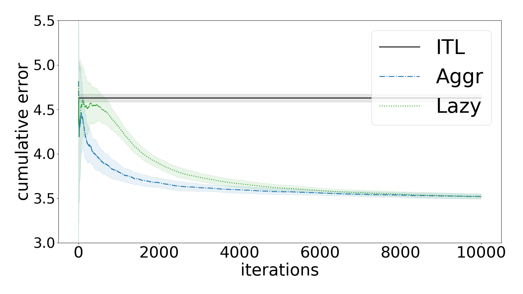
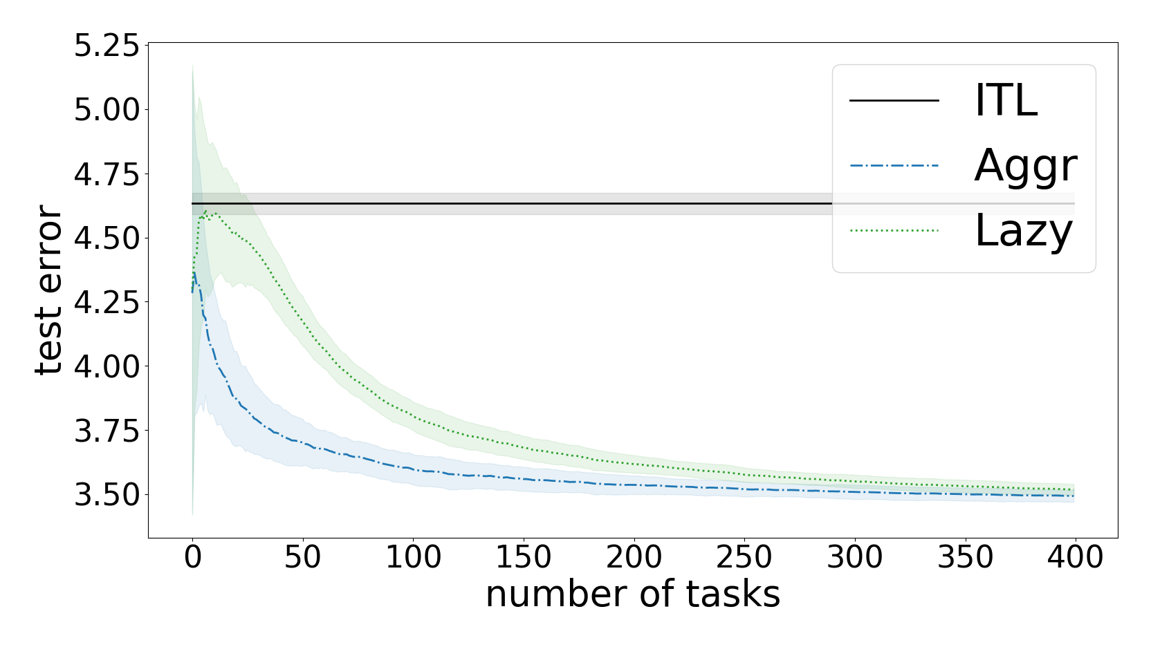
In this setting, we compared the performance of independent task learning (ITL) (running the unbiased variant of Alg. 3 over each task), our aggressive method in Alg. 4 (Aggr) and its lazy version in Alg. 5 in App. D (Lazy).
In the experiments below, we noticed that the variants of our methods estimating the magnitude by the refined coin betting algorithm in [10, Alg. ] returned a more readable plot w.r.t. the variants described in our theory using the KT algorithm in Alg. 1. For this reason, we report below the results obtained using this more refined variant.
In Fig. 1 (top) we report the average across-tasks cumulative error for all the methods w.r.t. to an increasing number of datapoints/iterations. In Fig. 1 (bottom) we report their (statistical) average multi-task test errors for an increasing number of tasks. We measured the performance by the absolute loss and we set the initial wealths in our methods equal to , for both the within-task and the across-tasks algorithms. The results we got are in agreement with the theory. Our approaches lead to a substantial benefits w.r.t. ITL and they converge to the oracle (the algorithm with the best bias in hindsight) as the number of the observed datapoints/tasks increases. Moreover, coherently with our bounds, we observe that, the aggressive variant of our method presents faster rates w.r.t. its lazy counterpart.
Because of lack of space, in App. E, we report additional experiments investigating the sensitivity of our parameter-free methods w.r.t. to the initialization of the wealths and showing the effectiveness of our methods on two real datasets (the Lenk [20, 26] and the Schools [3] datasets). In such a case, we will report for completeness both the refined and the basic variant of our methods.
9 CONCLUSION
We developed a parameter-free method that learns a common bias shared by a growing sequence of tasks. The advantage of our method in comparison to solving the tasks independently manifests itself when the variance of target tasks’ weight vectors is sufficiently small. Our method is originally introduced in the non-statistical setting and it can be applied into an aggressive or lazy version. The aggressive version enjoys faster rates and it can be converted into a statistical multi-task learning method, while, the lazy method recovers standard rates, but it can be converted into a statistical meta-learning method, able to generalize across the tasks.
In the future it would valuable to investigate whether other multi-task learning methods based on different metrics and addressing different types of tasks’ relatedness (e.g. those based on a shared low dimensional representation [12, 34] or graph regularization [7, 16]) can be made parameter-free as well. Moreover, it would be interesting to understand if our analysis allows more cycles over the data as in [15] and if this can be beneficial. Finally, we also wonder whether our parameter-free approach can be beneficial to recent meta-learning frameworks [8] dealing with partial feedback scenarios [2].
Acknowledgements
This work was supported in part by SAP SE and by EPSRC Grant N. EP/P009069/1.
References
- [1] P. Alquier, T. T. Mai, and M. Pontil. Regret bounds for lifelong learning. In Proc. 20th International Conference on Artificial Intelligence and Statistics, pages 261–269, 2017.
- [2] J. Altschuler and K. Talwar. Online learning over a finite action set with limited switching. In Conference on Learning Theory, pages 1569–1573, 2018.
- [3] A. Argyriou, T. Evgeniou, and M. Pontil. Convex multi-task feature learning. Machine Learning, 73(3):243–272, 2008.
- [4] M.-F. Balcan, M. Khodak, and A. Talwalkar. Provable guarantees for gradient-based meta-learning. In International Conference on Machine Learning, pages 424–433, 2019.
- [5] J. Baxter. A model of inductive bias learning. J. Artif. Intell. Res., 12(149–198):3, 2000.
- [6] R. Caruana. Multitask learning. Machine Learning, 28(1):41–75, 1997.
- [7] G. Cavallanti, N. Cesa-Bianchi, and C. Gentile. Linear algorithms for online multitask classification. Journal of Machine Learning Research, 11:2901–2934, 2010.
- [8] L. Cella, A. Lazaric, and M. Pontil. Meta-learning with stochastic linear bandits. arXiv preprint arXiv:2005.08531, 2020.
- [9] N. Cesa-Bianchi, A. Conconi, and C. Gentile. On the generalization ability of on-line learning algorithms. IEEE Transactions on Information Theory, 50(9):2050–2057, 2004.
- [10] A. Cutkosky and F. Orabona. Black-box reductions for parameter-free online learning in banach spaces. In Conference on Learning Theory, pages 1493–1529, 2018.
- [11] G. Denevi, C. Ciliberto, R. Grazzi, and M. Pontil. Learning-to-learn stochastic gradient descent with biased regularization. In International Conference on Machine Learning, pages 1566–1575, 2019.
- [12] G. Denevi, C. Ciliberto, D. Stamos, and M. Pontil. Incremental learning-to-learn with statistical guarantees. In 34th Conference on Uncertainty in Artificial Intelligence 2018, pages 457–466, 2018.
- [13] G. Denevi, C. Ciliberto, D. Stamos, and M. Pontil. Learning to learn around a common mean. In Advances in Neural Information Processing Systems, pages 10190–10200, 2018.
- [14] G. Denevi, D. Stamos, C. Ciliberto, and M. Pontil. Online-within-online meta-learning. In Advances in Neural Information Processing Systems, pages 13089–13099, 2019.
- [15] H. Eichner, T. Koren, B. Mcmahan, N. Srebro, and K. Talwar. Semi-cyclic stochastic gradient descent. In International Conference on Machine Learning, pages 1764–1773, 2019.
- [16] T. Evgeniou, C. A. Micchelli, and M. Pontil. Learning multiple tasks with kernel methods. Journal of machine learning research, 6:615–637, 2005.
- [17] C. Finn, A. Rajeswaran, S. Kakade, and S. Levine. Online meta-learning. In International Conference on Machine Learning, pages 1920–1930, 2019.
- [18] E. Hazan. Introduction to online convex optimization. Foundations and Trends in Optimization, 2(3-4):157–325, 2016.
- [19] M. Khodak, M.-F. F. Balcan, and A. S. Talwalkar. Adaptive gradient-based meta-learning methods. In Advances in Neural Information Processing Systems, pages 5915–5926, 2019.
- [20] P. J. Lenk, W. S. DeSarbo, P. E. Green, and M. R. Young. Hierarchical bayes conjoint analysis: Recovery of partworth heterogeneity from reduced experimental designs. Marketing Science, 15(2):173–191, 1996.
- [21] N. Littlestone. From on-line to batch learning. In Proc. 2nd Annual Workshop on Computational Learning Theory, pages 269–284, 1989.
- [22] A. Maurer. Algorithmic stability and meta-learning. Journal of Machine Learning Research, 6:967–994, 2005.
- [23] A. Maurer. The rademacher complexity of linear transformation classes. In International Conference on Computational Learning Theory, pages 65–78, 2006.
- [24] A. Maurer, M. Pontil, and B. Romera-Paredes. Sparse coding for multitask and transfer learning. In International Conference on Machine Learning, pages 343–351, 2013.
- [25] A. Maurer, M. Pontil, and B. Romera-Paredes. The benefit of multitask representation learning. Journal of Machine Learning Research, 17(1):2853–2884, 2016.
- [26] A. M. McDonald, M. Pontil, and D. Stamos. New perspectives on k-support and cluster norms. Journal of Machine Learning Research, 17(155):1–38, 2016.
- [27] F. Orabona. Simultaneous model selection and optimization through parameter-free stochastic learning. In Advances in Neural Information Processing Systems, pages 1116–1124, 2014.
- [28] F. Orabona and D. Pál. Coin betting and parameter-free online learning. In Advances in Neural Information Processing Systems, pages 577–585, 2016.
- [29] A. Pentina and C. Lampert. A PAC-Bayesian bound for lifelong learning. In International Conference on Machine Learning, pages 991–999, 2014.
- [30] A. Pentina and R. Urner. Lifelong learning with weighted majority votes. In Advances in Neural Information Processing Systems, pages 3612–3620, 2016.
- [31] S. Shalev-Shwartz and S. Ben-David. Understanding Machine Learning: From Theory to Algorithms. Cambridge University Press, 2014.
- [32] M. Streeter and H. B. McMahan. No-regret algorithms for unconstrained online convex optimization. In Advances on Neural Information Processing Systems, pages 2402–2410, 2012.
- [33] S. Thrun and L. Pratt. Learning to Learn. Springer, 1998.
- [34] N. Tripuraneni, C. Jin, and M. I. Jordan. Provable meta-learning of linear representations. arXiv preprint arXiv:2002.11684, 2020.
APPENDIX
The appendix is structured in the following way. We start from reporting the proof of Prop. 3 in App. A. After that, we give the proof of Thm. 5 and Prop. 7 in App. B and App. C, respectively. Then, in App. D, we present and analyze the lazy variant of our method giving rise to a parameter-free statistical meta-learning method. Finally, in App. E, we report additional experiments we omitted in the main body because of lack of space.
Appendix A PROOF OF Prop. 3
See 3
-
Proof.
We start by observing that the first inequality in the statement holds by convexity of (see Asm. 1) and the fact that, by construction, . In order to show the second inequality, we just proceed as in the proof of [10, Thm. ]. Specifically, by definition of in Alg. 3 and the rewriting of as in Eq. 6–Eq. 7, we can write
(27) In order to get the desired statement, we bound the two terms above as follows. We start from observing that the first term above coincides with the regret of the sequence of scalars generated by Alg. 1 aiming at inferring the magnitude from the sequence of scalars . We also notice that, since by construction and since the Lipschitz and bounded inputs assumption in Asm. 1 implies (see [31, Lemma ]), then we have
(28) As a consequence, recalling the initial wealth of the algorithm, by Prop. 1, we have,
(29) Regarding the second term, we observe that the quantity coincides with the regret of the sequence generated by Alg. 2 on aiming at inferring the direction from the sequence of vectors , where, as observed above, by the Lipschitz and bounded inputs assumption in Asm. 1, we have . As a consequence, by Prop. 2, we have,
(30) Substituting Eq. 29 and Eq. 30 into Eq. 27, we get the desired statement, recalling that . ∎
Appendix B PROOF OF Thm. 5
See 5
-
Proof.
The first inequality in the statement holds by convexity of (see Asm. 1) and the fact . In order to show the second inequality, we proceed similarly to the proof of Prop. 3, but, we now take into account also the variation of the bias across the iterations. Specifically, by definition of and in Alg. 4 and the rewriting of in Eq. 17–Eq. 18 and in Eq. 10–Eq. 11, we can write
(31) In order to get the desired statement, we bound all the four terms above as follows. Regarding the first term, for any task , we observe that the quantity coincides with the regret of the sequence of scalars , generated by Alg. 1 aiming at inferring the within-task magnitude from the sequence of scalars . We also notice that, since by construction and since the Lipschitz and bounded inputs assumption in Asm. 1 implies (see [31, Lemma ]), then we have
(32) As a consequence, recalling the initial within-task wealth of the algorithm, by Prop. 1, we have,
(33) Regarding the second term, for any task , we observe that the quantity coincides with the regret of the sequence , generated by Alg. 2 on aiming at inferring the within-task direction from the sequence of vectors , where, as observed above, by Lipschitz and bounded inputs assumption in Asm. 1, we have . As a consequence, by Prop. 2, we have,
(34) We now observe that the third term coincides with the regret of the sequence of scalars , generated by Alg. 1 aiming at inferring the meta-magnitude from the sequence of scalars . We also notice that, since by construction and since the Lipschitz and bounded inputs assumption in Asm. 1 implies (see [31, Lemma ]), then we have
(35) As a consequence, recalling the initial meta-wealth of the algorithm, by Prop. 1, we have,
(36) Finally, we observe that the fourth term coincides with the regret of the sequence , generated by Alg. 2 on aiming at inferring the meta-direction from the sequence of vectors , where, as observed above, by Lipschitz and bounded inputs assumption in Asm. 1, . As a consequence, by Prop. 2, we have,
(37) Substituting Eq. 33, Eq. 34, Eq. 36 and Eq. 37 into Eq. 31, we get the desired statement, once one recalls that and . ∎
Appendix C Proof of Prop. 7
See 7
-
Proof.
During the proof we write explicitly the expectation
(38) By definition of in Eq. 24, we have that
(39) where, the first inequality follows by convexity of the function , in the third equality we have exploited the fact that depends only on the datasets and the first points of the -th dataset, , finally, in the fourth equality, since , we have used the identity
(40) Next, because of the i.i.d. sampling of the data, we observe that we can write
(41) The desired statement now follows from combining Eq. 39 and Eq. 41. ∎
As we already observed in the main body, looking at the proof above, we notice that the online-to-batch statement in Prop. 7 applies also to the ‘lazy’ version of our method reported in Alg. 5 in App. D. This allows us to convert also this lazy variant into a statistical (sub-optimal) multi-task learning method with a slower rate.
Appendix D LAZY VERSION OF OUR METHOD
In this section, we present and analyze the lazy variant of our method introduced in the main body. Specifically, after introducing the lazy method in Alg. 5, we give an across-tasks regret bound for it in Sec. D.1. After that, in Sec. D.2, we show how the method can be converted into a parameter-free statistical meta-learning method and we give a transfer risk bound for it.
D.1 ACROSS-TASKS REGRET BOUND
Alg. 5 contains the lazy version of Alg. 4. As already stressed in the main body, we call Alg. 5 ‘lazy’ since, differently from Alg. 4, the bias is updated only at the end of the task. In the following theorem, we give an across-tasks regret bound for Alg. 5.
Theorem 8 (Across-Tasks Regret Bound for Alg. 5).
-
Proof.
The proof exactly proceeds as the proof of Thm. 5. The first inequality in the statement holds by convexity of (see Asm. 1) and the fact that, by construction, . We now proceed with the proof of the second inequality. Specifically, by definition of and in Alg. 5, the rewriting of in Eq. 17–Eq. 18 and in Eq. 10–Eq. 11, proceeding in the same way as done in the proof of Thm. 5, one can show that the linear regret can be bounded by four contributions as follows:
(44) In order to get the desired statement, we bound all the four terms above as follows. The first two terms can be bounded as described in the proof of Thm. 5 in Eq. 33 and Eq. 34. We now observe that the third term coincides with the regret of the sequence of scalars , generated by Alg. 1 aiming at inferring the meta-magnitude from the sequence of scalars . We also notice that, since by construction and since the Lipschitz and bounded inputs assumption in Asm. 1 implies (see [31, Lemma ]), then we have
(45) As a consequence, recalling the initial meta-wealth of the algorithm, by Prop. 1, we have,
(46) Finally, we observe that the fourth term coincides with the regret of the sequence , generated by Alg. 2 on aiming at inferring the meta-direction from the sequence of vectors , where, as observed above, by Lipschitz and bounded inputs assumption in Asm. 1, . As a consequence, by Prop. 2, we have,
(47) Substituting Eq. 33, Eq. 34, Eq. 46 and Eq. 47 into Eq. 44, we get the desired statement, once one recalls that and . ∎
We observe that the bound above is equivalent to the bound for the method presented in [14], which requires, however, oracle tuning of two hyper-parameters. We observe also that the term A in the bound above is exactly equivalent to the term A in Thm. 5 for the aggressive version of the algorithm. However, as expected, in this lazy version, the term B is slower: it goes as , instead of the rate in Thm. 5 for the aggressive variant.
D.2 STATISTICAL META-LEARNING SETTING
In this section we show how we can convert Alg. 5 into a parameter-free statistical meta-learning algorithm and we present guarantees for it. We consider the statistical meta-learning framework described in [5, 22, 25]. More precisely, we assume that, for any , the within-task dataset is an independently identically distributed (i.i.d.) sample from a distribution (task) , and in turn the tasks are an i.i.d. sample from a meta-distribution (or environment) . Differently from the multi-task learning setting described in the main body, in the meta-learning setting here, we want to select an estimator which is able to generalize also across the tasks.
In this section, we will make explicit the dependency w.r.t. the dataset and the bias in the iteration generated by Alg. 3. The estimator we consider here is , the average of the iterates resulting from applying Alg. 3 to a test dataset with bias , a vector uniformly sampled among the bias vectors returned by our meta-algorithm in Alg. 5 applied to the training datasets . In this case, we want to study the performance of such an estimator in expectation w.r.t. the tasks sampled from the environment .
Formally, for any , we require that the corresponding true risk admits minimizers over the entire space and we denote by the minimum norm one. With these ingredients, we introduce the meta-learning oracle and, introducing the transfer risk of the estimator :
| (48) |
we give a bound on it w.r.t. the oracle . This is described in the following theorem.
Theorem 9 (Transfer Risk Bound for Alg. 5).
Let the same assumptions in Thm. 8 hold in the i.i.d. meta-learning statistical setting. Let as in Eq. 48, namely, the transfer risk of the average of the iterates generated by Alg. 3 with bias uniformly sampled among the bias vectors returned by Alg. 5 applied to the training datasets . Then, for any , in expectation w.r.t. the sampling of the datasets and the uniform sampling of ,
| (49) |
where
| (50) |
| (51) |
| (52) |
We observe that the bound above is composed by the expectation of the terms comparing in Thm. 8. This automatically derives from the fact that, as we will see in the following, the proof of the statement exploits the across-tasks regret bound given in Thm. 8 for Alg. 5 and, as described in the following proposition, online-to-batch conversion arguments [9, 21].
Proposition 10 (Online-To-Batch Conversion for Alg. 5).
Under the same assumptions in Thm. 6, the following relation holds
| (53) |
-
Proof.
In the following, we will explicitly write the expectation in the statement above as
(54) Writing more explicitly the expectation w.r.t. the uniform sampling and exploiting the definition of , we can write the following
(55) where, in the third equality we have exploited the fact that depends only on and the i.i.d. sampling of the datasets, in the inequality we have applied Jensen’s inequality to the convex function and, finally, in the last equality we have exploited the fact that depends only on the points and, consequently, thanks to the fact ,
(56) We now observe also that, by the i.i.d. sampling of the training data, we can write the following
(57) The desired statement derives from combining Eq. 55 and Eq. 57. ∎
We observe that the online-to-batch conversion above, similarly to [1, Thm. ] and [4, Thm. ], holds for a meta-parameter randomly sampled from the pool. In practice, this means that, when the number of training tasks is not known a priori, the method requires keeping in memory the meta-parameters estimated during the training phase in order to perform this sampling in the test phase. To give guarantees for an estimator which can be computed more efficiently by our method, as done in [11, 14], is still an open question. As already pointed out in the main body, we also observe that we did not manage to develop an online-to-batch conversion similar to the one above in Prop. 10 for the aggressive variant of our method in Alg. 4. In other words, we did not know whether it is possible to convert the aggressive variant of our method into a statistical meta-learning method able to generalize also to new tasks. This would imply faster rates going as for the second term in the bounds also for the meta-learning setting.
We now have all the ingredients necessary for the proof of Thm. 9.
Appendix E ADDITIONAL EXPERIMENTS
In this section we report additional experiments investigating the sensitivity w.r.t. the initial wealths and the effectiveness over real data of our methods. Also in these cases, we considered regression settings and we evaluated the errors by the absolute loss. In the plots below we reported also the (aggressive and lazy) variants of our parameter-free methods analyzed in our theory and using the KT algorithm in Alg. 1 to estimate the magnitudes. We will denote these variants with the subscript ‘KT’ to distinguish them from their counterparts estimating the magnitudes by the more refined variant of the coin betting algorithm described in [10, Alg. ].
E.1 SENSITIVITY W.R.T. THE INITIAL WEALTHS
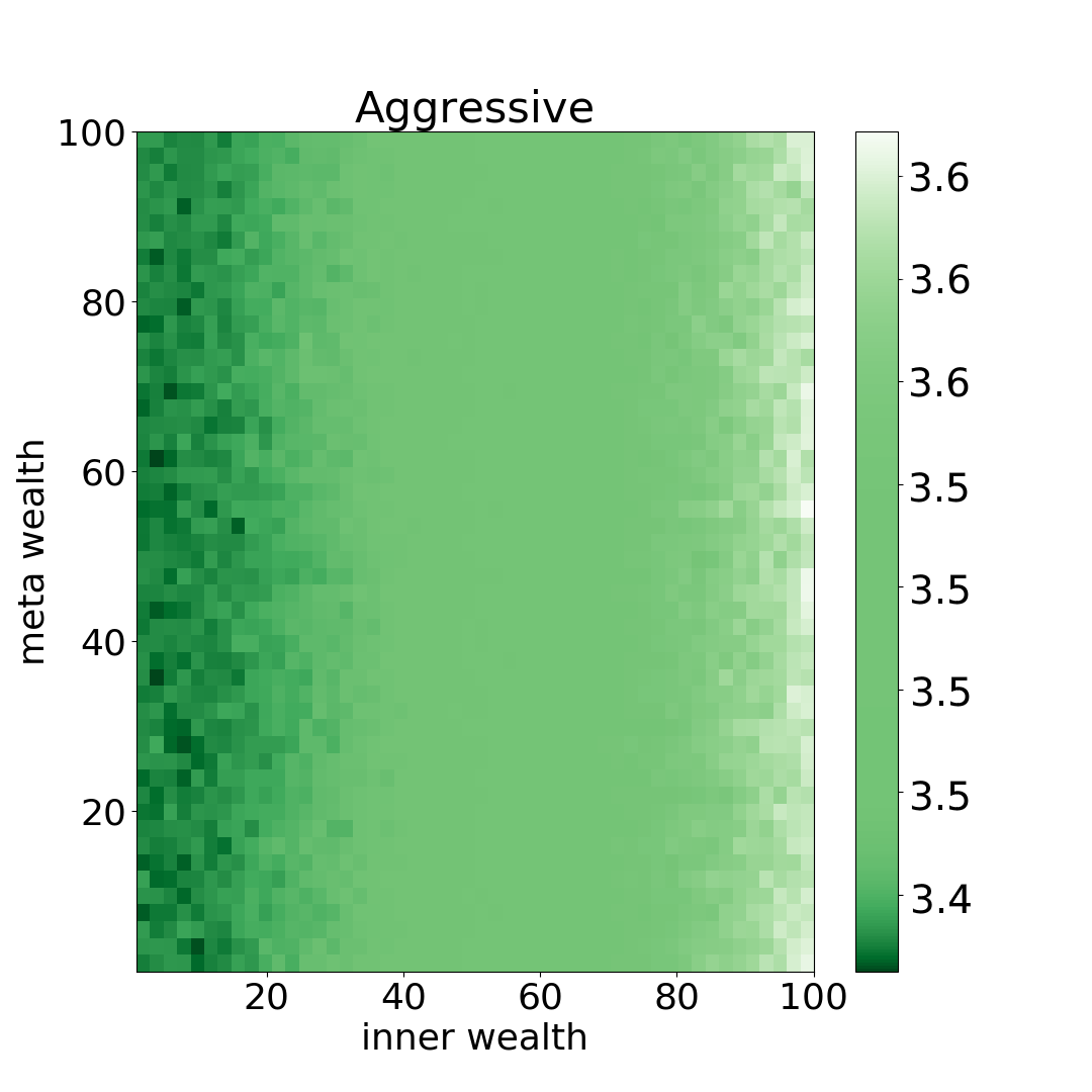
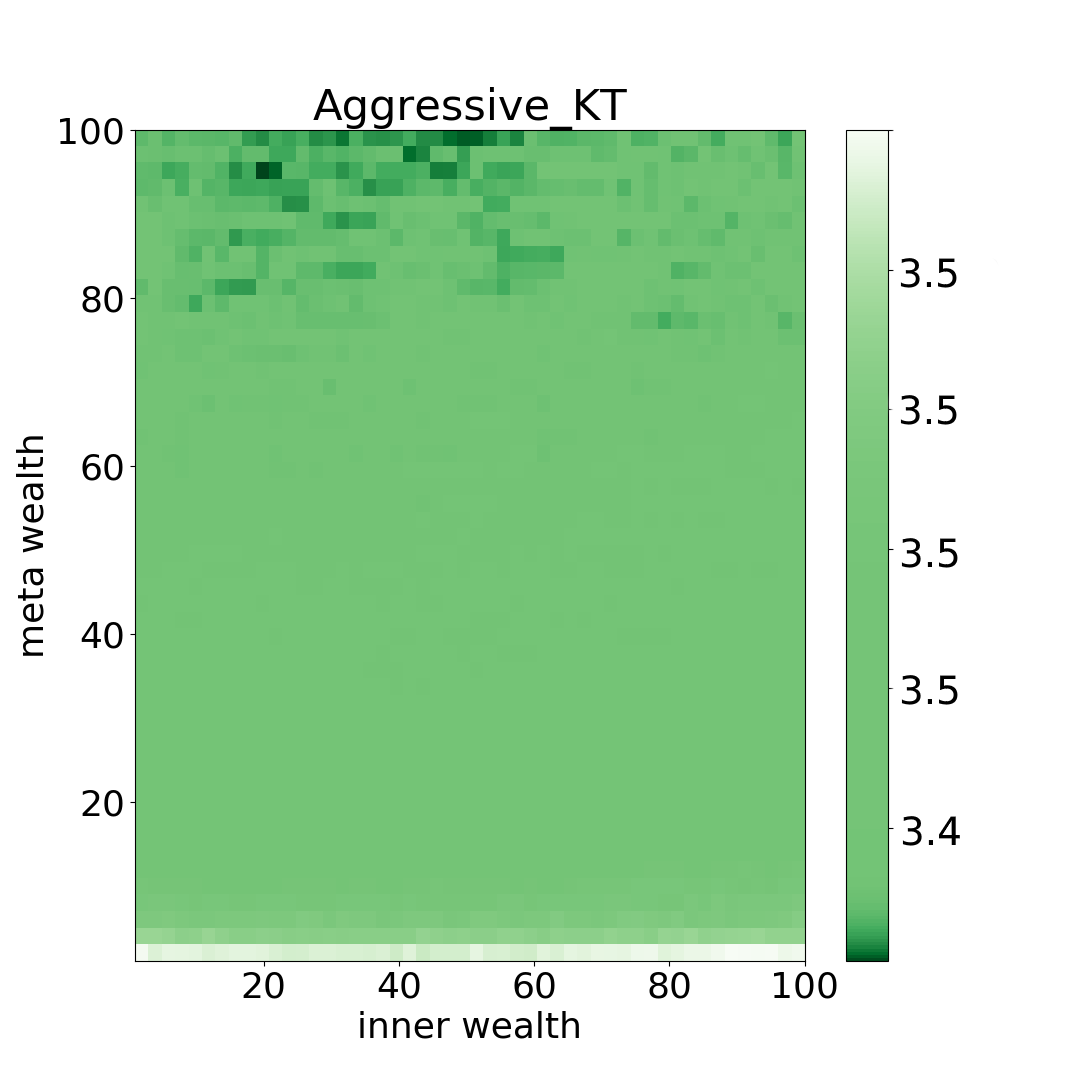
In order to investigate the sensitivity of our parameter-free methods w.r.t. to the initialization of the wealths, we ran the aggressive variants of our method on the same experimental setting of Fig. 1 (top) over a linearly spaced grid of (inner and outer/meta) initial wealths in the interval . In Fig. 2 we report the average across-tasks cumulative error we got at the end of the entire sequence of tasks for any value in the grid. From our results, we can observe that the performance of the method is quite stable and not much sensitive w.r.t. the initialization of the wealths. Hence, coherently to the single-task setting in [28], also in our multiple tasks methods, the choice of the initial wealths has a mild impact on the performance.
E.2 REAL EXPERIMENTS
We tested the performance of our methods also on two regression problems on the Lenk and the Schools datasets. Also in these cases, we set the initial wealths in our methods equal to , for both the inner and the outer algorithm. In the plots below, we used of the available datapoints for each task to train the inner algorithm. The remaining part was used to compute the test error of the inner algorithm in the statistical multi-task setting.
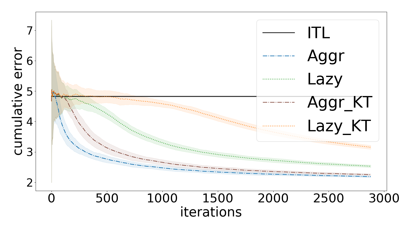
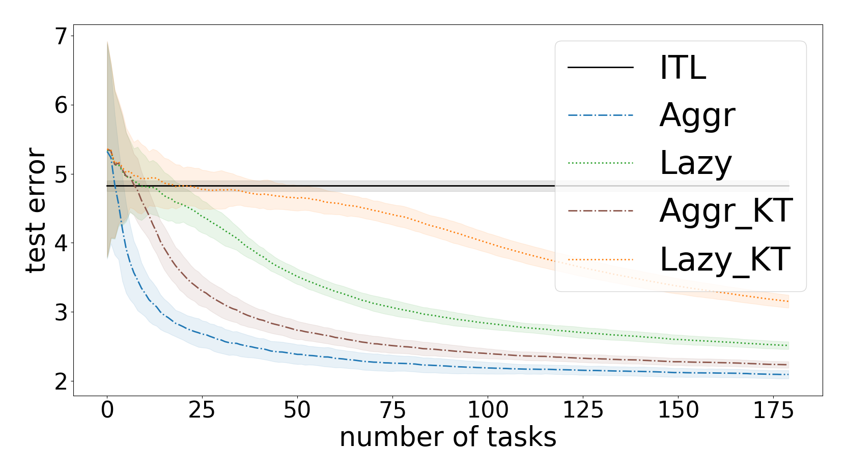
Lenk dataset. We considered the computer survey data from [20, 26], in which people (tasks) rated the likelihood of purchasing one of different personal computers. The input represents different computers’ characteristics, while the output is an integer rating between and . In Fig. 3 we report the average across-tasks cumulative error (left) and the average multi-task test error (right) for all the methods w.r.t. to an increasing number of datapoints/iterations or tasks. The results we got are in agreement with the synthetic experiments in the main body. Our parameter-free approaches significantly outperform ITL and they converge to the oracle (the algorithm with the best bias in hindsight) as the number of the observed datapoints/tasks increases. Again, the aggressive variants of our method present faster rates w.r.t. the corresponding lazy counterparts. We also observe that, in this setting, the KT variants of our parameter-free methods present a slightly slower convergence w.r.t. the corresponding refined variants.
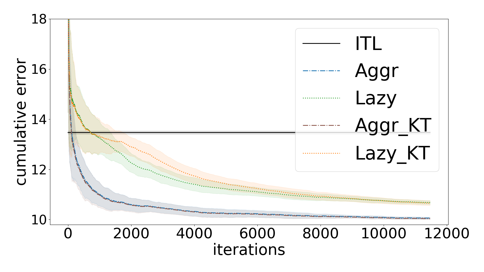
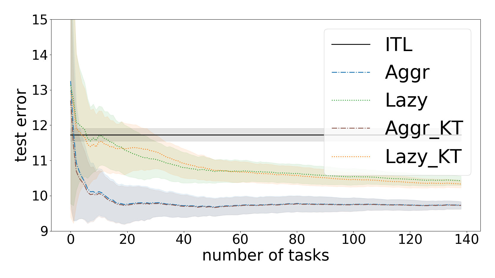
Schools dataset. We considered the Schools dataset [3], consisting of examination records from schools. Each school is associated to a task, individual students are represented by a features’ vectors , with , and their exam scores to the outputs. The sample size varies across the tasks from a minimum to a maximum . The results we got in Fig. 4 are coherent to the ones we described above for the Lenk dataset and they confirm the effectiveness of our method also on this dataset. In this case, we observe that, the convergence speed of the KT variants of our parameter-free methods is equivalent to the one of the corresponding refined variants.