The determination of the spin and parity of a vector-vector system

Abstract

We present a construction of the reaction amplitude for the inclusive production of a resonance decaying to a pair of identical vector particles such as $J/\psi J/\psi$, $\rho\rho$, $\phi\phi$, or $ZZ$. The method provides the possibility of determining the spin and parity of a resonance in a model-independent way. A test of the methodology is demonstrated using the Standard Model decay of the Higgs boson to four leptons.

I Introduction

The formation of hadronic matter is one of the few poorly understood parts of Quantum Chromodynamics (QCD). QCD is the fundamental theory of the strong interaction, but the quarks and gluons that constitute its degrees of freedom can only be resolved in hard processes with large momentum transfer. At lower energy scales where hadrons emerge, perturbative QCD is not applicable. The quark model (QM) Gell-Mann (1964); Godfrey and Isgur (1985) works well in classifying conventional hadronic states into mesons and baryons built from the constituent quarks bound in the confined potential. Hadrons beyond conventional mesons and baryons, such as glueballs containing constituent gluons, hybrid states containing quarks and gluons, and multiquark states, are referred to as exotic hadrons Klempt and Zaitsev (2007); Meyer and Swanson (2015). They are allowed by the QM, however they have not been seen experimentally until recently. Over the last decade overwhelming evidence has accumulated for exotic hadrons that include the observation of $XYZ$ states in the charmonium spectrum Godfrey and Olsen (2008), pentaquark states Aaij et al. (2015, 2019), as well as resonance-like phenomena from the triangle singularity in hadron scattering Alexeev et al. (2020). Nevertheless, the overall picture and the categorisation of these states remain unclear. The spin-parity of the observed exotic hadrons is a critical part of the formation puzzle. In most cases it can be accessed experimentally but the separation of the different spin-parity hypotheses is often rather cumbersome and requires a case-by-case treatment. In this paper we address the problem of the spin-parity assignment for a system of two identical vectors that decay to a pair of leptons or a pair of scalar particles.

Amongst the many applications of the presented framework, we note three in particular. First, it facilitates future studies of the resonance-like structure in the $J/\psi J/\psi$ spectrum recently reported by LHCb Aaij et al. (2020). The knowledge of its quantum numbers will help to understand the mechanism for the binding of four charm quarks Liu et al. (2019). Second, it can be applied in investigations of the central exclusive production (CEP) of vector-meson pairs. The colour-free gluon-rich production mechanism of CEP makes the $\rho\rho$ Armstrong et al. (1989); Abatzis et al. (1994); Österberg (2014) and $\phi\phi$ Barberis et al. (2000); Lebiedowicz et al. (2019) channels particularly suited to searches for glueballs. The proposed approach sets the ground for a complete partial wave analysis of the high statistics CEP of four scalar mesons that should be possible with modern LHC data. Third, one finds the same vector-vector signature in the Standard Model (SM) decay of the Higgs boson, $H\to ZZ$. In studies of the spin-parity quantum numbers of the Higgs boson performed by both the ATLAS Aad et al. (2013) and CMS Chatrchyan et al. (2013a) collaborations, to reach the conclusion that the observed Higgs boson is consistent with the $0^{+}$ hypothesis, several phenomenological models were compared using the combined datasets from several decay channels. In contrast, here we discuss the anatomy of an assumption-free approach.

The two key constraints that determine the decay properties are parity conservation and permutation symmetry. One consequence of these constraints is the Landau-Yang theorem Yang (1950); Landau (1948), which states that a massive boson with $J^{P}=1^{\pm}$ cannot decay into two on-shell photons. The statement follows naturally from the general equations we provide. Moreover, the extension of the selection rule to all natural quantum numbers with odd spin is easily obtained. A parity-signature test for a signal in the $\phi\phi$ system has been discussed in the past by several authors Chang and Nelson (1978); Trueman (1978). We derive results consistent with previous work using modern conventions on the state vectors and rotation matrices. In addition, we suggest exploring the spin-parity hypothesis using the full power of multidimensional test statistics.

The paper is organized as follows. The reaction amplitude is presented in Sec. II. In Sec. III the symmetry constraints are discussed. We propose a test statistic discriminator in Sec. IV, and demonstrate the method on the SM $H\to ZZ$ decay in Sec. V. Conclusions are presented in Sec. VI.

II Angular amplitude

We focus on the inclusive production process $pp^{\prime}\to X+\dots$, where $X$ is a resonance decaying to two vector mesons. Although the vector mesons are identical, it is convenient to distinguish them in the reaction amplitude calling them $V_{1}$ and $V_{2}$. In that way, we can make sure that the amplitude is symmetric under the permutation of indices $1$ and $2$. When the decay modes of the two vectors are identical, namely $X\to V(l_{1}^{+}l_{1}^{-})V(l_{2}^{+}l_{2}^{-})$, one needs to account for the symmetrized process $X\to V(l_{1}^{+}l_{2}^{-})V(l_{1}^{+}l_{2}^{-})$ and the interference between the two decay chains. For narrow resonances, the interference is minor and is neglected in the following discussion. The calculation of interference effects lies beyond the scope of this paper.

The production frame is set up in the rest frame of $X$ as a plane that contains the three-vectors of the production reaction, i.e.  $\vec{p}$ and $\vec{p}\,^{\prime}$. The normal to the plane gives the $y$ axis ($\vec{p}\,^{\prime}\times\vec{p}$) as shown in Fig. 1. The Gottfried-Jackson (GJ) frame is used to define the $x$ and $z$ axes in the production plane Gottfried and Jackson (1964), where the $z$ axis is defined along the direction of $\vec{p}$. The choice of $x$ and $z$ axes is not unique: two other common definitions of the production frame are the helicity (HX) frame, where the $z$ axis is defined by the direction of motion of $X$ itself in the lab frame Jacob and Wick (1959), and the Collins-Soper (CS) frame in which $z$ is defined by the bisector of the angle between $\vec{p}$ and $\vec{p}\,^{\prime}$ Collins and Soper (1977).

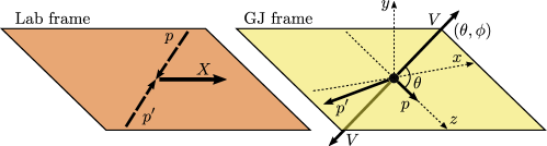
Figure 1: Schematic view of the production kinematics of the $X$ state in $pp$ collisions. The Gottfried-Jackson frame is used: the axes are defined in the rest frame of $X$ by the vectors of the beam particles: $\vec{z}=\vec{p}/|\vec{p}|$, $\vec{y}=\vec{p}^{\prime}\times\vec{p}/|\vec{p}^{\prime}\times\vec{p}|$, $\vec{x}=\vec{y}\times\vec{z}$. The spherical angles $(\theta,\phi)$ are the angles of one of the two decay vectors in the GJ frame. The black arrows shows the three-vectors of the particles. The three-momenta of the vector mesons are labeled by $V$.

We note that a negligibly small polarization is measured in the prompt production of charmonium (”head on” collisions) Aaij et al. (2013a); Chatrchyan et al. (2013b); Aaltonen et al. (2012); Aaij et al. (2013b); Sirunyan et al. (2018). In contrast, for peripheral processes, e.g. central exclusive production, a significant polarization is expected Pasechnik et al. (2011). Therefore we consider the general case of an arbitrary polarization of $X$.

The full kinematics of the decay is described by 6 angles: a pair of spherical angles $\Omega=(\theta,\phi)$ of the momentum of $V_{1}$ in the GJ frame, and two pairs of spherical angles $\Omega_{i}=(\theta_{i},\phi_{i})$, $i=1,2$ for the decays of the vector mesons $V_{i}$ in their own HX frames, as illustrated in Fig. 2. The angles $\phi_{i}$ can also be defined in the $X$ rest frame as shown in Fig. 2 since they are not affected by the boosts along the vector-meson directions of momentum. The spin of the decay particle $X$ defines the rotational properties of the system of decay products Mikhasenko et al. (2020). Every configuration of the three-momenta of the final-state particles in the $X$ rest frame can be considered as a solid body for which the orientation is described by three angles: the pair of spherical angles $(\theta,\phi)$ that describe the direction of $\vec{p}_{V_{1}}$, and $\phi_{1}$, the azimuthal direction of $l^{+}$ (see Fig. 1 and Fig. 2). We consider the decay $X\to V(l^{+}l^{-})V(l^{+}l^{-})$ in the following: small modifications needed for vector decays to scalars $X\to V(S^{+}S^{-})V(S^{+}S^{-})$ are given in Appendix A. The normalized differential cross section denoted by the intensity $I$ reads:

$$I(\Omega,\Omega_{1},\Omega_{2}) =(2J+1)\sum_{M,M^{\prime}}R_{M,M^{\prime}}\,\sum_{\nu,\nu^{\prime}}D_{M,\nu}^{J}(\phi,\theta,\phi_{1})D_{M^{\prime},\nu^{\prime}}^{J*}(\phi,\theta,\phi_{1})$$ (1)

$$\qquad\times\sum_{\xi_{1},\xi_{2}}^{\{-1,1\}}A^{\nu}_{\xi_{1},\xi_{2}}(\theta_{1},\theta_{2},\Delta\phi)A^{\nu^{\prime}*}_{\xi_{1},\xi_{2}}(\theta_{1},\theta_{2},\Delta\phi),$$

where the production and decay parts of the amplitude are explicitly separated. The spin of $X$ is denoted by $J$ and $M$ is its spin projection onto the $z$ axis. The definition of the Wigner D-function can be found in Ref. Collins and Soper (1977). The production dynamics are encapsulated in the polarization matrix $R_{M,M^{\prime}}$. The decay amplitude is denoted by $A^{\nu}_{\xi_{1},\xi_{2}}$, where $\nu$ is the difference of the vector-meson’s helicities, $-2\leq\nu\leq 2$, and $\xi_{i}$ is the difference of the two leptons’ helicities in the decay of $V_{i}$, $-1\leq\xi_{i}\leq 1$, $i=1,2$. As $\xi_{i}=0$ is suppressed by $m_{l}/m_{V}$ for the electromagnetic transition, we omit it in the summation. The remaining $V\to l^{+}l^{-}$ helicity couplings give an overall constant. The decay amplitude is described by the remaining three angles, $\theta_{1}$, $\theta_{2}$, and $\Delta\phi=\phi_{2}+\phi_{1}$ (see Fig. 2), and is given by

$$A^{\nu}_{\xi_{1},\xi_{2}}(\theta_{1},\theta_{2},\Delta\phi) =\frac{3}{2}\sum_{\lambda_{1},\lambda_{2}}\delta_{\nu,\lambda_{1}-\lambda_{2}}(-1)^{1-\lambda_{2}}H_{\lambda_{1}\lambda_{2}}d_{\lambda_{1},\xi_{1}}^{1}(\theta_{1})d_{\lambda_{2},\xi_{2}}^{1}(\theta_{2})e^{i\lambda_{2}\Delta\phi}.$$ (2)

The factor $(-1)^{1-\lambda_{2}}$ is related to the Jacob-Wick particle-2 phase convention Jacob and Wick (1959). Once the phase is factored out of the helicity coupling matrix $H_{\lambda_{1},\lambda_{2}}$, the symmetry relations for $H$ are significantly simpler as presented in the next section.

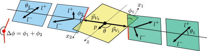
Figure 2: Schematic view of the $X\to V(l^{+}l^{-})\,V(l^{+}l^{-})$ decay kinematics. The central three planes show the orientation of the vector mesons in the $X$ rest frame. The rightmost plane shows the helicity angle $\theta_{1}$ for the $V_{1}$ decay in the rest frame of the two leptons while the leftmost plane shows the helicity for the $V_{2}$ decay in the rest frame of the other pair of leptons. The $x_{i}$ axes indicate the directions with respect to which the azimuthal angles of the positive leptons are measured in the decays of the vector mesons.

III Symmetry constraints

The matrix of the helicity couplings is strictly defined by

$$H_{\lambda_{1},\lambda_{2}}=\left\langle JM;\lambda_{1},\lambda_{2}\right|\hat{T}\left|JM\right\rangle,$$ (3)

where the bra-state is the projected two-particle state in the particle-2 phase convention, the ket-state is the decaying state with the defined $J$ and $M$ in the GJ frame, and $T$ is the interaction operator Martin and Spearman (1970); Collins (2009). The matrix is constrained by parity and permutation symmetry. Parity transformation relates the opposite values of the vectors’ helicities:

$$H_{\lambda_{1},\lambda_{2}}=P(-1)^{J}H_{-\lambda_{1},-\lambda_{2}},$$ (4)

with $P$ being the internal parity of $X$. The fact that the two vector mesons are identical relates the helicity matrix with the transposed one:

$$H_{\lambda_{1},\lambda_{2}}=(-1)^{J}H_{\lambda_{2},\lambda_{1}}.$$ (5)

The matrices of the helicity couplings are symmetric (anti-symmetric) for even (odd) spin $J$.

Table 1: Possible quantum numbers of the decaying particle $X$ separated into four groups with respect to the symmetry of the helicity matrix. The framed quantum numbers in the last column have additional restrictions due to the maximal value of the spin projection.

group	signum $s=(-1)^{J}$	naturality, $\epsilon=P(-1)^{J}$	explicit $J^{P}$
$I$	even($+$)	natural($+$)	$0^{+}$, $2^{+}$, $4^{+}$, $6^{+}$
${I\!I}$	even($+$)	unnatural($-$)	$0^{-}$, $2^{-}$, $4^{-}$, $6^{-}$
${I\!I\!I}$	odd($-$)	natural($+$)	$1^{-}$, $3^{-}$, $5^{-}$, $7^{-}$
${I\!V}$	odd($-$)	unnatural($-$)	$1^{+}$, $3^{+}$, $5^{+}$, $7^{+}$

The relations in Eq. (4) and Eq. (5) greatly reduce the number of free components of the helicity matrix, which can in general be written as

$$H =\begin{pmatrix}b&a&c\\ s\,a&d&\epsilon s\,a\\ \epsilon\,c&\epsilon\,a&\epsilon\,b\end{pmatrix}$$ (6)

where $a$, $b$, $c$, and $d$ are the helicity couplings, $\epsilon=P(-1)^{J}$ is the naturality of $X$, and the signum, $s$, determined by whether the spin of $X$ is odd or even, is given by $(-1)^{J}$. According to the values of $\epsilon$ and $s$, all possible quantum numbers $J^{P}$ are split into four groups as shown in Table 1. The helicity matrix for each groups is

$$I\Rightarrow \begin{pmatrix}b&a&c\\ a&d&a\\ c&a&b\end{pmatrix}, {I\!I}\Rightarrow \begin{pmatrix}b&a&\\ a&&-a\\ &-a&-b\end{pmatrix}, {I\!I\!I}\Rightarrow \begin{pmatrix}&a&\\ -a&&-a\\ &a&\end{pmatrix}, {I\!V}\Rightarrow \begin{pmatrix}&a&c\\ -a&&a\\ -c&-a&\end{pmatrix}.$$ (7)

In general, $a$, $b$, $c$, and $d$ are complex helicity couplings, however several of them vanish for specific groups: $c=d=0$ for group ${I\!I}$; $b=c=d=0$ for group ${I\!I\!I}$; and $b=d=0$ for group ${I\!V}$. There are three special cases for low $J^{P}$ where additional helicity couplings vanish due to the requirement $|\lambda_{1}-\lambda_{2}|\leq J$: $0^{+}$ in group $I$, for which $a=c=0$; $0^{-}$ in group ${I\!I}$ with $a=0$; and $1^{+}$ in group ${I\!V}$ with $c=0$.

The helicity matrices of different groups are orthogonal to each other given the scalar product

$$(H_{1}\cdot H_{2})=\mathrm{Tr}(H_{1}H_{2}^{\dagger}).$$ (8)

They produce generally different angular distributions except for a few degenerate cases discussed below. The scalar product in Eq. (8) is used to fix the normalization of $H$ and gives the relation between the helicity couplings:

$$(H\cdot H)=4|a|^{2}+2|b|^{2}+2|c|^{2}+|d|^{2}=1.$$ (9)

The form of the helicity matrices in Eq. (7) immediately leads to the conclusion of the Landau-Yang theorem Yang (1950); Landau (1948). For the decay of $X$ to a pair of real photons, $H_{0,\lambda}=H_{\lambda,0}=0$, as the photon cannot carry the longitudinal polarization, $\lambda=0$. Practically, this corresponds to setting to zero the second row and second column of the helicity matrix. The matrix of group ${I\!I\!I}$ completely vanishes, hence, mesons with odd-natural $J^{P}$ cannot decay to two real photons. The special case of group ${I\!V}$ with $c=0$ also vanishes so the decay of $J^{P}=1^{+}$ to two real photons is also forbidden.

It is often convenient to simplify the problem and consider only observables that are insensitive to the initial polarization. Once the decay plane orientation is integrated over in Eq. (1), the production polarization matrix $R$ collapses to its trace. Indeed, using the properties of the Wigner D-function and the normalization of $R$, $\mathrm{Tr}\,R=1$ we find that

$$I(\theta_{1},\theta_{2},\Delta\phi)=\int\frac{\mathrm{d}\Omega\,\mathrm{d}\phi_{1}}{8\pi^{2}}I(\Omega,\Omega_{1},\Omega_{2})=\sum_{\nu=-2}^{2}\sum_{\xi_{1},\xi_{2}}^{\{-1,1\}}|A^{\nu}_{\xi_{1},\xi_{2}}(\theta_{1},\theta_{2},\Delta\phi)|^{2}.$$ (10)

This intensity is a polynomial on trigonometric functions of the angles with the coefficients determined by the helicity couplings. For practical convenience we provide an explicit form of this expression calculated for the general matrix $H$:

$$I(\theta_{1},\theta_{2},\Delta\phi)=\sum_{i=1}^{6}c_{i}f_{i}(\theta_{1},\theta_{2},\Delta\phi)$$ (11)

where $f_{i}$ are normalized angular functions and $c_{i}$ are coefficients that depend on the helicity couplings. The functional forms for $f_{i}$ and $c_{i}$ are given in Table 2.

Table 2: Basis functions and coefficients for the three-dimensional angular distribution $I(\theta_{1},\theta_{2},\Delta\phi)$ as expressed in Eq. (11) for final states consisting of four leptons or four scalar particles.

$i$	angular functions, $f_{i}$	coeff. $c_{i}$ for $X\to V(l^{+}l^{-})V(l^{+}l^{-})$	coeff. $c_{i}$, for $X\to V(S^{+}S^{-})V(S^{+}S^{-})$
$1$	$9\sin^{2}{\left(\theta_{1}\right)}\sin^{2}{\left(\theta_{2}\right)}\sin^{2}{\left(\Delta\phi\right)}/2$	$-\epsilon|b|^{2}/2$	$-2\epsilon|b|^{2}$
$2$	$\sin{\left(\theta_{1}\right)}\sin{\left(\theta_{2}\right)}\cos{\left(\theta_{1}\right)}\cos{\left(\theta_{2}\right)}\cos{\left(\Delta\phi\right)}$	$(18\epsilon|a|^{2}s-9(\epsilon+1)\mathrm{Re}\,(b^{*}d))/4$	$18\epsilon|a|^{2}s-9(\epsilon+1)\mathrm{Re}\,(b^{*}d)$
$3$	$9\sin^{2}{\left(\theta_{1}\right)}\sin^{2}{\left(\theta_{2}\right)}/4$	$(2\epsilon|b|^{2}-8|a|^{2}+2|b|^{2}+2|c|^{2}+4|d|^{2})/4$	$2\epsilon|b|^{2}-8|a|^{2}+2|b|^{2}+2|c|^{2}+4|d|^{2}$
$4$	$3\sin^{2}{\left(\theta_{1}\right)}/2$	$(6|a|^{2}-3(|b|^{2}+|c|^{2}))/2$	$6|a|^{2}-6|d|^{2}$
$5$	$3\sin^{2}{\left(\theta_{2}\right)}/2$	$(6|a|^{2}-3(|b|^{2}+|c|^{2}))/2$	$6|a|^{2}-6|d|^{2}$
$6$	$1$	$9(|b|^{2}+|c|^{2})/2$	$9|d|^{2}$

There are potential cases where different hypotheses are not distinguishable. If $a$ is the only non-zero helicity coupling, the values of $\epsilon$ and $s$ that distinguish different groups enter only as the product $\epsilon s$. Hence, in this case, group-${I\!I}$ is indistinguishable from group-${I\!I\!I}$, and group-$I$ has the same angular distributions as group-${I\!V}$. Such vanishing of the helicity couplings, however, is an exceptional case and indicates some other symmetry or additional selection rule.

IV Testing hypotheses

Given a set of data corresponding to the decay of particle $X$, the questions arises as to how well its spin and parity can be determined using the angular distributions. The most powerful method for testing a spin-parity hypotheses is a multidimensional fit, which takes into account the correlations between the angular variables. We confine ourselves here to a three dimensional analysis removing the polarization degrees of freedom, although the discussion can be generalized to the full six-dimensional space treating the polarization as model parameters. To determine which group the particle belongs to, we define a test statistic

$$\mathrm{TS}_{G/G^{\prime}}=\mathcal{L}_{G}-\mathcal{L}_{G^{\prime}},$$ (12)

where $\mathcal{L}_{G}$ is the maximized value of the averaged log likelihood for group $G$ and is given by

$$\mathcal{L}_{G}=\frac{1}{N}\sum_{e=1}^{N}\log I((\theta_{1},\theta_{2},\Delta\phi)_{e}|G\{\hat{h}\})$$ (13)

where the sum runs over the $N$ events in the sample. The intensity is calculated for each event, assuming it belongs to group $G$ with the helicity couplings $\hat{h}$ that maximize the likelihood.

Alternatively, although formally less precise, one dimensional projections or moments can access the same quantities as can be seen from Eq. (11) and Table 2. Integrating the intensity over $\cos\theta_{1}$ and $\cos\theta_{2}$, the distribution of $\Delta\phi$ is given by

$$I(\Delta\phi)=1+\beta\cos(2\Delta\phi),$$ (14)

where $\beta=P|b|^{2}/(4|a|^{2}+2|b|^{2}+2|c|^{2}+|d|^{2})$. The sign of the $\cos(2\Delta\phi)$ component in given by the parity. It is positive for quantum numbers of group $I$, and negative for those in group ${I\!I}$. The decays from groups ${I\!I\!I}$ and ${I\!V}$ would not show any $2\Delta\phi$ dependence since $b=0$ for them. The one-dimensional projection in $\cos\theta_{i}$, $i=1,2$ also provides useful information on the helicity couplings:

$$I(\cos\theta_{i}) =1+\zeta\,\frac{3\cos^{2}\theta_{i}-1}{2},\quad i=1,2.$$ (15)

with $\zeta=(|b|^{2}+|c|^{2}-|a|^{2}-|d|^{2})/(4|a|^{2}+2|b|^{2}+2|c|^{2}+|d|^{2})$. The value of $\zeta$ always falls into the range $[-1,1/2]$. Furthermore, $\zeta\geq-1/4$ for groups ${I\!I}$ and ${I\!V}$ while it must be equal to $-1/4$ for group ${I\!I\!I}$. Fig. 3 summarises the values possible for $\beta$ and $\zeta$ separated by group.

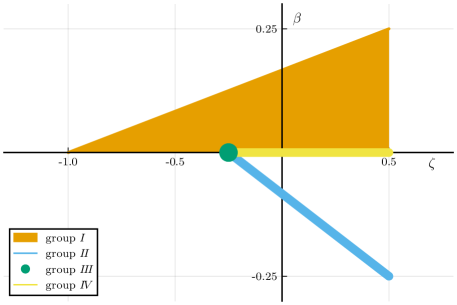
Figure 3: Allowed values of $\beta$ and $\zeta$ for the four spin-parity groups.

V Testing the Standard Model Higgs decay

The power of the test statistic defined in Eq. (12) is demonstrated using simulated data for the decay of the Higgs boson. The form of the helicity matrix is found by considering the interaction term of the Higgs with the gauge bosons. The covariant amplitude for $H\to ZZ$ reads:

$$i\mathcal{M}^{H\to ZZ}=2i\frac{m_{Z}^{2}}{v}(\varepsilon_{1}^{*}\cdot\varepsilon_{2}^{*}),$$ (16)

where $m_{Z}$ is the mass of the $Z$ boson and $v$ is the vacuum expectation value of the Higgs field. Using the explicit expressions for the polarization $\varepsilon_{i}(\lambda_{i})$ vectors (see Appendix B), the special form of the matrix for group $I$ is

$$H^{H\to ZZ}=\frac{\mathbb{I}}{\sqrt{3}}+O(p^{2}/m_{Z}^{2}),$$ (17)

where $p=\sqrt{m_{H}^{2}-4m_{Z}^{2}}$ is the break-up momentum of the $Z$ boson in the rest frame of the Higgs boson. The identity matrix corresponds to the $S$-wave in the decay, while the $D$-wave is proportional to $p^{2}$ and is suppressed at the $ZZ$ threshold: furthermore, since one $Z$ must be virtual, there is a negligible contribution from the $D$ wave. In the tests presented here, we consider the decay channel $H\to Z(e^{+}e^{-})Z(\mu^{+}\mu^{-})$; for $Z$-boson decays to identical final states, the interference between the two decay chains must be included.

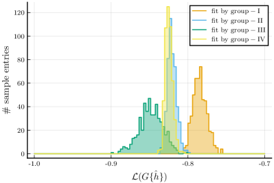
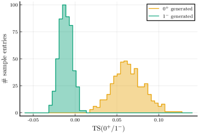
Figure 4: Left: Distribution of the maximized log-likelihood functions in a series of pseudoexperiments, each of which consists of 500 generated $H\to Z(e^{+}e^{-})Z(\mu^{+}\mu^{-})$ decays. Right: The test statistic $\mathrm{TS}(0^{+}|1^{-})$ for the sets generated with $J^{P}=0^{+}$ and $J^{P}=1^{-}$ are indicated by orange and green shading, respectively.

A sample of $500$ simulated $J^{P}=0^{+}$ events, corresponding to the helicity matrix in Eq. (17), were generated using a dedicated framework written in Julia jul . These events were fit for each group using the likelihood defined in Eq. (13). The results are shown in the left panel of Fig. 4 for a series of pseudoexperiments. One sees that the group-$I$ hypothesis has the highest likelihood on average. The separation is even larger once the test statistic from Eq. (12) is computed for each sample. The orange distribution in the right panel of Fig. 4 shows $\mathrm{TS}(0^{+}|1^{-})$, the comparison of the $J^{P}=0^{+}$ (group-$I$ hypothesis) with a selected alternative hypothesis that is taken to be $J^{P}=1^{-}$ (group-${I\!I\!I}$), and it is seen that the group-$I$ hypothesis is favoured. By contrast, a second set of pseudoexperiments was created simulating the decay of a “Higgs” boson with spin $1^{-}$. The same test statistic, $\mathrm{TS}(0^{+}|1^{-})$, is shown by the green distribution in the right panel of Fig. 4, and now generally disfavours the group-$I$ hypothesis.

Results from an analysis using the one-dimensional distributions given in Eq. (14) and (15) are shown in Fig. 5. The data correspond to a single pseudoexperiment with 500 simulated $H\to Z(e^{+}e^{-})Z(\mu^{+}\mu^{-})$ decays. Superimposed are the theoretical distributions expected from $J^{P}=0^{+},0^{-}$ and $1^{-}$; the data agree best with the $0+$ hypothesis with the values $\beta_{H}=1/6$ and $\zeta_{H}=0$. An ensemble of pseudoexperiments lead to estimations for $\beta$ and $\zeta$ that are shown as inset plots and compared to the theoretical values for three spin hypothesises. The width of the distributions indicate the precision of the determination. With a data sample of 500 events, the $0^{+}$ and $1^{-}$ hypotheses are separated by about twice the uncertainty on the experimental measurement, while in contrast, the multidimensional approach has a separation of about a factor four. This shows the improvement in experimental precision that can be achieved by combining and taking account of the correlations between the angular variables.

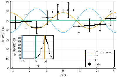
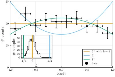
Figure 5: Distribution of the azimuthal angle $\Delta\phi$ (left) and of $\cos\theta_{1}$ (right) for the Higgs decay to $e^{+}e^{-}\mu^{+}\mu^{-}$ with a single sample of $500$ simulated events generated with the $J^{P}=0^{+}$ hypothesis. The orange lines are the expectation curves under the $J^{P}=0^{+}$ hypotheses with $b=d=1/\sqrt{3}$. The blue lines give the expected dependence for the quantum numbers $J^{P}=0^{+}$ (group ${I\!I}$). The distributions for $J^{P}=1^{-}$ are shown by the green lines. The inset plots show distribution of the parameters $\beta$ and $\zeta$ for an ensemble of pseudoexperiments. The coloured lines indicate the true values corresponding to each hypothesis.

VI Conclusion

An amplitude for the hadronic production and decay of two identical vector-mesons has been derived in a model-independent framework. For well-defined $J^{P}$ quantum numbers, the observed intensity has a non-trivial dependence on the angular variables that reflects the spin, parity and naturality of $J^{P}$. Four groups of $J^{P}$ can be distinguished based on angular distributions. We have given an explicit form of the expression for decays to leptons and scalar particles. Both projections of these distribution and a multidimensional discriminator have been investigated. We demonstrated the approach using the Standard Model Higgs decay to a pair of $Z$ bosons.

Appendix A Modifications for $X\to V(S^{+}S^{-})V(S^{+}S^{-})$

The amplitude requires a small modification when a system of four scalar particles is considered, e.g. $\rho(\pi^{+}\pi^{-})\rho(\pi^{+}\pi^{-})$ and $\phi(K^{+}K^{-})\phi(K^{+}K^{-})$. The decay matrix element in Eq. (2) reads:

$$A^{\nu}_{4S}(\theta_{1},\theta_{2},\Delta\phi) =3\sum_{\lambda_{1},\lambda_{2}}\delta_{\nu,\lambda_{1}-\lambda_{2}}(-1)^{1-\lambda_{2}}H_{\lambda_{1}\lambda_{2}}d_{\lambda_{1},0}^{1}(\theta_{1})d_{\lambda_{2},0}^{1}(\theta_{2})e^{i\lambda_{2}\Delta\phi}$$ (18)

where the decay $V\to S^{+}S^{-}$ proceeds in $P$-wave only. The variation in the $\Delta\phi$-dependence and $\cos\theta_{1}$ is more pronounced since there is no averaging over the spins of the final-state particles,

$$\beta_{(S)} =4\beta_{(l)}=\frac{2|b|^{2}}{4|a|^{2}+2|b|^{2}+2|c|^{2}+|d|^{2}}, \zeta_{(S)} =-2\zeta_{(l)}=\frac{-2|b|^{2}-2|c|^{2}+2|a|^{2}+2|d|^{2}}{4|a|^{2}+2|b|^{2}+2|c|^{2}+|d|^{2}},$$ (19)

with lower indices of $(S)$ and $(l)$ to indicate scalar and lepton particles, respectively.

Appendix B Polarization vectors

To translate the covariant expression in Eq. (16) to a helicity amplitude, the explicit expressions for the polarization vectors are used:

$$\varepsilon_{z}^{\mu}(\pm 1) =\frac{1}{\sqrt{2}}\left(0,\mp 1,-i,0\right), \varepsilon_{z}^{\mu}(0) =\frac{1}{m_{Z}}\left(p,0,0,E\right),$$ (20)

where $E$, $p$, and $m_{Z}$ are the energy, momentum, and mass of the $Z$ boson, respectively. The general expressions for the rotational vectors follow:

$$\varepsilon_{1}(\lambda) =R_{z}(\phi)R_{y}(\theta)\varepsilon_{z}(\lambda),$$ (21)

$$\varepsilon_{2}(\lambda) =(-1)^{1-\lambda}R_{z}(\phi)R_{y}(\theta)R_{y}(\pi)\varepsilon_{z}(\lambda),$$ (22)

where $R_{y}(\phi)R_{y}(\theta)$ is a product of the three-dimensional rotation matrices that transforms the vector $(0,0,1)$ to the direction $(\sin\theta\cos\phi,\,\sin\theta\sin\phi,\,\cos\theta)$. The second particle obtains an additional rotation by $\pi$ about the $y$ axis since we use the particle-2 phase convention.

References

- Gell-Mann (1964) M. Gell-Mann, Phys. Lett. 8, 214 (1964).
- Godfrey and Isgur (1985) S. Godfrey and N. Isgur, Phys. Rev. D 32, 189 (1985).
- Klempt and Zaitsev (2007) E. Klempt and A. Zaitsev, Phys. Rept. 454, 1 (2007), eprint 0708.4016.
- Meyer and Swanson (2015) C. Meyer and E. Swanson, Prog. Part. Nucl. Phys. 82, 21 (2015), eprint 1502.07276.
- Godfrey and Olsen (2008) S. Godfrey and S. L. Olsen, Ann. Rev. Nucl. Part. Sci. 58, 51 (2008), eprint 0801.3867.
- Aaij et al. (2015) R. Aaij et al. (LHCb), Phys. Rev. Lett. 115, 072001 (2015), eprint 1507.03414.
- Aaij et al. (2019) R. Aaij et al. (LHCb), Phys. Rev. Lett. 122, 222001 (2019), eprint 1904.03947.
- Alexeev et al. (2020) M. Alexeev et al. (2020), eprint 2006.05342.
- Aaij et al. (2020) R. Aaij et al. (LHCb) (2020), eprint 2006.16957.
- Liu et al. (2019) Y.-R. Liu, H.-X. Chen, W. Chen, X. Liu, and S.-L. Zhu, Prog. Part. Nucl. Phys. 107, 237 (2019), eprint 1903.11976.
- Armstrong et al. (1989) T. Armstrong et al. (WA76), Phys. Lett. B 228, 536 (1989).
- Abatzis et al. (1994) S. Abatzis et al. (WA91), Phys. Lett. B 324, 509 (1994).
- Österberg (2014) K. Österberg (TOTEM), Int. J. Mod. Phys. A 29, 1446019 (2014).
- Barberis et al. (2000) D. Barberis et al. (WA102), Phys. Lett. B 474, 423 (2000), eprint hep-ex/0001017.
- Lebiedowicz et al. (2019) P. Lebiedowicz, O. Nachtmann, and A. Szczurek, Phys. Rev. D 99, 094034 (2019), eprint 1901.11490.
- Aad et al. (2013) G. Aad et al. (ATLAS), Phys. Lett. B 726, 120 (2013), eprint 1307.1432.
- Chatrchyan et al. (2013a) S. Chatrchyan et al. (CMS), Phys. Rev. Lett. 110, 081803 (2013a), eprint 1212.6639.
- Yang (1950) C.-N. Yang, Phys. Rev. 77, 242 (1950).
- Landau (1948) L. Landau, Dokl. Akad. Nauk SSSR 60, 207 (1948).
- Chang and Nelson (1978) N.-P. Chang and C. Nelson, Phys. Rev. Lett. 40, 1617 (1978).
- Trueman (1978) T. Trueman, Phys. Rev. D 18, 3423 (1978).
- Gottfried and Jackson (1964) K. Gottfried and J. D. Jackson, Nuovo Cim. 33, 309 (1964).
- Jacob and Wick (1959) M. Jacob and G. Wick, Annals Phys. 7, 404 (1959).
- Collins and Soper (1977) J. C. Collins and D. E. Soper, Phys. Rev. D 16, 2219 (1977).
- Aaij et al. (2013a) R. Aaij et al. (LHCb), Eur. Phys. J. C 73, 2631 (2013a), eprint 1307.6379.
- Chatrchyan et al. (2013b) S. Chatrchyan et al. (CMS), Phys. Rev. Lett. 110, 081802 (2013b), eprint 1209.2922.
- Aaltonen et al. (2012) T. Aaltonen et al. (CDF), Phys. Rev. Lett. 108, 151802 (2012), eprint 1112.1591.
- Aaij et al. (2013b) R. Aaij et al. (LHCb), Phys. Lett. B 724, 27 (2013b), eprint 1302.5578.
- Sirunyan et al. (2018) A. M. Sirunyan et al. (CMS), Phys. Rev. D 97, 072010 (2018), eprint 1802.04867.
- Pasechnik et al. (2011) R. Pasechnik, A. Szczurek, and O. Teryaev, Phys. Rev. D 83, 074017 (2011), eprint 1008.4325.
- Mikhasenko et al. (2020) M. Mikhasenko et al. (JPAC), Phys. Rev. D 101, 034033 (2020), eprint 1910.04566.
- Martin and Spearman (1970) A. D. Martin and T. D. Spearman, Elementary-particle theory (North-Holland, Amsterdam, 1970), URL https://cds.cern.ch/record/102663.
- Collins (2009) P. D. B. Collins, An Introduction to Regge Theory and High-Energy Physics, Cambridge Monographs on Mathematical Physics (Cambridge Univ. Press, Cambridge, UK, 2009), ISBN 9780521110358, URL http://www-spires.fnal.gov/spires/find/books/www?cl=QC793.3.R4C695.
- (34) The JpsiJpsi framework implemented in Julia, Available at https://github.com/mmikhasenko/JpsiJpsi.jl.