Efficient ancilla-free reversible and quantum circuits
for the Hidden Weighted Bit function

Abstract

The Hidden Weighted Bit function plays an important role in the study of classical models of computation. A common belief is that this function is exponentially hard for the implementation by reversible ancilla-free circuits, even though introducing a small number of ancillae allows a very efficient implementation. In this paper we refute the exponential hardness conjecture by developing a polynomial-size reversible ancilla-free circuit computing the Hidden Weighted Bit function. Our circuit has size $O(n^{6.42})$, where $n$ is the number of input bits. We also show that the Hidden Weighted Bit function can be computed by a quantum ancilla-free circuit of size $O(n^{2})$. The technical tools employed come from a combination of Theoretical Computer Science (Barrington’s theorem) and Physics (simulation of fermionic Hamiltonians) techniques.

1 Introduction

The origins of the Hidden Weighted Bit function go back to the study of models of classical computation. This function, denoted $\mathsf{HWB}$, takes as input an $n$-bit string $x$ and outputs the $k$-th bit of $x$, where $k$ is the Hamming weight of $x$; if the input weight is $0$, the output is $0$. It is best known for combining the ease of algorithmic description and implementation by classical Boolean circuits with the hardness of representation by Ordered Binary Decision Diagrams (OBDDs) [1]—a popluar tool in VLSI [2]. The difference between logarithmic-depth implementations of $\mathsf{HWB}$ by circuits (recall that $\mathsf{HWB}\,{\in}\,NC^{1}$ but $\mathsf{HWB}\,{\not\in}\,AC^{0}$) and an exponential lower bound for the size of the OBDD [3] is startling two exponents. Relaxing the constraints on the type of Binary Decision Diagram considered or restricting the computations by circuits enables a multitude of implementations with polynomial cost [4].

The Hidden Weighted Bit function was first introduced in the context of reversible and quantum computations about 15 years ago by I. L. Markov and K. N. Patel (unpublished), and the earliest explicit mention dates to the year 2005 [5]. The original specification is irreversible, and required a slight modification to comply with the restrictions of reversible and quantum computations. Specifically, the Hidden Weighted Bit function was redefined to become the cyclic shift to the right by the input weight. We denote this reversible specification as $\mathbf{hwb}$. Formally, $\mathbf{hwb}(x)$ is defined as the cyclic shift of its input $x$ to the right by $W$ positions, where $W\,{=}\,x_{1}{+}x_{2}{+}\ldots{+}x_{n}$ is the Hamming weight of $x$. The following shows the truth table of $3$-input $\mathbf{hwb}$:

$x$	000	100	010	110	001	101	011	111
$\mathbf{hwb}(x)$	000	010	001	101	100	011	110	111

Since its introduction, $\mathbf{hwb}$ was used by numerous authors focusing on the synthesis and optimization of reversible and quantum circuits as a test case.

Despite a stream of improvements in the respective circuit sizes by various research groups [6, 7, 8, 9], the best known ancilla-free reversible circuits exhibit exponential scaling in the number of gates. The synthesis algorithms benefiting from the inclusion of additional gates, such as multiple-control multiple-target Toffoli, Fredkin, and Peres gates [5, 8, 10] also failed to find an efficient implementation without ancillae. In 2013, this culminated with the $\mathbf{hwb}$ receiving the designation of a “hard” benchmark function [11]. A recent asymptotically optimal synthesis algorithm over the library with NOT, CNOT, and Toffoli gates [12], introduced in the year 2015, was also unable to find an efficient ancilla-free implementation. An ancilla-free quantum circuit can be obtained by employing an asymptotically optimal quantum circuit synthesis algorithm such as [13], but the quantum gate count appears to remain exponential and larger than what is possible to obtain through the application of the asymptotically optimal reversible logic synthesis algorithm [12].

The introduction of even a small number of ancillae changes the picture dramatically. Just $O(\log(n))$ ancillary (qu)bits suffice to develop a reversible circuit with $O(n\log^{2}(n))$ gates [14]. Barrington’s theorem [15] allows one to obtain a polynomial-size reversible circuit using three ancillae. This polynomial-size three-ancilla reversible circuit can be obtained by computing the individual bits of the input weight through Barrington’s theorem, and using such bits logarithmically many times to control-SWAP the respective input (qu)bits into their desired positions. Finally, the existence of a polynomial-size quantum circuit using a single ancilla follows from [16].

State of the art, in both the classical reversible and quantum settings, thus points to an exponential difference in the gate count between circuits with no ancillae and circuits with a constant number of ancillae. In this paper, we demonstrate efficient implementations of the $\mathbf{hwb}$ function by ancilla-free reversible and quantum circuits, thereby reducing these exponential differences to polynomial. Specifically, our reversible ancilla-free circuit requires $O(n^{6.42})$ gates and our quantum ancilla-free circuit requires $O(n^{2})$ gates. These results refute the exponential hardness belief and remove $\mathbf{hwb}$ from the class of hard benchmarks.

We next sketch main ideas behind our ancilla-free circuits. We begin with the reversible circuit. Our construction works as follows. First, we show that the $n$-bit $\mathbf{hwb}$ function can be decomposed into a product of $O(n\log(n))$ gates denoted $C5(f(x);B)$, where $f(x)$ is a symmetric Boolean function and $B\,{\subset}\,x$ is a subset with $5$ input bits. The gate $C5(f;B)$ cyclically shifts the $5$-bit register $B$ if $f(x){=}1$, and does nothing when $f(x){=}0$. To implement $C5(f;B)$, we first break it down into a product of $6$ gates of the form $C5|_{M_{i}}(f(x{\setminus}B);B)$, where $i\,{\in}\,\{1,2,3,4,5,6\}$, each $M_{i}$ is a fixed set of Boolean $5$-tuples, and $f$ are symmetric Boolean functions. The gate $C5|_{M_{i}}$ restricts the operation of the corresponding gate $C5$ onto the set $M_{i}$ and simultaneously separates the set $B$ of bits being cycle-shifted from the set $x{\setminus}B$ controlling these shifts. This allows to employ Barrington’s theorem [15] to implement the gates $C5|_{M_{i}}(f(x{\setminus}B);B)$ in the ancilla-free fashion by expressing them as polynomial-size branching programs with the input $x{\setminus}B$ and computing into $B$. Each instruction in such program realizes a permutation of $5$-bit strings controlled by a single bit and it can thus be mapped into a reversible circuit over $6\,{=}\,5{+}1$ wires.

Next we introduce our quantum ancilla-free circuit. Let $U_{\mathbf{hwb}}$ be the $n$-qubit unitary operator implementing the $\mathbf{hwb}$ function. By definition, $U_{\mathbf{hwb}}|x\rangle=\mathsf{C}^{x_{1}+x_{2}+\ldots+x_{n}}|x\rangle$, where $\mathsf{C}$ is the cyclic shift of $n$ qubits. Suppose we can find an $n$-qubit Hamiltonian $H$ such that $\mathsf{C}\,{=}\,e^{iH}$ and $H$ commutes with the Hamming weight operator $W\,{=}\,\sum_{j=1}^{n}|1\rangle\langle 1|_{j}$. Then $U_{\mathbf{hwb}}=e^{iHW}$. Thus it suffices to construct a quantum circuit simulating the time evolution under the Hamiltonian $HW$. Since the cyclic shift $\mathsf{C}$ is analogous to the translation operator for a particle moving on a circle, the Hamiltonian $H$ generating the cyclic shift $\mathsf{C}$ is analogous to the particle’s momentum operator. This observation suggests that $H$ can be diagonalized by a suitable Fourier transform. We formalize this intuition using the language of fermions and the fermionic Fourier transform, which is routinely used in Physics and quantum simulation algorithms [17, 18]. The desired Hamiltonian $H$ such that $\mathsf{C}\,{=}\,e^{iH}$ is shown to have the form $H\,{=}\,V^{\dagger}H^{\prime}V$, where $V$ is a (modified) fermionic Fourier transform and $H^{\prime}$ is a simple diagonal Hamiltonian. We also show that $V$ commutes with the Hamming weight operator $W$, so that $U_{\mathbf{hwb}}\,{=}\,e^{iHW}\,{=}\,V^{\dagger}e^{iH^{\prime}W}V$. We demonstrate that each layer in this decomposition of $U_{\mathbf{hwb}}$ can be implemented by a quantum circuit of size $O(n^{2})$.

The rest of the paper is organized as follows. Section 2 introduces a simple modification of the known $O(n\log^{2}(n))$-gate $O(\log(n))$-ancilla reversible circuit that requires $O(n\log(n))$ gates and $O(\log(n))$ ancillary bits. Section 3 describes an $O(n^{6.42})$-gate ancilla-free reversible circuit. Section 4 reports an ancilla-free $O(n^{2})$-gate quantum circuit. These sections are independent of each other and can be read in any order. Appendices A and B prove technical lemmas stated in Section 4.

2 Reversible circuit of size $O(n\log n)$ using ancillas

We start with the description of a modification of the previously reported classical/reversible circuit that implements $\mathbf{hwb}$ with $O(n\log(n))$ gates and $O(\log(n))$ ancillae [14]. Compared to [14], our circuit features favorable asymptotics. However, it uses twice the computational/ancillary space.

Similarly to [14], we break down the computation into three stages:

1. Compute the input weight $W=x_{1}{+}x_{2}{+}\ldots{+}x_{n}$.

2. Apply controlled-SWAP gates to SWAP inputs into their correct position as specified by the $\mathbf{hwb}$.

3. Restore the value of ancillary register to ${\left|{0}\right\rangle}$ by appending the inverse of the stage 1.

Note that the stage 3. is omitted in [14], allowing a direct comparison to our circuit illustrated in Fig. 1. The difference between our construction and [14] is how we compute the input weight. Specifically, we use the same “plus-one” approach to calculate the weight into the ancillary register, however, we implement the integer increment function differently. Given input $x_{i}$, $1{\leq}i{\leq}n$, the resister $w_{1},w_{2},\ldots,w_{\lfloor\log(i)\rfloor{+}1}$, where the input weight is being computed into, and temporary storage $t_{1},t_{2},\ldots,t_{\lfloor\log(i)\rfloor{-}1}$, “increment by one” works as follows. If $i\,{=}\,1$, apply $\textsc{CNOT}(x1;w1)$. For $i\,{>}\,1$:

1. if $i{>}3$: apply Toffoli gate to ${\left|{x_{i},w_{1},t_{1}}\right\rangle}$; for $j$ from $2$ to $\lfloor\log(i)\rfloor{-}1$ apply the Toffoli gate $\textsc{Toffoli}(t_{j-1},w_{j};t_{j})$;

2. if $i\,{=}\,2$ or $i\,{=}\,3$ apply $\textsc{Toffoli}(x_{j},w_{1};w_{2})\textsc{CNOT}(x_{j};w_{1})$;
   else apply $\textsc{Toffoli}(t_{\lfloor\log(i)\rfloor-1},w_{\lfloor\log(i)\rfloor};w_{\lfloor\log(i)\rfloor+1})\textsc{CNOT}(t_{\lfloor\log(i)\rfloor-1};w_{\lfloor\log(i)\rfloor})$.

3. if $i{>}3$: for $j$ from $\lfloor\log(i)\rfloor{-}1$ down to $2$ apply the half adder, computed by the circuit $\textsc{Toffoli}(t_{j-1},w_{j};t_{j})\textsc{CNOT}(t_{j-1};w_{j})$. Apply $\textsc{Toffoli}(x_{i},w_{1};t_{1})\textsc{CNOT}(x_{i};w_{1})$.

In our implementation, the $t$ register is used to store necessary digit shifts. Advertised asymptotics follow by inspection of the above construction. We furthermore illustrated our circuit in Fig. 1 for $n{=}7$.

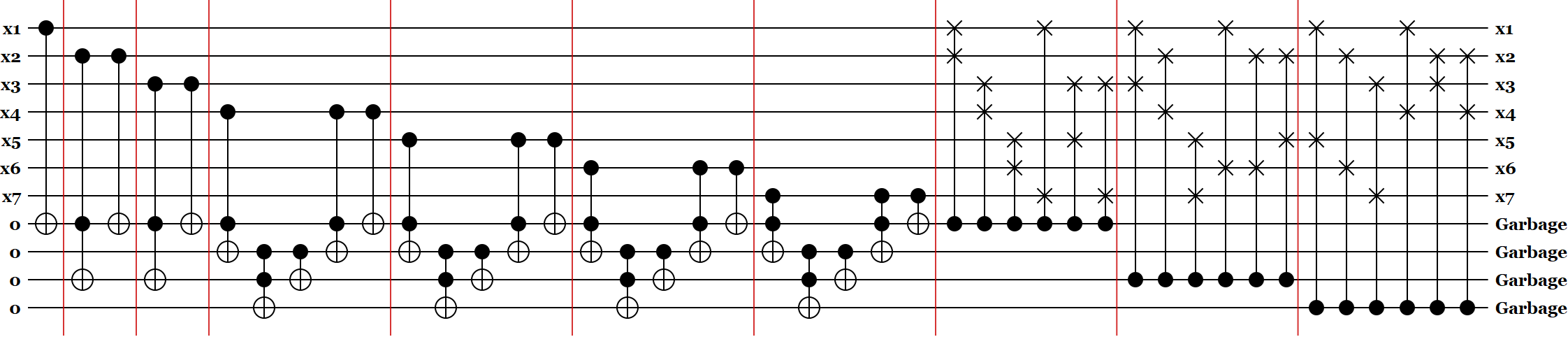
Figure 1: 10-stage reversible circuit applying the $7$-bit $\mathbf{hwb}$ to ${\left|{x_{1}x_{2}x_{3}x_{4}x_{5}x_{6}x_{7}w_{1}t_{1}w_{2}w_{3}}\right\rangle}$. Each of first $7$ $\textsc{CNOT}/\textsc{Toffoli}$ gate stages increments ${\left|{w_{1}w_{2}w_{3}}\right\rangle}$ by one depending on the value of input variable, next $3$ Fredkin gate stages perform controlled-SWAP. Vertical red lines separate these $10$ stages. Not shown is Garbage uncomputation that can be performed by appending the inversion of the weight calculation circuit ($\textsc{CNOT}/\textsc{Toffoli}$ gate part).

3 Ancilla-free reversible circuit of size $O(n^{6.42})$

In this section we show how to construct an ancilla-free classical reversible circuit of size $poly(n)$ implementing $\mathbf{hwb}$. We focus on $n\,{\geq}\,5$, noting that optimal circuits with $n$ up to $4$ are already known.

Let $n$ be the total number of bits, and $x=(x_{1},x_{2},...,x_{n})\in\{0,1\}^{n}$ be the input. In some discussions where it is convenient, we label these bits by the integers $\{0,1,\ldots,n{-}1\}\,{=}\,\mathbb{Z}_{n}$. Suppose $B\,{\subseteq}\,\mathbb{Z}_{n}$ is a subset of $5$ bits and $f:\{0,1\}^{n}\to\{0,1\}$ is a symmetric Boolean function (that is, $f(x)$ depends only on the Hamming weight of $x$). Define a reversible gate

$$C5(f;B):\,\{0,1\}^{n}\to\{0,1\}^{n},$$

where the output is obtained from the input $x$ by applying the cyclic shift to the register $B$ if $f(x){=}1$. Otherwise, when $f(x){=}0$, the gate does nothing. Note that, because the symmetric function $f$ does not depend on the order of the bits, $C5(f;B)$ is a permutation of the set $\{0,1\}^{n}$. Moreover, $C5(f;B)$ is an even permutation, since it is a product of length-$5$ cycles and each length-$5$ cycle is an even permutation.

Define $C(f;(i_{0},i_{1},...,i_{t-1}))$ to be a reversible gate that applies the cyclic shift of some $t$ bits defined by the cycle $(i_{0},i_{1},...,i_{t-1})$ (where $i_{0},i_{1},...,i_{t-1}\in\mathbb{Z}_{n}$ are all distinct) if the symmetric function $f$ evaluates to one and does nothing otherwise. We call $i_{0},i_{1},...,i_{t-1}$ the targets. We call a collection of $C$-type gates a layer when the sets of their targets do not overlap.

We next construct $\mathbf{hwb}$ by first expressing it as a circuit with the $C$-type gates, then breaking down the $C$-type gates into elementary reversible gates and $C5$-type gates, and finally expressing the $C5$-type gates in terms of the elementary reversible gates.

Lemma 1.

The $n$-bit $\mathbf{hwb}$ function can be implemented by an ancilla-free circuit with $\lfloor\log(n)\rfloor+1$ layers of $C$-type gates.

Proof.

We will create a circuit with $k$ layers numbered $0,1,...,\lfloor\log(n)\rfloor$. At each layer, the $C$ gates take the form $C(f_{k};*)$. Select the symmetric functions $f_{k}$ as follows: let $f_{k}(x)\,{=}\,1$ iff the $k$th power of $2$ in the binary expansion of the weight $W=x_{1}{+}x_{2}{+}...{+}x_{n}$ equals one. Note that $f_{k}$ are symmetric functions since the calculation of weight does not depend on the order the bits are added in. The function $\mathbf{hwb}$ can now be expressed as

$$\mathbf{hwb}=C^{2^{0}}((0,1,...,n{-}1);f_{0})C^{2^{1}}((0,1,...,n{-}1);f_{1})\cdots C^{2^{\lfloor\log(n)\rfloor}}((0,1,...,n{-}1);f_{\lfloor\log(n)\rfloor}).$$ (1)

For any $k=0,1,\dots,\lfloor\log(n)\rfloor$, let $g:=\text{GCD}(n,2^{k})$ and $C_{i}:=C(f_{k};(i,\,i{+}2^{k}\bmod n,\,...,\linebreak i{+}(\frac{n}{g}{-}1)2^{k}\bmod n))$. Then by elementary modular arithmetic,

$$C^{2^{k}}((0,1,...,n{-}1);f_{k})=C_{0}C_{1}\dots C_{g-1},$$

and the targets of any two distinct $C_{i}$ in this product do not overlap. This shows that each of the $\lfloor\log(n)\rfloor{+}1$ factors in Eq. (1) can be written as a layer of $C$-type gates. ∎

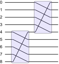
Figure 2: Implementation of the $9$-bit cyclic shift $C(f;(0,1,2,3,4,5,6,7,8))$ using the gates $C5(f;(4,5,6,7,8))$ and $C5(f;(0,1,2,3,4))$.

We next implement each of $\lfloor\log(n)\rfloor{+}1$ layers of cyclic shift gates in Lemma 1 as circuits with $O(n)$ $C5$-type gates by expressing the cycles $(i_{0},i_{1},...,i_{t-1})$ as products of length-$5$ cycles. Note that a length-$5$ cycle is always an even permutation and $(i_{0},i_{1},...,i_{t-1})$ is an odd permutation when $t$ is even. It is not possible to implement an odd permutation as a product of even permutations. However, with one exception, the $C$-type gates $C_{i}$ come in pairs (recall that their number, $g$, is a power of two) and thus they can usually be paired up to form an even permutation that can then be decomposed into a product of length-$5$ cycles. The one exception is the leftmost gate in Eq. (1), $C(f_{0};(0,1,...,n{-}1))$, when $n$ is even. We handle this case first.

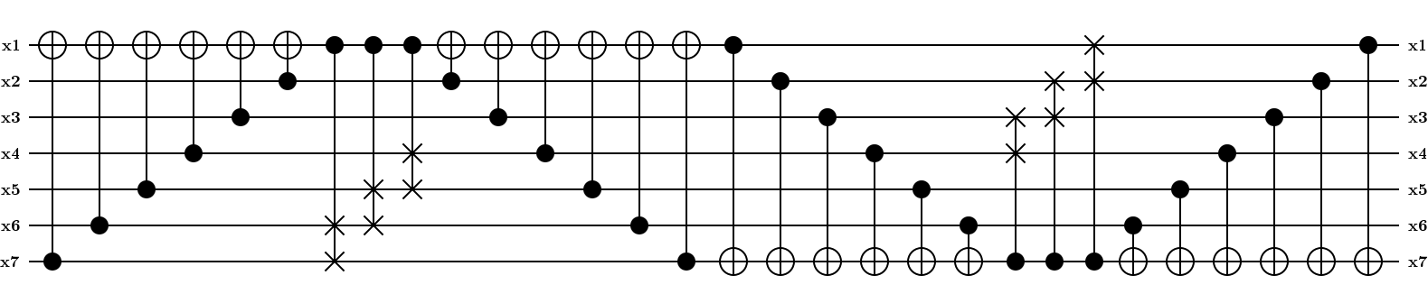
Figure 3: Implementation of $C(f_{0};(x_{1},x_{2},x_{3},x_{4},x_{5},x_{6},x_{7}))$, where $f_{0}(x)=x_{1}\oplus x_{2}\oplus x_{3}\oplus x_{4}\oplus x_{5}\oplus x_{6}\oplus x_{7}$.

Lemma 2.

$C(f_{0};(0,1,...,n{-}1))$ can be implemented by a reversible circuit with $O(n)$ elementary gates.

Proof.

The Boolean function $f_{0}(x)=x_{1}\oplus x_{2}\oplus...\oplus x_{n}$ can be implemented on the top bit to control all bit SWAPs on the bottom bits, and it can be implemented on the bottom bit to control all bit SWAPs on the top bits. The number of controlled-SWAP gates required is $n{-}1$, and the total number of the CNOT gates required to compute/uncompute the control register is $4(n{-}1)$. We illustrated this construction in Fig. 3 for $n{=}7$. ∎

Lemma 3.

For $n\,{\geq}\,5$:

1. for $t\,{\leq}\,4$, pairs of two $C(f;(i_{0},i_{1},...,i_{t-1}))$ gates can be implemented by an ancilla-free circuit using constantly many gates $C5(f;B)$;

2. for odd $t\,{>}\,4$ the $C(f;(i_{0},i_{1},...,i_{t-1}))$ gate can be implemented by an ancilla-free circuit using $O(t)$ gates $C5(f;B)$.

3. for even $t\,{>}\,4$ pairs of $C(f;(i_{0},i_{1},...,i_{t-1}))$ gates can be implemented by an ancilla-free circuit using $O(t)$ gates $C5(f;B)$;

Proof.

1. There are three cases to consider: $t\,{=}\,2$, $t\,{=}\,3$, and $t\,{=}\,4$.

• $C(f;(x_{1},x_{2}))$ and $C(f;(y_{1},y_{2}))$ can be implemented simultaneously by the circuit $C5(f;(y_{1},x_{1},y_{2},a,x_{2}))C5(f;(a,y_{1},x_{1},y_{2},x_{2}))$. This is equivalent to saying that the following permutation equality holds: $(x_{1},x_{2})(y_{1},y_{2})=(y_{1},x_{1},y_{2},a,x_{2})(a,y_{1},x_{1},y_{2},x_{2})$. Note that the bit ‘$a$’ can be found since $n\,{\geq}\,5$. We will show only the permutation equalities in the rest of the proof, since it is trivial to translate those to circuits.

• To implement a pair of gates $C(f;(x_{1},x_{2},x_{3}))$ and $C(f;(y_{1},y_{2},y_{3}))$ rely on the cycle product equality $(x_{1},x_{2},x_{3})(y_{1},y_{2},y_{3})=(x_{1},y_{1},x_{2},y_{2},y_{3})(x_{3},x_{1},y_{1},x_{2},y_{2})$.

• Cycles $(x_{1},x_{2},x_{3},x_{4})$ and $(y_{1},y_{2},y_{3},y_{4})$ can be obtained by the equality

  $$(x_{1},x_{2},x_{3},x_{4})(y_{1},y_{2},y_{3},y_{4})$$

  $$=(x_{1},x_{2})(x_{1},x_{3},x_{4})\cdot(y_{1},y_{2})(y_{1},y_{3},y_{4})$$

  $$=(x_{1},x_{2})(y_{1},y_{2})\cdot(x_{1},x_{3},x_{4})(y_{1},y_{3},y_{4}),$$

  where first and second part require two $C5$ gates each, as described in the cases $t\,{=}\,2$ and $t\,{=}\,3$, for a total of four $C5$ gates.

2. The goal is to develop a circuit with $C5$ gates implementing the gate $C(f;(0,1,...,t{-}1))$, where $t$ is odd. There are two cases to consider, $t\,{=}\,4p{+}1$ and $t\,{=}\,4p{+}3$.

Case 1: $t\,{=}\,4p{+}1,\;p\geq 1$. We want to implement the integer permutation given by the cyclic shift $(0,1,...,4p)$ by the cyclic shifts of length $5$. This can be done as follows,

$$(0,1,...,4p)=(4p-4,4p-3,4p-2,4p-1,4p)(4p-8,4p-7,4p-6,4p-5,4p-4)\cdots(0,1,2,3,4).$$

This decomposition uses $p$ length-5 cycles, resulting in the ability to implement $C(f;(0,1,...,t{-}1))$ gate using $p{=}\frac{t-1}{4}$ $C5(f;B)$ gates. This construction is illustrated in Fig. 2 for $n\,{=}\,9$.

Case 2: $t\,{=}\,4p{+}3,\;p\geq 1$. Use the formula

$$(0,1,...,4p{+}2)=(4p,4p{+}1,4p{+}2)\cdot(0,1,...,4p)$$

$$=(4p{+}2,4p,2,1,0)(4p{+}1,4p{+}2,0,1,2)\cdot(0,1,...,4p).$$

Since we already implemented $(0,1,...,4p)$ with $p$ $C5$ gates in Case 1 above, this implementation requires $\frac{t+5}{4}$ $C5$ gates.

3. The goal is to implement a pair of $C(f;(x_{1},x_{2},...,x_{t}))$ and $C(f;(y_{1},y_{2},...,y_{t}))$ where $t\,{>}\,4$ is even. Write

$$(x_{1},x_{2},...,x_{t})\cdot(y_{1},y_{2},...,y_{t})$$

$$=(x_{1},x_{2})(x_{1},x_{3},x_{4},...,x_{t})\cdot(y_{1},y_{2})(y_{1},y_{3},y_{4},...,y_{t})$$

$$=(x_{1},x_{2})(y_{1},y_{2})\cdot(x_{1},x_{3},x_{4},...,x_{t})\cdot(y_{1},y_{3},y_{4},...,y_{t})$$

Here, $(x_{1},x_{2})(y_{1},y_{2})$ requires two $C5$ gates per item 1. case $t\,{=}\,2$, and each of $(x_{1},x_{3},x_{4},...,x_{t})$ and $(y_{1},y_{3},y_{4},...,y_{t})$ requires $O(t)$ gates per item 2. ∎

Observe how the above proof implies that the number of $C5$ gates required to implement each of $C^{2^{k}}((0,1,...,n{-}1);f_{k})$ stages in Eq. (1) for $k=1,2,...,\lfloor\log(n)\rfloor$ is between $\frac{n}{4}+Const$ and $\frac{n}{2}+Const$. Thus, per Lemma 2, the total number of elementary and $C5$ gates required to implement $\mathbf{hwb}$ over $n$ qubits is between $\frac{n\log(n)}{4}+O(n)$ and $\frac{n\log(n)}{2}+O(n)$.

We next show how to implement $C5(f_{k};B)$ as a branching program, using Barrington’s theorem [15], by closely following the original proof. In preparation for using Barringon’s theorem, we first remove the dependence of the functions $f_{k}$ in $C5(f_{k};B)$ on the variables inside the set $B$, to allow the desired cyclic shift to be controlled by the values of $n{-}5$ variables outside the set $B$ itself. To accomplish this, note that $C5(f_{k};B)$ acts trivially on the strings $00000$ and $11111$; those can be ignored. This leaves $30$ non-fixed by the operation 5-bit strings that can be partitioned into six disjoint subsets $M_{1},M_{2},M_{3},M_{4},M_{5}$, and $M_{6}$, with $5$ strings each. Every subset $M_{i}$ contains $5$ cyclic shifts of some fixed $5$-bit string, and is defined as follows:

$$M_{1}:= \{10000,01000,00100,00010,00001\},$$ (2)

$$M_{2}:= \{01111,10111,11011,11101,11110\},$$

$$M_{3}:= \{11000,01100,00110,00011,10001\},$$

$$M_{4}:= \{10100,01010,00101,10010,01001\},$$

$$M_{5}:= \{00111,10011,11001,11100,01110\},$$

$$M_{6}:= \{01011,10101,11010,01101,10110\}.$$

We implement $C5(f_{k};B)$ by performing the cyclic shifts of a single subset $M_{i}$ per time.

First, let us introduce some more notations. Given a bit string $x\,{\in}\,\{0,1\}^{n}$, write $x=(y,b)$, where $b\,{\in}\,\{0,1\}^{5}$ is the restriction of $x$ onto the register $B$ and $y\,{\in}\,\{0,1\}^{n-5}$ is the rest of $x$. Let $w_{i}\,{\in}\,\{1,2,3,4\}$ be the Hamming weight of bit strings in $M_{i}$ (note that all strings in the same subset $M_{i}$ have the same weight). Define a Boolean function $f_{k,i}:\{0,1\}^{n-5}\to\{0,1\}$ such that $f_{k,i}(y){=}1$ iff $2^{k}$ appears in the binary expansion of $|y|{+}w_{i}$. Then

$$f_{k}(x)=f_{k}(y,b)=f_{k,i}(y)\quad\mbox{for any }b\in M_{i}.$$

Define a gate

$$C5|_{M_{i}}(f_{k};B):\,\{0,1\}^{n}\to\{0,1\}^{n}$$

that maps an input $x\,{=}\,(y,b)$ to an output $x^{\prime}\,{=}\,(y,b^{\prime})$ according to the following rules:

• if $f_{k,i}(y)\,{=}\,0$ then $b^{\prime}\,{=}\,b$;

• if $f_{k,i}(y)\,{=}\,1$ and $b\,{\notin}\,M_{i}$ then $b^{\prime}\,{=}\,b$;

• if $f_{k,i}(y)\,{=}\,1$ and $b\,{\in}\,M_{i}$ then $b^{\prime}\,{\in}\,M_{i}$ is obtained from $b$ by cyclically shifting the elements of $M_{i}$.

By definition, the cyclic shift of bits in the register $B$ can be realized by cyclically shifting elements of each subset $M_{i}$ for $i=1,2,3,4,5,6$. Thus

$$C5(f_{k}(x);B)=\prod_{i=1}^{6}C5|_{M_{i}}(f_{k}(y);B).$$ (3)

Here the order in the product does not matter because the gates $C5|_{M_{i}}(f_{k};B)$ pairwise commute. Note that the dependence of function $f_{k}$ on the variables inside the set $B$ has now been removed, and we can proceed to implementing $C5|_{M_{i}}(f_{k};B)$ as a branching program, and finally mapping the instructions used by the branching program into reversible gates.

Recall some relevant notation used in Barrington’s paper [15]. Let $S_{5}$ be the group of permutations of $5$ numbers, $\{1,2,3,4,5\}$. Given a $5$-tuple of distinct integers $a_{1},a_{2},a_{3},a_{4},$ and $a_{5}$, we write $(a_{1},a_{2},a_{3},a_{4},a_{5})$ to denote the $5$-cycle. Let $e$ be the identity permutation. A branching program of length $L$ with $m$ Boolean input variables $y_{1},y_{2},...,y_{m}$ is a list of instructions $\langle y_{i},\sigma_{i},\tau_{i}\rangle$ with $i=1,2,...,L$ and $\sigma_{i},\tau_{i}\in S_{5}$, such that $\sigma_{i}$ is applied if $y_{i}{=}1$, and $\tau_{i}$ is executed when $y_{i}{=}0$. Given a permutation $\sigma\in S_{5}$, the branching program is said to $\sigma$-compute a Boolean function $f(y)$ if executing the list of all instructions in the program results in $e$ (the identity permutation) for all inputs $y$ such that $f(y){=}0$ and permutation $\sigma$ for all inputs $y$ such that $f(y){=}1$.

Barrigton’s theorem asserts that any function in the class $\mathrm{NC}^{1}$ can be $(1,2,3,4,5)$-computed by a branching program of polynomial size [15]. We next specialize the proof of the theorem to explicitly develop a short branching program that $(1,2,3,4,5)$-computes the Boolean function $f_{k,i}(y)$. Recall that $f_{k,i}(y){=}1$ iff $2^{k}$ appears in the binary expansion of $y_{1}{+}y_{2}{+}\ldots{+}y_{n-5}{+}w_{i}$ with $w_{i}\in\{1,2,3,4\}$ being the weight of bit strings in $M_{i}$. It suffices to develop a branching program computing the Boolean function $f_{k}(y)$ with $y\in\{0,1\}^{m}$ and $m\,{=}\,n{-}5$ by appending at most two constant binary variables $1$ encoding $w_{i}$ to the bit string $y$.

While the original proof [15] explored the mapping of logarithmic-depth classical circuits over $\{\mathsf{AND},\mathsf{OR}\}$ library, we focus on the classical circuits over 3-input 1-output $\mathsf{MAJ}(a,b,c):=ab\oplus bc\oplus ac$ and $\mathsf{XOR}(a,b,c):=a\oplus b\oplus c$ gates. Recall that the library $\{\mathsf{MAJ},\mathsf{XOR}\}$ is universal for classical computations if constant inputs are allowed.

Lemma 4.

Suppose $y$ is an $m$-bit string and $f_{k}(y)$ is the $k$-th bit in the binary representation of $W=y_{1}{+}y_{2}{+}...{+}y_{m}$. The function $f_{k}(y)$ can be $(1,2,3,4,5)$-computed by a branching program of size $O(m^{5.42})$.

Proof.

First, we describe a logarithmic-depth classical circuit that computes functions $f_{k}(y)$ for the range of applicable values $k$, and second, report expressions for $\mathsf{MAJ}$ and $\mathsf{XOR}$ in the form of a branching program that can be used in the recursion [15, Proof of Theorem 1]. The length of the branching program computing $f_{k}(y)$ is upper bounded by taking the maximal length of the program implementing $\mathsf{MAJ}$ or $\mathsf{XOR}$ to the power of the circuit depth.

First, construct a classical circuit with $\mathsf{MAJ}$ and $\mathsf{XOR}$ gates that implements $f_{k}(y)$. To do so, we develop a circuit that computes all bits of the $W(y)$, and for the purpose of implementing a given single Boolean component, discard all gates that compute the bits we are not interested in. Such operation does not increase the depth of the circuit, and may, in fact, decrease it slightly.

To find $W(y)$, we employ a circuit consisting of two stages. First, compose a circuit of depth $\log_{3/2}(m)+O(1)$ with 3-input 2-output Full Adder gates $\mathsf{FA}(a,b,c):=(\mathsf{MAJ}(a,b,c),\mathsf{XOR}(a,b,c))$ by grouping as many triples of digits of same significance at each step as possible (note that $\mathsf{MAJ}$ and $\mathsf{XOR}$ are implemented in parallel). We finish this first stage when the output contains two $\log(m)$-digit integer numbers $u$ and $v$ such that $W=u\,{+}\,v$. To analyze this circuit, it is convenient to group all bits needing to be added into the smallest set of integer numbers, and count the reduction in the number of integers left to be added by treating layers of $\mathsf{FA}$ gates as Carry-Save Adders [19, 20]. A Carry-Save Adder is defined as the 3-integer into 2-integer adder, which is implemented by applying the Full Adders to the individual components of the three integer numbers at the input. Since the number of integers left to be added changes by a factor of $\frac{2}{3}$ at each step, and every step is implemented by a depth-$1$ $\mathsf{MAJ}/\mathsf{XOR}$ circuit, the depth of the first stage is $\log_{3/2}(m)\,{+}\,O(1)$. To find the individual components of $W(y)$, the second stage adds two $\log(m)$-digit integer numbers $u$ and $v$. This can be accomplished by any logarithmic-depth integer addition circuit in depth $O(\log\log(m))$, such as [21]. The total depth is thus $\log_{3/2}(m)\,{+}\,O(\log\log(m))$.

Next, construct $S_{5}$-programs computing the $\mathsf{MAJ}$ and $\mathsf{XOR}$ functions:

$$\langle z_{1},(1,4,3,2,5),e\rangle\;\;\langle z_{2},(1,3,5,4,2),e\rangle\;\;\langle z_{3},(1,2,5,3,4),e\rangle\;\;\langle z_{1},(1,2,3,4,5),e\rangle$$

$$\langle z_{2},(1,2,4,5,3),e\rangle\;\;\langle z_{3},(1,4,3,5,2),e\rangle\;\;\langle z_{1},(1,5,4,3,2),e\rangle\;\;\langle z_{1},(1,5,2,3,4),e\rangle$$

$$=\left\{\begin{array}[]{rcl}e&\mbox{if}&\mathsf{MAJ}(z_{1},z_{2},z_{3})=0\\ (1,2,3,4,5)&\mbox{if}&\mathsf{MAJ}(z_{1},z_{2},z_{3})=1,\\ \end{array}\right.$$ (6)

$$\langle z_{2},(1,2,3,5,4),e\rangle\;\;\langle z_{3},(1,2,4,5,3),e\rangle\;\;\langle z_{2},(1,3,5,4,2),e\rangle\;\;\langle z_{3},(1,4,5,3,2),e\rangle$$

$$\langle z_{1},(1,2,3,4,5),e\rangle\;\;\langle z_{2},(1,3,4,2,5),e\rangle\;\;\langle z_{2},(1,3,2,4,5),e\rangle\;\;\langle z_{3},(1,3,4,2,5),e\rangle$$

$$\langle z_{3},(1,3,2,4,5),e\rangle$$

$$=\left\{\begin{array}[]{rcl}e&\mbox{if}&\mathsf{XOR}(z_{1},z_{2},z_{3})=0\\ (1,2,3,4,5)&\mbox{if}&\mathsf{XOR}(z_{1},z_{2},z_{3})=1.\\ \end{array}\right.$$ (9)

The branching program that $(1,2,3,4,5)$-computes $f_{k}(y)$ is created by recursively replacing gates $\mathsf{MAJ}$ and $\mathsf{XOR}$ in the circuit constructed above with the branching programs Eq. (3) and Eq. (3), where each $z_{i}$ is either one of the primary input variables $y_{1},y_{2}\ldots,y_{m}$ or one of the intermediate variables in the circuit computing $f_{k}(y)$, until all instructions are controlled by constants and primary variables $y_{1},y_{2}\ldots,y_{m}$. The recoding of branches of the program $\tau$-computing a desired intermediate variable $z_{*}$ when $\tau{\neq}(1,2,3,4,5)$ (note how Eq. (3) and Eq. (3) $(1,2,3,4,5)$-compute the gates, but not $\tau$-compute them for arbitrary $\tau$) is accomplished in accordance with [15, Lemma 1]. The total length of the branching program is thus upper bounded by the size of longest branching program implementation of the basic gates used ($\mathsf{MAJ}$ and $\mathsf{XOR}$) raised to the power the depth of the circuit it encodes,

$$9^{\log_{3/2}(m)+O(\log\log(m))}=O(m^{5.4190225...}\log(m)^{O(1)})=O(m^{5.42}).$$

∎

We conclude this section by summarizing the main result in a Theorem.

Theorem 1.

The $n$-bit $\mathbf{hwb}$ function can be implemented by an ancilla-free reversible circuit of size $O(n^{6.42})$.

Proof.

First, implement each instruction $\langle z_{*},(a_{1},a_{2},a_{3},a_{4},a_{5}),e\rangle$ where $z_{*}$ is either a primary variable or a constant and the sets $\{a_{1},a_{2},a_{3},a_{4},a_{5}\}$ are defined per Eq. (2), using constantly many basic reversible gates. This can be accomplished by employing a reversible logic synthesis algorithm, e.g., [9]. Next, use Lemma 4 with $m=n{-}5$ and $x=y\,{\sqcup}\,B$ to implement all necessary $C5|_{M_{i}}(f_{k}(y);B)$ gates, using a branching program with

$$O\left(9^{\log_{3/2}(n-5)\,+\,O(\log\log(n-5))}\right)=O\left(9^{\log_{3/2}(n)\,+\,O(\log\log(n))}\right)$$

instructions. Each such branching program requires $O(9^{\log_{3/2}(n)+O(\log\log(n))})$ basic reversible gates since every instruction requires constantly many basic reversible gates. Use six $C5|_{M_{i}}(f_{k}(y);B)$ gates to implement one $C5(f_{k}(x);B)$ gate, using Eq. (3). Each $C5(f_{k}(x);B)$ thus costs $O(9^{\log_{3/2}(n)+O(\log\log(n))})$ basic reversible gates. Combine Lemma 1, Lemma 2, and Lemma 3 to implement $\mathbf{hwb}$ using $O(n\log(n))$ $C5(f_{k}(x);B)$ gates, implying the total basic reversible gate count of

$$O\left(9^{\log_{3/2}(n)\,+\,O(\log\log(n))}\cdot n\log(n)\right)=O\left(n^{6.4190225...}\log(n)^{O(1)}\right)=O(n^{6.42}).$$

∎

4 Ancilla-free quantum circuit of size $O(n^{2})$

Consider a register of $n$ qubits and let $\mathsf{C}$ be the cyclic shift operator,

$$\mathsf{C}|x_{1},x_{2},\ldots,x_{n-1},x_{n}\rangle=|x_{2},x_{3},\ldots,x_{n},x_{1}\rangle.$$

The hidden weighted bit function $U_{\mathbf{hwb}}$ may be written as

$$U_{\mathbf{hwb}}|x\rangle=\mathsf{C}^{x_{1}+x_{2}+\ldots+x_{n}}|x\rangle\quad\mbox{for all $x\in\{0,1\}^{n}$}.$$ (10)

In other words, $U_{\mathbf{hwb}}$ implements the $k$-th power of $\mathsf{C}$ on the subspace with the Hamming weight $k$. Here we show that $U_{\mathbf{hwb}}$ can be implemented by an ancilla-free quantum circuit of the size $O(n^{2})$. The circuit is expressed using Clifford gates and single-qubit $Z$-rotations.

Let

$$W=\sum_{j=0}^{n-1}|1\rangle\langle 1|_{j}$$ (11)

be the Hamming weight operator. Our starting point is

Lemma 5.

Suppose $\mathsf{C}=e^{iH}$ for some $n$-qubit Hamiltonian $H$ that commutes with $W$. Then

$$U_{\mathbf{hwb}}=e^{iHW}.$$ (12)

Proof.

Indeed, let ${\cal L}_{k}$ be the subspace spanned by all basis states $|x\rangle$ with the Hamming weight $k$. The full Hilbert space of $n$ qubits is the direct sum ${\cal L}_{0}\oplus{\cal L}_{1}\oplus\ldots\oplus{\cal L}_{n}$. Let us say that an operator $O$ is block-diagonal if $O$ maps each subspace ${\cal L}_{k}$ into itself. Since $H$ commutes with $W$, we infer that $H$ is block-diagonal. Therefore $HW$ and $e^{iHW}$ are also block-diagonal. Note that $HW$ and $kW$ have the same restriction onto ${\cal L}_{k}$. Thus $e^{iHW}$ and $e^{ikH}$ have the same restriction onto ${\cal L}_{k}$. By assumption, $e^{iH}=\mathsf{C}$. Thus $e^{iHW}$ and $\mathsf{C}^{k}$ have the same restriction onto ${\cal L}_{k}$. Likewise, $U_{\mathbf{hwb}}$ is block-diagonal and the restriction of $U_{\mathbf{hwb}}$ onto ${\cal L}_{k}$ is $\mathsf{C}^{k}$. We conclude that $U_{\mathbf{hwb}}$ and $e^{iHW}$ have the same restriction onto ${\cal L}_{k}$ for all $k$. Since both operators are block-diagonal, one has $U_{\mathbf{hwb}}=e^{iHW}$. ∎

We will construct a Hamiltonian $H$ satisfying conditions of Lemma 5 using the language of fermions and the fermionic Fourier transform [17, 18]. First, define fermionic creation and annihilation operators $a_{p}^{\dagger}$ and $a_{p}$ with $p\in\mathbb{Z}_{n}\equiv\{0,1,\ldots,n-1\}$ as

$$a_{p}^{\dagger}=\underbrace{Z\otimes Z\otimes\cdots\otimes Z}_{p}\otimes|1\rangle\langle 0|\otimes\underbrace{I\otimes I\otimes\cdots\otimes I}_{n-p-1}$$

$$a_{p}=\underbrace{Z\otimes Z\otimes\cdots\otimes Z}_{p}\otimes|0\rangle\langle 1|\otimes\underbrace{I\otimes I\otimes\cdots\otimes I}_{n-p-1}.$$

Here $Z=|0\rangle\langle 0|-|1\rangle\langle 1|$ is the Pauli-$Z$ operator.

Definition 1.

A Fermionic Fourier Transform is a unitary $n$-qubit operator $\mathsf{F}$ such that $\mathsf{F}|0^{n}\rangle=|0^{n}\rangle$ and

$$\mathsf{F}a_{p}\mathsf{F}^{\dagger}=\frac{1}{\sqrt{n}}\sum_{q\in\mathbb{Z}_{n}}e^{2\pi ipq/n}a_{q}\qquad\mbox{for all $p\in\mathbb{Z}_{n}$}.$$ (13)

Note that Eq. (13) uniquely specifies $\mathsf{F}$. Indeed, suppose $x\in\{0,1\}^{n}$ is a weight-$k$ basis state with ones at qubits $p_{1}<p_{2}<\ldots<p_{k}$. Then

$$\mathsf{F}|x\rangle=\mathsf{F}a_{p_{1}}^{\dagger}a_{p_{2}}^{\dagger}\cdots a_{p_{k}}^{\dagger}|0^{n}\rangle=\mathsf{F}a_{p_{1}}^{\dagger}\mathsf{F}a_{p_{2}}^{\dagger}\cdots a_{p_{k}}^{\dagger}\mathsf{F}^{\dagger}|0^{n}\rangle=\prod_{i=1}^{k}\mathsf{F}a_{p_{i}}^{\dagger}\mathsf{F}^{\dagger}|0^{n}\rangle.$$ (14)

Since each operator $\mathsf{F}a_{p_{i}}^{\dagger}\mathsf{F}^{\dagger}=(\mathsf{F}a_{p_{i}}\mathsf{F}^{\dagger})^{\dagger}$ is determined by Eq. (13), this uniquely specifies the action of $\mathsf{F}$ on the basis vectors $|x\rangle$. It will be important that $\mathsf{F}$ commutes with the Hamming weight operator $W$,

$$\mathsf{F}W=W\mathsf{F}.$$ (15)

Indeed, from Eqs. (13,14) one can see that $\mathsf{F}|x\rangle$ is a linear combination of states $a_{q_{1}}^{\dagger}a_{q_{2}}^{\dagger}\cdots a_{q_{k}}^{\dagger}|0^{n}\rangle$. Since $(a_{q}^{\dagger})^{2}=0$, the state $a_{q_{1}}^{\dagger}a_{q_{2}}^{\dagger}\cdots a_{q_{k}}^{\dagger}|0^{n}\rangle$ is non-zero only if all indices $q_{1},q_{2},\ldots,q_{k}$ are distinct. Such state has weight $k$. Thus $\mathsf{F}$ maps weight-$k$ states to linear combinations of weight-$k$ states proving Eq. (15).

We will use the following fact established by Kivlichan et al. [18].

Lemma 6.

The fermionic Fourier transform $\mathsf{F}$ on $n$ qubits can be implemented by a quantum circuit of size $O(n^{2})$. The circuit requires no ancillary qubits.

For completeness, we provide a simplified proof of Lemma 6 and an explicit construction of the quantum circuit realizing $\mathsf{F}$ in Appendix A. Now we are ready to define a Hamiltonian $H$ satisfying conditions of Lemma 5. Let

$$E=\frac{1}{2}(I+Z^{\otimes n})$$

be the projector onto the even-weight subspace. Define $n$-qubit Hamiltonians

$$H_{0}=\frac{2\pi}{n}\sum_{p\in\mathbb{Z}_{n}}p|1\rangle\langle 1|_{p},\qquad H^{\prime}=H_{0}+\frac{\pi}{n}WE,$$ (16)

and

$$H=V^{\dagger}H^{\prime}V\quad\mbox{where}\quad V=\mathsf{F}^{\dagger}e^{iH_{0}E/2}.$$ (17)

Lemma 7.

The Hamiltonian $H$ defined in Eq. (17) satisfies $C=e^{iH}$.

A proof of this lemma is given in Appendix B. A high-level intuition behind the definition of $H$ comes from the fact that $\mathsf{F}H_{0}\mathsf{F}^{\dagger}$ is the fermionic momentum operator. Note that $H=\mathsf{F}H_{0}\mathsf{F}^{\dagger}$ in the odd-weight subspace where $E\,{=}\,0$. The extra terms in the definition of $H$ are needed to change integer momentums (periodic boundary conditions) in the odd-weight subspace to half-integer momentums (anti-periodic boundary conditions) in the even-weight subspace. This accounts for the difference between the qubit cyclic shift and its fermionic analogue, as detailed in Appendix B.

From Eq. (15) one can see that $HW\,{=}\,WH$. Thus $H$ satisfies conditions of Lemma 5. Combining Lemma 5, Lemma 7, and noting that $VW\,{=}\,WV$ one arrives at

$$U_{\mathbf{hwb}}=e^{iHW}=e^{iV^{\dagger}H^{\prime}VW}=V^{\dagger}e^{iH^{\prime}W}V=e^{-iH_{0}E/2}\mathsf{F}e^{iH^{\prime}W}\mathsf{F}^{\dagger}e^{iH_{0}E/2}.$$ (18)

Here we used the well-known fact that $e^{iV^{\dagger}OV}=V^{\dagger}e^{iO}V$ for any Hermitian operator $O$ and any unitary $V$ (which can be verified by expanding the exponent using the Taylor series and noting that $(V^{\dagger}OV)^{p}=V^{\dagger}O^{p}V$ for all $p\geq 1$). We claim that each term in Eq. (18) can be implemented using $O(n^{2})$ two-qubit gates without ancillary qubits. By Lemma 6, the layers $\mathsf{F}$ and $\mathsf{F}^{\dagger}$ have gate cost $O(n^{2})$.

For the term $e^{iH_{0}E/2}$ and its inverse, we have the following lemma.

Lemma 8.

The operator $e^{iH_{0}E/2}$ can be implemented by a quantum circuit of size $O(n)$ without using ancillary qubits.

Proof.

If we set $\theta_{p}=p\pi/n$, then

$$e^{iH_{0}E/2}=R_{1}R_{2}\cdots R_{n-1},\quad\mbox{where }R_{p}=e^{i\theta_{p}|1\rangle\langle 1|_{p}E}.$$ (19)

The operator $|1\rangle\langle 1|_{p}E$ projects the subset of qubits $\mathbb{Z}_{n}{\setminus}\{p\}$ onto the odd-weight subspace. Note $p{\neq}0$ and let $C_{p}$ be a CNOT circuit that computes the parity of $\mathbb{Z}_{n}{\setminus}\{p\}$ into the qubit $0$,

$$C_{p}=\prod_{j\in\mathbb{Z}_{n}\setminus\{0,p\}}\textsc{CNOT}_{j,0}.$$

Then $|1\rangle\langle 1|_{p}E=C_{p}^{\dagger}|11\rangle\langle 11|_{0p}C_{p}$ and thus

$$R_{p}=C_{p}^{\dagger}e^{i\theta_{p}|11\rangle\langle 11|_{0p}}C_{p}.$$

Therefore, an individual $R_{p}$ is implemented with $O(n)$ gates, which suggests $e^{iH_{0}E/2}$ can be implemented with $O(n^{2})$ gates. However, we can improve this count by noting that for $p{\neq}q$

$$C_{p}C^{\dagger}_{q}=\textsc{CNOT}_{p,0}\textsc{CNOT}_{q,0}.$$ (20)

Thus, in fact, the product in Eq. (19) can be implemented with just $O(n)$ gates. ∎

We still need to implement the term $e^{iH^{\prime}W}=e^{iH_{0}W}e^{i(\pi/n)W^{2}E}$. The operator $e^{iH_{0}W}$ is a product of $O(n^{2})$ rotations $e^{i\theta|11\rangle\langle 11|}$ and $e^{i\theta|1\rangle\langle 1|}$. Although a naive implementation of $e^{i(\pi/n)W^{2}E}$ requires $O(n^{3})$ gates, we next show that a better implementation exists.

Lemma 9.

The operator $e^{i(\pi/n)W^{2}E}$ can be implemented by a quantum circuit of size $O(n^{2})$ without using ancillary qubits.

Proof.

First, note that

$$W^{2}E=2\sum_{\begin{subarray}{c}p,p^{\prime}\in\mathbb{Z}_{n}\\ 0<p<p^{\prime}\end{subarray}}|11\rangle\langle 11|_{pp^{\prime}}E+2\sum_{\begin{subarray}{c}p\in\mathbb{Z}_{n}\\ 0<p\end{subarray}}|11\rangle\langle 11|_{0p}E+\sum_{p\in\mathbb{Z}_{n}}|1\rangle\langle 1|_{p}E.$$ (21)

The terms in Eq. (21) commute. Therefore, we have, with arbitrary order within the products,

$$e^{i(\pi/n)W^{2}E}=\prod_{\begin{subarray}{c}p,p^{\prime}\in\mathbb{Z}_{n}\\ 0<p<p^{\prime}\end{subarray}}U_{pp^{\prime}}\prod_{\begin{subarray}{c}p\in\mathbb{Z}_{n}\\ 0<p\end{subarray}}U_{0p}\prod_{p\in\mathbb{Z}_{n}}U_{p},$$ (22)

where, for $p\,{<}\,p^{\prime}$,

$$U_{pp^{\prime}}=e^{i(2\pi/n)|11\rangle\langle 11|_{pp^{\prime}}E}\text{ \;and\; }U_{p}=e^{i(\pi/n)|1\rangle\langle 1|_{p}E}.$$

The second and third products in Eq. (22) can be implemented with $O(n)$ gates using arguments similar to those in Lemma 8. In the rest of this proof we focus on the first product and show that it can be implemented with $O(n^{2})$ gates.

Notice that $|11\rangle\langle 11|_{pp^{\prime}}E$ projects the subset of qubits $\mathbb{Z}_{n}{\setminus}\{p,p^{\prime}\}$ onto the even weight subspace while projecting qubits $p$ and $p^{\prime}$ to $|11\rangle_{pp^{\prime}}$. Therefore, if $0\,{<}\,p\,{<}\,p^{\prime}$, we can define $S_{pp^{\prime}}:=\mathbb{Z}_{n}{\setminus}\{0,p,p^{\prime}\}$ and

$$C_{pp^{\prime}}:=\prod_{j\in S_{pp^{\prime}}}\textsc{CNOT}_{j,0},$$

such that

$$U_{pp^{\prime}}=C^{\dagger}_{pp^{\prime}}e^{i(2\pi/n)|011\rangle\langle 011|_{0pp^{\prime}}}C_{pp^{\prime}}.$$

This implementation of $U_{pp^{\prime}}$ takes $O(n)$ gates, which suggests $O(n^{3})$ gates might be needed to implement all $n(n{-}1)/2$ factors in the first product in Eq. (22). However, we can order the factors in such a way as to allow massive cancellation between consecutive CNOT circuits $C_{pp^{\prime}}$ and implement the first product with just $O(n^{2})$ total gates.

Notice that

$$C_{pp^{\prime}}C_{qq^{\prime}}^{\dagger}=\prod_{j\in S_{pp^{\prime}}\Delta S_{qq^{\prime}}}\textsc{CNOT}_{j,0}$$

is a circuit of at most four CNOT gates. In fact, it is a circuit with just two CNOT gates when $|\{p,p^{\prime}\}\cap\{q,q^{\prime}\}|=1$. Thus, the following two products can be implemented with $O(n)$ gates:

$$U_{x\uparrow} =U_{x,x+1}U_{x,x+2}\cdots U_{x,n-1},$$

$$U_{y\downarrow} =U_{y,n-1}U_{y,n-2}\cdots U_{y,y+1},$$

where $x,y\in\mathbb{Z}_{n}{\setminus}\{n{-}1\}$. Hence, the first product in Eq. (22) can be implemented with $O(n^{2})$ gates because

$$\prod_{\begin{subarray}{c}p,p^{\prime}\in\mathbb{Z}_{n}\\ 0<p<p^{\prime}\end{subarray}}U_{pp^{\prime}}=U_{1\uparrow}U_{2\downarrow}U_{3\uparrow}\cdots U_{n-2,n-1}.$$

∎

The above implementation of $e^{i(\pi/n)W^{2}E}$ requires three-qubit gates of the form $e^{i\theta|011\rangle\langle 011|}$. The latter can be decomposed into a sequence of $O(1)$ two-qubit Clifford gates and single-qubit $Z$-rotations using the standard methods [22]. We summarize main result of this section in the following Theorem.

Theorem 2.

Eq. (18) reports an ancilla-free quantum circuit of size $O(n^{2})$ implementing $U_{\mathbf{hwb}}$.

5 Conclusion

In this paper, we introduced two ancilla-free circuits implementing the Hidden Weighted Bit function, $O(n^{6.42})$-gate reversible circuit and $O(n^{2})$-gate quantum circuit. Our circuits improve best previously known exponential size reversible and quantum ancilla-free circuits into polynomial-size ones. Our results demote $\mathbf{hwb}$ by removing it from the class of “hard” benchmarks [11]. Our ancilla-free reversible implementation marks a new point in the study of ancilla vs gate count (space-time) tradeoff. Noting a high exponent in the reversible circuit complexity and a more-than-qubic difference between complexities of our best quantum and reversible circuit implementations, we suggest that a further line of inquiry may target improving the reversible implementation.

Appendix A

In this Appendix we construct a quantum circuit implementing the fermionic Fourier transform $\mathsf{F}$ on $n$ qubits and illustrate it for $n{=}3$. The circuit is expressed using $O(n^{2})$ single-qubit and two-qubit gates

$$\mathsf{S}(\gamma)=e^{i\gamma|1\rangle\langle 1|}=\left[\begin{array}[]{cc}1&0\\ 0&e^{i\gamma}\\ \end{array}\right]$$

and

$$\mathsf{R}(\alpha,\beta)=e^{\alpha e^{i\beta}|10\rangle\langle 01|-\alpha e^{-i\beta}|01\rangle\langle 10|}=\left[\begin{array}[]{cccc}1&0&0&0\\ 0&\cos{(\alpha)}&-e^{-i\beta}\sin{(\alpha)}&0\\ 0&e^{i\beta}\sin{(\alpha)}&\cos{(\alpha)}&0\\ 0&0&0&1\\ \end{array}\right].$$

Here $\alpha,\beta,\gamma$ are real parameters. We use subscripts $p,q\in\mathbb{Z}_{n}$ to indicate qubits acted upon by each gate. In the fermionic language, $\mathsf{R}_{p,p+1}(\alpha,\beta)$ implements a Givens rotation in the two-dimensional subspace spanned by operators $a_{p}$ and $a_{p+1}$. Namely, let $\mathsf{R}_{p,p+1}=\mathsf{R}_{p,p+1}(\alpha,\beta)$. Then

$$\mathsf{R}_{p,p+1}a_{p}\mathsf{R}_{p,p+1}^{\dagger}= \cos{(\alpha)}a_{p}-\sin{(\alpha)}e^{i\beta}a_{p+1},$$ (23)

$$\mathsf{R}_{p,p+1}a_{p+1}\mathsf{R}_{p,p+1}^{\dagger}= \sin{(\alpha)}e^{-i\beta}a_{p}+\cos{(\alpha)}a_{p+1},$$ (24)

We also need a fermionic SWAP gate [18, 23] defined as

$$\mathsf{fSWAP}=\mathsf{CZ}\cdot\mathsf{SWAP}=\mathsf{R}(\pi/2,\pi/2)\mathsf{S}(-\pi/2)^{\otimes 2}.$$

One can easily check that

$$(\mathsf{fSWAP}_{p,p+1})a_{p}(\mathsf{fSWAP}_{p,p+1})^{\dagger}=a_{p+1}\quad\mbox{and}\quad(\mathsf{fSWAP}_{p,p+1})a_{p+1}(\mathsf{fSWAP}_{p,p+1})^{\dagger}=a_{p}.$$

Define a unitary $n\,{\times}\,n$ matrix $f$ with matrix elements

$$f_{p,q}=n^{-1/2}e^{2\pi ipq/n},\text{ \;where }p,q\in\mathbb{Z}_{n}.$$ (25)

We will write $\mathsf{row}(f,p)$ for the $p$-th row of $f$. Below we define a function $\mathsf{ColumnReduce}(f,m,U)$ that takes as input a unitary $n\times n$ matrix $f$, an integer $m\in\mathbb{Z}_{n}$, and a quantum circuit $U$ acting on $n$ qubits. The function returns a modified unitary matrix $f^{\prime}$ and a modified quantum circuit $U^{\prime}$. A quantum circuit realizing the fermionic Fourier transform $\mathsf{F}$ on $n$ qubits is generated by the following algorithm.

Algorithm 1 $\quad\mathsf{FermionicFourierTransform}$

1:Let $f$ be the $n\times n$ unitary matrix defined in Eq. (25)

2:$U\leftarrow I$$\triangleright$ Empty quantum circuit

3:for $m=n-1$ to $0$ do

4:     $(f,U)=\mathsf{ColumnReduce}(f,m,U)$

5:end for

6:return $\mathsf{F}=U^{-1}$

Algorithm 2 $\quad\mathsf{ColumnReduce}(f,m,U)$

1:for $p=0$ to $m-1$ do

2:     if $f_{p,m}\neq 0$ $\mathbf{or}$ $f_{p+1,m}\neq 0$ then

3:         if $f_{p+1,m}=0$ then

4:              Swap $\mathsf{row}(f,p)$ and $\mathsf{row}(f,p+1)$

5:              $U\leftarrow\mathsf{fSWAP}_{p,p+1}\cdot U$$\triangleright$ Add $\mathsf{fSWAP}$ gate

6:         end if$\triangleright$ Now $f_{p+1,m}\neq 0$

7:         Choose angles $\alpha,\beta$ such that $\tan{(\alpha)}e^{-i\beta}=-f_{p,m}/f_{p+1,m}$

8:         $v\leftarrow\mathsf{row}(f,p)$

9:         $\mathsf{row}(f,p)\leftarrow\cos{(\alpha)}\mathsf{row}(f,p)+\sin{(\alpha)}e^{-i\beta}\mathsf{row}(f,p+1)$$\triangleright$ Now $f_{p,m}=0$

10:         $\mathsf{row}(f,p+1)\leftarrow\cos{(\alpha)}\mathsf{row}(f,p+1)-\sin{(\alpha)}e^{i\beta}v$

11:         $U\leftarrow\mathsf{R}_{p,p+1}(\alpha,\beta)\cdot U$$\triangleright$ Add $\mathsf{R}$ gate

12:     end if

13:end for$\triangleright$ Now $f_{m,m}$ is the only nonzero in the $m$-th column of $f$

14:$\gamma\leftarrow\mathrm{phase}(f_{m,m})$ $\triangleright$ Now $f_{m,m}=e^{i\gamma}$

15:$f_{m,m}=1$

16:$U\leftarrow\mathsf{S}_{m}(\gamma)\cdot U$$\triangleright$ Add $\mathsf{S}$ gate

17:return $(f,U)$

We claim that the quantum circuit $U$ and the unitary matrix $f$ obtained after each call to the function $\mathsf{ColumnReduce}$ have the property

$$(U\mathsf{F})a_{p}(U\mathsf{F})^{\dagger}=\sum_{q\in\mathbb{Z}_{n}}^{n}f_{p,q}a_{q}\mbox{ \;for all $p\in\mathbb{Z}_{n}$}.$$ (26)

Indeed, Eq. (26) is trivially true initially when $U{=}I$ and $f$ is defined by Eq. (25). The lines 4 and 7-10 of Algorithm 2 apply a sequence of Givens rotations to the matrix $f$ setting to zero all matrix elements $f_{p,m}$ with $0\,{\leq}\,p\,{<}\,m$ and setting $f_{m,m}{=}1$. The order in which matrix elements of $f$ are set to $0$ or $1$ is illustrated for $n{=}3$ below (asterisks indicate matrix elements of $f$).

$\displaystyle{\left[\begin{array}[]{ccc}*&*&*\\ &*&*\\ &*&*\\ \end{array}\right]\to\left[\begin{array}[]{ccc}*&*&0\\ &*&*\\ &*&*\\ \end{array}\right]\to\left[\begin{array}[]{ccc}*&*&0\\ &*&0\\ &*&*\\ \end{array}\right]\to\left[\begin{array}[]{ccc}*&*&0\\ &*&0\\ &*&1\\ \end{array}\right]\to\left[\begin{array}[]{ccc}*&0&0\\ &*&0\\ &*&1\\ \end{array}\right]\to\left[\begin{array}[]{ccc}*&0&0\\ &1&0\\ &*&1\\ \end{array}\right]\to\left[\begin{array}[]{ccc}1&0&0\\ &1&0\\ &*&1\\ \end{array}\right]}$

Since $f$ remains unitary at each step, the final unit-diagonal low-triangular matrix is the identity, i.e. $f{=}I$ after the last iteration of Algorithm 1. Each time a Givens rotation is applied to some rows $p,p+1$ of the matrix $f$, the corresponding Givens rotations of fermionic operators $a_{p}$, $a_{p+1}$ are added to the quantum circuit $U$, see Eqs. (23,24). More precisely, the angles $\alpha,\beta$ at Line 7 are chosen such that the operator

$$\mathsf{R}_{p,p+1}(\alpha,\beta)(f_{p,m}a_{p}+f_{p+1,m}a_{p+1})\mathsf{R}_{p,p+1}(\alpha,\beta)^{\dagger}$$

is proportional to $a_{p+1}$, see Eqs. (23,24). Thus the property Eq. (26) is maintained at each step. After the last iteration of Algorithm 1 one has $f=I$ and Eq. (26) gives $(U\mathsf{F})a_{p}(U\mathsf{F})^{\dagger}=a_{p}$ for all $p$. Furthermore $U|0^{n}\rangle=|0^{n}\rangle$ since all gates added to $U$ map $|0^{n}\rangle$ to itself. We conclude that $U=\mathsf{F}^{-1}$ after the last iteration of Algorithm 1. Thus the algorithm returns a quantum circuit realizing $\mathsf{F}$. The inverse circuit $U^{-1}$ can be obtained from $U$ using the identities $\mathsf{R}(\alpha,\beta)^{-1}=\mathsf{R}(-\alpha,\beta)$ and $\mathsf{S}(\gamma)^{-1}=\mathsf{S}(-\gamma)$. The direct inspection shows that the total numberof gates $\mathsf{fSWAP}$, $\mathsf{R}$ and $\mathsf{S}$ added to $U$ is $O(n^{2})$. We implemented Algorithms 1,2 in Matlab obtaining the following circuit in the case $n{=}3$.

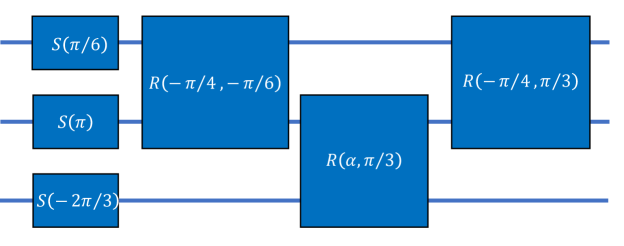
Figure 4: Quantum circuit realizing the $3$-qubit fermionic Fourier transform $\mathsf{F}$. The circuit was generated using Algorithm 1. Here $\alpha=-(1/2)\arccos{(1/3)}\approx-0.9553$.

Appendix B

Here we prove Lemma 7. First note that

$$\mathsf{C}=\mathsf{SWAP}_{0,1}\mathsf{SWAP}_{1,2}\cdots\mathsf{SWAP}_{n-2,n-1}.$$

Define a fermionic SWAP operator [18, 23]

$$\mathsf{fSWAP}=\mathsf{CZ}\cdot\mathsf{SWAP}=\left[\begin{array}[]{cccc}1&0&0&0\\ 0&0&1&0\\ 0&1&0&0\\ 0&0&0&-1\\ \end{array}\right]$$ (27)

and a fermionic cyclic shift

$$\mathsf{fC}=\mathsf{fSWAP}_{0,1}\mathsf{fSWAP}_{1,2}\cdots\mathsf{fSWAP}_{n-2,n-1}.$$ (28)

A simple algebra shows that

$$\mathsf{C}|x\rangle=(-1)^{x_{n-1}(x_{0}+x_{1}+\ldots+x_{n-2})}\mathsf{fC}|x\rangle.$$ (29)

Let $k=x_{0}+x_{1}+\ldots+x_{n-1}$ be the Hamming weight of $x$. Then

$$(-1)^{x_{n-1}(x_{0}+x_{1}+\ldots+x_{n-2})}=(-1)^{x_{n-1}(k-x_{n-1})}=(-1)^{x_{n-1}k+x_{n-1}}=(-1)^{x_{n-1}(k+1)}.$$ (30)

Thus $\mathsf{C}\,{=}\,\mathsf{fC}$ on the odd-weight subspace and $\mathsf{C}\,{=}\,\mathsf{fC}Z_{n-1}$ on the even-weight subspace, i.e.

$$\mathsf{C}=E\mathsf{fC}Z_{n-1}+(I-E)\mathsf{fC}.$$ (31)

We claim that

$$\mathsf{fC}=\mathsf{F}e^{iH_{0}}\mathsf{F}^{\dagger}.$$ (32)

Indeed, let

$$G\equiv\mathsf{F}e^{iH_{0}}\mathsf{F}^{\dagger}.$$

First note that $\mathsf{fC}|0^{n}\rangle=G|0^{n}\rangle=|0^{n}\rangle$. Since any state can be obtained from $|0^{n}\rangle$ by applying the creation operators $a_{p}^{\dagger}$, it suffices to check that

$$\mathsf{fC}^{\dagger}a_{p}\mathsf{fC}=G^{\dagger}a_{p}G$$

for all $p$. A simple algebra shows that

$$(\mathsf{fSWAP}_{p,p+1})a_{p}(\mathsf{fSWAP}_{p,p+1})^{\dagger}=a_{p+1}\quad\mbox{and}\quad(\mathsf{fSWAP}_{p,p+1})a_{p+1}(\mathsf{fSWAP}_{p,p+1})^{\dagger}=a_{p}.$$

Combining this and Eq. (28) one gets

$$\mathsf{fC}^{\dagger}a_{p}\mathsf{fC}=a_{p-1},$$

where the indices of fermionic operators are evaluated modulo $n$. Using the identities

$$e^{-iH_{0}}a_{q}e^{iH_{0}}=e^{2\pi iq/n}a_{q},$$

$$\mathsf{F}a_{p}\mathsf{F}^{\dagger}=\frac{1}{\sqrt{n}}\sum_{q\in\mathbb{Z}_{n}}^{n}e^{2\pi ipq/n}a_{q},\quad\mbox{and}\quad\mathsf{F}^{\dagger}a_{q}\mathsf{F}=\frac{1}{\sqrt{n}}\sum_{r\in\mathbb{Z}_{n}}^{n}e^{-2\pi iqr/n}a_{r},$$

one gets

$$G^{\dagger}a_{p}G=n^{-1/2}\sum_{q\in\mathbb{Z}_{n}}e^{2\pi i(1-p)q/n}\mathsf{F}a_{q}\mathsf{F}^{\dagger}=n^{-1}\sum_{q,r\in\mathbb{Z}_{n}}e^{2\pi i(1-p+r)q/n}a_{r}=a_{p-1}.$$

Thus $G^{\dagger}a_{p}G=\mathsf{fC}^{\dagger}a_{p}\mathsf{fC}=a_{p-1}$, proving Eq. (32).

Next we claim that

$$\mathsf{fC}Z_{n-1}=e^{-iH_{0}/2}\mathsf{fC}e^{iH_{0}/2}e^{i(\pi/n)W}.$$ (33)

Indeed, let

$$L:=\mathsf{fC}Z_{n-1}\quad\mbox{and}\quad R:=e^{-iH_{0}/2}\mathsf{fC}e^{iH_{0}/2}e^{i(\pi/n)W}.$$

Since $L|0^{n}\rangle=R|0^{n}\rangle=|0^{n}\rangle$, it suffices to check that $L^{\dagger}a_{p}L=R^{\dagger}a_{p}R$ for all $p\in\mathbb{Z}_{n}$. A simple algebra gives

$$e^{-i(\pi/n)W}a_{p}e^{i(\pi/n)W}=e^{i(\pi/n)}a_{p},$$

$$Z_{n-1}a_{p}Z_{n-1}=\left\{\begin{array}[]{rcl}a_{p}&\mbox{if}&0\leq p\leq n-2\\ -a_{p}&\mbox{if}&p=n-1\\ \end{array}\right.,$$

$$e^{iH_{0}/2}a_{p}e^{-iH_{0}/2}=e^{-i\pi p/n}a_{p},\quad\mbox{and}\quad e^{-iH_{0}/2}a_{p}e^{iH_{0}/2}=e^{i\pi p/n}a_{p}$$

for all $p\in\mathbb{Z}_{n}$. Recall that $\mathsf{fC}^{\dagger}a_{p}\mathsf{fC}=a_{p-1}$. Using the above identities one gets

$$L^{\dagger}a_{p}L=\left\{\begin{array}[]{rcl}a_{p}&\mbox{if}&1\leq p\leq n-1\\ -a_{p}&\mbox{if}&p=0\\ \end{array}\right.$$

and

$$R^{\dagger}a_{p}R=e^{-i\pi p/n}e^{i\pi p^{\prime}/n}e^{i(\pi/n)}a_{p-1},$$

where $p^{\prime}\equiv p-1{\pmod{n}}$. Note that

$$e^{-i\pi p/n}e^{i\pi p^{\prime}/n}=\left\{\begin{array}[]{rcl}e^{-i\pi/n}&\mbox{if}&1\leq p\leq n-1\\ -e^{-i\pi/n}&\mbox{if}&p=0\\ \end{array}\right..$$

Thus $L^{\dagger}a_{p}L=R^{\dagger}a_{p}R$, that is, $L{=}R$, proving Eq. (33).

Combining Eqs. (31,32,33) one infers that the restrictions of $\mathsf{C}$ onto the odd-weight and even-weight subspaces coincide with the operators

$$\mathsf{C}_{odd}=\mathsf{F}e^{iH_{0}}\mathsf{F}^{\dagger}$$

and

$$\mathsf{C}_{even}=e^{-iH_{0}/2}(\mathsf{F}e^{iH_{0}}\mathsf{F}^{\dagger})e^{iH_{0}/2}e^{i(\pi/n)W}$$

respectively. Thus

$$\mathsf{C}=e^{-iH_{0}E/2}(\mathsf{F}e^{iH_{0}}\mathsf{F}^{\dagger})e^{iH_{0}E/2}e^{i(\pi/n)WE}$$

on the full Hilbert space. Recall that the fermionic Fourier transform $\mathsf{F}$ preserves the Hamming weight. Thus $\mathsf{F}^{\dagger}$ commutes with $e^{i(\pi/n)WE}$. Commuting the term $e^{i(\pi/n)WE}$ to the left gives

$$\mathsf{C}=e^{-iH_{0}E/2}\mathsf{F}\left(e^{iH_{0}}e^{i(\pi/n)WE}\right)\mathsf{F}^{\dagger}e^{iH_{0}E/2}=V^{\dagger}e^{iH^{\prime}}V,$$

where $V=\mathsf{F}^{\dagger}e^{iH_{0}E/2}$ and $H^{\prime}=H_{0}+(\pi/n)WE$. Thus $\mathsf{C}=e^{iV^{\dagger}H^{\prime}V}$, proving Lemma 7.

References

[1]
Randal E. Bryant.
Graph-based algorithms for Boolean function manipulation.
IEEE Transactions on Computers, 100(8):677–691, 1986.
[2]
Christoph Meinel and Thorsten Theobald.
Algorithms and Data Structures in VLSI Design: OBDD-foundations
and applications.
Springer Science & Business Media, 2012.
[3]
Randal E. Bryant.
On the complexity of VLSI implementations and graph representations
of Boolean functions with application to integer multiplication.
IEEE Transactions on Computers, (2):205–213, 1991.
[4]
Beate Bollig, Martin Löbbing, Martin Sauerhoff, and Ingo Wegener.
On the complexity of the hidden weighted bit function for various
BDD models.
RAIRO-Theoretical Informatics and Applications, 33(2):103–115,
1999.
[5]
Dmitri Maslov, Gerhard W. Dueck, and D. Michael Miller.
Toffoli network synthesis with templates.
IEEE Transactions on Computer-Aided Design of Integrated
Circuits and Systems, 24(6):807–817, 2005.
[6]
Aditya K. Prasad, Vivek V. Shende, Igor L. Markov, John P. Hayes, and Ketan N.
Patel.
Data structures and algorithms for simplifying reversible circuits.
ACM Journal on Emerging Technologies in Computing Systems
(JETC), 2(4):277–293, 2006.
[7]
Dmitri Maslov, Gerhard W. Dueck, and D. Michael Miller.
Techniques for the synthesis of reversible Toffoli networks.
ACM Transactions on Design Automation of Electronic Systems
(TODAES), 12(4):42.1–28, 2007.
[8]
James Donald and Niraj K. Jha.
Reversible logic synthesis with Fredkin and Peres gates.
ACM Journal on Emerging Technologies in Computing Systems
(JETC), 4(1):1–19, 2008.
[9]
Mehdi Saeedi, Morteza Saheb Zamani, Mehdi Sedighi, and Zahra Sasanian.
Reversible circuit synthesis using a cycle-based approach.
ACM Journal on Emerging Technologies in Computing Systems
(JETC), 6(4):1–26, 2010.
[10]
Dmitri Maslov, Gerhard W. Dueck, and D. Michael Miller.
Synthesis of Fredkin-Toffoli reversible networks.
IEEE Transactions on Very Large Scale Integration (VLSI)
Systems, 13(6):765–769, 2005.
[11]
Mehdi Saeedi and Igor L. Markov.
Synthesis and optimization of reversible circuits—a survey.
ACM Computing Surveys (CSUR), 45(2):1–34, 2013.
[12]
Dmitry V. Zakablukov.
Application of permutation group theory in reversible logic
synthesis.
arXiv:1507.04309, 2015.
[13]
Vivek V. Shende, Stephen S. Bullock, and Igor L. Markov.
Synthesis of quantum-logic circuits.
IEEE Transactions on Computer-Aided Design of Integrated
Circuits and Systems, 25(6):1000–1010, 2006.
[14]
Dmitri Maslov.
Reversible logic synthesis benchmarks page.
https://webhome.cs.uvic.ca/~dmaslov/hwbpoly.html, 2005.
[15]
David A. Barrington.
Bounded-width polynomial-size branching programs recognize exactly
those languages in NC1.
Journal of Computer and System Sciences, 38(1):150–164, 1989.
[16]
Farid Ablayev, Aida Gainutdinova, Marek Karpinski, Cristopher Moore, and
Christopher Pollett.
On the computational power of probabilistic and quantum branching
program.
Information and Computation, 203(2):145–162, 2005.
[17]
Ryan Babbush, Nathan Wiebe, Jarrod McClean, James McClain, Hartmut Neven, and
Garnet Kin Chan.
Low depth quantum simulation of electronic structure.
Physical Review X, 8:011044, 2018.
[18]
Ian D. Kivlichan, Jarrod McClean, Nathan Wiebe, Craig Gidney, Alán
Aspuru-Guzik, Garnet Kin-Lic Chan, and Ryan Babbush.
Quantum simulation of electronic structure with linear depth and
connectivity.
Physical Review Letters, 120(11):110501, 2018.
[19]
Algirdas Avizienis.
Signed-digit number representations for fast parallel arithmetic.
IRE Transactions on Electronic Computers, (3):389–400, 1961.
[20]
Ingo Wegener.
The complexity of Boolean functions.
BG Teubner, 1987.
[21]
Valerii M. Krapchenko.
Asymptotic estimation of addition time of parallel adder.
Syst. Theory Res., 19:105–122, 1970.
[22]
Michael A. Nielsen and Isaac Chuang.
Quantum computation and quantum information, 2002.
[23]
Frank Verstraete, J. Ignacio Cirac, and José I. Latorre.
Quantum circuits for strongly correlated quantum systems.
Physical Review A, 79(3):032316, 2009.