Information Freshness of Updates Sent over LEO Satellite Multi-Hop Networks

Abstract

Low Earth Orbit (LEO) satellite constellations are bringing the Internet of Things (IoT) to the space arena, also known as non-terrestrial networks. Several IoT satellite applications for tracking ships and cargo can be seen as exemplary cases of intermittent transmission of updates whose main performance parameter is the information freshness. This paper analyzes the Age of Information (AoI) of a satellite network with multiple sources and destinations that are very distant and therefore require several consecutive multi-hop transmissions. A packet erasure channel and different queueing policies are considered. We provide closed-form bounds and tight approximations of the average AoI, as well as an upper bound of the Peak Age of Information (PAoI) distribution as a worst-case metric for the system design. The performance evaluation reveals complex trade-offs among age, load, and packet losses. The optimal operational point is found when the combination of arrival rates and packet losses is such that the system load can ensure fresh information at the receiver; nevertheless, achieving this is highly dependent on the mesh topology. Moreover, the potential of an age-aware scheduling strategy is investigated and the fairness among users discussed. The results show the need to identify the bottleneck nodes for the age, as improving the rate and reliability of those critical links will highly impact on the overall performance. The model is general enough to represent other multi-hop mesh networks.

I Introduction

Satellite communications are characterized by the inherent delay due to the large physical distances. Such propagation delay is highly reduced when using Low Earth Orbit (LEO) satellites with altitudes between 500 and 2000 km, and propagation delays in the order of milliseconds. Unlike geostationary orbits, LEO satellites move fast with respect to the Earth’s surface and have a small ground coverage: only 0.45 % of the Earth’s surface for a LEO satellite deployed at 600 km and with an elevation angle of 30 degrees. To ensure that any ground terminal is always covered by, at least, one satellite, a flying formation of many satellites is required, usually organized in a constellation with coordinated ground coverage [1, 2].

Latency-sensitive information might suffer from long delays even with low orbits, because several inter-connected satellites are required to connect two distant points on the Earth’s surface. The result is a multi-hop network where intermediate nodes (satellites) along the path receive and forward packets via wireless links. The introduction of multi-hop connectivity has the drawback of additional latency [3, 4], as the total latency is a combination of processing delay, queueing delay, transmission time and propagation delay at each hop.

Besides latency, a related quantity of interest that has recently attracted significant information is the Age of Information (AoI) metric [5]. AoI is defined as the time elapsed since the last received message containing update information was generated and it can be interpreted as a representative of the freshness of the sensory information at the receiver. Many Internet of Things (IoT) applications that rely on satellites involve tracking of e.g. ships or cargo, such that an IoT transmission in this setting is often a real-time status update. Hence, satellite IoT communication entails some of the exemplary cases where information freshness and AoI are of primary importance, rather than the conventional latency or packet delay. These examples include the recently-introduced VHF Data Exchange System (VDES) [6][7] for maritime communications and its predecessor Authentication Identification System (AIS). The Peak Age of Information (PAoI) [8] is a byproduct of the age process that quantifies the worst case.

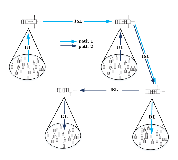
Figure 1: Example of a multi-hop relaying satellite network with multiple sources and destinations. There are a total of four nodes and two exemplary path routes indicated in light blue and dark blue.

In this paper, we address a general buffer-aided multi-hop network with multiple sources and destinations. We focus on applications where a number of mutually independent traffic sources need to report sensory updates to a number of control stations in a timely fashion, and do so through a chain of LEO satellites. Since the end-points are too far to be linked by a single connection, several satellites connected by Inter-Satellite Links (ISLs) are required to relay the information to the final point.

As Fig. 1 shows, all the satellites work as a relay and, at the same time, receive uplink status-updates from their coverage area and are the final destination for some of the status-updates. At each satellite, the ISL is used to forward both the ground information from satellite and the packets from neighboring satellites. Different sources can have partly overlapping paths, using the same relays for part of their connection to their ground destinations, which can be ground stations, gateways, or ground devices with direct connectivity to the satellite network. The ISL links, the uplink from the source to the first satellite, and the downlink from the last satellite to the ground destination can have different capacities and packet loss rates, due to the different technologies, propagation environments, and power budgets [2, 9].

These multi-hop networks are difficult to study theoretically due to the complex interactions between subsequent queueing systems, and the literature on the subject is limited. In this queueing network, the server represents the wireless links whose rates are different, and each node works as a relay for the previous node and receives data packets from its directly connected traffic source. These two main traits of the model greatly complicate the queueing system. Furthermore, the presence of errors in the transmission of packets and the policy to select the next packet in each queue add another layer of complexity to the determination of the AoI. To the best of our knowledge, this is the first work to get a very good approximation and upper and lower bounds on the average AoI and the total delay for general network topologies. Moreover, we also derive an upper bound on the tail of the PAoI, which is critical for worst-case performance analysis.

The rest of the paper is organized as follows: Sec. II presents an overview of related work and the main contributions. Then, Sec. III describes the system model and the analytical tools to tackle the problem. Sec. IV presents the AoI analysis for the general $K$-node case, with tight higher and lower bounds, while we derive an upper bound on the distribution tail in Sec. IV-C. Numerical results are presented in Sec. V. Finally, Sec. VI discusses the conclusions and future directions of this work.

II Related work and contributions

Latency has been widely studied in the context of satellite communications, from Geo-synchronous Equatorial Orbit (GEO) to LEO orbits. However, the metric of interest has historically been the end-to-end (E2E) latency, defined as the time it takes a bit of information to traverse a network from its originating point to its final destination. Indeed, the E2E delay performance was already investigated more than twenty years ago [10, 11] for a LEO satellite-ATM network. More recently, [12] proposes a method for obtaining the E2E latency in satellite IP-based networks and it is found that for GEO at least 50% of the E2E latency is due to the processing and transmission times. A tandem queue similar to ours is used in [13] to model a multi-layered satellite network combining LEO and Medium Earth Orbit (MEO). Specifically, stochastic network calculus is used to obtain the E2E delay and backlog bounds. The problem of stochastic network calculus is, however, that the bounds can be very loose [14]. The author in [15] investigates the potential of one of the imminent commercial constellations, Starlink, to provide low-latency. In [16] a satellite relay network is considered, and Machine Learning (ML)-based protocols for Delay Tolerant Networking are discussed. To the best of our knowledge, our previous paper [17] was the first one addressing AoI in a satellite set-up with inter-connected nodes, and in that prior work we provided initial results of the age in a multi-hop line system with ideal transmissions and First Come First Serve (FCFS) policy.

As already mentioned, age-sensitive applications are those where a source generates updates that are transmitted through a communication network, like common satellite services that involve tracking processes or objects such as containers in logistics. The previously mentioned VDES [6][7] and AIS are meant to allow vessels to periodically report their position, course and speed, for collision avoidance, but the small assigned bandwidth makes the system design and the performance guarantee highly challenging. Another example is the Automatic Dependent Surveillance - Broadcast (ADS-B) system in airplanes [18], where maintaining fresh information on the sender’s status is the first and foremost objective of the network.

The AoI metric has been extensively studied in several different queueing systems: the original paper that defined it [5] analyzed the $G/G/1$ queue, concentrating on the exponential and deterministic distributions as case studies. Later works tried to calculate the AoI and PAoI in specific realistic models of wireless channels, including errors [19] and retransmissions [20] and verifying the queueing models with live experiments [21]. An interesting addition to the model is the consideration of multiple sources, which leads to a scheduling problem with the objective of limiting the age for each source [22] focused on the optimal scheduling protocols to improve the freshness of information in wireless networks. Optimizing the senders’ updating policies in complex wireless communication systems has been proven to be an NP-hard problem, but near-optimal solutions can be achieved using greedy heuristics [23] such as “lazy updates”: each source can decide not to send some packet, waiting for new information to avoid overloading the queue with packets that give a limited benefit to the overall AoI [24]. Another possibility is to consider a limited transmission window for packets, after which they are dropped: in [25], the average PAoI is derived in such a scenario. Closed form expressions for the average AoI of slotted and unslotted ALOHA have been given in [26] and [27]. The metric has been compared to the performance of scheduled multiple access in [28]. Some selective packet transmission policies at source have been considered in [29], an optimal AoI of a stabilized slotted ALOHA can be approximated by $1/N\lambda_{0}$ where $N\lambda_{0}$ is the sum arrival rate from N sources of updates if $N\rightarrow\infty$ and $N\lambda_{0}<1/e$.

If the connection is not single-hop, and there are several queueing systems in sequence, the network can be modeled as a tandem queue. Given the wide range of relevant applications, we focus our attention in the study of the age in this kind of models, which is particularly interesting in satellite relay applications, as LEO, but also the other, satellite networks are inherently multi-hop. If a single satellite relay is employed, the model is a 2-hop tandem queue, for which the average PAoI under FCFS queueing was derived in [30] for the multiple source case under $M/M/1$ systems. The Chernoff bound can be used to get an upper bound of the Cumulative Density Function (CDF) of the AoI in these kinds of systems [31], while our recent work [32] derives the distribution analytically.

A general result was proven for queueing networks with any number of systems in [33] and  [34]: in any tandem of $M/M/1$ systems with a single source, the AoI is minimized by applying the preemptive Last Come First Serve (LCFS) policy. A more general result was derived in [35], in which the authors study AoI in a general multi-source multi-hop wireless network with explicit channel contention and have obtained upper and lower bounds for the average AoI and PAoI based on fundamental graph parameters such as the connected domination number and average shortest path length. In [36], the problem of multi-hop networks with many source-destination pairs and interference constraints is addressed, and the optimal policy is reduced to solving the equivalent problem in which all source-destination pairs are just a single-hop away. Queueing is a major source of delay, and updates do not need to be transmitted reliably, so it is often better to drop the packet in service and transmit the freshest one directly. A similar result has been proven for $M/M/k$ queues [37], and [38] derives the average AoI with preemption for 2-hop systems with different arrival processes. The problem is more interesting for different service time distributions, as the decision over whether to preempt or not becomes more complex [39]. An analysis of the effect of preemption on tandem models on the average AoI is presented in [40]: the work extends the stochastic hybrid system analysis, generalizing it for the moment generation function of the ageing process for a class of queueing networks with preemptive services and memoryless service times. Another possibility is queue replacement, in which only the freshest update for each source is kept in the queue, reducing queue size significantly: the replaced packet is not placed in the queue, but dropped altogether, reducing channel usage with respect to simple LCFS, with or without preemption. In this case, the queue is modeled as an $M/M/1/2$, and if a new packet arrives it takes the queued packet’s place. Some preliminary results on such a system are given in [41], while the average AoI and PAoI are computed in [42] for one source and in [43] for multiple sources. Finally, a general transport protocol to control the generation rate of status updates to minimize the AoI over the Internet is presented in [44].

Our work considers a general queueing network with $K$ nodes and multiple sources and destinations, on which very little work has been done. Specifically, the main contributions of the paper are:

• We model a satellite relay system as a multi-hop mesh network with packet losses and multiple sources and destinations. Each node $k$ receives traffic from multiple sources and forwards it to other satellites through the ISL, or to its destination through the downlink. This very general model is meant to represent satellite relay systems, but it can be applied to other multi-hop ad hoc networks with multiple relays and multiple sink nodes, independently of their topology. An initial version of this model was presented in [17], which analyzed a simple tandem queue with 2 satellite nodes. In this work, the model is fully general, and can represent any network with Poisson traffic and service, with arbitrary error rates for each link.

• We provide novel analytical results of the AoI in this scenario: (1) a tight approximation and higher and lower bounds of the average AoI; (2) an upper bound of the PAoI distribution; (3) and the exact value of the mean system delay. We show the results for a line network in which all sources have the same sink, and in a traditional dumbbell topology in which multiple connections share a single ISL link. The analysis is done for infinite buffers at each node, but it has been observed that having a limited storage capacity has little impact in the age performance of the multi-hop network.

• We investigate user fairness and the impact of age-aware scheduling policies through the analysis of three queueing policies: FCFS, Oldest Packet First (OPF) and Highest Age First (HAF). The conventional FCFS is a scheduling strategy well-suited for single queues, but it does not take into account the multi-hop nature of the network. Instead, our results show that the OPF and HAF policies, especially OPF, are able to increase the fairness between sources in different parts of the network while maintaining a similar average AoI.

• We analyze the presence of wireless channel errors and their impact in the AoI. A packet erasure channel models the losses in the wireless links. Lost packets are detrimental for the packet delay performance but, interestingly, the AoI benefits from the load reduction of packet dropping when the system works close to congestion. This trade-off is yet another instance of the age-dilemma “how often should one update?” [5], although the answer in a system with multiple sources and multiple destinations is not trivial.

III System model

We consider a connection composed of $K$ links in a multi-hop mesh network in which each node in the network acts both as a source and a relay, as shown in Fig. 1. The source is modeled as a Poisson process, generating packets with rate $\lambda$. Each node $k$ in the connection, including the source, receives Poisson cross traffic with rate $\theta_{k}$. Cross traffic might share part of the path with the packets from the source, and this is accounted for by the parameter $\psi_{k}$: a fraction $\psi_{k}$ of the cross traffic entering node $k$ leaves the connection, as it is transmitted through another link to nodes outside the considered source’s path; the rest of the traffic is transmitted through the same path as the considered source’s packets. In any case, the destination is on ground, for which the last node in the source’s path represents the downlink (DL). We assume that each satellite can receive and transmit packets at the same time over different ISLs. The ISL connects satellites in the same orbital plane or in different orbital planes, for which dedicated antennas are typically located in the roll and pitch axes, respectively. Moreover, the DL has another dedicated antenna pointing at the Earth’s center. If the information from the source is delay-sensitive (e.g., status updates), it must be routed as soon as possible to the destination, and AoI is a useful metric for system performance.

We model a connection between a source and a destination as an $M/M/1$ queueing network connected in series. In a real system, the service time for each link depends on the length of the packet and the quality of the link: in this work, we model the service time for each link for the same packet as independent for tractability. This assumption is equivalent to considering uncorrelated distances between pairs of satellites; considering a correlated system is left for future work. Each node $k$ receives traffic from the node, as well as cross traffic, some of which is then routed through other connections or arrives at its destination. This model is fully general, as it can describe any network with Poisson sources, from the point of view of any of the traffic flows in the network. We model the $k$-th link in the connection, between nodes $k$ and $k+1$, as an erasure channel with an error probability $\varepsilon_{k}$: any packet sent by node $k$ is correctly received by node $k+1$ with probability $1-\varepsilon_{k}$. The service follows a Poisson process with rate $\mu_{k}$, i.e., the average service time of each link is the inverse of the service rate, $S_{k}=1/\mu_{k}$. This model is general enough to capture heterogeneous capabilities and losses in a satellite network, where the links (ISL in the same orbital plane or between different planes, and the DL) can be of a highly different nature. The system can be entirely described by the source rate $\lambda$ and the vectors $\bm{\theta}$, $\bm{\psi}$, $\bm{\mu}$, and $\bm{\varepsilon}$, which describe the cross traffic and the channels’ statistical properties. Using these vectors, we can compute the total cross traffic load at node $k$, denoted as $\bar{\theta}_{k}$:

$$\bar{\theta}_{k}=\sum_{j=1}^{k}\theta_{j}\prod_{i=j}^{k-1}(1-\psi_{i})(1-\varepsilon_{i}).$$ (1)

As Fig. 2 shows, each node in the connection receives traffic from the previous node, as well as cross traffic: a part of the cross traffic leaves the connection, as it is transmitted through other paths, while the rest is transmitted along the connection with the considered source’s packets.

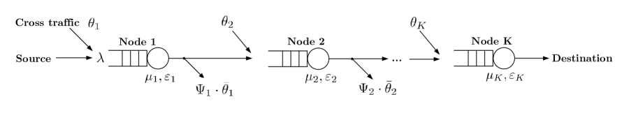
Figure 2: General multi-hop queueing system with cross traffic.

The arrival process at the source node models the uplink (UL) access in the satellite network. This access can be implemented in many different ways. For a large number of intermittent transmitters in a single shared communication channel, the ALOHA protocol is the simplest one and it is widely used [45]. Rather than the conventional ALOHA implementation with a backoff mechanism to re-send colliding packets, a pure ALOHA scheme with a single transmission attempt is more suitable for age-sensitive applications. Thus, the source transmits each new available status update immediately and a collision occurs when other users transmit their packets simultaneously. We can consider two extreme cases in this part of the model:

• Ideal Multi-Packet Reception (MPR). In this case [46] the packets are not lost due to collisions and can only be lost due to channel errors. This model is suitable for IoT systems based on Ultra-Narrowband (UNB) transmissions, such as SigFox [47], where the receiver is designed to take advantage of the very small bandwidth occupied by a single packet and decode multiple packets simultaneously.

• Destructive collisions. The other extreme is adoption of the classical ALOHA model, in which any collision is destructive and all packets involved in the collision are lost. Strictly speaking, here the resulting process is not Poisson due to the correlation created when multiple packets are lost in a collision create.

Regardless of whether we model losses as destructive collisions or channel errors, the failed sources will not try again, but just wait until the next status update is generated, and $p_{c}$ is the probability of incorrect packet decoding due to either channel error or collision. In case of MPR, the arrival process of the packets that reach the first satellite is still Poisson, but thinned with probability $(1-p_{c})$, such that the resulting arrival rate is $\lambda(1-p_{c})$. In case of destructive collisions, the error source is both channel noise and collision. For this case the thinned Poisson process with arrival rate $\lambda(1-p_{c})$ is only an approximation. As shown in Fig. 3, where we compare the ALOHA departure process with arrival rate $\lambda_{a}$ and a Poisson arrival process with rate $\lambda_{p}=\lambda_{a}(1-p_{c})$, the approximation is justified for a wide range of arrival rates. This will be verified in the overall results as well.

Figure 3: CDF of the interdeparture time.

With this model, the difference between the age before the access and the age at the queue of the first satellite is just a constant delay corresponding to the UL transmission time. We denote the AoI in the destination node at time $t$ as the random process $\Delta(t)$, which increases linearly in time in the absence of any updates, and is reset to a smaller value when an update is received. For the reader’s convenience the complete list of notations is given in Table I. In addition, for a random variable (RV) $X$, $\mathbb{E}[X]$ stands for the expected value and $f_{X}(x)$ denotes Probability Distribution Function (PDF) of $X$.

Note that, if we use the standard FCFS policy, traffic from all sources is stored in the same buffer, with no priorities among them. We will later analyze the case in which nodes apply the OPF and HAF queueing policies. OPF prioritizes packets by their generation time instead of their arrival time at the node, enhancing fairness between different flows, as packets that have already gone through longer connections can traverse later links faster, at the expense of fresher packets from sources closer to their destination. Differently, HAF is not aimed at fairness, but at improving AoI, as it prioritizes packets whose source has the highest current AoI at the node.

TABLE I: Relevant notation

Notation	Definition	Notation	Definition
$K$	Number of links in a multi-hop network	$N(\mathcal{T})$	Number of arrivals from source by time $\mathcal{T}$
$\lambda$	Packets generation rate at source	$\Delta_{\mathcal{T}}$	Time average AoI over $\mathcal{T}$
$\theta_{k}$	cross traffic rate at node $k$	$\bar{\Delta}$	Average AoI
$\bar{\theta}_{k}$	Total cross traffic load at node $k$	$\rho_{k}$	Traffic load at node $k$
$\bm{\theta}$	Vector of cross traffic rates	$\rho$	Error free load
$\psi_{k}$	Probability of cross traffic offloading in $k$	$S_{k}$	Average service time at node $k$
$\bm{\psi}$	Vector of cross traffic offloading probabilities	$\Delta(t)$	Ageing process
$p_{s}(j)$	Packet delivery success probability over $j$ links	$\xi_{i}$	PAoI of packet $i$
$\varepsilon_{k}$	Channel error probability for the $k$-th link	$\alpha_{k}$	Packets response rate at node $k$
$\bm{\varepsilon}$	Vector of channel error probabilities	$\bm{\alpha}$	Vector of response rates
$\mu_{k}$	Packet service rate at node $k$	$t_{i}$	Status update $i$ generation time (by source)
$\bm{\mu}$	Vector of service rates	$t^{\prime}_{i}$	Status update $i$ time at monitor (on ground)
$\delta_{ij}$	Hypoexponential distribution coefficient of packet service time	$\Pi_{j}(n)$	Steady-state distribution of the number of queued packets at node $j$
$\gamma_{ij}$	Hypoexponential distribution coefficient of packet total network time	$\bm{\omega}$	Vector of hypoexponentional distribution parameters for the PAoI bound
$Y_{i}$	Packet interarrival time	$p_{c}$	Uplink collision probability
$Z_{i}$	Packet interdeparture time	$Q_{i}$	Area under the $\Delta(t)$ AoI process
$T_{i}$	Packet $i$ network time	$Q^{\prime}_{i}$	Additional area below the $\Delta(t)$ process after a
$T_{i,j}$	Packet $i$ system time at node $j$		missed packet
$W_{i}$	Packet $i$ total waiting time	$Q^{(n)}_{i}$	Total area around $\Delta(t)$ process after $n$ missed
$W_{i,j}$	Packet $i$ waiting time at node $j$		packets
$S_{i}$	Packet $i$ total service time	$\Omega_{j}$	Time difference between arrival and departure
$S_{i,j}$	Packet service time at node $j$		time of two consecutive packets at node $j$

III-A Average AoI in the error-free scenario

Figure 4: Evolution of the Age of Information in a queue network with $K$ nodes. The network times $T_{i}$ are defined as the total time spent in the system, since arrival in node $1$ until departure in node $K$.

We first consider an error-free scenario, in which $\varepsilon_{k}=0\;\forall k$. In this case, the evolution of the AoI $\Delta(t)$ for source under a FCFS policy exhibits the sawtooth pattern plotted in Fig. 4. Without loss of generality, the system is first observed at $t=0$ and the queue is empty with age $\Delta(0)$. The status update $i$ is generated at time $t_{i}$ and is received by the ground station at time $t_{i}^{\prime}$. We define $Y_{i}$ as the interarrival time $Y_{i}=t_{i}-t_{i-1}$ between two packets, $Z_{i}$ as the interdeparture time $Z_{i}=t^{\prime}_{i}-t^{\prime}_{i-1}$, and $T_{i}$ as the total network time in the system $T_{i}=t^{\prime}_{i}-t_{i}$. The latter includes the time spent in all the nodes (queueing time and transmission time) until departure from the system at node $K$. Our definitions follow the work in [48], which considered a single buffered system, but in our case, the E2E connection is modeled as a sequence of $M/M/1$ systems, each of which has to deal with cross traffic.

To evaluate the average AoI, the strategy is to calculate the area under $\Delta(t)$, or the time average AoI, as

$$\Delta_{\mathcal{T}}=\frac{1}{\mathcal{T}}\left(Q_{\text{ini}}+Q_{\text{last}}+\sum_{i=2}^{N(\mathcal{T})}Q_{i}\right),$$ (2)

where $N(\mathcal{T})$ is the number of arrivals from the source by time $\mathcal{T}$. The average AoI $\bar{\Delta}$ is given by the limit $\bar{\Delta}=\lim_{\mathcal{T}\rightarrow\infty}\Delta_{\mathcal{T}}$. As defined in Fig. 4, each $Q_{i}$ (with $i>1$) is a trapezoid whose area can be calculated as the difference between two isosceles triangles [48], i.e.,

$$Q_{i}=\frac{1}{2}\left(T_{i}+Y_{i}\right)^{2}-\frac{1}{2}T_{i}^{2}=Y_{i}T_{i}+\frac{Y_{i}^{2}}{2}.$$ (3)

The average AoI $\bar{\Delta}$ can then be expressed as

$$\bar{\Delta} =\lambda\mathbb{E}\left[Q_{i}\right]=\lambda\left(\mathbb{E}\left[T_{i}Y_{i}\right]+\mathbb{E}\left[\frac{1}{2}Y_{i}^{2}\right]\right)^{\prime}.$$ (4)

Ergodicity has been assumed for the stochastic process $\Delta(t)$, but no assumptions regarding the distribution of the random variables $Y$ and $T$ have been made. Considering that the arrival process is Poisson, the interarrival times $Y_{i}$ are exponentially distributed with rate $\lambda$. The second term in (4), $\mathbb{E}\left[\frac{1}{2}Y_{i}^{2}\right]$, is then easily obtained as $\mathbb{E}\left[\frac{1}{2}Y_{i}^{2}\right]=\frac{1}{\lambda^{2}}$. The other term in (4) is harder to derive, as $T_{i}$ is correlated to $Y_{i}$. Intuitively, a packet coming right after another packet from the same source will experience a higher queueing delay, while a packet that arrives a long time after the previous one from the same source will just have to deal with the cross traffic, as all packets from the source will have already been transmitted.

III-B Average AoI in the error-prone scenario

Figure 5: Evolution of the Age of information in a queue network with $K$ nodes and errors. The additional area $Q^{\prime}_{2}$, highlighted in red, shows the increase in the AoI in case a packet is lost.

We now consider the more general case with transmission errors: we assume that each link $j$ has a known error probability $\varepsilon_{j}$, and that a lost packet has the same service time as a correctly received packet, but is not put in the queue for the next node. Fig. 5 shows the geometric analysis for the evolution of the AoI for a specific source in case of errors: if packet 2 is dropped, the additional area $Q^{\prime}_{2}$, highlighted in red in the figure, needs to be included in the computation. If we consider the $Q^{(1)}_{i}=Q_{i}+Q_{i-1}+Q^{\prime}_{i-1}$ trapezoid resulting from a single lost packet, its area is given by:

$$Q^{(1)}_{i}=\frac{1}{2}\left(T_{i}+Y_{i}+Y_{i-1}\right)^{2}-\frac{1}{2}T_{i}^{2}=Y_{i}T_{i}+Y_{i-1}T_{i}+\frac{Y_{i}^{2}}{2}+\frac{Y_{i-1}^{2}}{2}.$$ (5)

The trapezoid is the sum of the red and yellow areas in the figure. We can generalize this result to the case with $n$ errors:

$$Q^{(n)}_{i} =\sum_{j=0}^{n}\left[Y_{i-j}T_{i}+\frac{1}{2}Y_{i-j}^{2}\right]+\sum_{j=0}^{n}\sum_{\ell=0,\ell\neq j}^{n}Y_{i-j}Y_{i-\ell}$$ (6)

We note here that, since each node is an $M/M/1$ queue, the interarrival times $Y_{i}$ and $Y_{i-j}$ are independent for any $j>0$, and so are $T_{i}$ and $Y_{i-j}$. When the system reaches a steady state, the system times are stochastically identical, i.e., $T=^{st}T_{i}=^{st}T_{i-1}$, and the same holds for the interarrival times. Since errors are assumed to be independent, and the probability of delivering a packet through the first $j$ links correctly is $p_{s}(j)=\prod_{i=1}^{j}\left(1-\varepsilon_{i}\right)$, the average AoI is given by:

$$\bar{\Delta} =\lambda\sum_{n=0}^{\infty}p_{s}(K)\left(1-p_{s}(K)\right)^{n}\mathbb{E}\left[Q^{(n)}_{i}\right]$$ (7)

$$=\lambda\sum_{n=0}^{\infty}p_{s}(K)\left(1-p_{s}(K)\right)^{n}\left(\mathbb{E}\left[Y_{i}T_{i}\right]+n\mathbb{E}\left[Y_{i-1}T_{i}\right]+\frac{n+1}{2}\mathbb{E}\left[Y_{i}^{2}\right]+\binom{n}{2}\mathbb{E}\left[Y_{i}\right]^{2}\right).$$

The total arrival rate at each node $j$ is given by the surviving packets from the source and the cross traffic, and it is $p_{s}(j)\lambda+\bar{\theta}_{j}$. We then define the response rate at node $j$ as $\alpha_{j}=\mu_{j}-(p_{s}(j)\lambda+\bar{\theta}_{j})$. If all satellites apply the FCFS queueing policy, the total system time in the $j$-th node in steady-state is a Poisson process with rate $\alpha_{j}$, according to Little’s law. The overall service time and waiting time of the connection then follow a Hypoexponential distribution [49].

The vector $\bm{\alpha}$, containing the response rates for the $K$ links, has $N$ unique elements, each appearing $n_{i}$ times. If $N=1$ and $n_{1}=K$, all rates are the same and the total system time follows an Erlang distribution. In fact, the Hypoexponential distribution is the convolution of several Erlang distributions. The density function $f_{T}(t)$ of the total network time is given in [50] as:

$$f_{T}(t) =\sum_{i=1}^{N}\sum_{j=1}^{n_{i}}\gamma_{ij}\frac{t^{j-1}}{(j-1)!}e^{-\alpha_{i}t},$$ (8)

where $\gamma_{ij}$ is a coefficient defined as:

$$\gamma_{ij}=\prod_{\ell=1}^{N}\left(\alpha_{\ell}^{n_{\ell}}\right)(-1)^{n_{i}-j}\sum_{\sum_{\ell=1}^{N}m_{\ell}=n_{i}-j,m_{i}=0}\prod_{\ell=1,\ell\neq i}^{N}\binom{n_{\ell}+m_{\ell}-1}{m_{\ell}}\frac{1}{(\alpha_{\ell}-\alpha_{i})^{n_{\ell}+m_{\ell}}}.$$ (9)

Since the sum in (7) converges for $p_{s}(K)\in(0,1]$, we can then exploit the properties of the Hypoexponential distribution to get:

$$\bar{\Delta} =\lambda\left(\mathbb{E}\left[Y_{i}T_{i}\right]+\frac{1-p_{s}(K)}{p_{s}(K)}\mathbb{E}\left[Y_{i-1}\right]\mathbb{E}\left[T_{i}\right]+\frac{1}{2p_{s}(K)}\mathbb{E}\left[Y_{i}^{2}\right]+\left(\frac{1-p_{s}(K)}{p_{s}(K)}\right)^{2}\mathbb{E}\left[Y_{i}\right]^{2}\right)$$ (10)

$$=\lambda\left(\mathbb{E}\left[Y_{i}T_{i}\right]+\sum_{j=1}^{N}\frac{1-p_{s}(K)}{p_{s}(K)\alpha_{j}^{n_{j}}\lambda}+\frac{1}{\lambda^{2}p_{s}(K)}+\left(\frac{1-p_{s}(K)}{\lambda p_{s}(K)}\right)^{2}\right).$$

The $\mathbb{E}\left[Y_{i}T_{i}\right]$ term is complex, as it depends on the correlation between interarrival time and subsequent system time: its analytical derivation is too cumbersome to calculate for the general case, but we can find lower and upper bounds on the average AoI for each source.

IV Age of Information bounds and approximation

In this section, we start from the result in (10) and derive lower and upper bounds for the average AoI for the FCFS, OPF, and HAF policies as well as a reasonably tight approximation. In the system we consider, the distribution of the total system time is the one given in (8); using the independence assumption for service times, the distribution of the service time $f_{S}(t)$ is another Hypoexponential, using $\mu_{i}$ instead of $\alpha_{i}$:

$$f_{S}(t)=\sum_{i=1}^{N^{\prime}}\sum_{j=1}^{n^{\prime}_{i}}\delta_{ij}\frac{t^{j-1}}{(j-1)!}e^{-\mu_{i}t},$$ (11)

We denote the Hypoexponential coefficients for the service time distribution, computed by applying (9) using the service rate vector instead of $\bm{\alpha}$, as $\delta_{ij}$, to avoid confusion. $N^{\prime}$ and $n_{i}^{\prime}$ are the equivalents of $N$ and $n_{i}$ for the vector $\bm{\mu}$.

In order to find the average AoI, we need to compute the first term in (10), $\mathbb{E}\left[T_{i}Y_{i}\right]$. The total system time $T_{i}$ of packet $i$ is the sum of the system times in each of the nodes $1,2,\ldots,K$, and each of them can be decomposed in waiting and service time:

$$T_{i}=W_{i,1}+S_{i,1}+W_{i,2}+S_{i,2}+\ldots+W_{i,K}+S_{i,K}.$$ (12)

We rewrite this term to get:

$$\mathbb{E}\left[T_{i}Y_{i}\right] =\mathbb{E}\left[(W_{i}+S_{i})Y_{i}\right]=\mathbb{E}\left[W_{i}Y_{i}\right]+\mathbb{E}\left[S_{i}\right]\mathbb{E}\left[Y_{i}\right]$$

$$=\mathbb{E}\left[W_{i}Y_{i}\right]+\sum_{j=k}^{K}\mathbb{E}\left[S_{i,j}\right]\mathbb{E}\left[Y_{i}\right].$$ (13)

Service times are independent from interarrival times, so we can simplify the second term, but $\mathbb{E}\left[W_{i}Y_{i}\right]$ is still complex.

First, we can consider a simple approximation by making the strong assumption that the interarrival and waiting times are independent, getting $\mathbb{E}\left[W_{i}Y_{i}\right]\simeq\mathbb{E}\left[W_{i}\right]\mathbb{E}\left[Y_{i}\right]$. The average AoI is then approximated by:

$$\bar{\Delta} \simeq\sum_{j=1}^{N}\frac{1}{p_{s}(K)\alpha_{j}^{n_{j}}}+\frac{1}{\lambda p_{s}(K)}+\frac{(1-p_{s}(K))^{2}}{\lambda p_{s}(K)^{2}}.$$ (14)

In the following, we will derive explicit upper and lower bounds by finding easily computable bounding random variables for each of the policies we consider.

IV-A Bounds on the average AoI for the FCFS policy

The total waiting time in the network $W_{i}$ is given by $W_{i,1}+\ldots+W_{i,K}$. The waiting time at each node depends on the time difference between the arrival of the new packet and the departure of the previous packet from the node. This time difference, which we denote as $\Omega_{j}$, is given by:

$$\Omega_{j}=\begin{cases}T_{i-1,1}-Y_{i}&\text{if }j=1;\\ T_{i-1,j}-W_{i,j-1}-S_{i,j-1}&\text{if }j>1.\end{cases}$$ (15)

The total waiting time is then simply given by:

$$W_{i} =\sum_{j=1}^{K}(\Omega_{j})^{+}=\left(T_{i-1,1}-Y_{i}\right)^{+}+\sum_{j=2}^{K}\left(T_{i-1,j}-W_{i,j-1}-S_{i,j-1}\right)^{+},$$ (16)

where $(x)^{+}=\max(x,0)$ is the positive part function. It is trivial to prove that the sum of positive parts is larger than the positive part of the sum:

$$\sum_{i=1}^{n}(x_{i})^{+}\geq\left(\sum_{i=1}^{n}x_{i}\right)^{+}\forall\mathbf{x}\in\mathbb{R}^{n},\forall n\in\mathbb{N}.$$ (17)

Thus, we can write a lower bound on the total waiting time of packet $i$ in the general case of $K$ nodes as:

$$W_{i}\geq\left(\sum_{j=1}^{K}\Omega_{j}\right)^{+}=\left(T_{i-1}-Y_{i}-\sum_{j=1}^{K-1}S_{i,j}\right)^{+}=\left(T_{i-1}-Y_{i}-S_{\setminus K}\right)^{+},$$ (18)

where we have defined $S_{\setminus K}=\sum_{j=1}^{K-1}S_{i,j}$. Note also that the bound in (18) becomes equality if the packet is queued at each node, i.e., it never finds an empty queue. In the case in which one or more of the queues are empty, the time between the departure of packet $i-1$ and the arrival of packet $i$ should be added to the result above. We can now write the lower bound on the conditional expected waiting time:

$$\mathbb{E}\left[W_{i}|Y_{i}=y,S_{\setminus K}=s\right] \geq\mathbb{E}\left[(T-y-s)^{+}\right].$$ (19)

To solve (19), we use the distribution of the system time. If the system is not saturated, i.e., if the server utilization in each $M/M/1$ stage meets the stability condition $\rho_{j}=\frac{p_{s}(j)\lambda+\bar{\theta}_{j}}{\mu_{j}}<1$, then Burke’s theorem can be applied [51]. This means that the departure process from each node $j$ is also a Poisson process, and each node can be analyzed separately. First, we derive the lower bound on the conditioned expectation $\mathbb{E}\left[W_{i}Y_{i}|S_{\setminus K}=s\right]$:

$$\mathbb{E}\left[W_{i}Y_{i}|S_{\setminus K}=s\right]\geq \int_{0}^{\infty}y\mathbb{E}\left[W_{i}|Y_{i}=y,S_{\setminus K}=s\right]f_{Y_{i}}(y)dy$$ (20)

$$\geq \int_{0}^{\infty}y\int_{y+s}^{\infty}(t-y-s)f_{T}(t)f_{Y_{i}}(y)dtdy$$

$$\geq \int_{0}^{\infty}\sum_{i=1}^{N}\sum_{j=1}^{n_{i}}\sum_{\ell=0}^{j}\frac{y\lambda e^{-\lambda y}\gamma_{ij}e^{-\alpha_{i}(y+s)}(y+s)^{\ell}\left(j-\ell\right)}{(\ell!)\alpha_{i}^{j-\ell+1}}dy$$

$$\geq \sum_{i=1}^{N}\sum_{j=1}^{n_{i}}\sum_{\ell=0}^{j}\frac{\gamma_{ij}\lambda\left(j-\ell\right)}{(\ell!)\alpha_{i}^{j-\ell+1}}e^{-\alpha_{i}s}\int_{0}^{\infty}y(y+s)^{\ell}e^{-(\alpha_{i}+\lambda)y}dy$$

$$\geq \sum_{i=1}^{N}\sum_{j=1}^{n_{i}}\sum_{\ell=0}^{j}\sum_{m=0}^{\ell+1}\frac{\lambda\gamma_{ij}(j-\ell)(\ell-m+1)s^{m}e^{-\alpha_{i}s}}{(m!)\alpha_{i}^{j-\ell+1}\left(\alpha_{i}+\lambda\right)^{\ell-m+2}}.$$

We can now get the lower bound on the unconditioned expectation by applying the law of total probability again, knowing that the distribution of the service time in the first $K-1$ nodes is a Hypoexponential with parameter vector $\bm{\mu}_{\setminus K}=(\mu_{1},\ldots,\mu_{K-1})$:

$$\mathbb{E}\left[W_{i}Y_{i}\right]\geq \int_{0}^{\infty}\mathbb{E}\left[W_{i}Y_{i}|S_{\setminus K}=s\right]f_{S_{\setminus K}}(s)ds$$ (21)

$$\geq \sum_{i=1}^{N}\sum_{j=1}^{n_{i}}\sum_{\ell=0}^{j}\sum_{m=0}^{\ell+1}\sum_{o=1}^{N^{\prime}}\sum_{p=1}^{n^{\prime}_{\ell}}\frac{\gamma_{ij}\delta_{\ell m}\lambda\left(j-\ell\right)\left(\ell-m+1\right)}{\alpha_{i}^{j-\ell+1}\left(\alpha_{i}+\lambda\right)^{\ell-m+2}m!(p-1)!}\int\displaylimits_{0}^{\infty}s^{m+p-1}e^{-(\alpha_{i}+\mu_{o})s}ds$$

$$\geq \sum_{i=1}^{N}\sum_{j=1}^{n_{i}}\sum_{\ell=0}^{j}\sum_{m=0}^{\ell+1}\sum_{o=1}^{N^{\prime}}\sum_{p=1}^{n^{\prime}_{\ell}}\binom{m+p-1}{m}\frac{\gamma_{ij}\delta_{\ell m}\lambda\left(j-\ell\right)\left(\ell-m+1\right)}{\alpha_{i}^{j-\ell+1}\left(\alpha_{i}+\lambda\right)^{\ell-m+2}\left(\alpha_{i}+\mu_{o}\right)^{m+p}},$$

where, as above, $N^{\prime}$ and $n_{i}^{\prime}$ are the equivalents of $N$ and $n_{i}$ for the vector $\bm{\mu}_{\setminus K}$: $N^{\prime}$ is the number of unique elements of the vector and $n_{i}^{\prime}$ is the multiplicity of the $i$-th such unique element.

We also give a simple formulation of an upper bound on the expected waiting time. We know that $W_{i,k}\leq T_{i-1,k}$, and that $T_{i-1,k}$ is independent from $Y_{i-1}$ for any value of $k$, so $\mathbb{E}\left[T_{i-1}Y_{i}\right]=\mathbb{E}\left[T_{i-1}\right]\mathbb{E}\left[Y_{i}\right]$. We can then exploit the fact that $\mathbb{E}\left[T_{i-1}Y_{i}\right]\geq\mathbb{E}\left[W_{i}Y_{i}\right]$:

$$\mathbb{E}\left[W_{i}Y_{i}\right]\leq \mathbb{E}\left[T_{i-1}\right]\mathbb{E}\left[Y_{i}\right]\leq\sum_{j=1}^{N}\frac{1}{\lambda\alpha_{j}^{n_{j}}},$$ (22)

knowing that the average of a Hypoexponential distribution is the sum of the inverse of the rate of each link.

Now that we have derived bounds on $\mathbb{E}\left[W_{i}Y_{i}\right]$, we can derive the bounds for the average AoI. The last term in (13) is easily obtained as $\mathbb{E}\left[S_{i}\right]\mathbb{E}\left[Y_{i}\right]=\sum_{j=1}^{N}\frac{1}{\lambda\mu_{j}^{n_{j}}}$. We can then obtain the bounds on $\bar{\Delta}$ by substituting the values of (21) and (22) into:

$$\bar{\Delta}=\lambda\left(\mathbb{E}\left[W_{i}Y_{i}\right]+\sum_{j=1}^{N}\left(\frac{1}{\mu_{j}^{n_{j}}\lambda}+\frac{1-p_{s}(K)}{p_{s}(K)\alpha_{j}^{n_{j}}\lambda}\right)+\frac{1}{\lambda^{2}p_{s}(K)}-\left(\frac{1-p_{s}(K)}{\lambda p_{s}(K)}\right)^{2}\right).$$ (23)

IV-B Bounds on the average AoI for the OPF and HAF policies

The OPF queueing policy is a simple twist on FCFS that can improve the fairness among nodes: instead of using FCFS at each node, packets are timestamped at the source, and each node transmits the packet in the queue with the lowest timestamp. In this way, packets generated farther away from their destinations do not have to wait in line at each node, but are given a higher priority if they have already spent more time in the network. Using OPF, the FCFS principle is not applied to each single node, but to the system as a whole: packets that are generated first are served first, regardless of the order of arrival at each specific node in the tandem queue. The HAF policy extends the benefits of OPF by considering age explicitly: the source with the highest current age at the node is prioritized.

The lower bound is based on two simplifying assumptions, both of which reduce the age by removing possible cases from the calculation: firstly, we consider the waiting time when no queue is empty, i.e., when the transmission of a packet begins immediately after the previous packet is sent. Secondly, we only consider the case in which the packets that arrive at a certain node after the one we consider are all younger: in reality, cross traffic packets might be older than the one coming through the ISL, but this case complicates the analysis considerably, even though it gives a tighter bound. The bound is the same for both OPF and HAF, although the two sources choose the priorities of packets in slightly different ways.

We denote the steady-state distribution of the number of waiting packets at node $j$ as $\Pi_{j}(n)=(1-\rho_{j})\rho_{j}^{n}$, reminding the reader that $\rho_{j}=\frac{p_{s}(j)\lambda+\bar{\theta}_{j}}{\mu_{j}}$ is the traffic load at node $j$. Let $L_{j}$ be the number of packets in a queue $j$. The conditioned expected waiting time for the $j$-th queue is always larger than:

$$\mathbb{E}\left[W_{i,j}|Y_{i}=y,S_{i,j-1}=s\right]\geq \sum_{n=0}^{\infty}\Pi_{j}(n)\mathbb{E}\left[W_{i,j}|Y_{i}=y,S_{i,j-1}=s,L_{j}=n\right]$$ (24)

$$\geq \sum_{n=0}^{\infty}\left(1-\rho_{j}\right)\rho_{j}^{n}\int_{s}^{\infty}\frac{\mu_{j}^{n}t(t-s)^{n-1}e^{-\mu_{j}(t-s)}}{(n-1)!}dt$$

$$\geq (1-\rho_{j})\rho_{j}se^{-\alpha_{j}s}.$$

We now apply the law of total probability, considering the nodes past the first one, i.e., for $j>1$:

$$\mathbb{E}\left[W_{i,j}|Y_{i}=y\right]\geq \int_{0}^{\infty}P_{S_{j-1}}(s)\mathbb{E}\left[W_{i,j}|Y_{i}=y,S_{i,j-1}=s\right]ds$$ (25)

$$\geq \int_{0}^{\infty}\mu_{j-1}e^{-\mu_{j-1}s}(1-\rho_{j})\rho_{j}se^{-\alpha_{j}s}ds$$

$$\geq \frac{(1-\rho_{j})\rho_{j}\mu_{j-1}}{\alpha_{j}+\mu_{j-1}}$$

We now uncondition over $Y_{i}$, using the law of total probability:

$$\mathbb{E}\left[W_{i,j}Y_{i}\right]\geq\frac{(1-\rho_{j})\rho_{j}\mu_{j-1}}{(p_{s}(j)\lambda+\bar{\theta}_{j})\left(\alpha_{j}+\mu_{j-1}\right)}.$$ (26)

Naturally, since the first node is an $M/M/1$ queue with FCFS queueing policy, the value of the expected queueing time $\mathbb{E}[W_{i,1}]$ is:

$$\mathbb{E}\left[W_{i,1}|Y_{i}=y\right]= \frac{e^{-\alpha_{1}y}}{\alpha_{1}}.$$ (27)

Unconditioning over $Y_{i}$, we get:

$$\mathbb{E}\left[W_{i,1}Y_{i}\right]= \frac{\lambda}{\alpha_{1}\mu_{1}^{2}}.$$ (28)

The lower bound on the expected value $\mathbb{E}\left[W_{i}Y_{i}\right]$ is then given by:

$$\mathbb{E}\left[W_{i}Y_{i}\right]\geq \frac{\lambda}{\alpha_{1}\mu_{1}^{2}}+\sum_{j=2}^{K}\frac{(1-\rho_{j})\rho_{j}\mu_{j-1}}{(p_{s}(j)\lambda+\bar{\theta}_{j})\left(\alpha_{j}+\mu_{j-1}\right)}.$$ (29)

The upper bound on the AoI is the same as for the FCFS system. We then get the lower and upper bound by substituting (29) and (22), respectively, into (23).

IV-C PAoI bound on the tail distribution in the error-free case

The average AoI is an important parameter to design a tracking system, but information on the tail of the PAoI distribution is often required to deal with the worst-case scenarios. Due to its complexity, the tail of the PAoI distribution is a mostly uninvestigated subject in the literature, except for simple cases with 1 or 2 nodes [31]. In this section, we give bounds for the PAoI tail in the $K$-node scenario with intermediate traffic in the error-free case. We know that the PAoI $\xi_{i}$ is given by $T_{i}+Y_{i}$. Since $T_{i}=W_{i}+S_{i}$, we use the upper bound on $W_{i}$ from (22):

$$\xi_{i}\leq T_{i-1}+S_{i}+Y_{i}.$$ (30)

Since $T_{i-1}$, $Y_{i}$, and $S_{i}$ are independent sums of exponential variables, the bound on $\xi_{i}$ is a hypoexponential random variable with a vector $\bm{\omega}$ of parameters $(\bm{\alpha},\bm{\mu},\lambda)$. We can sort the parameters in vector $\bm{\omega}$ of length $M$, in which each element $\omega_{i}$ is unique. The number of appearances of $\omega_{i}$ in the original vector is denoted as $m_{i}$. The CDF of this hypoexponential random variable is given by:

$$F(\tau)=\sum_{\ell=1}^{M}\sum_{n=1}^{m_{\ell}}\nu_{\ell,n}\left(\frac{1}{\omega_{\ell}^{n}}-\sum_{j=0}^{n-1}\frac{\tau^{j}e^{-\omega_{\ell}\tau}}{j!\ \omega_{\ell}^{n-j}}\right),$$ (31)

where $\nu_{\ell,n}$ represents the hypoexponential coefficient as computed in (9) using vector $\bm{\omega}$.

V Numerical evaluation

(a)

(b)

Figure 6: Instances of the general model in Fig. 2 for the numerical evaluations: (a) Line network with a single destination and ground traffic at each node. (b) Dumbbell network with three source-destination pairs sharing a link.

In order to verify the correctness of the theoretical results, we simulated the two scenarios in Fig. 6 using a Monte Carlo approach. The scenarios are instances of the general one depicted in Fig. 2, and they represent two different possible configurations in a LEO satellite network.

• The line network represents a scenario in which ground nodes placed in a remote area report to a ground station through a chain of $K$ satellites. It corresponds to Fig. 2a: at each satellite in the connection, an aggregated source with packet generation rate $\theta_{i}$ sends packets to the same destination, i.e., $\psi_{i}=0\,\forall i\leq K$. The bottleneck is the downlink between the last satellite and the ground station receiver, as it needs to serve traffic from all sources.

• The dumbbell topology represents a scenario in which multiple connections share a single ISL, and then have different destinations. In this case, the shared ISL represents the shared bottleneck. If the $k$-th ISL is the shared one, we have $\theta_{j}=0$ $\forall j\neq k$ and $\psi_{k}=1$. This scenario is represented in Fig. 2b, and it can happen e.g. for inter-plane links of a constellation, as traffic between the two orbital planes is concentrated in the best link between them.

These two scenarios represent two extreme situations: in the former, cross traffic accumulates all the way to the final link, while in the other, it is concentrated in a single ISL, while all other links are less loaded. By mixing the two scenarios and considering partially overlapping paths, we can represent any realistic network with multiple sources and destinations. The full parameter list we used is in Table II.

TABLE II: Simulation parameters.

Parameter	Value	Description
$K_{\text{line}}$	$\{2,6,10\}$	Number of satellite relays for the line network
$\mu_{\text{ISL}}$	1	Service rate of the ISL links
$\mu_{\text{DL}}$	0.8	Service rate of the downlink
$\psi$	0	cross traffic leaving the connection after each node
$\varepsilon$	0.01	Error probability for all links
$N_{\text{pkt}}$	100000	Total number of packets for each source
$K_{\text{db}}$	$4$	Number of satellite relays for the dumbbell topology
$N_{\text{db}}$	$\{2,6,10\}$	Number of cross traffic sources for the dumbbell topology

V-A Line network

In the line network scenario, depicted in Fig. 6(a), we simulated a network with a variable number of satellite relays and ground source traffic at each node. In the figure, multiple sources are present for all LEO satellites, but we consider the aggregated traffic per node $\lambda_{k}$ in the following. We analyzed both the error-free and error-prone cases, setting a constant error probability for all links. In each simulation, we discarded the initial transition to the steady state and the final packets to ensure that the results reflected the steady state behavior of the system.

We considered results as a function of the error-free load $\rho$, which in our case is given by:

$$\rho =\frac{\lambda+\sum_{j=1}^{K}\theta_{j}}{\mu_{\text{DL}}}.$$ (32)

In our simulation, we assume $\theta_{1}=0$, and that $\lambda=\theta_{j}=\rho\mu_{\text{DL}}/K$, $\forall j\in\{2,\ldots,K\}$. We do not consider the error in our computation of $\rho$, in order to provide a meaningful comparison between the error-free and error-prone cases.

We first evaluate the average AoI in the error-free scenario and the FCFS policy, computing the upper and lower bounds. Unlike the system delay, the AoI follows a U-shaped curve, as Fig. 7(a) shows. If the traffic load is very low, the average AoI is very high, as the dominant factor is the time between successive packets from the same source. For instance, when $\rho=0.05$ and $K=10$, the arrival rate $\lambda_{k}$ for each source is just 0.004, as $\mu_{\text{DL}}=0.8$. This means that the average interarrival time is 250. As $\rho$ increases, the interarrival time decreases, but queueing becomes the main source of delay for very high traffic loads. The bounds we derived for the average AoI are very tight for low values of $\rho$, as the approximation on the queueing time has a limited effect on the overall AoI. If $\rho$ is high, the bounds are still reasonably tight, particularly for low values of $K$. The approximation based on the independence hypothesis is instead very close to the empirical curve even for high values of $\rho$, with a slight overestimation of the average AoI.

(a)

(b)

Figure 7: Average AoI as a function of the maximum load for the FCFS policy in an error-free (left) and error-prone (right) line network.

Fig. 7(b) shows the average AoI for the FCFS policy in the error-prone case. While the overall results are similar, there are some differences between the two cases: errors increase the AoI when $\rho$ is low, as the loss of one of the already rare packets can cause a significant increase. However, errors can actually have a beneficial impact on the average AoI in high traffic load scenarios: since packets are frequent, one loss does not significantly increase the AoI, and the reduced load on the downlink can improve the congestion and decrease queueing delays. In this case, the bounds are still tight for low values of $\rho$, but the upper bound is looser for high values of $\rho$. The approximation still very slightly overestimates the average AoI, but it fits well the trend, particularly for low values of $\rho$. As we stated earlier, these simulations use an infinite buffer, but the impact of using a limited buffer is negligible, below 1% of the average AoI in all cases, except when using a buffer of just 1 or 2 packets.

Figure 8: Average AoI as a function of the maximum load for the FCFS, OPF, and HAF policies in a line network with errors, $K=10$.

Figure 9: Average AoI for the first, sixth and last source for the FCFS, OPF, and HAF policies in a line network with errors, $K=10$.

We then consider the impact of the scheduling by evaluating the OPF and HAF policies, whose AoI performance is shown in Fig. 8. The difference between OPF and FCFS in terms of average AoI for all sources is negligible, while HAF manages to slightly reduce the AoI if the traffic load is high. As discussed in the previous section, the lower bound for the OPF and HAF policies is the same, and the upper bound is the same for all policies. The lower bound for FCFS is slightly tighter, as it relies on fewer simplifying assumptions.

The difference between the OPF and FCFS policies is mostly based on fairness: while FCFS nodes do not consider the delay that packets have accumulated on previous links, OPF bases its decisions on packet timestamps, reducing the AoI distance between the ground sources close to the destination and the ones at the beginning of the chain. On the other hand, HAF is more efficient at preventing a surge of packets from few sources from increasing the AoI for all others, as it prioritizes sources with the highest measured AoI at each node. These fairness observations are confirmed in Fig. 9 and Fig. 10. Fig. 9 shows the average AoI as a function of $\rho$ for three different sources: at the beginning, at the middle and at the end of the chain. For all policies, the first source is the one with the highest AoI, as it has to traverse more links, but privileging older packets reduces this effect, allowing the packets from sources farther away from the destination to jump to the front of the line if they have already suffered significant delays. HAF can achieve the same AoI as OPF for the first source, without the AoI increase for later ones: it is consistently better than the other two policies, as we also remarked when analyzing the average AoI across the whole network.

Figure 10: JFI as a function of the maximum load for the FCFS, OPF, and HAF policies in a line network with errors.

Fig. 10, which shows the Jain Fairness Index (JFI) for the three policies in the considered scenario: the difference between sources is minimal when the traffic load is low, but increases as queueing becomes a factor. OPF can significantly reduce this difference, and its effects are starker for longer satellite relay chains. The HAF policy has an intermediate JFI, as it can increase fairness with respect to the FCFS policy, but not as much as OPF.

Figure 11: Empirical CDF and upper bound on the tail of the distribution of the PAoI of the first source for a line network with $K=6$ in the error-free scenario (FCFS policy).

We then look at the bound on the tail of the distribution in the error-free scenario. We compare the empirical CDF of the PAoI in the Monte Carlo simulations with the upper bound we computed in Sec. IV-C. Fig. 11 shows the empirical CDFs and the theoretical bounds for $K=2$ and different values of $\rho$. In this case, the bound is almost always loose, except for $\rho=0.8$, and even the approximation acts as an only slightly tighter bound. We only show the FCFS policy, but the others have a similar tail distribution. The looseness of the bounds can be explained by the fact that they are derived by decoupling $Y_{i}$ and $W_{i}$: while this is not an unrealistic assumption in the average calculation, the negative correlation between the two is very important in the tail of the distribution, as combinations of long interarrival times and long waiting times are extremely rare in practice, but not in the upper bound distribution.

Figure 12: Comparison between the Monte Carlo measured AoI for Poisson arrival model and the output of a realistic ALOHA uplink.

Finally, Fig. 12 compares the average AoI with ideal Poisson arrivals and the one that results from a realistic ALOHA uplink: if the rate at the first ISL is the same, the ALOHA uplink gets a slightly lower AoI than Poisson arrivals, except for very high values of the load. This might be due to the second-order statistics of the arrival distribution, but it warrants more future analysis. We remark that having the same rate at the satellite means that the sources’ actual packet generation rates are much higher, as the ALOHA uplink loses most of the transmitted packets because of collisions. In any case, the Poisson assumption allows us to draw accurate conclusions about the behavior of the system.

V-B Dumbbell topology

In the dumbbell topology scenario, we consider $K=4$, with cross traffic on the second ISL, i.e., $\theta_{2}>0$ and $\psi_{2}=1$. We consider a number of sources $N$, each with packet generation rate $\lambda$, so that the total error-free load on the bottleneck is $\rho=N\lambda$.

As for the line network topology, we first examine the average AoI when using the FCFS policy. We set $\varepsilon_{j}=0.01\,\forall j$, as in the line network. The average AoI (which is the same for all sources, as the network is symmetrical) is shown in Fig. 13. As for the line network, the approximation appears to overestimate the AoI, while the lower bound is a tight fit.

Interestingly, networks with a larger number of sources have their minimum AoI with a higher load, as the effect of interarrival times is stronger when the same traffic $\rho$ is generated by multiple sources: if we set $\rho=0.7$, $\lambda=0.28$ when $N=2$, but $\lambda=0.093$ for $N=6$. Another interesting pattern shows that the AoI increases for any number of sources for very high values of $\rho$, but it is less pronounced for a larger $N$. Our analyses led us to the conclusion that a lower number of sources, and a consequently higher $\lambda$ for each one, can lead to queueing delay on the first link, while a slightly lower value of $\lambda$ can ensure a smoother path until packets reach the bottleneck. This leads us to an important consideration when routing in LEO networks: the bottleneck should be placed as early as possible in the path, as links before might suffer from queueing, but packets coming out from the bottleneck are spaced far apart in time and are almost never queued at later links. The line network example we presented above, with gradually increasing load until the bottleneck in the downlink, is the worst possible scenario for AoI.

Figure 13: Average AoI as a function of the maximum load for the FCFS policy with 2, 4, and 6 sources in a dumbbell network with errors, $K=4$.

Figure 14: Average AoI as a function of the maximum load for the FCFS, OPF, and HAF policies with 6 sources in a dumbbell network with errors, $K=4$.

Figure 15: Optimal $\rho^{*}$ to minimize AoI as a function of the number of sources for the three policies in a dumbbell network with errors, $K=4$.

Fig. 14 shows the effect of applying different policies for $N=6$: as in the line network, OPF has no significant effect on the average AoI, while HAF can perceptibly reduce the average AoI, particularly for higher loads. In the dumbbell topology, the symmetry of the scenario makes fairness considerations moot: since all sources see the same cross traffic and connection parameters, the fairness is perfect. Interestingly, the HAF policy also works better if the load is higher, as Fig. 15 shows: for large numbers of sources, the traffic for each source is relatively low, and the critical task is coordinating among sources. If the rate is higher, there are almost always packets from all sources, with lower interarrival times, and the HAF policy can schedule sources fairly. On the other hand, FCFS and OPF are more vulnerable to surges of packets from a subset of sources, as they have no way to give priority to sources with a high AoI.

VI Conclusions and future work

In this work, we modeled a network of LEO satellite relays as a tandem queue with $K$ nodes, and derived analytical bounds on the average and tail AoI. The study of this kind of systems has been very limited, as most of the research on AoI concentrates on single- or 2-hop connections, and the complexity of the scenario can make the derivations extremely unwieldy. The bounds we found are relatively tight, and lay the groundwork for more precise formulations.

There are several possible avenues of future research on the subject, which include congestion control schemes limiting the sources’ packet generation rates to maintain the lowest AoI for the system, as well as considering queue management schemes such as preemption in scenarios with mixed traffic of short status updates and long transmissions, which has been studied extensively in single-source systems but is still largely unexplored for the multi-source case. Another possibility is to consider a more realistic model for the ISLs, which complicates the analysis significantly by making each relay a $G/G/1$ system. Finally, the derivation of tighter bounds on the tail of the distribution, which might include the error-prone scenario, should be a priority for researchers, as worst-case design is a critical element of future reliable applications.

References

- [1] J. G. Walker, “Circular orbit patterns providing whole earth coverage,” Journal of the British Interplanetary Society, vol. 24, pp. 369–384, Jul. 1971.
- [2] B. Soret, I. Leyva-Mayorga, M. Roper, D. Wubben, B. Matthiesen, A. Dekorsy, and P. Popovski, “LEO small-satellite constellations for 5G and beyond-5G communications,” Dec. 2019. [Online]. Available: https://arxiv.org/abs/1912.08110
- [3] G. Khanna and S. K. Chaturvedi, “A comprehensive survey on multi-hop wireless networks: Milestones, changing trends and concomitant challenges,” Wireless Personal Communications, vol. 101, no. 2, pp. 677–722, Jul. 2018.
- [4] G. Yang, M. Haenggi, and M. Xiao, “Traffic allocation for low-latency multi-hop networks with buffers,” IEEE Transactions on Communications, vol. 66, no. 9, pp. 3999–4013, May 2018.
- [5] S. Kaul, R. Yates, and M. Gruteser, “Real-time status: How often should one update?” in International Conference on Computer Communications (INFOCOM). IEEE, Mar. 2012, pp. 2731–2735.
- [6] ITU-R, “Selection of the channel plan for a VHF data exchange system,” ITU-R, Tech. Rep. M.2371, Jul. 2015.
- [7] F. Lazaro, R. Raulefs, W. Wang, F. Clazzer, and S. Plass, “VHF data exchange system (VDES): an enabling technology for maritime communications,” CEAS Space Journal, vol. 11, no. 1, pp. 55–63, Mar. 2019.
- [8] L. Huang and E. Modiano, “Optimizing age-of-information in a multi-class queueing system,” in International Symposium on Information Theory (ISIT). IEEE, Jun. 2015, pp. 1681–1685.
- [9] O. Popescu, “Power budgets for cubesat radios to support ground communications and inter-satellite links,” IEEE Access, vol. 5, pp. 12 618–12 625, Jun. 2017.
- [10] M. Werner, C. Delucchi, H. . Vogel, G. Maral, and J. D. Ridder, “ATM-based routing in LEO/MEO satellite networks with intersatellite links,” IEEE Journal on Selected Areas in Communications, vol. 15, no. 1, pp. 69–82, Jan. 1997.
- [11] R. Goyal, S. Kota, R. Jain, S. Fahmy, B. Vandalore, and J. Kallaus, “Analysis and simulation of delay and buffer requirements of satellite-ATM networks for TCP/IP traffic,” Sep. 1998. [Online]. Available: https://arxiv.org/abs/cs/9809052
- [12] A. A. Bisu, A. Purvis, K. Brigham, and H. Sun, “A framework for end-to-end latency measurements in a satellite network environment,” in International Conference on Communications (ICC). IEEE, May 2018.
- [13] M. Wang, X. Di, Y. Jiang, J. Li, H. Jiang, and H. Yang, “End-to-end stochastic QoS performance under multi-layered satellite network,” in International Conference on Space Information Networks. Springer, Singapore, Aug. 2017, pp. 182–201.
- [14] K. Wu, Y. Jiang, and J. Li, “On the model transform in stochastic network calculus,” in 18th International Workshop on Quality of Service (IWQoS). IEEE, Jun. 2010, pp. 1–9.
- [15] M. Handley, “Delay is not an option: Low latency routing in space,” in 17th Workshop on Hot Topics in Networks. ACM, nov 2018, pp. 85–91.
- [16] R. Dudukovich, G. Clark, and C. Papachristou, “Evaluation of classifier complexity for delay tolerant network routing,” in Cognitive Communications for Aerospace Applications Workshop (CCAAW). IEEE, Jun. 2019.
- [17] B. Soret, S. Ravikanti, and P. Popovski, “Latency and timeliness in multi-hop satellite networks,” in Proc. ICC 2020. IEEE, Jun. 2020. [Online]. Available: https://arxiv.org/abs/1910.12767
- [18] “Automatic Dependent Surveillance Broadcast (ADSB) Out Performance Requirements To Support Air Traffic Control (ATC) Service, Final Rules,” Federal Aviation Administration, Tech. Rep. 75 FR 30159, May 2010.
- [19] K. Chen and L. Huang, “Age-of-information in the presence of error,” in International Symposium on Information Theory (ISIT). IEEE, Jul. 2016, pp. 2579–2583.
- [20] R. Devassy, G. Durisi, G. C. Ferrante, O. Simeone, and E. Uysal, “Reliable transmission of short packets through queues and noisy channels under latency and peak-age violation guarantees,” IEEE Journal on Selected Areas in Communications, vol. 37, no. 4, pp. 721–734, Feb. 2019.
- [21] H. B. Beytur, S. Baghaee, and E. Uysal, “Measuring age of information on real-life connections,” in 27th Signal Processing and Communications Applications Conference (SIU). IEEE, Apr. 2019.
- [22] I. Kadota and E. Modiano, “Minimizing the age of information in wireless networks with stochastic arrivals,” IEEE Transactions on Mobile Computing, Dec. 2019.
- [23] Y. Sun, E. Uysal-Biyikoglu, R. D. Yates, C. E. Koksal, and N. B. Shroff, “Update or wait: How to keep your data fresh,” IEEE Transactions on Information Theory, vol. 63, no. 11, pp. 7492–7508, Nov. 2017.
- [24] R. D. Yates, “Lazy is timely: Status updates by an energy harvesting source,” in International Symposium on Information Theory (ISIT). IEEE, Jun. 2015, pp. 3008–3012.
- [25] J. Li, Y. Zhou, and H. Chen, “Age of information for multicast transmission with fixed and random deadlines in IoT systems,” IEEE Internet of Things Journal, Mar. 2020.
- [26] R. D. Yates and S. K. Kaul, “Status updates over unreliable multiaccess channels,” in International Symposium on Information Theory (ISIT). IEEE, Jun. 2017, pp. 331–335.
- [27] R. D. Yates and S. K. Kaul, “Age of information in uncoordinated unslotted updating,” arXiv preprint arXiv:2002.02026, Feb. 2020.
- [28] R. Talak, S. Karaman, and E. Modiano, “Distributed scheduling algorithms for optimizing information freshness in wireless networks,” in 19th International Workshop on Signal Processing Advances in Wireless Communications (SPAWC). IEEE, Jun. 2018.
- [29] X. Chen, K. Gatsis, H. Hassani, and S. S. Bidokhti, “Age of information in random access channels,” arXiv preprint arXiv:1912.01473, Dec. 2019.
- [30] C. Xu, H. H. Yang, X. Wang, and T. Q. Quek, “Optimizing information freshness in computing-enabled iot networks,” IEEE Internet of Things Journal, vol. 7, no. 2, pp. 971–985, Oct. 2019.
- [31] J. P. Champati, H. Al-Zubaidy, and J. Gross, “Statistical guarantee optimization for AoI in single-hop and two-hop systems with periodic arrivals,” arXiv preprint arXiv:1910.09949, Oct. 2019.
- [32] F. Chiariotti, O. Vikhrova, B. Soret, and P. Popovski, “Peak age of information distribution in tandem queue systems,” Submitted to IEEE Communications Letters, Apr. 2020. [Online]. Available: https://arxiv.org/abs/2004.05088
- [33] A. M. Bedewy, Y. Sun, and N. B. Shroff, “Age-optimal information updates in multihop networks,” in International Symposium on Information Theory (ISIT). IEEE, Jun. 2017, pp. 576–580.
- [34] A. M. Bedewy, Y. Sun, and N. B. Shroff, “The age of information in multihop networks,” IEEE/ACM Transactions on Networking, vol. 27, no. 3, pp. 1248–1257, Jun. 2019.
- [35] S. Farazi, A. G. Klein, and D. R. Brown, “Fundamental bounds on the age of information in multi-hop global status update networks,” Journal of Communications and Networks, vol. 21, no. 3, pp. 268–279, 2019.
- [36] R. Talak, S. Karaman, and E. Modiano, “Minimizing age-of-information in multi-hop wireless networks,” in 55th Annual Allerton Conference on Communication, Control, and Computing. IEEE, Oct. 2017.
- [37] A. M. Bedewy, Y. Sun, and N. B. Shroff, “Minimizing the age of information through queues,” IEEE Transactions on Information Theory, vol. 65, no. 8, pp. 5215–5232, Apr. 2019.
- [38] C. Kam, J. P. Molnar, and S. Kompella, “Age of information for queues in tandem,” in Military Communications Conference (MILCOM). IEEE, Oct. 2018, pp. 1–6.
- [39] B. Wang, S. Feng, and J. Yang, “To skip or to switch? minimizing age of information under link capacity constraint,” in 19th International Workshop on Signal Processing Advances in Wireless Communications (SPAWC). IEEE, Jun. 2018.
- [40] R. D. Yates, “Age of information in a network of preemptive servers,” in Conference on Computer Communications Workshops (INFOCOM WKSHPS). IEEE, Apr. 2018, pp. 118–123.
- [41] N. Pappas, J. Gunnarsson, L. Kratz, M. Kountouris, and V. Angelakis, “Age of information of multiple sources with queue management,” in International Conference on Communications (ICC). IEEE, Jun. 2015, pp. 5935–5940.
- [42] A. Kosta, N. Pappas, A. Ephremides, and V. Angelakis, “Queue management for age sensitive status updates,” in International Symposium on Information Theory (ISIT). IEEE, Jul. 2019, pp. 330–334.
- [43] ——, “Age of information performance of multiaccess strategies with packet management,” Journal of Communications and Networks, vol. 21, no. 3, pp. 244–255, Jun. 2019.
- [44] T. Shreedhar, S. K. Kaul, and R. D. Yates, “An age control transport protocol for delivering fresh updates in the internet-of-things,” in 20th International Symposium on A World of Wireless, Mobile and Multimedia Networks (WoWMoM). IEEE, Jun. 2019.
- [45] N. Abramson, “The ALOHA system: Another alternative for computer communications,” in Fall Joint Computer Conference, ser. AFIPS ’70 (Fall). ACM, Nov. 1970, p. 281–285.
- [46] J. Goseling, Č. Stefanović, and P. Popovski, “A pseudo-Bayesian approach to sign-compute-resolve slotted ALOHA,” in International Conference on Communication Workshop (ICCW). IEEE, Jun. 2015, pp. 2092 – 2096.
- [47] “MAC layer-based evaluation of IoT technologies: LoRa, SigFox and NB-IoT,” in Middle East and North Africa Communications Conference (MENACOMM). IEEE, Apr. 2018.
- [48] Q. Kuang, J. Gong, X. Chen, and X. Ma, “Age-of-information for computation-intensive messages in mobile edge computing,” in 11th International Conference on Wireless Communications and Signal Processing (WCSP). IEEE, Oct. 2019.
- [49] S. V. Amari and R. B. Misra, “Closed-form expressions for distribution of sum of exponential random variables,” IEEE Transactions on Reliability, vol. 46, no. 4, pp. 519–522, Dec. 1997.
- [50] H. Jasiulewicz and W. Kordecki, “Convolutions of Erlang and of Pascal distributions with applications to reliability,” Demonstratio Mathematica, vol. 36, no. 1, pp. 231–238, Jan. 2003.
- [51] P. J. Burke, “The output of a queueing system,” Operations Research, vol. 4, no. 6, pp. 699–704, Dec. 1956.