Causality and stability in relativistic viscous non-resistive magneto-fluid dynamics

Abstract

We investigate the causality and the stability of the relativistic viscous magneto-hydrodynamics in the framework of the Israel-Stewart (IS) second-order theory, and also within a modified IS theory which incorporates the effect of magnetic fields in the relaxation equations of the viscous stress. We compute the dispersion relation by perturbing the fluid variables around their equilibrium values. In the ideal magnetohydrodynamics limit, the linear dispersion relation yields the well-known propagating modes: the Alfvén and the magneto-sonic modes. In the presence of bulk viscous pressure, the causality bound is found to be independent of the magnitude of the magnetic field. The same bound also remains true, when we take the full non-linear form of the equation using the method of characteristics. In the presence of shear viscous pressure, the causality bound is independent of the magnitude of the magnetic field for the two magneto-sonic modes. The causality bound for the shear-Alfvén modes, however, depends both on the magnitude and the direction of the propagation. For modified IS theory in the presence of shear viscosity, new non-hydrodynamic modes emerge but the asymptotic causality condition is the same as that of IS. In summary, although the magnetic field does influence the wave propagation in the fluid, the study of the stability and asymptotic causality conditions in the fluid rest frame shows that the fluid remains stable and causal given that they obey certain asymptotic causality condition.

1 Introduction

In relativistic heavy-ion collisions experiment, two fast moving charged nuclei collide with each other and generate a deconfined state of matter known as Quark-Gluon-Plasma (QGP). In non-central collisions an extremely strong magnetic field ($\sim 10^{18}\mbox{-}10^{19}$ Gauss) is also produced in the initial stages refs. Bzdak:2011yy ; Deng:2012pc ; Tuchin:2013ie ; Roy:2015coa ; Li:2016tel mostly due to the spectator protons.

The huge magnetic fields induce many novel quantum transport phenomena. One of the most interesting and important phenomena is the Chiral Magnetic Effect (CME) refs. Kharzeev:2004ey ; Kharzeev:2007jp ; Fukushima:2008xe , which means a charge current will be induced and be parallel to the magnetic fields in a chiraly imbalanced system. Along with the CME, it was also theoretically predicted that massless fermions with the same charge but different chirality will be separated, known as chiral separation effect (CSE). The electric fields may also cause the chiral separation effects or chiral Hall effects refs. Huang:2013iia ; Pu:2014cwa ; Pu:2014fva ; Jiang:2014ura . There are many discussions on other high order non-linear chiral transport phenomena refs. Satow:2014lia ; Chen:2016xtg ; Ebihara:2017suq . One theoretical framework for studying these quantum transport phenomena is the chiral kinetic theory refs. (Stephanov:2012ki, ; Son:2012zy, ; Chen:2012ca, ; Manuel:2013zaa, ; Manuel:2014dza, ; Chen:2014cla, ; Chen:2015gta, ; Hidaka:2016yjf, ; Mueller:2017lzw, ; Hidaka:2017auj, ; Hidaka:2018mel, ; Huang:2018wdl, ; Gao:2018wmr, ; Liu:2018xip, ; Lin:2019ytz, ; Lin:2019fqo, ) and numerical simualations based on this framework can be found in refs. (Sun:2016nig, ; Sun:2016mvh, ; Sun:2017xhx, ; Sun:2018idn, ; Sun:2018bjl, ; Zhou:2018rkh, ; Zhou:2019jag, ; Liu:2019krs, ). Recently, the chiral particle production is found to be connected to the famous Schwinger mechanism ref. Fukushima:2010vw , and is proved through the world-line formalism ref. Copinger:2018ftr and Wigner functions ref. Sheng:2018jwf . There are also many theoretical studies of CME from the quantum field theory refs. Feng:2017dom ; Wu:2016dam ; Lin:2018aon ; Horvath:2019dvl ; Feng:2018tpb and the chiral charge fluctuation refs. Hou:2017szz ; Lin:2018nxj . The strong magnetic field might also induces anisotropic transport of momentum which results in the anisotropic transport coefficients refs. Dash:2020vxk ; Kurian:2020kct . In refs. Voronyuk:2011jd ; Greif:2014oia relativistic Boltzmann equation was used to study the effect of electromagnetic fields in heavy-ion collisions. For the recent developments, one can see the reviews refs. (Kharzeev:2015znc, ; Liao:2014ava, ; Miransky:2015ava, ; Huang:2015oca, ; Fukushima:2018grm, ; Bzdak:2019pkr, ; Zhao:2019hta, ; Liu:2020ymh, ; Gao:2020vbh, ) and references therein.

The charge separation in Au+Au collisions are claimed to be observed by the STAR collaboration refs. (Abelev:2009ac, ; Abelev:2009ad, ; Abelev:2012pa, ). However, it is still a challenge to extract the CME signals from the huge backgrounds caused by the collective flows refs. (Khachatryan:2016got, ; Sirunyan:2017quh, ; Sirunyan:2017tax, ). Therefore, it requires the systematic and quantitative studies of the evolution of the QGP coupled with the electromagnetic fields for the discovery of CME. It is widely accepted that the QGP produced in high energy heavy-ion collisions behaves as almost ideal fluid (i.e., possess very small shear and bulk viscosity). This conclusion was made primarily based on the success of relativistic viscous hydrodynamics simulations in explaining a multitude of experimental data with a very small specific shear viscosity ($\eta$/s) as an input refs. Shen:2011zc ; Luzum:2008cw ; Heinz:2013th ; Bozek:2012qs ; Roy:2012jb ; Heinz:2011kt ; Niemi:2012ry ; Schenke:2011bn . Most of these theoretical studies use IS second-order causal viscous hydrodynamics formalism or some variant of it. The fact that the QGP is composed of electrically charged quarks indicates that it should have finite electrical conductivity which is corroborated by the lattice-QCD calculations refs. Gupta:2003zh ; Aarts:2014nba ; Amato:2013naa and perturbative QCD calculations refs. Arnold:2003zc ; Chen:2013tra . The electrical conductivity of the QGP and the hadronic phase was also calculated by various other groups (mostly using the Boltzmann transport equation) see refs. (Dey:2019vkn, ; Dey:2019axu, ; Das:2019pqd, ; Harutyunyan:2016rxm, ; Kerbikov:2014ofa, ; Nam:2012sg, ; Huang:2011dc, ; Hattori:2016lqx, ; Kurian:2018qwb, ; Kurian:2017yxj, ; Feng:2017tsh, ; Fukushima:2017lvb, ; Das:2019wjg, ; Das:2019ppb, ; Ghosh:2019ubc, ). It is then natural to expect that the appropriate equation of motion of the high temperature QGP and low temperature hadronic phase under large magnetic fields is given by the relativistic viscous magneto-hydrodynamic framework. As mentioned earlier the IS second-order theory of causal dissipative fluid dynamics, although successful, known to allow superluminal signal propagation (and hence acausal) under certain circumstances refs. Hiscock:1985zz ; Pu:2009fj ; Denicol:2008ha ; Floerchinger:2017cii . It is then important to know under what physical conditions the theory remains causal and stable in presence of a magnetic field which is also important for the numerical magnetohydrodynamics (MHD) studies of heavy-ion collisions.

Relativistic magnetohydrodynamics (RMHD) is a self-consistent macroscopic framework which describe the evolution of any charged fluid in the presence of electromagnetic fields refs. Roy:2015kma ; Pu:2016ayh ; Hongo:2013cqa ; Inghirami:2016iru ; Inghirami:2019mkc ; Siddique:2019gqh ; Wang:2020qpx . In ref. Roy:2015coa , we have computed the ratio of the magnetic field energy to the fluid energy density in the transverse plane of Au+Au collisions at $\sqrt{s_{NN}}=200~{}\textrm{GeV}$ in the event-by-event simulations. Our results imply that the magnetic field energy is not negligible. In ref. Roy:2015kma , we have derived the analytic solutions of a longitudinal Bjorken boost invariant MHD with transverse electromagnetic fields in the ideal limit. We have found that the transverse magnetic fields will decay as $\sim 1/\tau$ with $\tau$ being the proper time. Later, in ref. Pu:2016ayh , we have studied the corrections from the magnetization effects and extended the discussion to ($2+1$)-dimensional ideal MHD refs. Pu:2016bxy ; Pu:2016rdq . We have also investigated the effects of large magnetic fields on $(2+1)$-dimensional reduced MHD at $\sqrt{s_{NN}}=200~{}\textrm{GeV}$ ref. Roy:2017yvg . Very recently, we have derived the analytic solutions of MHD in the presence of finite electric conductivity, CME and chiral anomaly ref. Siddique:2019gqh and extended the results to cases with the transverse and longitudinal electric conductivities ref. Wang:2020qpx . For numerical simulations of ideal MHD, one can see refs. Inghirami:2016iru ; Inghirami:2019mkc .

As mentioned earlier in the ordinary relativistic hydrodynamics, the widely used framework is the second order IS theory Israel:1979wp . The pioneering studies on the instabilities of first order hydrodynamics are shown in refs. Hiscock:1983zz ; Hiscock:1985zz . Later, the systematic studies for the dissipative fluid dynamics have been done earlier with bulk viscous pressure Denicol:2008ha , shear viscous stress Pu:2009fj and heat currents Pu:2010zz , also see refs. Denicol:2008rj ; Floerchinger:2017cii ; Bemfica:2019cop; Bemfica:2020xym. There have been several recent studies on casualty and stability of ideal MHD in refs. Dionysopoulou:2012zv ; Grozdanov:2016tdf ; Hernandez:2017mch and reference therein. The extension of MHD to the IS formalism through the help of AdS/CFT has been recently been done in refs. Grozdanov:2018fic; Grozdanov:2017kyl.

We aim to study the stability and causality of the IS theory for MHD, whose form is derived by the complete moment expansion as done in refs. Denicol:2018rbw ; Denicol:2019iyh . First, we analyze the propagating modes in ideal non-resistive MHD. Next, we discuss the causality and stability of the relativistic MHD with dissipative effects. To analyse the causality and stability of the relativistic viscous fluid, we linearise the relevant equations by using a small sinusoidal perturbation around the local equilibrium and study the corresponding dispersion relations in line with the studies in refs. Hiscock:1983zz ; Hiscock:1985zz ; Denicol:2008ha ; Pu:2009fj .

The manuscript is organized as follows: In section 2 we briefly discuss the energy-momentum tensor of fluid for ideal MHD case and the modified IS theory. In section 3 we revisit the standard analysis of causality and stability of a system without magnetic fields. Then, in section 4 we show the stability and causality of an ideal MHD and carry out the analysis of characteristic velocities in section 5. In section 6 we consider the newly developed IS theory for non-resistive MHD. Finally, we conclude our work in section 7.

Throughout the paper, we use the natural unit and the flat space-time metric $g^{\mu\nu}=\text{diag}({+1,-1,-1,-1})$. The fluid velocity satisfies $u^{\mu}u_{\mu}=1$ and the projection operator perpendicular to $u^{\mu}$ is $\Delta^{\mu\nu}\equiv g^{\mu\nu}-u^{\mu}u^{\nu}$. The operators $D$ and $\nabla^{\mu}$ are defined as $D\equiv u^{\mu}\partial_{\mu}$ and $\nabla^{\mu}\equiv\Delta^{\mu\nu}\partial_{\nu}$, respectively.

2 Causal relativistic fluid in presence of magnetic field

In this work we consider the causal relativistic second order theory for relativistic fluids by Israel-Stewart (IS) and also a modified form of the IS theory in presence of a magnetic field given in ref. Denicol:2018rbw , for later use we define it as NRMHD-IS theory (here NRMHD corresponds to non resistive magneto-hydrodynamics). The total energy-momentum tensor of the fluid can be written as

$$T^{\mu\nu}=\left(\varepsilon+P+\Pi+B^{2}\right)u^{\mu}u^{\nu}-\left(P+\Pi+\frac{B^{2}}{2}\right)g^{\mu\nu}-B^{\mu}B^{\nu}+\pi^{\mu\nu},$$ (1)

where $\varepsilon$, $P$ are fluid energy density, pressure , $u^{\mu}$ is the fluid four velocity and $\Pi,\pi^{\mu\nu}$ are bulk viscous pressure and shear viscous tensor, respectively. The magnetic and electric four vectors are defined as

$$B^{\mu}=\frac{1}{2}\epsilon^{\mu\nu\alpha\beta}u_{\nu}F_{\alpha\beta},\;\;E^{\mu}=F^{\mu\nu}u_{\nu},$$ (2)

where $F^{\mu\nu}=(\partial^{\mu}A^{\nu}-\partial^{\nu}A^{\mu})$ is the field strength tensor. The space-time evolution of the fluid and magnetic fields are described by the energy-momentum conservation

$$\partial_{\mu}T^{\mu\nu}=0,$$ (3)

coupled with Maxwell’s equations

$$\partial_{\mu}F^{\mu\nu} = j^{\nu},$$

$$\epsilon^{\mu\nu\alpha\beta}\partial_{\beta}F_{\nu\alpha} = 0.$$ (4)

The non-resistance limit means the electric conductivity $\sigma_{e}$ is infinite. In this limit, in order to keep the charge current $j^{\mu}=\sigma_{e}E^{\mu}$ be finite, the $E^{\mu}\rightarrow 0$. Then, the relevant Maxwell’s equations which govern the evolution of magnetic fields in the fluid is

$$\partial_{\nu}(B^{\mu}u^{\nu}-B^{\nu}u^{\mu})=0.$$ (5)

For simplicity, we will also neglect the magnetisation of the QGP, which implies an isotropic pressure and no change in the Equation of Sate (EoS) of the fluid due to magnetic field (e.g. see ref. Pu:2016ayh ).

In the original IS theory the viscous stresses $\Pi,\pi^{\mu\nu}$ are considered as an independent dynamical variables given by the following equations (e.g. see refs. Baier:2007ix ; Betz:2008me ; Betz:2009zz )

$$\Pi = \Pi_{\mathrm{NS}}-\tau_{\Pi}\dot{\Pi}$$ (6)

$$+\tau_{\Pi q}q\cdot\dot{u}-\ell_{\Pi q}\partial\cdot q-\zeta\hat{\delta}_{0}\Pi\theta$$

$$+\lambda_{\Pi q}q\cdot\nabla\alpha+\lambda_{\Pi\pi}\pi^{\mu\nu}\sigma_{\mu\nu},$$

$$\pi^{\mu\nu} = \pi_{\mathrm{NS}}^{\mu\nu}-\tau_{\pi}\dot{\pi}^{<\mu\nu>}$$ (7)

$$+2\tau_{\pi q}q^{<\mu}\dot{u}^{\nu>}+2\ell_{\pi q}\nabla^{<\mu}q^{\nu>}+2\tau_{\pi}\pi_{\lambda}^{<\mu}\omega^{\nu>\lambda}-2\eta\hat{\delta}_{2}\pi^{\mu\nu}\theta$$

$$-2\tau_{\pi}\pi_{\lambda}^{<\mu}\sigma^{\nu>\lambda}-2\lambda_{\pi q}q^{<\mu}\nabla^{\nu>}\alpha+2\lambda_{\pi\Pi}\Pi\sigma^{\mu\nu},$$

where $\zeta$ and $\eta$ are bulk and shear viscosity, respectively. The coefficients $\tau_{\Pi}$ and $\tau_{\pi}$ are the relaxation times for the bulk and shear viscosity, respectively and $\omega^{\mu\nu}\equiv\frac{1}{2}\Delta^{\mu\alpha}\Delta^{\nu\beta}(\partial_{\alpha}u_{\beta}-\partial_{\beta}u_{\alpha})$ is the vorticity tensor. The subscript NS means the Navier-Stokes values and can be written as

$$\Pi_{NS} = -\zeta\theta=-\zeta\partial_{\mu}u^{\mu},$$

$$\pi^{\mu\nu}_{NS} = 2\eta\sigma^{\mu\nu},$$ (8)

where

$$\sigma^{\mu\nu}=\nabla^{<\mu}u^{\nu>}=\frac{1}{2}\left(\nabla^{\mu}u^{\nu}+\nabla^{\nu}u^{\mu}\right)-\frac{1}{3}\Delta^{\mu\nu}\partial_{\alpha}u^{\alpha}.$$ (9)

Note that all of these coefficients are functions of baryon chemical potential ($\mu$) and temperature ($T$). Equation (7) can be derived from the kinetic theory via complete moment expansion, one can see refs. Denicol:2012cn ; Denicol:2012es ; Molnar:2013lta for more details.

For further simplification, we also ignore the coupling of viscosity with other dissipative forces and concentrate on the following terms

$$\Pi = \Pi_{\mathrm{NS}}-\tau_{\Pi}\dot{\Pi},$$ (10)

$$\pi^{\mu\nu} = \pi_{\mathrm{NS}}^{\mu\nu}-\tau_{\pi}\dot{\pi}^{<\mu\nu>}.$$ (11)

We note that in principle the magnetic field may cause viscous tensor to be anisotropic as shown in ref. Huang:2009ue but in this work we consider zero magnetisation and hence use eqs. (10), (11) for simplicity.

3 Dispersion relation in the absence of magnetic field

As is known, IS theory is a consistent fluid dynamical prescription which preserves causality provides that the relaxation time associated with the dissipative quantities (such as shear and bulk viscous stresses) are not too small refs. Hiscock:1983zz ; Hiscock:1985zz ; Denicol:2008ha ; Pu:2009fj ; Pu:2010zz ; Denicol:2008rj ; Floerchinger:2017cii . Here we aim to study the stability and causality of a relativistic viscous fluid (governed by the IS equations) in an external magnetic field by linearising the governing equations under a small perturbation.

Before discussing the causality and stability of a relativistic viscous fluid in a magnetic field, for the sake of completeness, let us summaries here the findings without the magnetic field. We note that the following results are not new and most of them can be found in refs. Pu:2009fj ; Denicol:2008ha ; Denicol:2008rj .

3.1 Dispersion relation for bulk viscosity

We consider a perturbation around the static quantities $X_{0}$

$$X=X_{0}+\delta\tilde{X},\;\delta\tilde{X}=\delta Xe^{i(\omega t-\boldsymbol{k}\cdot\boldsymbol{r})},$$ (12)

where we choose five independent variables $X=(\varepsilon,u^{x},u^{y},u^{z},\Pi)$. Here, we only consider the system in the local rest frame, i.e. $u^{\mu}_{0}=(1,\boldsymbol{0})$. Then, we linearise eq. (3), (10) in vanishing magnetic fields and shear viscous tensor limit and obtain a cubic polynomial equation of the form given in eq. (137) with $\mathsf{X}_{i}$’s are

$$\mathsf{X}_{0} =\frac{i}{\tau_{\Pi}}\alpha k^{2}, \mathsf{X}_{1} =-\left(\alpha+\frac{1}{b_{1}}\right)k^{2}, \mathsf{X}_{2} =-\frac{i}{\tau_{\Pi}},$$ (13)

and the other two roots being zero. The solutions of this cubic polynomial are obtained from eq. (138). Here, we introduce a constant $\alpha=c_{s}^{2}$, where $c_{s}$ is speed of sound.

We adopt the following parametrisation of the bulk viscosity coefficient and the relaxation time refs. Denicol:2008ha ; Denicol:2008rj :

$$\zeta = a_{1}s,$$ (14)

$$\tau_{\Pi} = \frac{\zeta}{\varepsilon+P}b_{1}=\frac{a_{1}b_{1}}{T},$$ (15)

where $s$ and $T$ are the entropy density and the temperature, respectively. The parameters $a_{1}$ and $b_{1}$ characterize the magnitudes of the viscosity and the relaxation time, respectively.

In the small wave-number limit, the dispersion relation is

$$\omega=\left\{\begin{array}[]{ll}\frac{i}{\tau_{\Pi}},\\ \pm k\sqrt{\alpha}.\end{array}\right.$$ (18)

Whereas the asymptotic forms of the dispersion relation in this case for large $k$ are

$$\omega=\left\{\begin{array}[]{ll}i\frac{\alpha b_{1}}{\tau_{\Pi}(1+\alpha b_{1})},\\ \pm k\sqrt{\alpha+\frac{1}{b_{1}}}+i\frac{1}{2\tau_{\Pi}\left(1+\alpha b_{1}\right)}.\end{array}\right.$$ (21)

Note that one of the roots is a pure imaginary which is also known as the non-hydrodynamic mode because it is independent of $k$ in the $k\rightarrow 0$ limit. From eq. (21) it is clear that the asymptotic group velocity is $v_{L}=\sqrt{\alpha+\frac{1}{b_{1}}}$. For the causal and stable propagation, the asymptotic group velocity must be subluminal i.e; $v_{L}\leq 1$ which imply $\frac{1}{b_{1}}\leq 1-\alpha$. For more details see ref. Denicol:2008ha .

3.2 Dispersion relation for shear viscosity

We use the following parametrization taken from ref. Pu:2009fj for the shear viscous coefficient and the corresponding relaxation time:

$$\eta = as,$$ (22)

$$\tau_{\pi} = \frac{\eta}{\varepsilon+P}b=\frac{ab}{T}.$$ (23)

Again we linearise eqs. (3), (11) (the magnetic field and the bulk viscous pressure are taken to be zero) and obtain a set of equations with nine independent variables. Two of the roots are non-hydrodynamic with corresponding dispersion relation is $\omega=i/\tau_{\pi}$. Another four roots are

$$\omega=\frac{1}{2\tau_{\pi}}\left(i\pm\sqrt{\frac{4\eta\tau_{\pi}}{\varepsilon_{0}+P_{0}}k^{2}-1}\right),$$ (24)

where each roots are double degenerate, they are known as the shear modes. The remaining three modes are obtained from a cubic polynomial of the form given in eq. (137) with $X_{i}$’s are

$$X_{0} =\frac{i}{\tau_{\pi}}\alpha k^{2}, X_{1} =-\left(\alpha+\frac{4}{3b}\right)k^{2}, X_{2} =-\frac{i}{\tau_{\pi}}.$$ (25)

These modes called sound modes as given in ref. Pu:2009fj . In the small $k$ limit, the dispersion relation for the sound modes are

$$\omega=\left\{\begin{array}[]{l}{\frac{i}{\tau_{\pi}}},\\ {\pm k\sqrt{\alpha}}.\end{array}\right.$$ (26)

And in the large $k$ limit, the dispersion relations are

$$\omega=\left\{\begin{array}[]{l}i\frac{3\alpha b}{\tau_{\pi}\left(4+3\alpha b\right)},\\ {\pm k\sqrt{\alpha+\frac{4}{3b}}+i\frac{2}{\tau_{\pi}(4+3\alpha b)}}.\end{array}\right.$$ (27)

The dispersion relations for the shear modes are given in eq. (24) and the corresponding asymptotic group velocity is $v_{L}=\frac{1}{\sqrt{b}}$. So, for the causal and stable propagation of shear modes the condition $\frac{1}{b}\leq 1$, must hold. On the other hand, for sound modes, the dispersion relations in the large $k$ limit given in eq. (27) and the corresponding asymptotic group velocity is $v_{L}=\sqrt{\alpha+\frac{4}{3b}}$. So, the causality condition for sound modes are $\frac{1}{b}\leq\frac{3}{4}\left(1-\alpha\right)$. For more details see ref. Pu:2009fj .

4 Dispersion relation in the presence of magnetic field

We extend our studies to explore the cases in a non-vanishing magnetic field. In this section, we will investigate the dispersion relation and the speed of sound in a viscous fluid in the presence of a homogeneous magnetic field. We will derive the physical conditions of causality and stability. To achieve this goal, we carry out a systematic study for the following cases, (i) non-resistive ideal MHD, (ii) viscous MHD with bulk viscosity only, (iii) with shear viscosity only, (iv) with both bulk and shear viscosity.

4.1 Ideal MHD

For an ideal non-resistive fluid in magnetic field the energy-momentum tensor eq. (1) takes the following form

$$T^{\mu\nu}=\left(\varepsilon+P+B^{2}\right)u^{\mu}u^{\nu}-\left(P+\frac{B^{2}}{2}\right)g^{\mu\nu}-B^{2}b^{\mu}b^{\nu}.$$ (28)

Here, we define

$$b^{\mu}\equiv\frac{B^{\mu}}{B},$$ (29)

which is normalized to $b^{\mu}b_{\mu}=-1$ and orthogonal to $u^{\mu}$ i.e, $b^{\mu}u_{\mu}=0$.

Again we consider the similar perturbation as eq. (12) around the equilibrium configuration in the local rest frame ($u^{\mu}_{0}=(1,\boldsymbol{0})$). Ignoring the second and higher-order terms for the perturbations in $\varepsilon,P,u^{\mu}$ and $B^{\mu}$, the perturbed energy-momentum tensor can be expressed as

$$\delta{\tilde{T}}^{\mu\nu} =\left(\varepsilon_{0}+P_{0}+B_{0}^{2}\right)\left(u_{0}^{\mu}\delta{\tilde{u}}^{\nu}+\delta{\tilde{u}}^{\mu}u_{0}^{\nu}\right)+\left(\delta{\tilde{\varepsilon}}+\delta{\tilde{P}}+2B_{0}\delta{\tilde{B}}\right)u_{0}^{\mu}u_{0}^{\nu}$$ (30)

$$-\left(\delta{\tilde{P}}+B_{0}\delta{\tilde{B}}\right)g^{\mu\nu}-B_{0}^{2}\left(b_{0}^{\mu}\delta{\tilde{b}}^{\nu}+\delta{\tilde{b}}^{\mu}b_{0}^{\nu}\right)-2B_{0}\delta{\tilde{B}}b_{0}^{\mu}b_{0}^{\nu}.$$

Next, using the above $\delta{\tilde{T}}^{\mu\nu}$ in the energy-momentum conservation equations and noting that $\partial_{\mu}\delta{\tilde{T}}^{\mu\nu}=0$ we get the following four equations

$$i\omega\delta{\tilde{\varepsilon}}-ik_{x}h\delta{\tilde{u}^{x}}-ik_{y}h\delta{\tilde{u}^{y}}-ik_{z}h\delta{\tilde{u}^{z}}+ik_{z}B_{0}^{2}\delta{\tilde{b}^{t}}+i\omega B_{0}\delta{\tilde{B}} = 0,$$ (31)

$$-ik_{x}\alpha\delta{\tilde{\varepsilon}}+i\omega h\delta{\tilde{u}^{x}}+ik_{z}B_{0}^{2}\delta{\tilde{b}^{x}}-ik_{x}B_{0}\delta{\tilde{B}} = 0,$$ (32)

$$-ik_{y}\alpha\delta{\tilde{\varepsilon}}+i\omega h\delta{\tilde{u}^{y}}+ik_{z}B_{0}^{2}\delta{\tilde{b}^{y}}-ik_{y}B_{0}\delta{\tilde{B}} = 0,$$ (33)

$$-ik_{z}\alpha\delta{\tilde{\varepsilon}}+i\omega h\delta{\tilde{u}^{z}}-i\omega B_{0}^{2}\delta{\tilde{b}^{t}}+ik_{x}B_{0}^{2}\delta{\tilde{b}^{x}}+ik_{y}B_{0}^{2}\delta{\tilde{b}^{y}}+ik_{z}B_{0}\delta{\tilde{B}} = 0.$$ (34)

Here, we define $h=\varepsilon_{0}+P_{0}+B_{0}^{2}$, and use $\delta{\tilde{P}}=\alpha\delta{\tilde{\varepsilon}}$. The relevant Maxwell’s equations which govern the evolution of magnetic fields in the fluid is $\epsilon^{\mu\nu\alpha\beta}\partial_{\beta}F_{\nu\alpha}=0$, which can also be written in the following form

$$\partial_{\nu}(B^{\mu}u^{\nu}-B^{\nu}u^{\mu})=0.$$ (35)

Linearizing the above Maxwell’s equations lead to the following set of equations

$$ik_{x}B_{0}\delta{\tilde{b}^{x}}+ik_{y}B_{0}\delta{\tilde{b}^{y}}+ik_{z}\delta{\tilde{B}} = 0,$$ (36)

$$ik_{z}B_{0}\delta{\tilde{u}^{x}}+i\omega B_{0}\delta{\tilde{b}^{x}} = 0,$$ (37)

$$ik_{z}B_{0}\delta{\tilde{u}^{y}}+i\omega B_{0}\delta{\tilde{b}^{y}} = 0,$$ (38)

$$-ik_{x}B_{0}\delta{\tilde{u}^{x}}-ik_{y}B_{0}\delta{\tilde{u}^{y}}+i\omega\delta{\tilde{B}} = 0.$$ (39)

The equations of motion are the energy-momentum conservation equations [Eqs. (31)-(34)] and the Maxwell’s equations [eq. (36)-(39)]. However, we notice that eq. (36) does not include a time-derivative and it is a constraint equation for $\delta\tilde{B}$, $\delta\tilde{b}^{x}$ and $\delta\tilde{b}^{y}$. This constraint is consistently propagated to the remaining system of equations of motion. After replacing $\delta\tilde{B}$ by $\delta\tilde{b}^{x}$ and $\delta\tilde{b}^{y}$, these equations become

$$A\delta\tilde{X}^{T}=0,$$ (40)

where

$$\delta\tilde{X}=\left(\delta{\tilde{\varepsilon}},\delta{\tilde{u}}^{x},\delta{\tilde{u}}^{y},\delta{\tilde{u}}^{z},\delta{\tilde{b}}^{x},\delta{\tilde{b}}^{y}\right),$$ (41)

and $A$ is a $6\times 6$ matrix of the following form

$$A=\left(\begin{array}[]{cccccc}i\omega&-ik_{x}h&-ik_{y}h&-ik_{z}\left(\varepsilon_{0}+P_{0}\right)&-i\frac{k_{x}}{k_{z}}\omega B_{0}^{2}&-i\frac{k_{y}}{k_{z}}\omega B_{0}^{2}\\ -i\alpha k_{x}&i\omega h&0&0&ik_{z}B_{0}^{2}\left(\frac{k_{x}^{2}+k_{z}^{2}}{k_{z}^{2}}\right)&i\frac{k_{x}k_{y}}{k_{z}}B_{0}^{2}\\ -i\alpha k_{y}&0&i\omega h&0&i\frac{k_{x}k_{y}}{k_{z}}B_{0}^{2}&ik_{z}B_{0}^{2}\left(\frac{k_{y}^{2}+k_{z}^{2}}{k_{z}^{2}}\right)\\ -i\alpha k_{z}&0&0&i\omega\left(\varepsilon_{0}+P_{0}\right)&0&0\\ 0&ik_{z}B_{0}&0&0&i\omega B_{0}&0\\ 0&0&ik_{z}B_{0}&0&0&i\omega B_{0}\\ \end{array}\right).$$ (48)

In deriving the above equations, we have also used the following condition $\delta{\tilde{u}}_{\mu}b^{\mu}+u_{\mu}\delta{\tilde{b}}^{\mu}=0$, for changing the variable from $\delta{\tilde{b}}^{t}$ to $\delta{\tilde{u}}^{z}$.

Without loss of generality, we consider the magnetic field $b^{\mu}$ along the $z$-axis and $k^{\mu}$ lies in the $x\mbox{-}z$ plane and making an angle $\theta$ with the magnetic field, i.e.,

$$b^{\mu}_{0} = (0,0,0,1),$$

$$k^{\mu} = (\omega,k\sin{\theta},0,k\cos{\theta}).$$ (49)

The dispersion relations are obtained by solving

$$\det(A)=0,$$ (50)

which gives us six hydrodynamic modes. Two of these modes are the called Alfvén modes whose dispersion relation are given as

$$\omega=\pm kv_{A}\cos{\theta},\;v_{A}^{2}=\frac{B_{0}^{2}}{h},$$ (51)

where $v_{A}$ is the speed of Alfvén wave. The fluid displacement is perpendicular to the background magnetic field in this case and the Alfvén modes can be thought of as the usual vibrational modes that travel down a stretched string.

The rest four modes correspond to the magneto-sonic modes with the following dispersion relations

$$\omega=\pm v_{M}k,$$ (52)

where $v_{M}$ is the speed of the magneto-sonic waves

$$v_{M}^{2}=\frac{1}{2}\left[v_{A}^{2}+\alpha\left(1-v_{A}^{2}\sin^{2}{\theta}\right)\pm\sqrt{\left\{v_{A}^{2}+\alpha\left(1-v_{A}^{2}\sin^{2}{\theta}\right)\right\}^{2}-4\alpha v_{A}^{2}\cos^{2}{\theta}}\right].$$ (53)

The $\pm$ sign before the square-root term is for the “fast” and the “slow” magneto-sonic waves, respectively. For $\theta=0$ we have two cases (i) when $v_{A}>\sqrt{\alpha}$ i.e, the velocity of Alfvén wave is faster than the sound wave, then the fast branch turns to be Alfvén type and the slow branch becomes sound type (ii) when $v_{A}<\sqrt{\alpha}$, then the fast and the slow branch becomes sound and Alfvén type, respectively. Whereas for $\theta=\frac{\pi}{2}$, the velocity of the slow magneto-sonic mode becomes zero and the velocity of the fast magneto-sonic wave is

$$v_{f}^{2}=v_{A}^{2}+\alpha\left(1-v_{A}^{2}\right).$$ (54)

More discussions can be found in refs. Grozdanov:2016tdf ; Hernandez:2017mch .

4.2 MHD with bulk viscosity

Next, we consider QGP with finite bulk viscosity and a non-zero magnetic field. Usually, the bulk viscosity is proportional to the interaction measure $(\varepsilon-3P)/T^{4}$ of the system and hence supposed to be zero for a conformal fluid. Lattice calculation as in refs. Borsanyi:2013bia ; Bazavov:2014pvz shows that the interaction measure has a peak around the QGP to hadronic phase cross-over temperature $T_{\rm co}$. For the sake of simplicity, here we take $\zeta/s=\textrm{constant}$ in the following calculation. The energy-momentum tensor in this case takes the following form

$$T^{\mu\nu}=\left(\varepsilon+P+\Pi+B^{2}\right)u^{\mu}u^{\nu}-\left(P+\Pi+\frac{B^{2}}{2}\right)g^{\mu\nu}-B^{2}b^{\mu}b^{\nu}.$$ (55)

As before, we can decompose the energy-momentum tensor into two parts: an equilibrium and a perturbation around the equilibrium i.e.,

$$T^{\mu\nu}=T_{0}^{\mu\nu}+\delta{\tilde{T}}^{\mu\nu}.$$ (56)

Here, the perturbed energy-momentum tensor takes the following form

$$\delta{\tilde{T}}^{\mu\nu} =\left(\varepsilon_{0}+P_{0}+B_{0}^{2}\right)\left(u_{0}^{\mu}\delta{\tilde{u}}^{\nu}+\delta{\tilde{u}}^{\mu}u_{0}^{\nu}\right)+\left(\delta{\tilde{\varepsilon}}+\delta{\tilde{P}}+\delta{\tilde{\Pi}}+2B_{0}\delta{\tilde{B}}\right)u_{0}^{\mu}u_{0}^{\nu}$$ (57)

$$-\left(\delta{\tilde{P}}+\delta{\tilde{\Pi}}+B_{0}\delta{\tilde{B}}\right)g^{\mu\nu}-B_{0}^{2}\left(b_{0}^{\mu}\delta{\tilde{b}}^{\nu}+\delta{\tilde{b}}^{\mu}b_{0}^{\nu}\right)-2B_{0}\delta{\tilde{B}}b_{0}^{\mu}b_{0}^{\nu}.$$

We choose the independent variables as

$$\delta\tilde{X}=\left(\delta\tilde{\varepsilon},\delta\tilde{u}^{x},\delta\tilde{u}^{y},\delta\tilde{u}^{z},\delta\tilde{b}^{x},\delta\tilde{b}^{y},\delta\tilde{\Pi}\right).$$ (58)

These conservation equations can be cast into the form $A\delta\tilde{X}^{T}=0$ and setting $\det{A}=0$, we get

$$\omega^{2}-v_{A}^{2}k^{2}\cos^{2}{\theta}=0,$$ (59)

$$\omega^{5}+\mathsf{X}_{4}\omega^{4}+\mathsf{X}_{3}\omega^{3}+\mathsf{X}_{2}\omega^{2}+\mathsf{X}_{1}\omega+\mathsf{X}_{0}=0,$$ (60)

where

$$\mathsf{X}_{0} =-\frac{i}{\tau_{\Pi}}\alpha v_{A}^{2}k^{4}\cos^{2}{\theta}, \mathsf{X}_{1}=\left(\alpha+\frac{1}{b_{1}}\right)v_{A}^{2}k^{4}\cos^{2}{\theta},$$

$$\mathsf{X}_{2} =\frac{i}{\tau_{\Pi}}\mathsf{Y}k^{2}, \mathsf{X}_{3}=-\left(\mathsf{Y}+\frac{1}{b_{1}}\left(1-v_{A}^{2}\sin^{2}{\theta}\right)\right)k^{2},$$

$$\mathsf{X}_{4} =-\frac{i}{\tau_{\Pi}}, \mathsf{Y}=v_{A}^{2}+\alpha\left(1-v_{A}^{2}\sin^{2}{\theta}\right).$$ (61)

Here the term $b_{1}$ of eq. (15), in the above equations can be recast into $b_{1}\equiv\frac{h\tau_{\Pi}}{\zeta}(1-v_{A}^{2})$. The solution of eq. (59) gives the following dispersion relation

$$\omega = \pm v_{A}k\cos{\theta}.$$ (62)

These two solutions of eq. (62) correspond to the Alfvén modes where $v_{A}$ is the Alfvén velocity. The rest five modes obtained from eq. (60) correspond to the magneto-sonic modes. Generally, quintic equations cannot be solved algebraically. Fortunately, we find solutions for some special cases discussed below.

For $\theta=0$, we find that two modes coincides with the Alfvén modes in eq. (62) and the remaining three modes are obtained from a third-order polynomial of the form given in eq. (137), with the coefficients $X_{0},X_{1},X_{2}$ given as

$$X_{0} =\frac{i}{\tau_{\Pi}}\alpha k^{2}, X_{1} =-\left(\alpha+\frac{1}{b_{1}}\right)k^{2}, X_{2}=-\frac{i}{\tau_{\Pi}}.$$ (63)

The solutions of this cubic polynomial can be written as

$$\omega_{l}=\frac{1}{3}\left(-\frac{\xi^{-(l-1)}\Delta_{0}}{C}-\xi^{(l-1)}C-X_{2}\right)$$ (64)

where $l=1,2,3$, $\xi$ is the primitive cubic root of unity, i.e., $\xi=\frac{-1+\sqrt{-3}}{2}$ and the other variables $C,\Delta_{0}$ etc. are given in eq. (A).

For $\theta=\pi/2$, the eq. (60) reduces to a third-order polynomial of the form eq. (137), where $X_{i}$’s are given as

$$X_{0} =\frac{i}{\tau_{\Pi}}v_{f}^{2}k^{2}, X_{1} =-\left(v_{f}^{2}+\frac{\zeta}{h\tau_{\Pi}}\right)k^{2}, X_{2} =-\frac{i}{\tau_{\Pi}},$$ (65)

where $v_{f}$ is the group velocity for the fast magneto-sonic waves defined in eq.(54) and the other two roots are zero.

Note that all three roots in eq. (64) are complex because the coefficients of eq. (63) are complex and hence the phase velocity of any perturbations may contains a damping or growing and an oscillatory component. The left panel of Fig. 1 shows the imaginary part of the normalised $\omega$ as a function of the $k/T$ and the right panel shows the group velocity as a function of $k/T$ for different values of magnetic fields. Note that the imaginary part of the non-propagating mode increases and imaginary part of the propagating modes decreases when the magnetic field increases. But it is clear that $\Im({\omega})$ always lies in the upper half of the complex plane for the parameters considered here. This implies that any perturbation will always decay and the fluid is always stable. Also, for this parameter set-up the group velocity $v_{g}\leq 1$, so the wave propagation is causal.

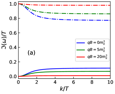
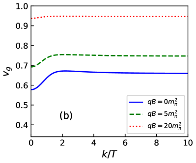
Figure 1: (Color online) The imaginary parts of the dispersion relations obtain from eq. (60) for $\theta=\frac{\pi}{2}$ with different magnetic fields denoted by different colors. The blue, green and red colors correspond to $B_{0}=$ 0, $5m_{\pi}^{2}$ and $20m_{\pi}^{2}$, respectively. In left panel the solid lines are for the propagating modes $(\omega_{2,3})$ and the dashed lines are for the non-propagating mode $(\omega_{1})$. The other parameters used are $a_{1}=0.1$, $\alpha=1/3$, $T=200\,$MeV, $\tau_{\Pi}$=0.985 fm and kept fixed for all the curves.

If we take the small $k$ limit, Eqs. (59) and (60) yield the following modes:

$$\omega=\left\{\begin{array}[]{l}{\frac{i}{\tau_{\Pi}}},\\ \pm kv_{A}\cos{\theta},\\ {\pm kv_{M}}.\end{array}\right.$$ (69)

For this case the group velocity is observed to be same as the velocity for the ideal MHD.

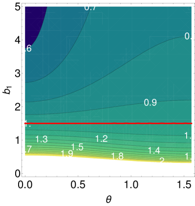
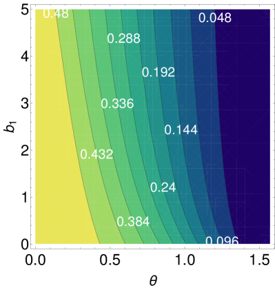
Figure 2: (Color online) Contour plot showing various causal regions, obtained from eq. (72), for fast (left panel) and slow (right panel) branches. The red contour is the critical line of causality, denoting $v_{L}^{2}=1$. The region above the red line is causal for the fast magneto-sonic waves and acausal below. The slow branch is causal throughout the parameter space. The magnitude of the magnetic field has been fixed to $qB=10m^{2}_{\pi}$ and the other parameters used are $\alpha=1/3$, $T=200\,$MeV.

We analyse the causality of the system by following ref. Pu:2009fj where it was shown that to guarantee the causality requires that the asymptotic value of the group velocity should be less than the speed of light. Alfvén mode in eq. (59) remains unaffected due to the bulk viscosity and hence always remain causal. For the magneto-sonic waves in the large $k$ limit, we take the following ansatz $\omega=v_{L}k$ in eq. (60) and collect terms in the leading-order of $k$, this yields

$$v_{L}^{4}-xv_{L}^{2}+y=0,$$ (70)

where

$$x=v_{A}^{2}+\left(\alpha+\frac{1}{b_{1}}\right)\left(1-v_{A}^{2}\sin^{2}{\theta}\right),$$

$$y=\left(\alpha+\frac{1}{b_{1}}\right)v_{A}^{2}\cos^{2}{\theta}.$$ (71)

The velocities $v_{L}$ are

$$v_{L}^{2}=\frac{1}{2}\left(x\pm\sqrt{x^{2}-4y}\right).$$ (72)

Here, we see that unlike the small $k$ limit, at large $k$ the group velocity is affected by the transport coefficients. In order to have causal propagation, one demands $v_{L}^{2}\leq 1$, which yields a causal parameter-set for the two branches, which correspond to the fast or slow magneto-sonic modes

fast: $$(0<y<1)\land(2\sqrt{y}\leq x<y+1),$$

slow: $$\left[\left(0<y<1\right)\land\left(x\geq 2\sqrt{y}\right)\right]\lor\left[(y\geq 1)\land(x>y+1)\right]$$ (73)

Contour plot of the various causal regions is shown in Fig. 2, where $b_{1}$ is defined in eq. (15). For the fast branch, we find that, although the asymptotic velocities depend on the magnitude of the magnetic field and the direction $\theta$, the critical value, i.e., $b_{1}=1.5$ (red solid line), is independent of them. The slow branch is similarly $B$ and $\theta$ dependent but moreover is causal throughout the parameter space.

4.3 MHD with shear viscosity

Many theoretical studies indicate that shear viscosity over entropy $\eta/s$ has a minimum near the crossover temperature $T_{co}$ and rises as a function of temperature on both sides of $T_{co}$ in ref. Kovtun:2004de . Although such studies indicate $\eta/s$ to be temperature dependent, nevertheless that would require an additional parametrization of $\eta/s$ which should come from the underlying theory. For simplicity, we will assume in the foregoing section $\eta/s$ is a constant.

The energy-momentum tensor for a fluid with zero bulk and non-zero shear viscosity in a magnetic field takes the following form

$$T^{\mu\nu}=\left(\varepsilon+P+B^{2}\right)u^{\mu}u^{\nu}-\left(P+\frac{B^{2}}{2}\right)g^{\mu\nu}-B^{2}b^{\mu}b^{\nu}+\pi^{\mu\nu}.$$ (74)

According to the IS second-order theories of relativistic dissipative fluid dynamics, the space-time evolutions of the shear stress tensor are given by eq. (11). For a given perturbation in the fluid, the energy-momentum tensor and the shear stress tensor can be decomposed as

$$T^{\mu\nu} = T_{0}^{\mu\nu}+\delta\tilde{T}^{\mu\nu},$$ (75)

$$\pi^{\mu\nu} = \pi_{0}^{\mu\nu}+\delta\tilde{\pi}^{\mu\nu}.$$ (76)

Where the perturbed energy-momentum tensor is

$$\delta{\tilde{T}}^{\mu\nu} =\left(\varepsilon_{0}+P_{0}+B_{0}^{2}\right)\left(u_{0}^{\mu}\delta{\tilde{u}}^{\nu}+\delta{\tilde{u}}^{\mu}u_{0}^{\nu}\right)+\left(\delta{\tilde{\varepsilon}}+\delta{\tilde{P}}+2B_{0}\delta{\tilde{B}}\right)u_{0}^{\mu}u_{0}^{\nu}$$ (77)

$$-\left(\delta{\tilde{P}}+B_{0}\delta{\tilde{B}}\right)g^{\mu\nu}-B_{0}^{2}\left(b_{0}^{\mu}\delta{\tilde{b}}^{\nu}+\delta{\tilde{b}}^{\mu}b_{0}^{\nu}\right)-2B_{0}\delta{\tilde{B}}b_{0}^{\mu}b_{0}^{\nu}+\delta\tilde{\pi}^{\mu\nu}.$$

As usual, to solve the set of equations eq. (11), the conservation of the perturbed energy-momentum tensor [eq. (77)], and eqs. (36)-(39) for obtaining the dispersion relation we write them in a matrix form

$$A\delta\tilde{X}^{T}=0,$$ (78)

where $\delta\tilde{X}=(\delta\tilde{\varepsilon},\delta\tilde{u}^{x},\delta\tilde{u}^{y},\delta\tilde{u}^{z},\delta\tilde{b}^{x},\delta\tilde{b}^{y},\delta\tilde{\pi}^{xx},\delta\tilde{\pi}^{xy},\delta\tilde{\pi}^{xz},\delta\tilde{\pi}^{yy},\delta\tilde{\pi}^{yz})$ and the matrix $A$ given in eq. (154). The $\det(A)=0$ gives

$$\left(1+i\omega\tau_{\pi}\right)^{2} = 0,$$ (79)

$$\omega^{3}-\frac{i}{\tau_{\pi}}\omega^{2}-\left(v_{A}^{2}\cos^{2}{\theta}+\frac{\eta}{h\tau_{\pi}}\right)k^{2}\omega+\frac{i}{\tau_{\pi}}k^{2}v_{A}^{2}\cos^{2}{\theta} = 0,$$ (80)

$$\omega^{6}+\mathsf{X}_{5}\omega^{5}+\mathsf{X}_{4}\omega^{4}+\mathsf{X}_{3}\omega^{3}+\mathsf{X}_{2}\omega^{2}+\mathsf{X}_{1}\omega+\mathsf{X}_{0} = 0,$$ (81)

where

$$\mathsf{X}_{5} = -\frac{2i}{\tau_{\pi}},$$

$$\mathsf{X}_{4} = -\frac{1}{\tau_{\pi}^{2}}-\left[\mathsf{Y}+\frac{1}{3b}\left\{7-v_{A}^{2}\left(3+\sin^{2}{\theta}\right)\right\}\right]k^{2},$$

$$\mathsf{X}_{3} = \frac{i}{\tau_{\pi}}\left[2\mathsf{Y}+\frac{1}{3b}\left\{7-v_{A}^{2}\left(3+\sin^{2}{\theta}\right)\right\}\right]k^{2},$$

$$\mathsf{X}_{2} = \frac{\mathsf{Y}}{\tau_{\pi}^{2}}k^{2}+\left[\alpha\left(v_{A}^{2}\cos^{2}{\theta}+\frac{\eta}{h\tau_{\pi}}\right)+\frac{1}{3b}\left\{\frac{4\eta}{h\tau_{\pi}}+v_{A}^{2}\left(3+\sin^{2}{\theta}\right)\right\}\right]k^{4},$$

$$\mathsf{X}_{1} = -\frac{i}{\tau_{\pi}}\left[\alpha\left(2v_{A}^{2}\cos^{2}{\theta}+\frac{\eta}{h\tau_{\pi}}\right)+\frac{v_{A}^{2}}{3b}\left(3+\cos^{2}{\theta}\right)\right]k^{4},$$

$$\mathsf{X}_{0} = -\frac{\alpha}{\tau_{\pi}^{2}}v_{A}^{2}k^{4}\cos^{2}{\theta},\hskip 28.45274pt\hskip 28.45274pt\mathsf{Y}=v_{A}^{2}+\alpha\left(1-v_{A}^{2}\sin^{2}{\theta}\right).$$ (82)

Note that the term $b$ of eq. (23) in the above equations can be recast into $b\equiv\frac{h\tau_{\pi}}{\eta}(1-v_{A}^{2})$. From eq. (79) we get two non-propagating and stable modes as

$$\omega=\frac{i}{\tau_{\pi}}.$$ (83)

Equation (80) is a third-order polynomial equation and the analytic solution for this type of equation is discussed in appendix A. Equation (81) is a sixth-order polynomial equation which is impossible to solve analytically. We can still gain some insight for a few special cases which are discussed below.

For $\theta=0$, eq. (80) still remains a third-order polynomial equation and the coefficients of that polynomial can easily be obtained from eq. (80) as

$$X_{0} =\frac{i}{\tau_{\pi}}v_{A}^{2}k^{2}, X_{1} =-\left(v_{A}^{2}+\frac{\eta}{h\tau_{\pi}}\right)k^{2}, X_{2} =-\frac{i}{\tau_{\pi}}.$$ (84)

On the other hand, eq. (81) can be factorized into two third-order polynomial equations. The coefficients of one of such the third-order polynomial equation are

$$X_{0} =\frac{i\alpha}{\tau_{\pi}}k^{2}, X_{1} =-\left(\alpha+\frac{4}{3b}\right)k^{2}, X_{2} =-\frac{i}{\tau_{\pi}},$$ (85)

whereas the coefficients of the remaining other third-order polynomial equation from eq. (81) are same as eq. (84)

The roots of these third order polynomial equations are discussed in appendix A with the given $X_{i}$s. We checked that the dispersion relations obtained from these equations with the coefficients given in eq. (85) are same as the sound mode in ref. Pu:2009fj .

For $\theta=\pi/2$, one root of eq. (80) vanish and other two roots are of the form

$$\omega=\frac{1}{2\tau_{\pi}}\left(i\pm\sqrt{\frac{4\eta\tau_{\pi}}{h}k^{2}-1}\right).$$ (86)

From eq. (81), one of the root vanish and other two roots are of the form

$$\omega=\frac{1}{2\tau_{\pi}}\left(i\pm\sqrt{\frac{4\eta\tau_{\pi}}{\varepsilon_{0}+P_{0}}k^{2}-1}\right).$$ (87)

The remaining three modes from eq. (81), are obtained from a cubic polynomial with $X_{i}$’s given as:

$$X_{0} =\frac{i}{\tau_{\pi}}v_{f}^{2}k^{2}, X_{1} =-\left(v_{f}^{2}+\frac{4\eta}{3h\tau_{\pi}}\right)k^{2}, X_{2} =-\frac{i}{\tau_{\pi}}.$$ (88)

The corresponding roots can be calculated using the formula given in appendix A.

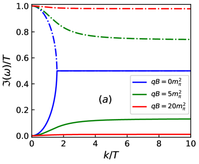
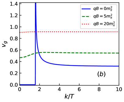
Figure 3: (Color online) The left panel shows the imaginary parts of the dispersion relations and the right panel shows the group velocities obtained from a cubic polynomial with the coefficients given in eq. (84) for $\theta=0$. The other parameters used are $a=0.1,\alpha=1/3,T=200\,\text{MeV},\tau_{\pi}=0.985\,\text{fm}$ and their values are kept fixed for all the curves. In the left panel, the solid lines are for $\Im(\omega_{2,3})$ which are degenerate. The dash-dotted lines correspond to $\Im{(\omega_{1})}$.

The left panel of Fig. 3 shows the dependence of the imaginary parts of $\omega$ as a function of $k/T$ and the right panel shows the group velocity as a function of $k/T$ for different values of magnetic field for $\theta=0$. Various lines corresponds to different magnetic fields: $qB=0$ (blue lines), $qB=5m_{\pi}^{2}$ (green lines), $qB=20m_{\pi}^{2}$ (red lines). Fig. 4 shows the same thing but for $\theta=\frac{\pi}{2}$ (eq. (88)).

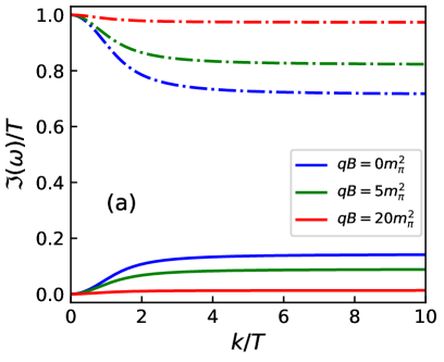
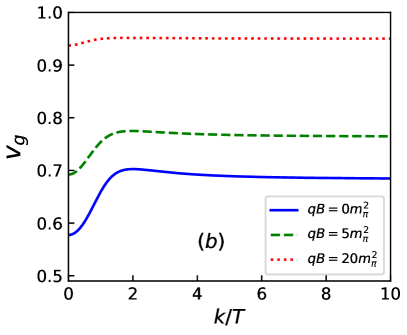
Figure 4: (Color online) The left panel shows the imaginary parts of $\omega$ and the right panel shows the group velocities obtained from the cubic polynomial with the coefficient given in eq. (88) for $\theta=\frac{\pi}{2}$. The other parameters used are $a=0.1,\alpha=1/3,T=200\,\text{MeV},\tau_{\pi}=0.985\,\text{fm}$ and are kept fixed for all the curves.In the left panel, the dash-dotted lines represent $\Im{(\omega_{1})}$ and the solid lines are for $\Im(\omega_{2,3})$ which are also degenerate.

In the small $k$ limit the dispersion relations that we get from eqs. (79)-(81) are

$$\omega=\left\{\ \begin{array}[]{ll}\frac{i}{\tau_{\pi}},\\ \pm kv_{A}\cos{\theta},\\ \pm kv_{M}.\end{array}\right.$$ (92)

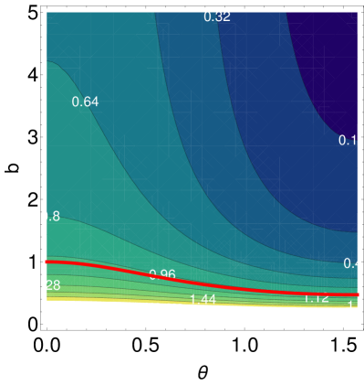
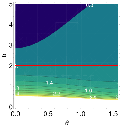
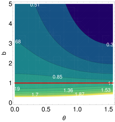
Figure 5: (Color online) Contour plot showing various causal regions, obtained from eq. (95), for Alfvén mode (top left) and the set of fast (top right) and slow modes (bottom) from eq. (95). The red contour is the critical line of causality, denoting $v_{L}^{2}=1$. The region above the red line is causal and below it corresponds to the acausal zone. The magnitude of the magnetic field has been fixed to $qB=10m^{2}_{\pi}$ and the other parameters used are $\alpha=1/3$, $T=200\,$MeV.

Note that the first root have a degeneracy five.

In the large $k$ limit we use the ansatz $\omega=v_{L}k$ and keep only the leading-order terms in $k$, then the velocities $v_{L}$ are

$$v_{L}^{2}=\left\{\ \begin{array}[]{ll}v_{A}^{2}\cos^{2}{\theta}+\frac{\eta}{h\tau_{\pi}},\\ \frac{1}{2}\left[x\pm\sqrt{x^{2}-4y}\right],\end{array}\right.$$ (95)

where

$$x=v_{A}^{2}+\alpha\left(1-v_{A}^{2}\sin^{2}{\theta}\right)+\frac{1}{3b}\left\{\ 7-v_{A}^{2}\left(3+\sin^{2}{\theta}\right)\right\}\ ,$$

$$y=\alpha\left(v_{A}^{2}\cos^{2}{\theta}+\frac{\eta}{h\tau_{\pi}}\right)+\frac{1}{3b}\left\{\ v_{A}^{2}\left(3+\cos^{2}{\theta}\right)+\frac{4\eta}{h\tau_{\pi}}\right\}\ .$$ (96)

The asymptotic causality condition for the shear-Alfvén mode can readily be obtained as

shear-Alfvén: $$v_{A}^{2}\cos^{2}{\theta}+\frac{(\varepsilon+P)}{hb}\leq 1,$$ (97)

where $b$ is defined in eq. (23). We observe that in this case the wave velocity and the causality conditions depend on both the magnitude of the magnetic field and direction of propagation of the perturbation. To explore the inter-dependency we show various causal regions as a function of $b$ and $\theta$ as a contour plot in Fig. 5 (top left). We notice that the critical value of $b$ at $\theta=0$ is $b_{c}=1$ and this value is independent of magnitude of the magnetic field. In the other extreme, i.e. for $\theta=\pi/2$, the critical value is $b_{c}=[1+B^{2}/(\varepsilon+P)]^{-1}$ , i.e., $b_{c}$ decreases with increasing magnetic field. In the limit of vanishing magnetic field it has been found in ref. Pu:2009fj that for causal propagation of the shear modes $b\geq 1$ should be satisfied. In the presence of magnetic field we found that, this constraint can be relaxed to even smaller values of $b$, given that the waves move obliquely.

The causality constraint of the fast and slow waves in eq. (95) can be written in the form of (4.2). The simplified expression for the magneto-sonic modes can be written as

fast: $$(0<y<1)\land(2\sqrt{y}\leq x<y+1),$$

slow: $$\left[\left(0<y<1\right)\land\left(x\geq 2\sqrt{y}\right)\right]\lor\left[(y\geq 1)\land(x>y+1)\right].$$ (98)

We show various causal regions as a function of $b$ and $\theta$ as a contour plot in Fig. 5 (top right and bottom). The critical value of $b$, i.e., $b_{c}=2$ (obtained from (95)) is independent of the angle $\theta$ and the magnitude of magnetic field for the fast magneto-sonic mode. In the absence of a magnetic field this value coincides with that obtained for the sound mode in ref. Pu:2009fj . Similarly, the slow magneto-sonic mode yields the critical value of $b_{c}=1$, independent of the angle $\theta$ and the magnitude of magnetic field $B$. It is still interesting to see that although the critical values of the fast and slow modes are $B$ and $\theta$ independent, the asymptotic velocities are nevertheless dependent. Increasing the magnetic field, increases the asymptotic group velocities but the causal region always remains causal no matter how large the magnetic field becomes.

4.4 MHD with both bulk and shear viscosity

In this subsection, we investigate the stability and causality of a viscous fluid with finite shear and the bulk viscosity in a magnetic field.

In heavy-ion collisions the initial magnetic field is very large and both shear and bulk viscosities are non-zero for the temperature range achieved in these collisions, hence the present case is most relevant to the actual heavy-ion collisions at top RHIC and LHC energies. The energy-momentum tensor is

$$T^{\mu\nu}=\left(\varepsilon+P+\Pi+B^{2}\right)u^{\mu}u^{\nu}-\left(P+\Pi+\frac{B^{2}}{2}\right)g^{\mu\nu}-B^{2}b^{\mu}b^{\nu}+\pi^{\mu\nu}.$$ (99)

The small variation of the energy-momentum tensor due to the perturbed fields is

$$\delta{\tilde{T}}^{\mu\nu} =\left(\varepsilon_{0}+P_{0}+B_{0}^{2}\right)\left(u_{0}^{\mu}\delta{\tilde{u}}^{\nu}+\delta{\tilde{u}}^{\mu}u_{0}^{\nu}\right)+\left(\delta{\tilde{\varepsilon}}+\delta{\tilde{P}}+\delta{\tilde{\Pi}}+2B_{0}\delta{\tilde{B}}\right)u_{0}^{\mu}u_{0}^{\nu}$$ (100)

$$-\left(\delta{\tilde{P}}+\delta{\tilde{\Pi}}+B_{0}\delta{\tilde{B}}\right)g^{\mu\nu}-B_{0}^{2}\left(b_{0}^{\mu}\delta{\tilde{b}}^{\nu}+\delta{\tilde{b}}^{\mu}b_{0}^{\nu}\right)-2B_{0}\delta{\tilde{B}}b_{0}^{\mu}b_{0}^{\nu}+\delta\tilde{\pi}^{\mu\nu}.$$

Following the same procedure, as discussed in the previous two sections, we obtain the dispersion relations for the following independent variables

$$\delta\tilde{X}=(\delta\tilde{\varepsilon},\delta\tilde{u}^{x},\delta\tilde{u}^{y},\delta\tilde{u}^{z},\delta\tilde{b}^{x},\delta\tilde{b}^{y},\delta\tilde{\pi}^{xx},\delta\tilde{\pi}^{xy},\delta\tilde{\pi}^{xz},\delta\tilde{\pi}^{yy},\delta\tilde{\pi}^{yz},\delta\tilde{\Pi})^{T}.$$ (101)

Following the usual procedure of linearisation we get a $12\times 12$ dimensional square matrix $A$. By setting $\det{A}=0$ we have the following equations which subsequently give the dispersion relations

$$\left(1+i\omega\tau_{\pi}\right)^{2}=0,$$ (102)

$$\omega^{3}-\frac{i}{\tau_{\pi}}\omega^{2}-\left(v_{A}^{2}\cos^{2}{\theta}+\frac{\eta}{h\tau_{\pi}}\right)k^{2}\omega+\frac{i}{\tau_{\pi}}k^{2}v_{A}^{2}\cos^{2}{\theta}=0,$$ (103)

$$\omega^{7}+\mathsf{X}_{6}\omega^{6}+\mathsf{X}_{5}\omega^{5}+\mathsf{X}_{4}\omega^{4}+\mathsf{X}_{3}\omega^{3}+\mathsf{X}_{2}\omega^{2}+\mathsf{X}_{1}\omega+\mathsf{X}_{0}=0,$$ (104)

where

$$\mathsf{X_{6}} = -i\left(\frac{1}{\tau_{\Pi}}+\frac{2}{\tau_{\pi}}\right),$$

$$\mathsf{X}_{5} = -\frac{1}{\tau_{\pi}}\left(\frac{2}{\tau_{\Pi}}+\frac{1}{\tau_{\pi}}\right)-\left[v_{A}^{2}+\left(\alpha+\frac{1}{b_{1}}\right)\left(1-v_{A}^{2}\sin^{2}{\theta}\right)+\frac{1}{3b}\left\{\ 7-v_{A}^{2}\left(3+\sin^{2}{\theta}\right)\right\}\right]k^{2},$$

$$\mathsf{X}_{4} = \frac{i}{\tau_{\pi}^{2}\tau_{\Pi}}+i\biggl{[}\left(\frac{1}{\tau_{\Pi}}+\frac{2}{\tau_{\pi}}\right)Y+\frac{2}{b_{1}\tau_{\pi}}\left(1-v_{A}^{2}\sin^{2}{\theta}\right)+\frac{1}{3b}\left(\frac{1}{\tau_{\pi}}+\frac{1}{\tau_{\Pi}}\right)\Big{\{}7-v_{A}^{2}\left(3+\sin^{2}{\theta}\right)\Big{\}}\biggr{]}k^{2},$$

$$\mathsf{X}_{3} = \biggl{[}\frac{1}{b_{1}\tau_{\pi}^{2}}\left(1-v_{A}^{2}\sin^{2}{\theta}\right)+\frac{1}{3b\tau_{\pi}\tau_{\Pi}}\left\{\ 7-v_{A}^{2}\left(3+\sin^{2}{\theta}\right)\right\}\ +\left(\frac{2}{\tau_{\Pi}\tau_{\pi}}+\frac{1}{\tau_{\pi}^{2}}\right)Y\biggr{]}k^{2}$$

$$+\left[\left(\alpha+\frac{1}{b_{1}}\right)\left(v_{A}^{2}\cos^{2}{\theta}+\frac{\eta}{h\tau_{\pi}}\right)+\frac{1}{3b}\left\{(v_{A}^{2}\left(3+\cos^{2}{\theta}\right)+\frac{\eta}{3h\tau_{\pi}}\right\}\right]k^{4},$$

$$\mathsf{X}_{2} = -\frac{i}{\tau_{\pi}^{2}\tau_{\Pi}}\mathsf{Y}k^{2}-i\Biggl{[}\frac{1}{b_{1}\tau_{\pi}}\left(2v_{A}^{2}\cos^{2}{\theta}+\frac{\eta}{h\tau_{\pi}}\right)+\frac{1}{3b\tau_{\Pi}}\left\{v_{A}^{2}\left(\frac{1}{\tau_{\Pi}}+\frac{1}{\tau_{\pi}}\right)\left(3+\cos^{2}{\theta}\right)+\frac{4\eta}{3h\tau_{\pi}}\right\}$$

$$+\alpha\left\{\ \frac{\left(1-v_{A}^{2}\right)}{b}\left(\frac{1}{\tau_{\Pi}}+\frac{1}{\tau_{\pi}}\right)+v_{A}^{2}\left(\frac{1}{\tau_{\Pi}}+\frac{2}{\tau_{\pi}}\right)\right\}\Biggr{]}k^{4},$$

$$\mathsf{X}_{1} = -\left[\frac{v_{A}^{2}}{b_{1}\tau_{\pi}^{2}}\cos^{2}{\theta}+\frac{v_{A}^{2}}{3b\tau_{\pi}\tau_{\Pi}}\left(3+\cos^{2}{\theta}\right)+\frac{\alpha\eta}{h\tau_{\pi}\tau_{\Pi}}+\alpha v_{A}^{2}\left(\frac{2}{\tau_{\pi}\tau_{\Pi}}+\frac{1}{\tau_{\pi}^{2}}\right)\cos^{2}{\theta}\right]k^{2},$$

$$\mathsf{X}_{0} = \frac{\alpha v_{A}^{2}}{\tau_{\pi}^{2}\tau_{\Pi}}k^{4}\cos^{2}{\theta},\hskip 42.67912pt\mathsf{Y}=v_{A}^{2}+\alpha\left(1-v_{A}^{2}\sin^{2}{\theta}\right).$$ (105)

First, we find that eq. (102) gives two non-propagating modes of frequency $\omega=\frac{i}{\tau_{\pi}}$. Now, the eq. (103) is a third-order polynomial and can be solved analytically as discussed previously whereas the eq. (104) is a seventh-order polynomial equation and can not be solved analytically, therefore we lookout for the solution of these equations for some special cases discussed below.

For $\theta=0$, we obtain two cubic and a single quartic equations. The $X_{i}$’s of the two cubic polynomials are same as in eq. (84). The dispersion relations for these cases are already discussed in the previous section, hence we will not repeat them here. The $X_{i}$’s for the fourth-order polynomial equation are

$$X_{3} =-i\left(\frac{1}{\tau_{\pi}}+\frac{1}{\tau_{\Pi}}\right), X_{2} =-\frac{1}{\tau_{\pi}\tau_{\Pi}}-\left(\alpha+\frac{1}{b_{1}}+\frac{4}{3b}\right)k^{2},$$

$$X_{1} =i\left[\alpha\left(\frac{1}{\tau_{\pi}}+\frac{1}{\tau_{\Pi}}\right)+\frac{1}{b_{1}\tau_{\pi}}+\frac{4}{3b\tau_{\Pi}}\right]k^{2}, X_{0} =\frac{\alpha}{\tau_{\pi}\tau_{\Pi}}k^{2},$$ (106)

and the corresponding roots can be calculated using the formula given in Appendix A.

For another case, we choose $\theta=\frac{\pi}{2}$, this time two of the roots turned out to be zero, and another two roots are the same as eq. (87). As before, we call these four modes as shear mode. The $X_{i}$’s for the fourth-order polynomial equation are

$$X_{0}=\frac{1}{\tau_{\pi}\tau_{\Pi}}v_{f}^{2}k^{2},$$

$$X_{1}=i\left[\left(\frac{1}{\tau_{\pi}}+\frac{1}{\tau_{\Pi}}\right)v_{f}^{2}+\frac{1}{h\tau_{\pi}\tau_{\Pi}}\left(\zeta+\frac{4}{3}\eta\right)\right]k^{2},$$

$$X_{2}=-\frac{1}{\tau_{\pi}\tau_{\Pi}}-\left[v_{f}^{2}+\frac{1}{h}\left(\frac{\zeta}{\tau_{\Pi}}+\frac{4\eta}{3\tau_{\pi}}\right)\right]k^{2},$$

$$X_{3}=-i\left(\frac{1}{\tau_{\pi}}+\frac{1}{\tau_{\Pi}}\right),$$ (107)

and the corresponding roots can be calculated using the formula given in Appendix A.

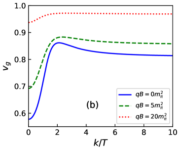
Figure 6: (Color online) In the left panel $\Im(\omega)/T$ versus $k/T$ and in the right panel group velocity as a function of $k/T$ are plotted for different magnetic fields for $\theta=\frac{\pi}{2}$. $v_{g}$ is obtained from a quartic equation with the coefficients eq. (4.4). The solid lines in the left panel corresponds to the propagating modes, the dashed lines and the dash-dotted lines correspond the non-propagating modes. The other parameters used here are $a=a_{1}=0.1,T=200\,\text{MeV},\tau_{\Pi}=0.985\,\text{fm}\ \text{and}\ \tau_{\pi}=0.591\,\text{fm}$ and kept constants for all the curves.

Note that the imaginary part of the propagating modes (obtained from eq. (4.4)) are degenerate and hence not shown separately in Fig. 6. The dash-dotted lines in the left panel of Fig. 6 correspond to the non-propagating modes generated due to the bulk viscosity, this is because in the small $k$ limit they reduce to $\frac{i}{\tau_{\Pi}}$, and in the same logic the dotted line corresponds to the non-propagating mode due to the shear viscosity. In general, we find that the $\Im(\omega)$ is always positive for our set-up. So, for this parameter set, the fluid is always stable under small perturbation for non-zero bulk and shear viscosity. Also, we note another interesting point, when the magnetic field is increased the imaginary part of the propagating mode tends to zero i.e, the damping of the perturbation diminishes.

In the small $k$ limit the dispersion relations from eqs. (102)-(104) become

$$\omega=\left\{\begin{array}[]{ll}\frac{i}{\tau_{\pi}},\\ \frac{i}{\tau_{\Pi}},\\ \pm kv_{A}\cos{\theta},\\ \pm kv_{M},\end{array}\right.$$ (112)

here also the first root have degeneracy of five. Similarly, in the large $k$ limit using the ansatz $\omega=v_{L}k$, we obtain the asymptotic group velocities $v_{L}$ as:

$$v_{L}^{2}=\left\{\ \begin{array}[]{ll}v_{A}^{2}\cos^{2}{\theta}+\frac{\eta}{h\tau_{\pi}},\\ \frac{1}{2}\left[x\pm\sqrt{x^{2}-4y}\right],\end{array}\right.$$ (115)

where

$$x=\left[v_{A}^{2}+\left(\alpha+\frac{1}{b_{1}}\right)\left(1-v_{A}^{2}\sin^{2}{\theta}\right)+\frac{1}{3b}\left\{\ 7-v_{A}^{2}\left(3+\sin^{2}{\theta}\right)\right\}\ \right],$$

$$y=\left[\left(\alpha+\frac{1}{b_{1}}\right)v_{A}^{2}\cos^{2}{\theta}+\left(\alpha+\frac{1}{b_{1}}+\frac{4}{3b}\right)\frac{\eta}{h\tau_{\pi}}+\frac{v_{A}^{2}}{3b}\left(3+\cos^{2}{\theta}\right)\right].$$ (116)

Now we are ready to explore the causality of a fluid in magnetic field. For this, we again check whether the asymptotic group velocity has super or sub luminal speed. We found that the theory as a whole is causal if the fluid satisfy the following asymptotic causality conditions for magneto-sonic waves:

fast: $$(0<y<1)\land(2\sqrt{y}\leq x<y+1),$$

slow: $$\left[\left(0<y<1\right)\land\left(x\geq 2\sqrt{y}\right)\right]\lor\left[(y\geq 1)\land(x>y+1)\right].$$ (117)

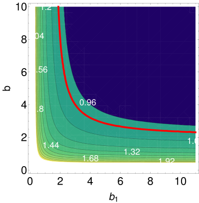
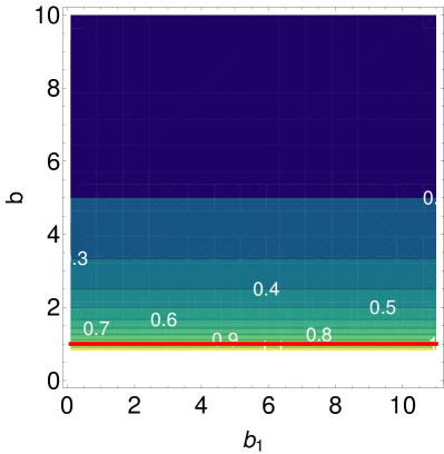
Figure 7: (Color online) Contour plot showing various causal regions, obtained from eq. (4.4), for fast (left panel) and slow (right panel) branches. The red contour is the critical line of causality, denoting $v_{L}^{2}=1$. The region above the red line is causal for the slow magneto-sonic waves and acausal below similarly for the fast magneto-sonic wave right side of red line is causal region and left side is acausal region. The magnitude of the magnetic field has been fixed to $qB=10m^{2}_{\pi}$ and the other parameters used are $\alpha=1/3$, $T=200\,$MeV.

From eq. (115) we find that a larger magnetic field gives a larger $v_{L}$, but always remain sub-luminal given $b$ and $b_{1}$ are larger than their corresponding critical values (discussed earlier). It is also clear from eq. (115) the asymptotic group velocity for non-zero bulk and shear viscosity is larger than the individual shear and bulk viscous cases.

In Fig. 7 we show the contour plot of various causal regions as a function of $b$ and $\theta$. The critical line (red line) of the fast magneto-sonic mode (left panel) show that $b$ and $b_{1}$ are inversely proportional. On the other hand, the causality condition for the slow magneto-sonic waves is independent of $b_{1}$. The critical value of $b$ for the slow magneto-sonic mode is $b_{c}=1$.

5 Characteristic velocities for bulk viscosity

The characteristic curves can be seen as the lines along which any information is transported in the fluid, for example small perturbations, discontinuities, defects or shocks etc travel along one of these characteristic curves refs. Sommerfeld ; Hilbert ; rezzolla2013relativistic . Here we take the effect of non-linearity in the propagation speed which is ignored in the linearisation procedure discussed earlier. Without the loss of generality we consider the ($2+1$)-dimensional case with only bulk viscosity (shear viscosity can be added in the similar way) and write the energy-momentum conservation equations, Maxwell’s equations and the IS equation in the standard form for studying the characteristic velocities as

$$P^{\beta}_{mn}\partial_{\beta}Q^{n}+R_{m}=0.$$ (118)

Here $Q^{n}=\left(\varepsilon,u^{x},u^{y},b^{x},B,\Pi\right)$ and $R_{m}=\left(0,0,0,0,0,\Pi\right)$. We parametrize the fluid velocity as $u^{\mu}=\left(\cosh{\theta},\sinh{\theta}\cos{\phi},\sinh{\theta}\sin{\phi},0\right)$ and the $b^{\mu}=\left(\sinh{\theta},\cosh{\theta}\cos{\phi},\cosh{\theta}\sin{\phi},0\right)$. The matrix elements of $P^{t}_{mn},P^{x}_{mn},P^{y}_{mn}$ are given in Appendix B.

We find the characteristic velocities ($v_{x}^{ch},v_{y}^{ch}$) by solving the following equations:

$$\det\left(v_{x}^{ch}P^{t}-P^{x}\right)=0,$$ (119)

$$\det\left(v_{y}^{ch}P^{t}-P^{y}\right)=0.$$ (120)

For simplicity, here we take fluid in the LRF i.e, $u^{\mu}=\left(1,0,0,0\right)$ and the magnetic filed along the $y$-axis $b^{\mu}=\left(0,0,1,0\right)$. Then the characteristic velocities are

$$v_{x}^{ch}=\pm\sqrt{\frac{B^{2}+\alpha\left(\varepsilon+P+\Pi\right)}{\left(h+\Pi\right)}+\frac{\zeta}{\tau_{\Pi}\left(h+\Pi\right)}},$$ (121)

$$v_{y}^{ch}=\left\{\begin{array}[]{ll}\pm\frac{B}{\sqrt{\left(h+\Pi\right)}},\\ \\ \pm\sqrt{\alpha+\frac{\zeta}{\tau_{\Pi}\left(\varepsilon+P+\Pi\right)}},\end{array}\right.$$ (122)

where $h=\varepsilon+P+B^{2}$ and the other roots are zero. The characteristic velocities obtain in eqs. (121), (122) are same with the eq. (72) for $\theta=\frac{\pi}{2}$ and $\theta=0$, respectively provide $\Pi=0$. So we conclude that the asymptotic group velocity obtained by linearizing the MHD-IS equations is same as the characteristic velocities.

6 Results from the modified IS theory

In fact, the formulation of second order hydrodynamical theory in the presence of electromagnetic field is still an active area of research. So far all the results we discussed were obtained for viscous fluid in a magnetic field within the frame-work of the IS theory. The IS relaxation eq. (11) do not consider the effect of magnetic field. However, recently the authors of ref. Denicol:2018rbw solved the Boltzmann equation in the presence of magnetic field using the 14 moment approximation and found that IS relaxation eq. (11) gets modified. We call these equations the modified IS equations or the NRMHD-IS (non-resistive MHD-IS) equations. The NRMHD-IS equations shows that the relaxation equation for the shear-stress tensor contains additional terms, here we neglected most of the terms and only keep the term which couples magnetic field and the shear viscosity. The simplified NRMHD-IS equation takes the following form

$$\tau_{\pi}\frac{d}{d\tau}\pi^{<\mu\nu>}+\pi^{\mu\nu}=2\eta\sigma^{\mu\nu}-\delta_{\pi B}Bb^{\alpha\beta}\Delta^{\mu\nu}_{\alpha\kappa}g_{\lambda\beta}\pi^{\kappa\lambda}.$$ (123)

Where $\delta_{\pi B}$ is a new coefficient appearing only due to the magnetic field and $b^{\alpha\beta}=-\epsilon^{\alpha\beta\gamma\delta}u_{\gamma}b_{\delta}$ is an anti-symmetric tensor which satisfy $b^{\mu\nu}u_{\nu}=b^{\mu\nu}b_{\nu}=0$. The rank-four traceless and symmetric projection operator is defined as $\Delta^{\mu\nu}_{\alpha\kappa}=\frac{1}{2}\left(\Delta^{\mu}_{\alpha}\Delta^{\nu}_{\kappa}+\Delta^{\mu}_{\kappa}\Delta^{\nu}_{\alpha}\right)-\frac{1}{3}\Delta^{\mu\nu}\Delta_{\alpha\kappa}$.

Before proceeding further, a few comments on the NRMHD-IS equations are in order. It is well known that in the presence of a magnetic field, the transport coefficients split into several components, namely three bulk components and five shear components refs. Grozdanov:2016tdf ; Hernandez:2017mch ; Denicol:2018rbw ; Dash:2020vxk . The information of these anisotropic transport coefficients are hidden inside the new coupling terms of the modified IS theory eq. (123). Note that the first-order terms on the right-hand sides are proportional to the usual shear-viscosity. These terms can be combined with the first-order terms on the left-hand side and, after inversion of the respective coefficient matrices, will lead to the various anisotropic transport coefficients. On the other hand, when solving the full second-order equations of the modified IS theory, one does not need to replace the standard viscosity with the anisotropic transport coefficients, since the effect of the magnetic field, is already taken into account by the new terms in these equations. Regarding modified second-order theory with finite bulk viscosity, we would like to mention that, there is still no existing theory that yields three distinct bulk components in Navier-Stokes limit (for details see ref. Denicol:2018rbw ) and it is still an open issue.

The last term of eq. (123) is the only non-trivial term added to the conventional IS theory for which we already discussed the results in previous sections. So, here we only consider the last term of eq. (123) and calculate the corresponding correction to the old results.

First, we add a perturbation to the new term which contributes to $\delta\tilde{\pi}^{\mu\nu}$

$$\delta{\tilde{I}}^{\mu\nu} = \delta_{\pi B}B_{0}b^{\alpha\beta}_{0}\Delta^{\mu\nu}_{\alpha\kappa}g_{\lambda\beta}\delta{\tilde{\pi}^{\kappa\lambda}}.$$ (124)

While calculating eq. (124) we use the fact that in the local rest frame the unperturbed shear stress tensor vanishes i.e., $\pi^{\mu\nu}_{0}=0$, and as a consequence $\delta{\tilde{B}},\delta{\tilde{b}^{\mu\nu}}$ terms are absent in eq. (124). For later use we define the projection of a four-vector $A^{\mu}$ as $A^{<\mu>}=\Delta^{\mu}_{\nu}A^{\nu}$, which is orthogonal to $u^{\mu}$.

Using these new definitions we write the eq. (124) in a more simplified form as

$$\delta{\tilde{I}}^{\mu\nu} = \delta_{\pi B}\frac{B_{0}}{2}\left(b^{<\mu>}_{\lambda}\delta{\tilde{\pi}^{<\nu>\lambda}}+b^{<\nu>}_{\lambda}\delta{\tilde{\pi}^{<\mu>\lambda}}\right)-\delta_{\pi B}\frac{B_{0}}{3}\Delta^{\mu\nu}b_{<\kappa>\lambda}\delta{\tilde{\pi}^{<\kappa>\lambda}}.$$ (125)

In the LRF, the following components of the $b^{\mu\nu}$ are found to be non-zero $b^{xy}=1$, $b^{yx}=-1$, $b^{x}_{y}=-1$, $b^{y}_{x}=1$, $b^{xy}=b_{xy}=1$ and $b^{yx}=b_{yx}=-1$, where $b^{\mu}$ taken as $(0,0,0,1)$. For the $(3+1)$ dimensional case there are five independent equations for the shear stress according to the IS theory. For each five equations there are corresponding components of the $\delta\tilde{I}^{\mu\nu}$ which for our case are $\delta\tilde{I}^{xx}=-\delta_{\pi B}B_{0}\delta{\tilde{\pi}^{xy}}$, $\delta\tilde{I}^{xy}=\frac{1}{2}\delta_{\pi B}B_{0}\left(\delta{\tilde{\pi}^{xx}}-\delta{\tilde{\pi}^{yy}}\right)$, $\delta\tilde{I}^{xz}=-\frac{1}{2}\delta_{\pi B}B_{0}\delta{\tilde{\pi}^{yz}}$, $\delta\tilde{I}^{yy}=\delta_{\pi B}B_{0}\delta{\tilde{\pi}^{yx}}$ and $\delta\tilde{I}^{yz}=\frac{1}{2}\delta_{\pi B}B_{0}\delta{\tilde{\pi}^{xz}}$. We include these new terms to the corresponding IS equations that we previously derived in section (4.3). Here also we get a $11\times 11$ matrix. As usual, we derive the dispersion relations from $\det({A})=0$ which is a eleventh-order polynomial equation. Since finding the analytic solution of this polynomial equation is not possible, here we investigate some special cases.

In the hydrodynamical-limit i.e, in the small $k$ limit we get the following modes

$$\omega=\left\{\begin{array}[]{lll}\frac{i}{\tau_{\pi}},\\ \frac{i}{\tau_{\pi}}\left(1\pm iB_{0}\delta_{\pi B}\right),\\ \frac{i}{2\tau_{\pi}}\left(2\pm iB_{0}\delta_{\pi B}\right),\\ \pm v_{A}k\cos{\theta},\\ \pm v_{M}k.\end{array}\right.$$ (131)

Note that the frequency of a few non-hydrodynamic modes are changed due to the new coupling terms appearing in the NRMHD-IS theory.

For the large $k$ limit we use the ansatz $\omega=v_{L}k$ and take only the leading order terms in $k$ which yields the following velocities

$$v_{L}^{2}=\left\{\ \begin{array}[]{ll}v_{A}^{2}\cos^{2}{\theta}+\frac{\eta}{h\tau_{\pi}},\\ \frac{1}{2}\left[x\pm\sqrt{x^{2}-4y}\right],\end{array}\right.$$ (134)

here

$$x=v_{A}^{2}+\alpha\left(1-v_{A}^{2}\sin^{2}{\theta}\right)+\frac{1}{3b}\left\{\ 7-v_{A}^{2}\left(3\cos^{2}{\theta}+4\sin^{2}{\theta}\right)\right\}\ ,$$

$$y=\alpha\left(v_{A}^{2}\cos^{2}{\theta}+\frac{\eta}{h\tau_{\pi}}\right)+\frac{1}{3b}\left\{\ v_{A}^{2}\left(4\cos^{2}{\theta}+3\sin^{2}{\theta}\right)+\frac{4\eta}{h\tau_{\pi}}\right\}\ ,$$ (135)

and the remaining roots are zero. Since the causality of the fluid depends on the asymptotic causality condition which here is given in eq. (134) and turned out to be the same as eq. (95). So it is clear that the causality condition remains same as eq. (97) whereas the dispersion relations get modified.

7 Conclusions

The current work goes beyond the previous results of refs. Grozdanov:2016tdf ; Hernandez:2017mch which used first order viscous MHD. As is well known the first order gradient terms in the energy-momentum tensor breaks causality, which is reflected from the existence of the superluminal mode. This prohibits the application of viscous MHD in relativistic systems and it is necessary to have rigorous treatment which the present work aims. The remedy was to go beyond the first viscous corrections in hydrodynamics, and to include second order terms as well. We have studied here the stability and causality of the relativistic dissipative fluid dynamics within the framework of the standard and modified IS theories in the presence of magnetic field. By linearising the energy-momentum conservation equations, relaxation equations for viscous stresses, and the Maxwell’s equations and we have obtained the dispersion relations for various cases. In the absence of viscous stresses, the dispersion relation yields the well-known collective modes namely the Alfvén, slow and fast magneto-sonic modes. For the bulk viscous case the Alfvén mode turned out to be independent of the bulk viscosity. The asymptotic causality constraint for the magneto-sonic modes is independent of the magnetic field and the angle of propagation. For the fast mode, the causality condition was found to be same as that previously derived in ref. Denicol:2008ha in the absence of magnetic field. The slow mode, on the other hand, remained causal throughout the parameter space. We have also derived the causality bound with finite bulk viscosity using the full non-linear set of the equation using the method of characteristics and found that it agreed with the result obtained using small perturbations. In the presence of shear viscosity, the causality constraint for the two magnetosonic modes was found to be independent of the magnetic field and the angle of propagation. Shear-Alfvén modes, on the other hand, do depend on them. We found that the causality constraint changed in presence of a magnetic field. For the modified IS theory in the presence of shear viscosity, new non-hydrodynamic modes emerged but the causality constraint remained unaltered. Finally, in the presence of both shear and bulk viscosity, we have deduced the causal region of parameter space.

There are many possible directions for future work, namely, the study of causality bounds: (i) in resistive, second-order dissipative MHD where the electric field is non-zero and contributes in the equations of motion ref. Denicol:2019iyh , (ii) theories which have spin degrees of freedom allows to include effects of polarization and magnetization ref. Israel:1978up . These and other interesting questions will be addressed in the future.

Appendix A Solutions of dispersion relations

In general, the hydrodynamic dispersion relations arise as solutions to

$$P_{n}(X_{0},X_{1},...,X_{n-1})=0,$$ (136)

where $P=\det A$, is a $n^{\text{th}}$ order polynomial obtained from the determinant of matrix $A$ after linearising the MHD equations. In this appendix, we enlist the roots of certain polynomials $P_{n}$ that we will encounter throughout this work. For $n=3$, the polynomial $P_{3}$ is of the form

$$\omega^{3}+X_{2}\omega^{2}+X_{1}\omega+X_{0}=0,$$ (137)

and the corresponding roots are given as

$$\omega_{k}(X_{0},X_{1},X_{2})=\frac{1}{3}\left(-\frac{\xi^{-(k-1)}\Delta_{0}}{C}-\xi^{(k-1)}C-X_{2}\right).$$ (138)

Here $k=1,2,3$, $\xi$ is the primitive cubic root of unity, i.e., $\xi=\frac{-1+\sqrt{-3}}{2}$ and the other variables are defined

$$C = \sqrt[3]{\frac{{\Delta_{1}+\sqrt{\left(\Delta_{1}^{2}-4\Delta_{0}^{3}\right)}}}{2}},$$

$$\Delta_{0} = X_{2}^{2}-3X_{1},$$

$$\Delta_{1} = 2X_{2}^{3}-9X_{1}X_{2}+27X_{0}.$$ (139)

Similarly, for $n=4$, the polynomial $P_{4}$ is of the form

$$\omega^{4}+X_{3}\omega^{3}+X_{2}\omega^{2}+X_{1}\omega+X_{0}=0,$$ (140)

and the corresponding roots are given as

$$\omega_{1,2}\left(X_{0},X_{1},X_{2},X_{3}\right) = \pm\frac{1}{2}\sqrt{\left(-2p+\frac{q}{S}-4{S}^{2}\right)}-{S}-\frac{X_{3}}{4},$$

$$\omega_{3,4}\left(X_{0},X_{1},X_{2},X_{3}\right) = \pm\frac{1}{2}\sqrt{\left(-2p-\frac{q}{S}-4{S}^{2}\right)}+{S}-\frac{X_{3}}{4},$$ (141)

where

$$p = \frac{1}{8}\left(8X_{2}-3X_{3}^{2}\right),$$

$$q = \frac{1}{8}\left(X_{3}^{3}-4X_{2}X_{3}+8X_{1}\right),$$

$$S = \frac{1}{2}\sqrt{\left(\frac{1}{3}\left(\frac{\Delta_{0}}{Q}+Q\right)+\frac{1}{12}\left(3X_{3}^{2}-8X_{2}\right)\right)},$$

$$Q = \sqrt[3]{\frac{{\Delta_{1}+\sqrt{\left(\Delta^{2}_{1}-4\Delta_{0}^{3}\right)}}}{{2}}},$$

$$\Delta_{0} = X_{2}^{2}+12X_{0}-3X_{1}X_{3},$$

$$\Delta_{1} = 2X_{2}^{3}-72X_{0}X_{2}-9X_{1}X_{3}X_{2}+27\left(X_{1}^{2}+X_{0}X_{3}^{2}\right).$$ (142)

Appendix B Details of matrix $A$ defined in section 4.3 and the characteristic velocities

By linearising the energy-momentum conservation equations, Maxwell’s equations and IS equation for shear viscosity, we write these in the matrix form as eq. (78). Here the form of matrix $A$ is

$$\left(\begin{array}[]{cccccccccccc}i\omega&-ik_{x}h&-ik_{y}h&-ik_{z}\left(\varepsilon_{0}+P_{0}\right)&-i\frac{k_{x}}{k_{z}}\omega B_{0}^{2}&-i\frac{k_{y}}{k_{z}}\omega B_{0}^{2}&0&0&0&0&0\\ -i\alpha k_{x}&i\omega h&0&0&ik_{z}B_{0}^{2}\left(\frac{k_{x}^{2}+k_{z}^{2}}{k_{z}^{2}}\right)&i\frac{k_{x}k_{y}}{k_{z}}B_{0}^{2}&-ik_{x}&-ik_{y}&-ik_{z}&0&0\\ -i\alpha k_{y}&0&i\omega h&0&i\frac{k_{x}k_{y}}{k_{z}}B_{0}^{2}&ik_{z}B_{0}^{2}\left(\frac{k_{y}^{2}+k_{z}^{2}}{k_{z}^{2}}\right)&0&-ik_{x}&0&-ik_{y}&-ik_{z}\\ -i\alpha k_{z}&0&0&i\omega\left(\varepsilon_{0}+P_{0}\right)&0&0&ik_{z}&0&-ik_{x}&ik_{z}&-ik_{y}\\ 0&iB_{0}k_{z}&0&0&i\omega B_{0}&0&0&0&0&0&0\\ 0&0&iB_{0}k_{z}&0&0&i\omega B_{0}&0&0&0&0&0\\ 0&-\frac{4}{3}i\eta k_{x}&\frac{2}{3}i\eta k_{y}&\frac{2}{3}i\eta k_{z}&0&0&f&0&0&0&0\\ 0&-i\eta k_{y}&-i\eta k_{x}&0&0&0&0&f&0&0&0\\ 0&-i\eta k_{z}&0&-i\eta k_{x}&0&0&0&0&f&0&0\\ 0&\frac{2}{3}i\eta k_{x}&-\frac{4}{3}i\eta k_{y}&\frac{2}{3}i\eta k_{z}&0&0&0&0&0&f&0\\ 0&0&-i\eta k_{z}&-i\eta k_{y}&0&0&0&0&0&0&f\end{array}\right),$$ (154)

where $f=1+i\omega\tau_{\pi}$. Similarly we can write the matrix $A$ for the modified IS theory, also for both the bulk and shear viscosity case.

In section 5 we derive the characteristic velocities for the MHD with the bulk viscosity only. For simplicity we consider ($2+1$)-dimensional case and write the energy-momentum conservation equations, Maxwell’s equations and the IS equation for bulk in the form of eq. (118). The matrix elements of $P_{mn}^{t}$ are

$$P_{11}^{t} =(1+\alpha)\cosh^{2}{\theta}-\alpha, P_{12}^{t} =2\left(\varepsilon+P+\Pi\right)\sinh{\theta}\cos{\phi},$$

$$P_{13}^{t} =2\left(\varepsilon+P+\Pi\right)\sinh{\theta}\sin{\phi} P_{15}^{t} =B,$$

$$P_{16}^{t} =\sinh^{2}{\theta}, P_{21}^{t} =(1+\alpha)\sinh{\theta}\cosh{\theta}\cos{\phi},$$

$$P_{23}^{t} =\frac{\sin(2\phi)}{2\cosh{\theta}}\left[\left(\varepsilon+P+\Pi\right)\sinh^{2}{\theta}-B^{2}\right], P_{24}^{t} =-B^{2}\sinh{\theta},$$

$$P_{26}^{t} =\sinh{\theta}\cosh{\theta}\cos{\phi}, P_{31}^{t} =(1+\alpha)\sinh{\theta}\cosh{\theta}\sin{\phi},$$

$$P_{34}^{t} =B^{2}\sinh{\theta}\cot{\phi}, P_{36}^{t} =\sinh{\theta}\cosh{\theta}\sin{\phi},$$

$$P_{42}^{t} =B\sinh{\theta}, P_{44}^{t} =-B\cosh{\theta},$$

$$P_{45}^{t} =-\cos{\phi}, P_{52}^{t} =-B\sinh{\theta}\cot{\phi},$$

$$P_{54}^{t} =B\cosh{\theta}\cot{\phi}, P_{55}^{t} =-\sin{\phi},$$

$$P_{62}^{t} =\zeta\tanh{\theta}\cos{\phi}, P_{63}^{t} =\zeta\tanh{\theta}\sin{\phi},$$

$$P_{66}^{t} =\tau_{\Pi}\cosh{\theta},$$

$$P_{22}^{t} =\frac{1}{2\cosh{\theta}}\bigl{[}2\left(\varepsilon+P+\Pi\right)\bigl{(}\cosh^{2}{\theta}+\sinh^{2}{\theta}\cos^{2}{\phi}\bigr{)}+B^{2}\big{\{}\cosh(2\theta)-\cos(2\phi)\big{\}}\bigr{]},$$

$$P_{32}^{t} =\frac{\cot{\phi}}{2\cosh{\theta}}\bigl{[}2\left(\varepsilon+P+\Pi\right)\sinh^{2}{\theta}\sin^{2}{\phi}-B^{2}\bigl{\{}(\cosh(2\theta)-\cos(2\phi)\bigr{\}}\bigr{]},$$

$$P_{33}^{t} =\frac{\cos^{2}{\phi}}{\cosh{\theta}}\left[\left(\varepsilon+P+\Pi\right)\left(\cosh^{2}{\theta}+\sinh^{2}{\theta}\sin^{2}{\phi}\right)+B^{2}\right],$$

The matrix elements of $P_{mn}^{x}$ are

$$P_{11}^{x} =(1+\alpha)\sinh{\theta}\cosh{\theta}\cos{\phi}, P_{13}^{x} =\frac{\sin(2\phi)}{2\cosh{\theta}}\left[\left(\varepsilon+P+\Pi\right)\sinh^{2}{\theta}-B^{2}\right],$$

$$P_{14}^{x} =-B^{2}\sinh{\theta}, P_{16}^{x} =\sinh{\theta}\cosh{\theta}\cos{\phi},$$

$$P_{21}^{x} =(1+\alpha)\sinh^{2}{\theta}\cos^{2}{\phi}+\alpha, P_{22}^{x} =2\left(h+\Pi\right)\sinh{\theta}\cos{\phi},$$

$$P_{24}^{x} =-2B^{2}\cosh{\theta}\cos{\phi}, P_{25}^{x} =-B\cos(2\phi),$$

$$P_{26}^{x} =1+\sinh^{2}{\theta}\cos^{2}{\phi}, P_{31}^{x} =(1+\alpha)\sinh^{2}{\theta}\sin{\phi}\cos{\phi},$$

$$P_{33}^{x} =\left(\varepsilon+P+\Pi\right)\sinh{\theta}\cos{\phi}, P_{34}^{x} =B^{2}\cosh{\theta}\cos(2\phi)\csc{\phi},$$

$$P_{35}^{x} =-B\sin(2\phi), P_{36}^{x} =\sinh^{2}{\theta}\sin{\phi}\cos{\phi},$$

$$P_{52}^{x} =-\frac{B\sin{\phi}}{\cosh{\theta}}\left[1+\sinh{\theta}\csc^{2}{\phi}\right], P_{53}^{x} =\frac{B}{\cosh{\theta}}\cos{\phi},$$

$$P_{54}^{x} =B\sinh{\theta}\csc{\phi}, P_{62}^{x} =\zeta,$$

$$P_{66}^{x} =\tau_{\Pi}\sinh{\theta}\cos{\phi},$$

$$P_{12}^{x} =\frac{1}{2\cosh{\theta}}\bigl{[}2\left(\varepsilon+P+\Pi\right)\bigl{(}\cosh^{2}{\theta}+\sinh^{2}{\theta}\cos^{2}{\phi}\bigr{)}+B^{2}\big{\{}\cosh(2\theta)-\cos(2\phi)\big{\}}\bigr{]},$$

$$P_{32}^{x} =\left(\varepsilon+P+\Pi\right)\sinh{\theta}\sin{\phi}-B^{2}\sinh{\theta}\cos(2\phi)\csc{\phi},$$

The matrix elements of $P_{mn}^{y}$ are

$$P_{11}^{y} =(1+\alpha)\sinh{\theta}\cosh{\theta}\sin{\phi}, P_{14}^{y} =B^{2}\sinh{\theta}\cot{\phi},$$

$$P_{16}^{y} =\sinh{\theta}\cosh{\theta}\sin{\phi}, P_{21}^{y} =(1+\alpha)\sinh^{2}{\theta}\sin{\phi}\cos{\phi},$$

$$P_{23}^{y} =\left(\varepsilon+P+\Pi\right)\sinh{\theta}\cos{\phi} P_{24}^{y} =B^{2}\cosh{\theta}\cos(2\phi)\csc{\phi},$$

$$P_{25}^{y} =-B\sin(2\phi), P_{26}^{y} =\sinh^{2}{\theta}\sin{\phi}\cos{\phi},$$

$$P_{31}^{y} =(1+\alpha)\sinh^{2}{\theta}\sin^{2}{\phi}+\alpha, P_{32}^{y} =-2B^{2}\sinh{\theta}\cos{\phi},$$

$$P_{33}^{y} =2\left(\varepsilon+P+\Pi\right)\sinh{\theta}\sin{\phi}, P_{34}^{y} =2B^{2}\cosh{\theta}\cos{\phi},$$

$$P_{35}^{y} =B\cos(2\phi), P_{36}^{y} =1+\sinh^{2}{\theta}\sin^{2}{\phi},$$

$$P_{42}^{y} =\frac{B\sin{\phi}}{\cosh{\theta}}\left[1+\sinh^{2}{\theta}\csc^{2}{\phi}\right], P_{43}^{y} =-\frac{B}{\cosh{\theta}}\cos{\phi},$$

$$P_{44}^{y} =-B\sinh{\theta}\csc{\phi}, P_{63}^{y} =\zeta,$$

$$P_{66}^{y} =\tau_{\Pi}\sinh{\theta}\sin{\phi}.$$

$$P_{12}^{y} =\frac{\cot{\phi}}{2\cosh{\theta}}\bigl{[}2\left(\varepsilon+P+\Pi\right)\sinh^{2}{\theta}\sin^{2}{\phi}-B^{2}\big{\{}(\cosh(2\theta)-\cos(2\phi)\big{\}}\bigr{]},$$

$$P_{13}^{y} =\frac{\cos^{2}{\phi}}{\cosh{\theta}}\bigl{[}\left(\varepsilon+P+\Pi\right)\bigl{(}\cosh^{2}{\theta}+\sinh^{2}{\theta}\sin^{2}{\phi}\bigr{)}+B^{2}\bigr{]},$$

$$P_{22}^{y} =\left(\varepsilon+P+\Pi\right)\sinh{\theta}\sin{\phi}-B^{2}\sinh{\theta}\cos(2\phi)\csc{\phi},$$

and all the other coefficients are zero.

References

- (1) A. Bzdak and V. Skokov, Event-by-event fluctuations of magnetic and electric fields in heavy ion collisions, Phys. Lett. B710 (2012) 171–174, [arXiv:1111.1949].
- (2) W.-T. Deng and X.-G. Huang, Event-by-event generation of electromagnetic fields in heavy-ion collisions, Phys. Rev. C85 (2012) 044907, [arXiv:1201.5108].
- (3) K. Tuchin, Particle production in strong electromagnetic fields in relativistic heavy-ion collisions, Adv. High Energy Phys. 2013 (2013) 490495, [arXiv:1301.0099].
- (4) V. Roy and S. Pu, Event-by-event distribution of magnetic field energy over initial fluid energy density in = 200 GeV Au-Au collisions, Phys. Rev. C92 (2015) 064902, [arXiv:1508.03761].
- (5) H. Li, X.-l. Sheng, and Q. Wang, Electromagnetic fields with electric and chiral magnetic conductivities in heavy ion collisions, Phys. Rev. C94 (2016), no. 4 044903, [arXiv:1602.02223].
- (6) D. Kharzeev, Parity violation in hot QCD: Why it can happen, and how to look for it, Phys. Lett. B633 (2006) 260–264, [hep-ph/0406125].
- (7) D. E. Kharzeev, L. D. McLerran, and H. J. Warringa, The Effects of topological charge change in heavy ion collisions: ’Event by event P and CP violation’, Nucl. Phys. A803 (2008) 227–253, [arXiv:0711.0950].
- (8) K. Fukushima, D. E. Kharzeev, and H. J. Warringa, The Chiral Magnetic Effect, Phys. Rev. D78 (2008) 074033, [arXiv:0808.3382].
- (9) X.-G. Huang and J. Liao, Axial Current Generation from Electric Field: Chiral Electric Separation Effect, Phys. Rev. Lett. 110 (2013), no. 23 232302, [arXiv:1303.7192].
- (10) S. Pu, S.-Y. Wu, and D.-L. Yang, Holographic Chiral Electric Separation Effect, Phys. Rev. D89 (2014), no. 8 085024, [arXiv:1401.6972].
- (11) S. Pu, S.-Y. Wu, and D.-L. Yang, Chiral Hall Effect and Chiral Electric Waves, Phys. Rev. D91 (2015), no. 2 025011, [arXiv:1407.3168].
- (12) Y. Jiang, X.-G. Huang, and J. Liao, Chiral electric separation effect in the quark-gluon plasma, Phys. Rev. D 91 (2015), no. 4 045001, [arXiv:1409.6395].
- (13) D. Satow, Nonlinear electromagnetic response in quark-gluon plasma, Phys. Rev. D 90 (2014), no. 3 034018, [arXiv:1406.7032].
- (14) J.-W. Chen, T. Ishii, S. Pu, and N. Yamamoto, Nonlinear Chiral Transport Phenomena, Phys. Rev. D93 (2016), no. 12 125023, [arXiv:1603.03620].
- (15) S. Ebihara, K. Fukushima, and S. Pu, Boost invariant formulation of the chiral kinetic theory, Phys. Rev. D96 (2017), no. 1 016016, [arXiv:1705.08611].
- (16) M. A. Stephanov and Y. Yin, Chiral Kinetic Theory, Phys. Rev. Lett. 109 (2012) 162001, [arXiv:1207.0747].
- (17) D. T. Son and N. Yamamoto, Kinetic theory with Berry curvature from quantum field theories, Phys. Rev. D87 (2013), no. 8 085016, [arXiv:1210.8158].
- (18) J.-W. Chen, S. Pu, Q. Wang, and X.-N. Wang, Berry Curvature and Four-Dimensional Monopoles in the Relativistic Chiral Kinetic Equation, Phys. Rev. Lett. 110 (2013), no. 26 262301, [arXiv:1210.8312].
- (19) C. Manuel and J. M. Torres-Rincon, Kinetic theory of chiral relativistic plasmas and energy density of their gauge collective excitations, Phys. Rev. D89 (2014), no. 9 096002, [arXiv:1312.1158].
- (20) C. Manuel and J. M. Torres-Rincon, Chiral transport equation from the quantum Dirac Hamiltonian and the on-shell effective field theory, Phys. Rev. D90 (2014), no. 7 076007, [arXiv:1404.6409].
- (21) J.-Y. Chen, D. T. Son, M. A. Stephanov, H.-U. Yee, and Y. Yin, Lorentz Invariance in Chiral Kinetic Theory, Phys. Rev. Lett. 113 (2014), no. 18 182302, [arXiv:1404.5963].
- (22) J.-Y. Chen, D. T. Son, and M. A. Stephanov, Collisions in Chiral Kinetic Theory, Phys. Rev. Lett. 115 (2015), no. 2 021601, [arXiv:1502.06966].
- (23) Y. Hidaka, S. Pu, and D.-L. Yang, Relativistic Chiral Kinetic Theory from Quantum Field Theories, Phys. Rev. D95 (2017), no. 9 091901, [arXiv:1612.04630].
- (24) N. Mueller and R. Venugopalan, The chiral anomaly, Berry’s phase and chiral kinetic theory, from world-lines in quantum field theory, Phys. Rev. D97 (2018), no. 5 051901, [arXiv:1701.03331].
- (25) Y. Hidaka, S. Pu, and D.-L. Yang, Nonlinear Responses of Chiral Fluids from Kinetic Theory, Phys. Rev. D97 (2018), no. 1 016004, [arXiv:1710.00278].
- (26) Y. Hidaka, S. Pu, and D.-L. Yang, Non-Equilibrium Quantum Transport of Chiral Fluids from Kinetic Theory, Nucl. Phys. A982 (2019) 547–550, [arXiv:1807.05018].
- (27) A. Huang, S. Shi, Y. Jiang, J. Liao, and P. Zhuang, Complete and Consistent Chiral Transport from Wigner Function Formalism, Phys. Rev. D98 (2018), no. 3 036010, [arXiv:1801.03640].
- (28) J.-H. Gao, Z.-T. Liang, Q. Wang, and X.-N. Wang, Disentangling covariant Wigner functions for chiral fermions, Phys. Rev. D98 (2018), no. 3 036019, [arXiv:1802.06216].
- (29) Y.-C. Liu, L.-L. Gao, K. Mameda, and X.-G. Huang, Chiral kinetic theory in curved spacetime, Phys. Rev. D99 (2019), no. 8 085014, [arXiv:1812.10127].
- (30) S. Lin and A. Shukla, Chiral Kinetic Theory from Effective Field Theory Revisited, JHEP 06 (2019) 060, [arXiv:1901.01528].
- (31) S. Lin and L. Yang, Chiral kinetic theory from Landau level basis, Phys. Rev. D 101 (2020), no. 3 034006, [arXiv:1909.11514].
- (32) Y. Sun, C. M. Ko, and F. Li, Anomalous transport model study of chiral magnetic effects in heavy ion collisions, Phys. Rev. C94 (2016), no. 4 045204, [arXiv:1606.05627].
- (33) Y. Sun and C. M. Ko, Chiral vortical and magnetic effects in the anomalous transport model, Phys. Rev. C95 (2017), no. 3 034909, [arXiv:1612.02408].
- (34) Y. Sun and C. M. Ko, hyperon polarization in relativistic heavy ion collisions from a chiral kinetic approach, Phys. Rev. C96 (Aug, 2017) 024906, [arXiv:1706.09467].
- (35) Y. Sun and C. M. Ko, Chiral kinetic approach to the chiral magnetic effect in isobaric collisions, Phys. Rev. C98 (2018), no. 1 014911, [arXiv:1803.06043].
- (36) Y. Sun and C. M. Ko, Azimuthal angle dependence of the longitudinal spin polarization in relativistic heavy ion collisions, Phys. Rev. C99 (2019), no. 1 011903, [arXiv:1810.10359].
- (37) W.-H. Zhou and J. Xu, Simulating the Chiral Magnetic Wave in a Box System, Phys. Rev. C98 (2018), no. 4 044904, [arXiv:1810.01030].
- (38) W.-H. Zhou and J. Xu, Simulating chiral anomalies with spin dynamics, Phys. Lett. B798 (2019) 134932, [arXiv:1904.01834].
- (39) S. Y. F. Liu, Y. Sun, and C. M. Ko, Spin polarizations in a covariant angular momentum conserved chiral transport model, arXiv:1910.06774.
- (40) K. Fukushima, D. E. Kharzeev, and H. J. Warringa, Real-time dynamics of the Chiral Magnetic Effect, Phys. Rev. Lett. 104 (2010) 212001, [arXiv:1002.2495].
- (41) P. Copinger, K. Fukushima, and S. Pu, Axial Ward identity and the Schwinger mechanism – Applications to the real-time chiral magnetic effect and condensates, Phys. Rev. Lett. 121 (2018), no. 26 261602, [arXiv:1807.04416].
- (42) X.-L. Sheng, R.-H. Fang, Q. Wang, and D. H. Rischke, Wigner function and pair production in parallel electric and magnetic fields, Phys. Rev. D99 (2019), no. 5 056004, [arXiv:1812.01146].
- (43) B. Feng, D.-f. Hou, H. Liu, H.-c. Ren, P.-p. Wu, and Y. Wu, Chiral Magnetic Effect in a Lattice Model, Phys. Rev. D 95 (2017), no. 11 114023, [arXiv:1702.07980].
- (44) Y. Wu, D. Hou, and H.-c. Ren, Field theoretic perspectives of the Wigner function formulation of the chiral magnetic effect, Phys. Rev. D 96 (2017), no. 9 096015, [arXiv:1601.06520].
- (45) S. Lin and L. Yang, Mass correction to chiral vortical effect and chiral separation effect, Phys. Rev. D 98 (2018), no. 11 114022, [arXiv:1810.02979].
- (46) M. Horvath, D. Hou, J. Liao, and H.-c. Ren, Chiral magnetic response to arbitrary axial imbalance, Phys. Rev. D 101 (2020), no. 7 076026, [arXiv:1911.00933].
- (47) B. Feng, D.-F. Hou, and H.-C. Ren, QED radiative corrections to chiral magnetic effect, Phys. Rev. D 99 (2019), no. 3 036010, [arXiv:1810.05954].
- (48) D.-f. Hou and S. Lin, Fluctuation and Dissipation of Axial Charge from Massive Quarks, Phys. Rev. D 98 (2018), no. 5 054014, [arXiv:1712.08429].
- (49) S. Lin, L. Yan, and G.-R. Liang, Axial Charge Fluctuation and Chiral Magnetic Effect from Stochastic Hydrodynamics, Phys. Rev. C 98 (2018), no. 1 014903, [arXiv:1802.04941].
- (50) A. Dash, S. Samanta, J. Dey, U. Gangopadhyaya, S. Ghosh, and V. Roy, Anisotropic transport properties of Hadron Resonance Gas in magnetic field, arXiv:2002.08781.
- (51) M. Kurian, V. Chandra, and S. K. Das, Impact of longitudinal bulk viscous effects to heavy quark transport in a strongly magnetized hot QCD medium, Phys. Rev. D 101 (2020), no. 9 094024, [arXiv:2002.03325].
- (52) V. Voronyuk, V. Toneev, W. Cassing, E. Bratkovskaya, V. Konchakovski, and S. Voloshin, (Electro-)Magnetic field evolution in relativistic heavy-ion collisions, Phys. Rev. C 83 (2011) 054911, [arXiv:1103.4239].
- (53) M. Greif, I. Bouras, C. Greiner, and Z. Xu, Electric conductivity of the quark-gluon plasma investigated using a perturbative QCD based parton cascade, Phys. Rev. D 90 (2014), no. 9 094014, [arXiv:1408.7049].
- (54) D. E. Kharzeev, J. Liao, S. A. Voloshin, and G. Wang, Chiral magnetic and vortical effects in high energy nuclear collisions: A status report, Prog. Part. Nucl. Phys. 88 (2016) 1–28, [arXiv:1511.04050].
- (55) J. Liao, Anomalous transport effects and possible environmental symmetry ‘violation’ in heavy-ion collisions, Pramana 84 (2015), no. 5 901–926, [arXiv:1401.2500].
- (56) V. A. Miransky and I. A. Shovkovy, Quantum field theory in a magnetic field: From quantum chromodynamics to graphene and Dirac semimetals, Phys. Rept. 576 (2015) 1–209, [arXiv:1503.00732].
- (57) X.-G. Huang, Electromagnetic fields and anomalous transports in heavy-ion collisions — A pedagogical review, Rept. Prog. Phys. 79 (2016), no. 7 076302, [arXiv:1509.04073].
- (58) K. Fukushima, Extreme matter in electromagnetic fields and rotation, Prog. Part. Nucl. Phys. 107 (2019) 167–199, [arXiv:1812.08886].
- (59) A. Bzdak, S. Esumi, V. Koch, J. Liao, M. Stephanov, and N. Xu, Mapping the Phases of Quantum Chromodynamics with Beam Energy Scan, arXiv:1906.00936.
- (60) J. Zhao and F. Wang, Experimental searches for the chiral magnetic effect in heavy-ion collisions, Prog. Part. Nucl. Phys. 107 (2019) 200–236, [arXiv:1906.11413].
- (61) Y.-C. Liu and X.-G. Huang, Anomalous chiral transports and spin polarization in heavy-ion collisions, Nucl. Sci. Tech. 31 (2020), no. 6 56, [arXiv:2003.12482].
- (62) J.-H. Gao, G.-L. Ma, S. Pu, and Q. Wang, Recent developments in chiral and spin polarization effects in heavy ion collisions, arXiv:2005.10432.
- (63) STAR Collaboration, B. Abelev et al., Azimuthal Charged-Particle Correlations and Possible Local Strong Parity Violation, Phys. Rev. Lett. 103 (2009) 251601, [arXiv:0909.1739].
- (64) STAR Collaboration, B. Abelev et al., Observation of charge-dependent azimuthal correlations and possible local strong parity violation in heavy ion collisions, Phys. Rev. C 81 (2010) 054908, [arXiv:0909.1717].
- (65) ALICE Collaboration, B. Abelev et al., Charge separation relative to the reaction plane in Pb-Pb collisions at TeV, Phys. Rev. Lett. 110 (2013), no. 1 012301, [arXiv:1207.0900].
- (66) CMS Collaboration, V. Khachatryan et al., Observation of charge-dependent azimuthal correlations in -Pb collisions and its implication for the search for the chiral magnetic effect, Phys. Rev. Lett. 118 (2017), no. 12 122301, [arXiv:1610.00263].
- (67) CMS Collaboration, A. M. Sirunyan et al., Constraints on the chiral magnetic effect using charge-dependent azimuthal correlations in and PbPb collisions at the CERN Large Hadron Collider, Phys. Rev. C97 (2018), no. 4 044912, [arXiv:1708.01602].
- (68) CMS Collaboration, A. M. Sirunyan et al., Probing the chiral magnetic wave in and PbPb collisions at =5.02TeV using charge-dependent azimuthal anisotropies, Phys. Rev. C100 (2019), no. 6 064908, [arXiv:1708.08901].
- (69) C. Shen, S. A. Bass, T. Hirano, P. Huovinen, Z. Qiu, H. Song, and U. Heinz, The QGP shear viscosity: Elusive goal or just around the corner?, J. Phys. G38 (2011) 124045, [arXiv:1106.6350].
- (70) M. Luzum and P. Romatschke, Conformal Relativistic Viscous Hydrodynamics: Applications to RHIC results at s(NN)**(1/2) = 200-GeV, Phys. Rev. C78 (2008) 034915, [arXiv:0804.4015]. [Erratum: Phys. Rev.C79,039903(2009)].
- (71) U. Heinz and R. Snellings, Collective flow and viscosity in relativistic heavy-ion collisions, Ann. Rev. Nucl. Part. Sci. 63 (2013) 123–151, [arXiv:1301.2826].
- (72) P. Bozek and I. Wyskiel-Piekarska, Particle spectra in Pb-Pb collisions at TeV, Phys. Rev. C85 (2012) 064915, [arXiv:1203.6513].
- (73) V. Roy, A. K. Chaudhuri, and B. Mohanty, Comparison of results from a 2+1D relativistic viscous hydrodynamic model to elliptic and hexadecapole flow of charged hadrons measured in Au-Au collisions at = 200 GeV, Phys. Rev. C86 (2012) 014902, [arXiv:1204.2347].
- (74) U. Heinz, C. Shen, and H. Song, The viscosity of quark-gluon plasma at RHIC and the LHC, AIP Conf. Proc. 1441 (2012), no. 1 766–770, [arXiv:1108.5323].
- (75) H. Niemi, G. S. Denicol, P. Huovinen, E. Molnar, and D. H. Rischke, Influence of a temperature-dependent shear viscosity on the azimuthal asymmetries of transverse momentum spectra in ultrarelativistic heavy-ion collisions, Phys. Rev. C86 (2012) 014909, [arXiv:1203.2452].
- (76) B. Schenke, S. Jeon, and C. Gale, Higher flow harmonics from (3+1)D event-by-event viscous hydrodynamics, Phys. Rev. C85 (2012) 024901, [arXiv:1109.6289].
- (77) S. Gupta, The Electrical conductivity and soft photon emissivity of the QCD plasma, Phys. Lett. B 597 (2004) 57–62, [hep-lat/0301006].
- (78) G. Aarts, C. Allton, A. Amato, P. Giudice, S. Hands, and J.-I. Skullerud, Electrical conductivity and charge diffusion in thermal QCD from the lattice, JHEP 02 (2015) 186, [arXiv:1412.6411].
- (79) A. Amato, G. Aarts, C. Allton, P. Giudice, S. Hands, and J.-I. Skullerud, Electrical conductivity of the quark-gluon plasma across the deconfinement transition, Phys. Rev. Lett. 111 (2013), no. 17 172001, [arXiv:1307.6763].
- (80) P. B. Arnold, G. D. Moore, and L. G. Yaffe, Transport coefficients in high temperature gauge theories. 2. Beyond leading log, JHEP 05 (2003) 051, [hep-ph/0302165].
- (81) J.-W. Chen, Y.-F. Liu, S. Pu, Y.-K. Song, and Q. Wang, Negative off-diagonal conductivities in a weakly coupled quark-gluon plasma at the leading-log order, Phys. Rev. D88 (2013), no. 8 085039, [arXiv:1308.2945].
- (82) J. Dey, S. Satapathy, A. Mishra, S. Paul, and S. Ghosh, From Non-interacting to Interacting Picture of Quark Gluon Plasma in presence of magnetic field and its fluid property, arXiv:1908.04335.
- (83) J. Dey, S. Satapathy, P. Murmu, and S. Ghosh, Shear viscosity and electrical conductivity of relativistic fluid in presence of magnetic field: a massless case, arXiv:1907.11164.
- (84) A. Das, H. Mishra, and R. K. Mohapatra, Transport coefficients of hot and dense hadron gas in a magnetic field: a relaxation time approach, Phys. Rev. D 100 (2019), no. 11 114004, [arXiv:1909.06202].
- (85) A. Harutyunyan and A. Sedrakian, Electrical conductivity of a warm neutron star crust in magnetic fields, Phys. Rev. C 94 (2016), no. 2 025805, [arXiv:1605.07612].
- (86) B. Kerbikov and M. Andreichikov, Electrical Conductivity of Dense Quark Matter with Fluctuations and Magnetic Field Included, Phys. Rev. D 91 (2015), no. 7 074010, [arXiv:1410.3413].
- (87) S.-i. Nam, Electrical conductivity of quark matter at finite T under external magnetic field, Phys. Rev. D 86 (2012) 033014, [arXiv:1207.3172].
- (88) X.-G. Huang, A. Sedrakian, and D. H. Rischke, Kubo formulae for relativistic fluids in strong magnetic fields, Annals Phys. 326 (2011) 3075–3094, [arXiv:1108.0602].
- (89) K. Hattori, S. Li, D. Satow, and H.-U. Yee, Longitudinal Conductivity in Strong Magnetic Field in Perturbative QCD: Complete Leading Order, Phys. Rev. D 95 (2017), no. 7 076008, [arXiv:1610.06839].
- (90) M. Kurian, S. Mitra, S. Ghosh, and V. Chandra, Transport coefficients of hot magnetized QCD matter beyond the lowest Landau level approximation, Eur. Phys. J. C 79 (2019), no. 2 134, [arXiv:1805.07313].
- (91) M. Kurian and V. Chandra, Effective description of hot QCD medium in strong magnetic field and longitudinal conductivity, Phys. Rev. D 96 (2017), no. 11 114026, [arXiv:1709.08320].
- (92) B. Feng, Electric conductivity and Hall conductivity of the QGP in a magnetic field, Phys. Rev. D 96 (2017), no. 3 036009.
- (93) K. Fukushima and Y. Hidaka, Electric conductivity of hot and dense quark matter in a magnetic field with Landau level resummation via kinetic equations, Phys. Rev. Lett. 120 (2018), no. 16 162301, [arXiv:1711.01472].
- (94) A. Das, H. Mishra, and R. K. Mohapatra, Electrical conductivity and Hall conductivity of a hot and dense hadron gas in a magnetic field: A relaxation time approach, Phys. Rev. D 99 (2019), no. 9 094031, [arXiv:1903.03938].
- (95) A. Das, H. Mishra, and R. K. Mohapatra, Electrical conductivity and Hall conductivity of a hot and dense quark gluon plasma in a magnetic field: A quasiparticle approach, Phys. Rev. D 101 (2020), no. 3 034027, [arXiv:1907.05298].
- (96) S. Ghosh, A. Bandyopadhyay, R. L. Farias, J. Dey, and G. Krein, Anisotropic electrical conductivity of magnetized hot quark matter, arXiv:1911.10005.
- (97) W. A. Hiscock and L. Lindblom, Generic instabilities in first-order dissipative relativistic fluid theories, Phys. Rev. D 31 (1985) 725–733.
- (98) S. Pu, T. Koide, and D. H. Rischke, Does stability of relativistic dissipative fluid dynamics imply causality?, Phys. Rev. D 81 (2010) 114039, [arXiv:0907.3906].
- (99) G. Denicol, T. Kodama, T. Koide, and P. Mota, Stability and Causality in relativistic dissipative hydrodynamics, J. Phys. G 35 (2008) 115102, [arXiv:0807.3120].
- (100) S. Floerchinger and E. Grossi, Causality of fluid dynamics for high-energy nuclear collisions, JHEP 08 (2018) 186, [arXiv:1711.06687].
- (101) V. Roy, S. Pu, L. Rezzolla, and D. Rischke, Analytic Bjorken flow in one-dimensional relativistic magnetohydrodynamics, Phys. Lett. B750 (2015) 45–52, [arXiv:1506.06620].
- (102) S. Pu, V. Roy, L. Rezzolla, and D. H. Rischke, Bjorken flow in one-dimensional relativistic magnetohydrodynamics with magnetization, Phys. Rev. D93 (2016), no. 7 074022, [arXiv:1602.04953].
- (103) M. Hongo, Y. Hirono, and T. Hirano, Anomalous-hydrodynamic analysis of charge-dependent elliptic flow in heavy-ion collisions, Phys. Lett. B 775 (2017) 266–270, [arXiv:1309.2823].
- (104) G. Inghirami, L. Del Zanna, A. Beraudo, M. H. Moghaddam, F. Becattini, and M. Bleicher, Numerical magneto-hydrodynamics for relativistic nuclear collisions, Eur. Phys. J. C76 (2016), no. 12 659, [arXiv:1609.03042].
- (105) G. Inghirami, M. Mace, Y. Hirono, L. Del Zanna, D. E. Kharzeev, and M. Bleicher, Magnetic fields in heavy ion collisions: flow and charge transport, arXiv:1908.07605.
- (106) I. Siddique, R.-j. Wang, S. Pu, and Q. Wang, Anomalous magnetohydrodynamics with longitudinal boost invariance and chiral magnetic effect, Phys. Rev. D99 (2019), no. 11 114029, [arXiv:1904.01807].
- (107) R.-j. Wang, P. Copinger, and S. Pu, Anomalous magnetohydrodynamics with constant anisotropic electric conductivities, in 28th International Conference on Ultrarelativistic Nucleus-Nucleus Collisions, 4, 2020. arXiv:2004.06408.
- (108) S. Pu and D.-L. Yang, Transverse flow induced by inhomogeneous magnetic fields in the Bjorken expansion, Phys. Rev. D93 (2016), no. 5 054042, [arXiv:1602.04954].
- (109) S. Pu and D.-L. Yang, Analytic Solutions of Transverse Magneto-hydrodynamics under Bjorken Expansion, EPJ Web Conf. 137 (2017) 13021, [arXiv:1611.04840].
- (110) V. Roy, S. Pu, L. Rezzolla, and D. H. Rischke, Effect of intense magnetic fields on reduced-MHD evolution in = 200 GeV Au+Au collisions, Phys. Rev. C 96 (2017), no. 5 054909, [arXiv:1706.05326].
- (111) W. Israel and J. Stewart, Transient relativistic thermodynamics and kinetic theory, Annals Phys. 118 (1979) 341–372.
- (112) W. Hiscock and L. Lindblom, Stability and causality in dissipative relativistic fluids, Annals Phys. 151 (1983) 466–496.
- (113) S. Pu, T. Koide, and Q. Wang, Causality and stability of dissipative fluid dynamics with diffusion currents, AIP Conf. Proc. 1235 (2010), no. 1 186–192.
- (114) G. Denicol, T. Kodama, T. Koide, and P. Mota, Shock propagation and stability in causal dissipative hydrodynamics, Phys. Rev. C 78 (2008) 034901, [arXiv:0805.1719].
- (115) K. Dionysopoulou, D. Alic, C. Palenzuela, L. Rezzolla, and B. Giacomazzo, General-Relativistic Resistive Magnetohydrodynamics in three dimensions: formulation and tests, Phys. Rev. D 88 (2013) 044020, [arXiv:1208.3487].
- (116) S. s. Grozdanov, D. M. Hofman, and N. Iqbal, Generalized global symmetries and dissipative magnetohydrodynamics, Phys. Rev. D 95 (2017), no. 9 096003, [arXiv:1610.07392].
- (117) J. Hernandez and P. Kovtun, Relativistic magnetohydrodynamics, JHEP 05 (2017) 001, [arXiv:1703.08757].
- (118) G. S. Denicol, X.-G. Huang, E. Molnár, G. M. Monteiro, H. Niemi, J. Noronha, D. H. Rischke, and Q. Wang, Nonresistive dissipative magnetohydrodynamics from the Boltzmann equation in the 14-moment approximation, Phys. Rev. D98 (2018), no. 7 076009, [arXiv:1804.05210].
- (119) G. S. Denicol, E. Molnár, H. Niemi, and D. H. Rischke, Resistive dissipative magnetohydrodynamics from the Boltzmann-Vlasov equation, Phys. Rev. D99 (2019), no. 5 056017, [arXiv:1902.01699].
- (120) R. Baier, P. Romatschke, D. T. Son, A. O. Starinets, and M. A. Stephanov, Relativistic viscous hydrodynamics, conformal invariance, and holography, JHEP 04 (2008) 100, [arXiv:0712.2451].
- (121) B. Betz, D. Henkel, and D. Rischke, From kinetic theory to dissipative fluid dynamics, Prog. Part. Nucl. Phys. 62 (2009) 556–561, [arXiv:0812.1440].
- (122) B. Betz, D. Henkel, and D. Rischke, Complete second-order dissipative fluid dynamics, J. Phys. G 36 (2009) 064029.
- (123) G. Denicol, H. Niemi, E. Molnar, and D. Rischke, Derivation of transient relativistic fluid dynamics from the Boltzmann equation, Phys. Rev. D 85 (2012) 114047, [arXiv:1202.4551]. [Erratum: Phys.Rev.D 91, 039902 (2015)].
- (124) G. Denicol, E. Molnár, H. Niemi, and D. Rischke, Derivation of fluid dynamics from kinetic theory with the 14-moment approximation, Eur. Phys. J. A 48 (2012) 170, [arXiv:1206.1554].
- (125) E. Molnár, H. Niemi, G. Denicol, and D. Rischke, Relative importance of second-order terms in relativistic dissipative fluid dynamics, Phys. Rev. D 89 (2014), no. 7 074010, [arXiv:1308.0785].
- (126) X.-G. Huang, M. Huang, D. H. Rischke, and A. Sedrakian, Anisotropic Hydrodynamics, Bulk Viscosities and R-Modes of Strange Quark Stars with Strong Magnetic Fields, Phys. Rev. D 81 (2010) 045015, [arXiv:0910.3633].
- (127) S. Borsanyi, Z. Fodor, C. Hoelbling, S. D. Katz, S. Krieg, and K. K. Szabo, Full result for the QCD equation of state with 2+1 flavors, Phys. Lett. B 730 (2014) 99–104, [arXiv:1309.5258].
- (128) HotQCD Collaboration, A. Bazavov et al., Equation of state in ( 2+1 )-flavor QCD, Phys. Rev. D 90 (2014) 094503, [arXiv:1407.6387].
- (129) P. Kovtun, D. T. Son, and A. O. Starinets, Viscosity in strongly interacting quantum field theories from black hole physics, Phys. Rev. Lett. 94 (2005) 111601, [hep-th/0405231].
- (130) A. Sommerfeld, Partial differential equations in physics : lectures : on theoretical physics. Levent Books,, indian reprint ed., 2004.
- (131) R. Courant and D. Hilbert, Methods of Mathematical Physics, vol. 1. Wiley, New York, 1989.
- (132) L. Rezzolla and O. Zanotti, Relativistic Hydrodynamics. OUP Oxford, 2013.
- (133) W. Israel, The Dynamics of Polarization, Gen. Rel. Grav. 9 (1978) 451–468.