Use of the Semilinear Method to predict the Impact Corridor on Ground

Abstract

We propose an adaptation of the semilinear algorithm for the prediction of the impact corridor on ground of an Earth-impacting asteroid. The proposed algorithm provides an efficient tool, able to reliably predict the impact regions at fixed altitudes above ground with 5 orders of magnitudes less computations than Monte Carlo approaches. Efficiency is crucial when dealing with imminent impactors, which are characterized by high impact probabilities and impact times very close to the times of discovery. The case of 2008 TC₃ is a remarkable example, but there are also recent cases of imminent impactors, 2018 LA and 2019 MO, for which the method has been successfully used. Moreover, its good performances make the tool suitable also for the analysis of the impact regions on ground of objects with a more distant impact time, even of the order of many years, as confirmed by the test performed with the first batch of observations of Apophis, giving the possibility of an impact 25 years after its discovery.

Keywords: Near-Earth Asteroid, Impact Monitoring, Semilinear Method, Impact Corridor

1 Introduction

The semilinear algorithm was first introduced in Milani (1999) for the recovery of lost asteroids. The aim was to have an efficient algorithm to determine an approximation of the boundary of the recovery region on the sky plane where the asteroid is supposed to be found at a given time. This region is the image of the confidence region under the strongly non-linear prediction map, making the linear approximation to be not reliable. To apply the prediction function directly on a sampling of the initial confidence ellipsoid is not an efficient solution. Indeed, this is a region in a six-dimensional space, hence a huge number of points is needed to obtain a uniform sampling of it. On the other hand, many of them correspond to very close observations by the prediction map. With the semilinear method, non-linear effects are taken into account by finding analytically a geometrical approximation of the one-dimensional curve mapping to the confidence prediction boundary. After that we need only to sample this curve to have a representation of the boundary of the recovery region.

The semilinear technique is general and can be applied as well to a map different from the prediction map. In Milani and Valsecchi (1999) the method was used for the impact risk assessment problem. In this work, the authors used the semilinear projection of the uncertainty region on the modified target plane, defined as the plane through the Earth’s centre, orthogonal to the asteroid velocity at the time of its closest approach to the Earth, to perform the close approach analysis.

The semilinear algorithm reveals to be useful in order to reliably and efficiently predict the impact region on ground for an asteroid with high impact probability (IP), using far less computations than Monte Carlo approaches. Indeed, the semilinear method succeeds in providing the boundary of the impact region on ground, with a number of propagations 5 orders of magnitude less than Monte Carlo methods. The efficiency of the algorithm is crucial when a potential impact is very near in time, like for example in the case of an imminent impactor, discovered only few days or even less than one day before impact, like it happened for 2008 TC₃. In these cases, the algorithm proves to be extremely efficient, giving the result in less than a minute, without the need of parallelisation.

When applying the semilinear method to the prediction of the impact region, we need to consider the impact map. Given a set of orbital elements leading to an impact with the Earth, the impact map is defined in a neighbourhood of it. If the impact is certain, the impact region is defined by a projection of the propagated orbital uncertainty over the two-dimensional surface of the Earth. In case that the impact probability is not 1, we still have a connected set of orbits compatible with the observations and leading to an impact at a certain date, a so called virtual impactor (VI). In this case, the impact region is obtained through the propagation of the intersection of the orbital uncertainty region with the region of elements leading to the impact.

The adaptation of the semilinear algorithm to the impact prediction provides an efficient method to compute the boundary of the impact region on ground. Furthermore, the target impact surface can be defined at different altitudes on ground. The union of the boundaries of the impact regions at different altitudes provides the impact corridor, a curved tube inside which the asteroid falling trajectory will lie with a certain likelihood. We can associate an impact probability with each impact region, giving a measure of the confidence that the real asteroid trajectory will actually be inside the corridor.

This paper is organised as follows. In Section 2 we describe the semilinear algorithm. In Section 3 we give the rigorous definition of the impact map and provide the details of the algorithm for the impact corridor computation. In Section 4 we describe how an orbit is selected as VI representative by the clomon-2 impact monitoring system and how the impact probability associated with the VI is computed. In Section 5 we provide the equations for the computation of the impact probabilities associated with the semilinear impact regions. In Section 6 we show the results of some meaningful numerical tests, performed using real observational data. Finally, in Section 7 we summarise the results of this work and suggest some improvements.

2 Outline of the semilinear method

Let us consider the space $\mathbb{R}^{N}$ of the orbital elements, a target space $\mathcal{Y}\subseteq\mathbb{R}^{2}$, and a non-linear function $F:W\subset\mathbb{R}^{N}\rightarrow\mathcal{Y}$, defined on an open subset $W$ of $\mathbb{R}^{N}$. As usual, either $N=6$, if we consider a set of six orbital elements (in whatever coordinates), or $N>6$ if some dynamical parameter is included (Milani and Gronchi, 2010, Chapter 1), as it is the case for impact predictions involving the Yarkovsky effect (see, for instance, Del Vigna et al. (2018)). We assume that $F$ is continuously differentiable on $W$, that is $F\in\mathcal{C}^{1}(W)$. Let us call $\mathbf{x}$ and $\mathbf{y}$ the variables in the spaces $\mathbb{R}^{N}$ and $\mathcal{Y}$, respectively.

Suppose to have a set of measurements and to solve for an orbit using a least squares procedure, namely the differential corrections as described in (Milani and Gronchi, 2010, Section 5.2). Let $\mathbf{x}_{0}\in\mathbb{R}^{N}$ be the nominal solution of the least squares problem (the least squares orbit), $\Gamma_{X}\in\mathbb{R}^{N\times N}$ the associated covariance matrix ($\Gamma_{X}=C_{X}^{-1}$, with $C_{X}$ the normal matrix) and let $\mathbf{y}_{0}=F(\mathbf{x}_{0})$ be the nominal prediction. The linear confidence ellipsoid $Z_{lin}^{X}(\sigma)\subset\mathbb{R}^{N}$ associated with the solution $\mathbf{x}_{0}$ is defined to be

$$Z_{lin}^{X}(\sigma)=\left\{\mathbf{x}\in\mathbb{R}^{N}\,:\,(\mathbf{x}-\mathbf{x}_{0})^{T}C_{X}(\mathbf{x}-\mathbf{x}_{0})\leq\sigma^{2}\right\}.$$

According to Gauss Gauss (1809), the solution of a linear least squares problem can be represented by a Gaussian probability density function, with mean equal to the nominal solution and covariance matrix equal to the inverse of the normal matrix, i.e. the matrix solving the normal equation of the differential correction last step (that is, the one computed at convergence of the method). In the linear approximation, the boundaries of the linear confidence ellipsoids represent the level curves of the Gaussian distribution of the solutions.

Let $X$ denote the $N$-dimensional Gaussian random variable in the initial space $\mathbb{R}^{N}$, with mean $\mathbf{x}_{0}$ and covariance $\Gamma_{X}$. In the linear approximation, we consider the variable $Y=DF_{\mathbf{x}_{0}}(X)$, which is the image of $X$ through the differential of $F$ at $\mathbf{x}_{0}$. As it is known from the theory of Gaussian probability distributions, the random variable $Y$ is also Gaussian, with covariance matrix given by

$$\Gamma_{Y}=DF_{\mathbf{x}_{0}}\Gamma_{X}DF_{\mathbf{x}_{0}}^{T}.$$

The confidence ellipsoid $Z_{lin}^{X}(\sigma)$ is mapped onto an elliptic disk in the target space, which we denote by $Z_{lin}^{Y}(\sigma)$, defined by the inequality

$$(\mathbf{y}-\mathbf{y}_{0})^{T}C_{Y}(\mathbf{y}-\mathbf{y}_{0})\leq\sigma^{2},$$

where $C_{Y}=\Gamma_{Y}^{-1}$ is the normal matrix of $Y$. Assuming that the differential $DF_{\mathbf{x}_{0}}$ has rank 2, and that the matrix $C_{X}$ is non-degenerate, the matrix $C_{Y}$ is non-degenerate too and the disk $Z_{lin}^{Y}(\sigma)$ is a two-dimensional surface with an ellipse $\mathcal{E}_{Y}(\sigma)$ as boundary. The boundary ellipse $\mathcal{E}_{Y}(\sigma)$ is the image through $DF_{\mathbf{x}_{0}}$ of an ellipse $\mathcal{E}_{X}(\sigma)$ in the orbital elements space, which lies on the boundary of the ellipsoid $Z_{lin}^{X}(\sigma)$. We define the semilinear confidence boundary $K(\sigma)$ as the non-linear image in the target space of the ellipse $\mathcal{E}_{X}(\sigma)$, that is

$$K(\sigma)=F(\mathcal{E}_{X}(\sigma)).$$

By the Jordan curve theorem (Jordan, 1887, pp. 587-594), if the closed curve $K(\sigma)$ has no self-intersection points, then it is the boundary of a connected subset $Z(\sigma)$ in $\mathcal{Y}$. The subset $Z(\sigma)$ is the semilinear approximation of $F(Z_{lin}^{X}(\sigma))$.

To compute the semilinear confidence boundary $K(\sigma)$ we can proceed as follows. The rows of the Jacobian matrix $DF_{\mathbf{x}_{0}}$ span a 2-dimensional subspace $\mathcal{G}$ in the orbital elements space $\mathbb{R}^{N}$, which can be decomposed as

$$\mathbb{R}^{N}=\mathcal{G}\oplus\mathcal{H},$$

where $\mathcal{H}=\mathcal{G}^{\perp}$ is a $(N-2)$-dimensional subspace. We can define a rotation matrix $R\in\mathbb{R}^{N\times N}$ such that

$$R\left(\mathbf{x}-\mathbf{x}_{0}\right)=\begin{pmatrix}\mathbf{g}-\mathbf{g}_{0}\\ \mathbf{h}-\mathbf{h}_{0}\end{pmatrix},$$

where the vector $\mathbf{g}$ represents two coordinates in the space $\mathcal{G}$ and $\mathbf{h}$ represents $N-2$ coordinates in the orthogonal space. In the new coordinate system the normal matrix $RC_{X}R^{T}$ can be decomposed as

$$RC_{X}R^{T}=\begin{pmatrix}C_{\mathbf{gg}}&C_{\mathbf{gh}}\\ C_{\mathbf{hg}}&C_{\mathbf{hh}}\end{pmatrix}.$$

The equation

$$\mathbf{h}-\mathbf{h}_{0}=-C_{\mathbf{hh}}^{-1}C_{\mathbf{hg}}(\mathbf{g}-\mathbf{g}_{0})$$

defines a 2-dimensional subspace in $\mathbb{R}^{N}$, containing the points of the confidence ellipsoid $Z_{lin}^{X}(\sigma)$ with tangent space orthogonal to $\mathcal{G}$. This is called regression subspace of $\mathbf{h}$ given $\mathbf{g}$ (Milani and Gronchi, 2010, Section 5.4), and we denote it as $\mathcal{R}$. The space $\mathcal{G}$ can be mapped to the regression subspace $\mathcal{R}$ by means of the map $H$, defined as follows

$$\begin{array}[]{cccc}H:&\mathcal{G}&\longrightarrow&\mathcal{R}\\ &\mathbf{g}-\mathbf{g}_{0}&\mapsto&\begin{pmatrix}\mathbf{g}-\mathbf{g}_{0}\\ -C_{\mathbf{hh}}^{-1}C_{\mathbf{hg}}(\mathbf{g}-\mathbf{g}_{0})\end{pmatrix}.\end{array}$$ (1)

The map above defines a parametrisation of $\mathcal{R}$ with coordinates $\mathbf{g}$. The image through $DF_{\mathbf{x}_{0}}$ of $\mathcal{G}$ gives the image of the entire $N$-dimensional space $\mathbb{R}^{N}$. Since $DF_{\mathbf{x}_{0}}$ is assumed of rank 2, it can be described as

$$DF_{\mathbf{x}_{0}}=A\circ\Pi_{\mathbf{g}}\circ R,$$ (2)

where $\Pi_{\mathbf{g}}$ is the orthogonal projection on $\mathcal{G}$ and $A:\mathcal{G}\rightarrow\mathcal{Y}$ is an invertible $2\times 2$ matrix. Using equation (2) we obtain (see (Milani and Gronchi, 2010, Section 7.5))

$$\Gamma_{Y}=A\Pi_{\mathbf{g}}R\Gamma_{X}R^{T}\Pi_{\mathbf{g}}^{T}A^{T}=A\Gamma_{\mathbf{gg}}A^{T},$$

where $\Gamma_{\mathbf{gg}}$ is the marginal covariance matrix in the space $\mathcal{G}$. Then $A^{-1}(\mathcal{E}_{Y}(\sigma))$ is an ellipse in $\mathcal{G}$, and the ellipse $\mathcal{E}_{X}(\sigma)$ on the boundary surface of the ellipsoid is its image under the map $H$ defined by (1). In other words, the ellipse $\mathcal{E}_{X}(\sigma)$, mapping to the semilinear boundary, corresponds to the intersection of the boundary surface of the ellipsoid $Z_{lin}^{X}(\sigma)$ with the regression subspace $\mathcal{R}$.

As already pointed out in the introduction, the advantage in using the semilinear approximation of the non-linear image $F(Z_{lin}^{X}(\sigma))$ comes from the representation of its boundary through a one-dimensional curve in the space $\mathbb{R}^{N}$ of initial conditions. This means that we are able to numerically represent the region $F(Z_{lin}^{X}(\sigma))$ through the sampling of a 1-dimensional curve instead of the entire $N$-dimensional region $Z_{lin}^{X}(\sigma)$. Thus we need $r^{N-1}$ less points to obtain the same resolution $r$.

3 Impact Corridor Computation

We developed an adaptation of the semilinear algorithm recalled in Section 2 for the prediction of the impact corridor on ground for an asteroid that has a non-zero chance of impacting the Earth in the future. In this Section we provide the details of the implemented algorithm. Possible improvements and extention of functionalities are described in Sections 4 and 5.

It is worth pointing out that the semilinear method is an approximation. First of all, the linear approximation of the uncertainty region in the initial orbital elements space is used. Second, the method involves a linearization of the map from the initial orbital elements space to the target space. This linearization is used to select properly a representative curve in the initial orbital elements space, which is non-linearly propagated, taking into account all the relevant perturbations, to obtain the boundary of the predicted uncertainty on the target space. It follows that the non-linear effects are considered only in part. As a consequence, the approximation is more reliable when the uncertainty is small, or otherwhise in the vicinity of the nominal solution. In the original method, this corresponds to the vicinity to the point where the prediction map is linearized, which is in turn another condition for reliability. In the adaptation of the method for the purpose of the impact corridor computation these two conditions in general do not coincide, because the linearization is performed at a point that does not necessarily coincide with the nominal solution (see Section 3.3).

Another important aspect is the computational load, which is directly connected to the IP value. In particular, as it will be clear later in Section 3.5, the computational load is higher for lower values of the $IP$. This, together with the fact that this kind of computation is less interesting when the $IP$ is very low, is the reason why we decided to impose a threshold $IP_{\rm th}>0$ to the impact probability, under which the method is not applied. We considered $IP_{\rm th}=1\cdot 10^{-3}$.

We have implemented the algorithm within the OrbFit 5.0 software used by the online information systems NEODyS and AstDyS. Consequently, the integration of the equations of motion is performed using the 15-th order version of RADAU integrator Everhart (1985). This code is not distributed.

In the following paragraph, we recall some basic concepts and terminology of orbit determination and impact monitoring theory, which are needed to understand the algorithm for the impact corridor and the context where it is used. This introduction is not intended to explain or even introduce the general theory of impact monitoring, as it would be out the scope of the paper. It contains only what is strictly necessary to clearly explain the presented work.

The starting point of our algorithm for the impact corridor computation is a least squares orbit of an asteroid with impact probability $IP>IP_{\rm th}$. In general, to have a positive $IP$ does not imply that the nominal solution impacts the Earth. The least squares solution comes with an uncertainty, which defines the region in the orbital elements space where the real orbit can be with a certain level of confidence, as provided by a probability distribution defined on the basis of the covariance matrix (Milani and Gronchi, 2010, Chapter 5). To have a positive, not negligible, impact probability means that the orbits corresponding to a part of the uncertainty region impact the Earth. This subset of the uncertainty region does not necessarily contain the nominal solution, unless the probability is almost 1.

In summary, since $IP>0$, there exists a set of orbits leading to an impact and still compatible with the observations. This implies that there exists a Virtual Impactor (VI), which is defined as a connected set of initial conditions leading to an impact at about the same date and compatible with the least squares solution Milani et al. (2000). In order to locate the impact region on ground we need to conveniently select a VI Representative, a specific point of the VI. Using the least squares solution and the VI representative, the semilinear method provides the boundary of the impact region at a selected altitude above ground, roughly corresponding to the portion of the initial uncertainty region that leads to the impact.

Another basic concept to be taken into account in order to understand the overall context of this work, is the Target Plane (TP). Given the planetocentric position and velocity of the asteroid nominal solution at the time $\bar{t}$ of minimum distance from the Earth, the TP is defined to be the plane passing through the Earth’s centre of mass and orthogonal to the incoming asymptote of the hyperbola defining the two-body approximation of the trajectory at the time $\bar{t}$ of closest approach Valsecchi et al. (2003). The TP is not used directly by the semilinear method, but it is a fundamental tool in impact monitoring (IM), the output of which is the starting point of the impact corridor computation. The TP is used in IM for the return analysis. In particular, the impact probability associated with a given VI is computed using a suitably defined Gaussian probability density function on the TP, which is integrated over the Earth impact cross section, as described in Milani et al. (2005a) and recalled in Section 4.2. Then, an explicit impacting orbit is searched for by looking inside the Earth impact cross section on the TP and this is the selected VI representative.

In this work, besides using part of the IM output directly as input for the semilinear method, the basic theory behind the $IP$ computation will be exploited to define an impact probability associated with the impact region on ground, as will be explained in Section 5. Moreover, in Section 4.1, we will suggest how to select a VI representative, which is most suitable as input to the impact corridor algorithm in order to obtain the most reliable result.

3.1 Preliminary definitions

In order to give a precise definition of impact at a certain altitude above ground, usable in numerical tests, we consider the Earth’s geometric reference ellipsoidal surface, defined by the WGS 84 model NIMA - National Imagery and Mapping Agency (2000). In this approximation the Earth’s surface is a geocentric ellipsoid of revolution with semimajor axis equal to $6378.137$ km and flattening parameter $f$ defined by the equality $1/f=298.257223563$. The eccentricity $e$ can be derived from the relation $e^{2}=f(2-f)$.

Definition 1.

For a fixed altitude $h>0$, the impact surface $S_{h}$ at altitude $h$ above ground is the surface of points in space at altitude $h$ above the WGS 84 Earth reference ellipsoid, which is in turn the impact surface $S_{0}$ at zero altitude.

Definition 2.

Let $\sigma>0$ and $h\geq 0$ be fixed values for the confidence parameter and the altitude. Given a VI, the corresponding impact region boundary $\mathcal{B}_{\sigma,h}$ at altitude $h$ above ground and confidence level $\sigma$ is the result of the propagation of the intersection of the VI with the boundary of the uncertainty ellipsoid $Z_{lin}^{X}(\sigma)$ corresponding to the selected $\sigma$, until the impact surface at altitude $h$ above ground is reached.

Definition 3.

The impact corridor $\mathcal{C}_{\sigma}$ corresponding to the confidence level $\sigma$ is the union of the boundaries of the impact regions from the nominal altitude of atmospheric entry $h_{\rm max}=100$ km, to the ground. In symbols

$$\mathcal{C}_{\sigma}=\bigcup_{0\leq h\leq h_{\rm max}}\mathcal{B}_{\sigma,h}.$$

3.2 Inputs and Impact Map

Let $\mathbf{x}_{0}\in\mathbb{R}^{N}$ be the nominal orbit and $\Gamma_{X}$ its covariance matrix, both provided at some epoch $t_{0}$. Since the nominal orbit may not impact, what matters is the VI representative orbit. Let $\mathbf{x}_{imp}\in\mathbb{R}^{N}$ be the orbit of the VI representative, provided at the same initial epoch $t_{0}$ as the nominal orbit. Both the full least squares solution $(\mathbf{x}_{0},\Gamma_{X})$ and the VI representative orbit $\mathbf{x}_{imp}$ at time $t_{0}$ must be provided as input to the procedure.

For a fixed altitude $h$, with $0\leq h\leq h_{\rm max}$, the impact map $F^{h}$ to the surface $S_{h}$ at altitude $h$ above ground is defined in a neighbourhood $W$ of $\mathbf{x}_{imp}$:

$$F^{h}:W\subset\mathbb{R}^{N}\rightarrow S_{h}.$$

In order to explicitly compute the result of the mapping to the impact surface, we have to perform three steps. First, we need to compute the time $t^{*}$ at which the orbit reaches the surface $S_{h}$. Then we propagate the state vector to this time. Finally, we project the propagated state vector to the corresponding position on $S_{h}$. The map $F^{h}$ is thus defined as the following composition:

$$\begin{array}[]{cccccccc}F^{h}:W\subset&\mathbb{R}^{N}&\xlongrightarrow{\Psi}&\mathbb{R}^{N+1}&\xlongrightarrow{\Phi}&\mathbb{R}^{N}&\xlongrightarrow{\Sigma_{h}}&S_{h}\\ &\mathbf{x}&\mapsto&(t^{*},\mathbf{x})&\mapsto&\mathbf{z}^{*}=\mathbf{z}(t^{*},\mathbf{x})&\mapsto&\mathbf{y}\end{array}$$ (3)

In the above formula, the vector $\mathbf{x}\in W$ is the initial orbit at time $t_{0}$ and the three maps are as follows:

1. the map $\Psi$ is obtained through the computation of the impact time $t^{*}$ with the surface $S_{h}$;

2. the map $\Phi$ is the integral flow solving the equations of motion and giving the state vector $\mathbf{z}=(\mathbf{p},\mathbf{v})$, with $\mathbf{p}$ and $\mathbf{v}$ the heliocentric Cartesian position and velocity. It is evaluated at the impact time $t^{*}$, so that $\mathbf{z}=\mathbf{z}^{*}$;

3. the map $\Sigma_{h}$ is the projection of the state vector $\mathbf{z}$ to the surface $S_{h}$, giving the impact position $\mathbf{y}=F^{h}(\mathbf{x})\in S_{h}$ in geodetic coordinates. Let $(\lambda,\varphi,\zeta)$ be the geodetic coordinates on the WGS 84 ellipsoid, being $\lambda$ the longitude, $\varphi$ the latitude and $\zeta$ the altitude, so that $\mathbf{y}=(\lambda,\varphi)$.

We are assuming to solve the equations of motion using heliocentric Cartesian coordinates. Indeed this is the case with the OrbFit software. In what follows we assume that the state vector $\mathbf{z}$ is given in the J2000 equatorial reference frame.

We denote by $\tau$ the map that gives the impact time $t^{*}$ as function of the initial orbit $\mathbf{x}\in\mathbb{R}^{N}$, that is

$$t^{*}=\tau(\mathbf{x}).$$

The map $\tau$ is implicitly defined, imposing that the altitude is $h$:

$$\zeta(\mathbf{p}(t,\mathbf{x}))-h=0.$$ (4)

The algorithm to compute the impact time $t^{*}$ uses the classical regula falsi method (see, for instance, Conte and de Boor (1980)) applied to the function $f(t)=\zeta(\mathbf{p}(t,\mathbf{x}))-h$, defining the distance to the impact surface $S_{h}$. The check for the occurrence of an impact and the consequent computation of the impact time $t^{*}$ have to be done when the object is experiencing a close approach with the Earth, that is when the geocentric distance of the object is less than $d_{\oplus}=0.2$ au, as it is common for impact monitoring purposes.

Let $t_{k}$ and $t_{k+1}$ be two consecutive steps of the propagation of the orbit inside the close approach interval. The sign of $f(t_{k})$ and $f(t_{k+1})$ is checked at any step $k$ to establish the occurrence of an impact. Let the integer parameter $\delta$ assume value $1$ in case that the propagation is forward in time, value $-1$ in case that it is backward. If

$$f(t_{k})\delta>0\quad\text{and}\quad f(t_{k+1})\delta<0,$$

then the sign of $f$ changes in a way that is compatible with the orbit approaching and impacting the surface $S_{h}$ in the interval $(t_{k},t_{k+1})$. In this case the regula falsi is applied to the function $f$ to find the time $t^{*}\in(t_{k},t_{k+1})$, where it becomes zero. The current software determines the intersection with the impact surface with a precision of $10^{-3}$ km.

3.3 Steps of the algorithm

The application of the semilinear method consists in following the steps described in Section 2, using the impact map $F^{h}$. The main adaptation comes from the fact that the function $F^{h}$ in general is not defined on the entire curve $\mathcal{E}_{X}(\sigma)$. We can summarise the steps for the impact corridor computation as follows.

1. The confidence region $Z_{lin}^{X}(\sigma)$ is linearly propagated using the differential of $F^{h}$ at $\mathbf{x}_{imp}$. This allows us to obtain the linear confidence region $Z_{lin}^{Y}(\sigma)$ on the tangent space to $S_{h}$ in $F^{h}(\mathbf{x}_{imp})$.

2. The linear approximation given by $DF^{h}_{\mathbf{x}_{imp}}$ is exploited to select a representative curve $\mathcal{E}_{X}(\sigma)$ on the boundary of the initial confidence ellipsoid $Z_{lin}^{X}(\sigma)$, in fact an ellipse.

3. A finite sampling of the ellipse $\mathcal{E}_{X}(\sigma)$ is propagated non-linearly, including all the relevant perturbations, to obtain the predicted semilinear boundary at altitude $h$. For this step we have to distinguish between two cases.

   1. For $IP=1$ all the points of the sample are propagated. It is possible to launch many processes in parallel to decrease the processing time when the sample is large.

   2. For $IP<1$ there are two possibilities:

      • an optimisation procedure is applied, avoiding the propagation of many non-impacting points contained in the sample.

      • alternatively, many processes can be launched in parallel in order to decrease the processing time while propagating all the orbits of the sample.

      It is not possible to combine the sation procedure actually implemented with parallel computing.

By applying the above steps for $h=100$ km and $h=0$ km, we obtain a semilinear representation of the impact corridor corresponding to the confidence level $\sigma$. Steps from IC1 to IC3 are graphically represented in Figure 1 for the case with $IP=1$.

Figure 1: Graphical sketch of the application of the semilinear method described above in the steps IC1-IC3, for the case with IP$=1$. In this case $\mathbf{x}_{imp}=\mathbf{x}_{0}$.

For the general case, with $IP<1$, we exploit the linear approximation of $F^{h}$ in a neighbourhood of $\mathbf{x}_{imp}$, giving

$$F^{h}(\mathbf{x})-F^{h}(\mathbf{x}_{imp})\simeq DF^{h}_{\mathbf{x}_{imp}}\left(\mathbf{x}-\mathbf{x}_{imp}\right).$$

The linear map defines an isomorphism between the ellipse $\mathcal{E}_{X}(\sigma)$ centred in the nominal solution $\mathbf{x}_{0}$ and an ellipse in the tangent plane to $S_{h}$ in $F^{h}(\mathbf{x}_{imp})$, with centre $DF^{h}_{\mathbf{x}_{imp}}(\mathbf{x}_{0}-\mathbf{x}_{imp})$, since

$$DF^{h}_{\mathbf{x}_{imp}}\left(\mathbf{x}-\mathbf{x}_{imp}\right)=DF^{h}_{\mathbf{x}_{imp}}\left(\mathbf{x}-\mathbf{x}_{0}\right)+DF^{h}_{\mathbf{x}_{imp}}\left(\mathbf{x}_{0}-\mathbf{x}_{imp}\right).$$

We have to consider the intersection of the ellipse $\mathcal{E}_{X}(\sigma)$ with the open connected set $W$ of impacting orbits (the interior of the VI), in order to obtain the set of points where the map $F^{h}$ is defined. In other words, the impact map is defined for the points near $\mathbf{x}_{imp}$, that in general may be far from the nominal solution, if the IP is small.

As a final remark, we observe that it is assumed that the map $DF^{h}_{\mathbf{x}_{imp}}$ has rank $2$, otherwise the algorithm cannot be applied. This is a reasonable assumption, as it is generally satisfied by real orbits. In case that a degeneracy occurs, a possibility is to propagate the orbit together with its uncertainty, and also the selected VI representative, to a time $t_{0}^{\prime}\neq t_{0}$ near to $t_{0}$ and start the impact corridor algorithm, using the propagated solution and VI representative as input.

3.4 Differential of the Impact Map

In order to perform the steps outlined in Section 3.3 we need to compute the differential $DF^{h}$ of the impact map at the VI representative initial orbit $\mathbf{x}_{imp}\in\mathbb{R}^{N}$. Using the notations introduced in Section 3.2, we have

$$F^{h}=\Sigma_{h}\circ\Phi\circ\Psi=G\circ\Psi,$$

where

$$G(t,\mathbf{x})=\left(\Sigma_{h}\circ\Phi\right)(t,\mathbf{x})=(\lambda(\mathbf{p}(t,\mathbf{x})),\varphi(\mathbf{p}(t,\mathbf{x})))\quad\textrm{and}\quad\Psi(\mathbf{x})=(\tau(\mathbf{x}),\mathbf{x}).$$

Then the differential at $\mathbf{x}_{imp}$ is

$$DF^{h}_{\mathbf{x}_{imp}}=\frac{\partial G}{\partial t}(t^{*},\mathbf{x}_{imp})\frac{\partial\tau}{\partial\mathbf{x}}(\mathbf{x}_{imp})+\frac{\partial G}{\partial\mathbf{x}}(t^{*},\mathbf{x}_{imp}).$$

Since the map $\Sigma_{h}$ depends only on the position, we have

$$\frac{\partial G}{\partial t}(t^{*},\mathbf{x}_{imp})=\frac{\partial\Sigma_{h}}{\partial\mathbf{p}}(\mathbf{p}^{*})\frac{\partial\mathbf{p}}{\partial t}(t^{*},\mathbf{x}_{imp})=\frac{\partial(\lambda,\varphi)}{\partial\mathbf{p}}(\mathbf{p}^{*})~{}\mathbf{v}^{*},$$

where $\mathbf{p}^{*}$ and $\mathbf{v}^{*}$ are the heliocentric position and velocity at the impact time $t^{*}$. From equality (4) the derivative of $\tau$ is, by the implicit function theorem,

$$\frac{\partial\tau}{\partial\mathbf{x}}(\mathbf{x}_{imp})=-\left(\frac{\partial\zeta}{\partial t}(t^{*},\mathbf{x}_{imp})\right)^{-1}\frac{\partial\zeta}{\partial\mathbf{x}}(t^{*},\mathbf{x}_{imp}),$$

with

$$\frac{\partial\zeta}{\partial t}(t^{*},\mathbf{x}_{imp})=\frac{\partial\zeta}{\partial\mathbf{p}}(\mathbf{p}^{*})\frac{\partial\mathbf{p}}{\partial t}(t^{*},\mathbf{x}_{imp})=\frac{\partial\zeta}{\partial\mathbf{p}}(\mathbf{p}^{*})\mathbf{v}^{*}$$

and

$$\frac{\partial\zeta}{\partial\mathbf{x}}(t^{*},\mathbf{x}_{imp})=\frac{\partial\zeta}{\partial\mathbf{p}}(\mathbf{p}^{*})\frac{\partial\mathbf{p}}{\partial\mathbf{x}}(t^{*},\mathbf{x}_{imp}).$$

The term $\partial G/\partial\mathbf{x}(t^{*},\mathbf{x}_{imp})$ is

$$\frac{\partial G}{\partial\mathbf{x}}(t^{*},\mathbf{x}_{imp})=\frac{\partial\Sigma_{h}}{\partial\mathbf{p}}(\mathbf{p}^{*})\frac{\partial\mathbf{p}}{\partial\mathbf{x}}(t^{*},\mathbf{x}_{imp})=\frac{\partial(\lambda,\varphi)}{\partial\mathbf{p}}(\mathbf{p}^{*})\frac{\partial\mathbf{p}}{\partial\mathbf{x}}(t^{*},\mathbf{x}_{imp}).$$

In the above equations the term $\partial\mathbf{p}/\partial\mathbf{x}(t^{*},\mathbf{x}_{imp})$ comes from the integration of the variational equation. The geodetic coordinates and their derivatives are computed from the explicit expression of the geocentric equatorial position as function of them.

3.5 Optimisation

As previously pointed out, for virtual impactors with $IP=1$ all the points of the curve $\mathcal{E}_{X}(\sigma)$ lead to an impact. Thus to obtain a satisfactory sample of the semilinear boundary it suffices to sample the curve with a few hundred points. On the contrary, for a virtual impactor with $0<IP<1$, in general the points of the ellipse $\mathcal{E}_{X}(\sigma)$ do not necessarily impact and the subset of impacting points is usually not enough to obtain a clear representation of the semilinear boundary, even with the possibility to obtain no impacting points at all. Indeed the fraction of impacting points among the sampling is roughly proportional to $IP$, thus impact probabilities of the order of $0.001$ require about $100,000$ points to obtain a proper visualisation of the impact corridor.

Such a high number of orbits to propagate leads in turn to very long computational times, so that an optimisation procedure is needed to propagate the least possible number of non-impacting orbits, since they do not contribute to the semilinear boundary sample. Different procedures can be implemented by exploiting the symmetry of the ellipse $\mathcal{E}_{X}(\sigma)$ with respect to its semimajor axis (the projection of the weak direction on the regression space). If the stretching, which is the size of the tangent vector to the Line Of Variation (LOV) trace on the TP Milani et al. (2005a), is high, the confidence ellipse on the TP is very elongated and we can assume an approximated symmetry of the intersection of $\mathcal{E}_{X}(\sigma)$ with the impacting region. This assumption is not reliable for very low values of the stretching. Anyway, when the stretching is low the impact probability turns out to be high, so that the impact corridor can be readily obtained through the non-optimised procedure, that is by propagating all the sample orbits.

Let us assume that the stretching is high and that $\mathcal{E}_{X}(\sigma)\cap W$ consists of two disjoint symmetric segments. This is generically true when $\sigma$ is greater than the value associated to the VI representative $\mathbf{x}_{imp}$, otherwise the above intersection may be a single segment or empty. With simple numerical tricks the implemented procedure is able to manage all these cases correctly, without the need to know a priori which is the case at hand. The optimisation procedure works as follows. We first search for two reference impacting orbits among the points of the sampling of the ellipse $\mathcal{E}_{X}(\sigma)$, one for each of the two impacting segments. Let $i_{1}$ and $i_{2}$ be the indices in the sampling of the two found impacting orbits. In general, they fall in the middle of the two impacting segments and then the algorithm search for the four endpoints of the two segments. To this end, four loops of propagations are performed. Starting from $i_{1}$, a forward and a backward loop propagate consecutive sample orbits until the first non-impacting orbit is found. The same is done starting from $i_{2}$. In particular, the orbits with indices $i_{1},\,i_{1}+1,\,\dots$ and $i_{1}-1,\,i_{1}-2,\,\ldots$ are propagated until the first non-impacting orbit is found, and the same is done starting from the index $i_{2}$.

To find the two impacting orbits, one for each impacting segment, the algorithm proceeds as follows. We divide the ellipse in four equal parts, delimited by its axes, and we perform a procedure which is similar to a binary search in each quarter of ellipse. As a preliminary step, we check whether the endpoints of the quarter are impacting orbits. If none of them impacts, we consider the middle point of the quarter. If it does not impact as well, we have two consecutive segments of the quarter of the ellipse, each delimited by two non-impacting orbits. We now apply the same procedure to both segments and iterate. At any subsequent step, we consider the middle points of the intervals obtained in the previous step.

If we have propagated $n$ points without finding an impact, in the next step we consider $n-1$ new points. Each one is the mean of two consecutive points tried in the previous step. As a result, at the end of the $k$-th step, with $k\geq 0$, we have propagated at most $2^{k}+1$ points (step $k=0$ corresponds to the propagation of the two extremes). Let $N_{q}$ be the total number of sample orbits of the considered quarter of ellipse. If $N_{q}=2^{k}+1$ we need exactly $k$ steps to perform the check for impact on all the $N_{q}$ points. If $2^{k}+1<N_{q}<2^{k+1}+1$, we must perform $k+1$ steps to check all the $N_{q}$ points.

The procedure stops as soon as an impacting orbit is found, returning the index of the orbit in the original sampling. The modified binary search is repeated for each quarter of ellipse in an ordered way, and the search stops as soon as a total of two impacting orbits are found. The order selected for the scan of the quarters is based on the value of the parameter $\sigma_{\rm LOV}$ corresponding to the location of the VI representative $\mathbf{x}_{imp}$ along the LOV. The symmetry assumption is also considered. In this way, we have that most of the times it suffices to perform the search only for two quadrants. This is the reason why we chose to divide the ellipse in four parts instead of considering the two semi-ellipses symmetric with respect to the semimajor axis.

The optimisation procedure may fail if there are two VIs with near impact times (e.g., same day of impact). If we are in this case, there are two possibilities.

• The VI chosen for the impact corridor computation and the other one have values of $\sigma_{\rm LOV}$ with opposite sign. In this case the procedure succeeds in finding the impact corridor of the selected VI.

• The VI chosen and the other one have $\sigma_{\rm LOV}$ with the same sign. In this case the procedure is not able to distinguish between the two VIs and may result in the propagation of the points of the non-selected VI. Then, the impacting segments returned at the end of the impact corridor computation may be the ones of the non-selected VI. Even worse, the two impacting segments in output may belong to two different VIs, so that the resulting boundary does not make sense. These cases should be treated by deactivating the optimisation and propagating all the sample points. The output will contain the impact region boundaries coming from both VIs, not only from the selected one.

Most of the times the occurrence of two VIs with close impact times in the risk table is misleading, and the two reported VIs are actually segments of the same connected set. This is a drawback of the algorithms used in the impact monitoring process. For the purpose of IM, to have more representatives of the same VI does not cause concern. These cases are treated well by the optimisation procedure, that is able to find the entire impacting region whatever the selected VI representative.

4 Virtual Impactor Characterisation

The virtual impactors and the associated impact probabilities are the main outcome of the impact monitoring process. Two impact monitoring systems are currently operating worldwide, clomon-2 and Sentry, developed respectively at the University of Pisa and at NASA-JPL. They are extensively described in Milani et al. (2005a). Both systems provide a characterisation of all the virtual impactors found for a specified asteroid through the risk table, a list of virtual impactors along with their characterising parameters: the impact date, the impact probability, the value of the sigma parameter corresponding to the VI location along the LOV.

We use as starting point the results provided by the clomon-2 impact monitoring system of the NEODyS-2 public service, which is the system that our group at SpaceDyS is in charge of maintaining and managing for ESA. In particular, the algorithm for the impact corridor computation needs as input the asteroid orbit provided with its uncertainty and a VI representative, i.e. a set of orbital elements that belongs to the VI and leads to an impact with the Earth.

In what follows we recall how the clomon-2 system selects a VI representative and how it computes the impact probability associated with the VI.

4.1 Selection of the VI representative

To characterise the VI, we need to select properly a VI representative, which is an explicitly computed set of initial conditions belonging to the VI. The VI representative is given as output by the clomon-2 system, for each computed VI. As it is evident from the description of the algorithm for the impact corridor computation provided in Section 3, in order to obtain the best approximation of the impact region, we need to select a point which best approximate the centre of the VI.

The representative currently provided by clomon-2 is not always guaranteed to satisfy this condition, since for impact monitoring purposes this is not needed. Usually the solutions provided by the sampling of the LOV do not impact and the system searches for an impacting orbit through different iterative procedures, by looking for the minimum of the distance from the Earth’s centre of mass. The system stops the search for the minimum if it finds an impacting orbit and this particular solution is selected as VI representative. In the case that the sampling of the LOV is dense enough to give many orbits of the same VI, the software selects the representative that leads to the minimum distance from the Earth centre of mass. In this last case, if the LOV geometry is not too complicated and consequently the interval of the LOV curve crossing the Earth’s section is well approximated by a chord (no high curvature, no curls), and if the sampling of the LOV is dense enough at the VI location, the selected representative is actually near the VI centre.

The clomon-2 system functionalities are currently being migrated to the software of the NEOCC. The migration includes some improvements of both the impact monitoring algorithms and software. A major improvement is the possibility to densify the LOV sampling, when a return consists of a few points Del Vigna et al. (2020). Given a denser sampling of the intersection between the VI and the LOV, the selection of the VI representative is automatically improved. Apart from highly stretched uncertainty ellipsoids with negligible width, it is still not guaranteed that the representative is close to the VI centre. For high curvature, it is not even guaranteed that it is close to the centre of the LOV impacting segment.

In order to obtain a representative near the VI centre, we need a new procedure, able to perform two different computations, depending on the value of the width parameter. In case of negligible width, the procedure should connect the sigma parameter with the distance along the LOV in order to catch the centre of the LOV impacting segment. In the case that the width is not negligible, the procedure should be able to find the centre of the VI off LOV.

For the test results described in Section 6, we did not change the VI representative selection of the clomon-2 system and we used the output as currently provided by it.

4.2 Impact Probability associated with the VI

A fundamental output of the impact monitoring system is the estimation of the impact probability associated with the found VI. The clomon-2 system performs a sampling of the LOV, returning a set of Virtual Asteroids (VAs) along the LOV, each with its covariance matrix. For any VA, the system performs a non-linear analysis of the close approach on the TP. Then, as described in Milani et al. (2005a), a probability density function is defined on the TP. It is derived from the Gaussian probability density defined on the orbital elements space on the basis of the least square solution uncertainties of the nominal orbit and of the VAs. The impact probability associated with the VI is obtained integrating the TP probability density over the cross-sectional area of the Earth.

In the linear approximation, the uncertainty ellipse associated to each VA maps to an uncertainty ellipse on the TP, centred on the TP trace of the VA nominal orbit. The semimajor and semiminor axes of the ellipse on the TP are the stretching $s$ and the semiwidth $w$. A Gaussian probability density $p_{\rm TP}$ is defined on the TP as the product of two univariate probability densities with variances $s$ and $w$. Given that the VA is not actually the nominal orbit, a correction is applied to the univariate probability density defined along the direction of the semimajor axis.

We take the coordinates $(u,v)$ on the TP defined along the directions of the semiminor and semimajor axis, with origin in the centre of the Earth. If $(u^{\prime},v^{\prime})$ are the coordinates of the VI representative on the TP and $\sigma_{\rm LOV}$ is the LOV parameter corresponding to the selected VI representative, we have

$$p_{\rm TP}(u,v)=p_{1}(u)p_{2}(v),$$

where

$$p_{1}(u)=\frac{1}{{\sqrt{2\pi}w}}\exp\left(-\frac{1}{2}{\left({\frac{{u-u^{\prime}}}{w}}\right)^{2}}\right),\quad p_{2}(v)=\frac{1}{{\sqrt{2\pi}s}}\exp\left(-\frac{1}{2}{\left({\frac{{v-v^{\prime}}}{s}+\sigma_{\rm LOV}}\right)^{2}}\right).$$

Then the impact probability is

$$IP=\int\!\!\!\int_{\mathcal{S}_{\oplus}}p_{\rm TP}(u,v)\;dv\;du\;,$$

where $\mathcal{S}_{\oplus}$ is the Earth impact cross section on the TP. In numerical computations, the above integral is restricted to the domain of TP points with distance from the LOV trace less than $8w$.

The clomon-2 system computes the above integral only when the VI representative is on the LOV. The system is able to detect also off-LOV VIs, with an explicit nominal impacting orbit out of the LOV. In this case, a correction factor $k_{\rm off}$ is applied, instead of recomputing the probability integral. The factor $k_{\rm off}$ is defined as

$$k_{\rm off}=e^{-\frac{1}{2}(\chi^{2}-\sigma_{\rm LOV}^{2}-\sigma_{\rm imp}^{2})},$$

where $\chi$ is, up to a factor depending on the number of observations, the RMS of the residuals, $\sigma_{\rm LOV}$ is the LOV parameter corresponding to the VI and $\sigma_{\rm imp}$ is the lateral distance from the LOV to the Earth impact cross section divided by the semi-width $w$.

Finally, the clomon-2 system uses a 1-dimensional approximation, when the piece of the LOV intersecting the Earth’s cross section on the TP is long enough and the sampling of the LOV is dense enough to give more than 10 impacting VAs. Let $\{\sigma_{i}\}_{i=1,\,\ldots,\,N}$ be the values of the LOV parameter corresponding to the target plane points inside the Earth impact cross section. The IP is computed as

$$IP=\frac{1}{\sqrt{2\pi}}\sum_{i=1}^{N-1}e^{-\frac{\sigma_{i}^{2}}{2}}(\sigma_{i+1}-\sigma_{i}),$$

which is the approximate value of the integral

$$\int_{\sigma_{1}}^{\sigma_{N}}\frac{1}{\sqrt{2\pi}}e^{-\frac{\sigma^{2}}{2}}d\sigma_{\rm LOV}$$

with the rectangle method.

5 Impact Probability associated with the Corridor

The impact corridor computed with the semilinear method is obtained using the restriction of the impact map $F^{h}$ to the regression subspace $\mathcal{R}\subset\mathbb{R}^{N}$, defined in Section 2. We take this into account in order to properly associate an impact probability to the impact regions obtained with this method. To this end, we define a suitable probability density function $p_{R}$ on the regression subspace $\mathcal{R}$. Even the impact probability associated to the VI can be estimated using the probability distribution defined on $\mathcal{R}$ and considering the points of the VI belonging to $\mathcal{R}$. This gives a value $IP_{R}$ of the IP associated with the selected VI congruent with the method, so that the semilinear projection of the entire VI on ground will have an associated $IP$ equal to $IP_{R}$. The level of approximation of the IP computed in this way is directly connected to the approximation coming from the semilinear projection. The value $IP_{R}$ in general differs from the value returned by the IM system and described in Section 4.2. A conditional probability is also defined through the density $p_{R}$, imposing the impact event related to the selected VI.

The impact map $F^{h}$ is defined on the entire VI. Its restriction to the regression subspace $\mathcal{R}$ is obtained considering the set $V=(\Pi_{\mathbf{g}}\circ R)(VI\cap\mathcal{R})$, which is the intersection of the VI with the regression subspace, projected on the plane $\mathcal{G}$. Then we define the impact map $G^{h}$ on $V$, using the lifting $H$ to the regression space defined in Section 2:

$$\begin{array}[]{cccc}G^{h}:&V\subset\mathcal{G}&\longrightarrow&S_{h}\\ &\mathbf{g}&\mapsto&(F^{h}\circ R^{T}\circ H)(\mathbf{g}).\end{array}$$

From the definition of $G^{h}$, it is evident that the following relation holds

$$F^{h}|_{VI\cap\mathcal{R}}=G^{h}\circ\Pi_{\mathbf{g}}\circ R.$$

The image through $F^{h}$ of the intersection $VI\cap\mathcal{R}$ is the semilinear prediction of the impact region corresponding to the entire VI. Indeed, the semilinear approximation consists in selecting the regression subspace $\mathcal{R}$ on the basis of the differential of $F^{h}$ at the VI representative.

According to Gauss (1809), the least squares solution $\mathbf{x}_{0}$ is the mean of a Gaussian probability distribution on the initial conditions space $\mathbb{R}^{N}$, whose density function is given by

$$p_{X}(\mathbf{x})=N(\mathbf{x}_{0},\Gamma_{X})=\frac{\sqrt{\det C_{X}}}{(2\pi)^{N/2}}\exp\left(-\frac{1}{2}(\mathbf{x}-\mathbf{x}_{0})^{T}C_{X}(\mathbf{x}-\mathbf{x}_{0})\right),$$

where $\Gamma_{X}$ is the covariance matrix of the least square solution and $C_{X}=\Gamma_{X}^{-1}$. We define $p_{R}$ to be the marginal probability density of $X$ on $\mathcal{G}$, given by

$$p_{R}(\mathbf{g})=N\left((\Pi_{\mathbf{g}}\circ R)(\mathbf{x}_{0}),(\Pi_{\mathbf{g}}\circ R)\Gamma_{X}(\Pi_{\mathbf{g}}\circ R)^{T}\right).$$

For any subset $A\subset\mathcal{G}$ we define the associated probability

$$P_{R}(A)=\int_{A}{p_{R}(\mathbf{g})d\mathbf{g}}\ .$$

The IP associated with the VI through $p_{R}$ is

$$IP_{R}=\int_{V}{p_{R}(\mathbf{g})d\mathbf{g}}.$$

In order to take into account that we are considering the intersection of the VI with the regression subspace $\mathcal{R}$, and not the projection of the entire VI on $\mathcal{G}$, we have to correct the probability density $p_{R}$ with a scaling factor $k$, based on the IP associated to the entire VI. We use the value of the IP computed by the IM system, as described in Section 4.2, so that

$$\tilde{p}_{R}=kp_{R},\quad\textrm{with}\quad k=IP/IP_{R}.$$

We use the density $\tilde{p}_{R}$ to infer the probability $P_{I}(B)$ that the asteroid impacts on a region $B\subset S_{h}$. We take the counter image $A=(G^{h})^{-1}(B)=\{\mathbf{g}\in\mathcal{G}:G^{h}(\mathbf{g})\in B\}$, so that

$$P_{I}(B)=kP_{R}(A).$$

Finally, for any subset $A\subset\mathcal{G}$, we define a conditional probability, forcing the impact corresponding to the selected VI:

$$P_{R}(A|V)=\frac{\int_{A\cap V}{p_{R}(\mathbf{g})d\mathbf{g}}}{IP_{R}}\ .$$

If $A=(G^{h})^{-1}(B)$, with $B\subset S_{h}$, this gives the probability that the asteroid impact location is inside the region $B\subset S_{h}$, given the assumption that the impact foreseen by the selected VI happens.

6 Numerical tests

We tested our method on five asteroids, namely 2008 TC₃, (99942) Apophis, 2014 AA, 2018 LA and 2019 MO. We compared the results obtained for 2008 TC₃ and Apophis with that computed by an independent system and with a different method, that is the JPL impact regions computed with a Monte Carlo simulation. For both the objects we obtained a remarkable agreement. The semilinear method succeeds in providing the boundary of the impact region on ground, with a comparatively smaller number of propagations with respect to Monte Carlo approaches. Indeed it samples a 1-dimensional curve instead of a region in the 6-dimensional orbital elements space.

In the case of 2014 AA, the non-linear propagation causes a twist of the uncertainty region, so that the plotted boundary does not give enough information to identify the extension of the impact region. In other words, the impact region expands outside the twisted boundary.

For the cases of the recent imminent impactors 2018 LA and 2019 MO, the semilinear predictions are in good agreement with the fireball detections, even though there are very few observations.

Concerning the graphical representation of the impact corridor, the output of the semilinear procedure is a data file with geodetic coordinates representing points on the Earth surface. It is then needed to plot them on the terrestrial globe and we exploited the already existing software Google Earth for the figures of this section.

For all the tests we used OrbFit version 5.0, extended with the module for the computation of the semilinear impact regions. Unless otherwise specified, we used the following options for the astrometric error model and the dynamical model:

• automatic biases removal and weighting, using the scheme described in Farnocchia et al. (2015);

• use of JPL ephemerides DE431 Folkner et al. (2014) for the Newtonian terms of the Sun, the eight planets, Pluto, and the Moon;

• inclusion of the perturbations from 16 massive main-belt asteroids, whose ephemerides are computed with OrbFit. They are Ceres, Pallas, Juno, Vesta, Hebe, Iris, Hygiea, Eunomia, Psyche, Amphitrite, Europa, Cybele, Sylvia, Thisbe, Davida, Interamnia;

• inclusion of the relativistic terms for the eight planets, according to the Einstein-Infeld-Hoffmann model (Moyer, 2003, Sec. 4);

• addition of the effect of the Earth oblateness in the vicinity of the Earth (distance less than 0.1 au), with $J_{2}=0.0010826267$.

We performed the impact monitoring using the following options:

• non-linear Line Of Variations, obtained through constrained differential corrections, as described in Milani et al. (2005b);

• uniform sampling in probability of the solutions along the LOV, as described in Del Vigna (2018); Del Vigna et al. (2019);

• sampling for the uncertainty parameter $\sigma_{\rm LOV}$ in the interval $[-5,5]$.

6.1 Prediction of the impact corridor for 2008 TC₃

Asteroid 2008 TC₃ was discovered by Richard A. Kowalski at the Catalina Sky Survey on October 6^th, 2008 at 6:39 UTC. The object entered the atmosphere above the Nubian Desert in northern Sudan on October 7^th, 2008 at 2:46 UTC, just 20 hours after its first detection. It has been the first body to be observed and tracked prior to fall on the Earth. At the time of the first detection, 2008 TC₃ was more distant from Earth than the Moon. It was soon recognised as a possible impactor with probability practically 1, so that many astronomers put their efforts in observing it and now we have available an observational dataset composed by nearly 900 observations. Furthermore, the asteroid actual ground track is known well, thanks to the meticulous work of recovery of many meteorites that reached the desert floor by the University of Khartoum Shaddad et al. (2010). The availability of many observations and the knowledge of the ground track give us the opportunity to validate our impact location software against real data.

We performed two tests. First we analysed the results of the orbit determination and the impact location prediction, obtained with the full dataset of 883 observations available before impact. We compared our results with those obtained by NASA-JPL. As a second test, we analysed the evolution of the impact corridor prediction, using different reduced observational data sets. This second test was aimed at giving an indication on when it is useful to predict the impact corridor on ground.

The JPL team provides a precise estimate of the trajectory of 2008 TC₃ and its impact ground track in Farnocchia et al. (2017). They performed the orbit determination of 2008 TC₃ after a careful analysis of the astrometric dataset and the selection of the weights to assign to each observation. From one side they accounted for the expected quality of some observers, and on the other side they deweighted the observations toward the end of the arc since they show a gradually poorer quality. We adopted the same scheme for weights and outlier rejections as the one used in Farnocchia et al. (2017), where the JPL solution 18 is considered. Consequently 308 observations were rejected as outliers. Moreover, we employed the same high-precision force model, which is the one adopted in all the tests of this paper, described at the beginning of Section 6. We applied the semilinear method using directly the impacting nominal solution as VI representative.

The outcomes of the impact location prediction on ground were compared (see Table 1). As reported in Farnocchia et al. (2017), we know that if we start the propagation from the same nominal solution, the difference in the nominal impact location due to the use of different numerical integrators is as large as 3 m. Recomputing the orbital solution, the difference slightly increases.

Table 1: Impact parameters and linear uncertainty at 100 km altitude, obtained by JPL and by OrbFit for 2008 TC₃.

Parameter	JPL Solution 18	OrbFit Solution
Time UTC	2008-Oct-07 02:45:30.33 $\pm$ 0.14 s	2008-Oct-07 02:45:30.31 $\pm$ 0.14 s
Latitude	21.0871${}^{\circ}\pm$ 0.0011∘	21.0871${}^{\circ}\pm$ 0.0011∘
East Longitude	30.5380${}^{\circ}\pm$ 0.0043∘	30.5378${}^{\circ}\pm$ 0.0043∘
1-$\sigma$ semimajor axis	0.461 km	0.469 km
1-$\sigma$ semiminor axis	0.049 km	0.050 km
Major axis azimuth	104.6∘	104.5∘
1-$\sigma$ north-south uncertainty	0.125 km	0.127 km
1-$\sigma$ east-west uncertainty	0.446 km	0.454 km

This case is linear and the orbit is over-determined, so that the 1-$\sigma$ uncertainty region is very small, about $0.05\times 0.5$ km at impact on ground. Figure 2 shows the nominal impact location and the uncertainty region at 100 km altitude. We reported the two ellipses obtained by OrbFit and by JPL with the linear approximation, corresponding to the parameters of Table 1. We also reported the semilinear prediction. As we can see, the difference in the nominal impact location is all in longitude and the three regions almost overlap, being the OrbFit uncertainty slightly larger than the JPL one.

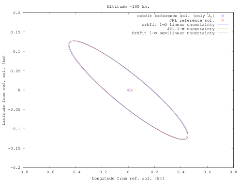
Figure 2: Nominal impact location and 1-$\sigma$ uncertainty region at 100 km altitude for 2008 TC₃. The linear uncertainty predictions by JPL and OrbFit, corresponding to the parameters of Table 1, are compared with the semilinear prediction.

In Figure 4 we show the 2008 TC₃ impact regions on ground and for altitudes corresponding to 37 km, 65.4 km and 100 km. Figure 4 is just an enlargement of Figure 4 between $h=37$ km and $h=0$ km. Detections of the actual atmospheric impact event suggested an atmospheric entry at 65.4 km, followed by an airburst explosion at an altitude of 37 km, with an energy equivalent to about one kiloton of TNT explosives. This explains why Figure 4 and Figure 4 also show the regions at altitudes 37 km and 65.4 km, in addition to those on the ground and at $h=100$ km. The blue line is the nominal ground track. Moreover, the locations of the recovered meteorites reported in Shaddad et al. (2010) are displayed, with larger and darker circles for larger masses. We show with different colours the different impact regions, according to the displayed legend. The south displacement of the smaller meteorites with respect to the predicted ground track is in agreement with the results of Farnocchia et al. (2017), where it is argued that the displacement is likely caused by winds.

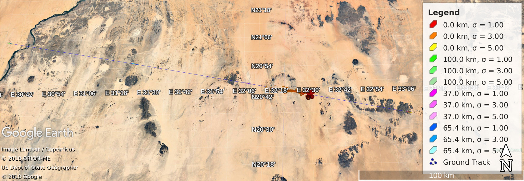
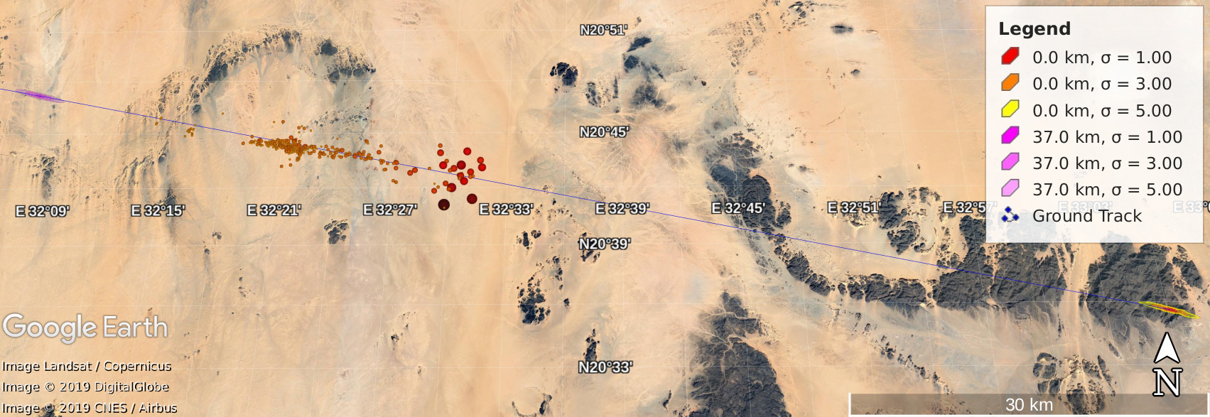
Figure 3: Prediction of the impact region of 2008 TC₃ with 883 observations.

Figure 4: Enlargement of Figure 4 between $h=37$ km and $h=0$ km.

In the second test we analysed the evolution of the impact corridor prediction, using different reduced observational data sets. For any selected batch of observations we performed the entire set of impact monitoring computations comprising the orbit determination, the impact prediction (VI search and characterisation), the IP computation and, as last step, the computation of the impact corridor. We selected as input the first 12, 16, and 26 observations, respectively. Even with so few observations the predicted IP reaches $1$. For any batch of observations we computed the impact regions at altitudes 100 and 0 km, for different confidence levels, namely $\sigma=1,3,5$. A Google Earth 3D visualisation of the impact regions is reported in Figure 6, 7 and 8.

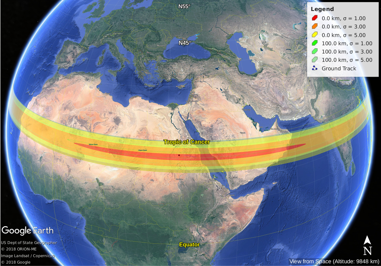
Figure 5: Prediction of the impact region of 2008 TC₃ using the first 12 observations (almost 18 hours before impact).

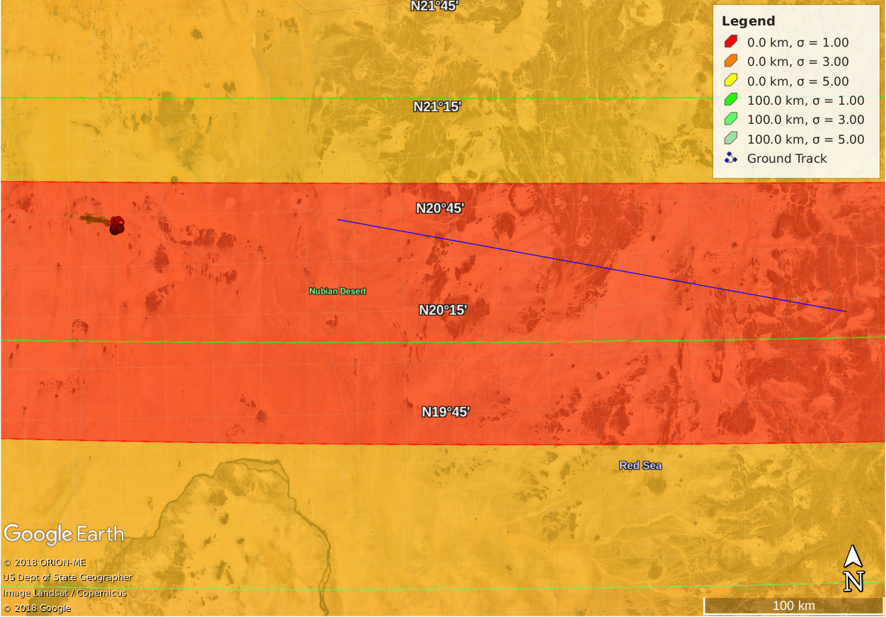
Figure 6: Enlargement of Figure 6, showing the ground track and the locations of the recovered meteorites.

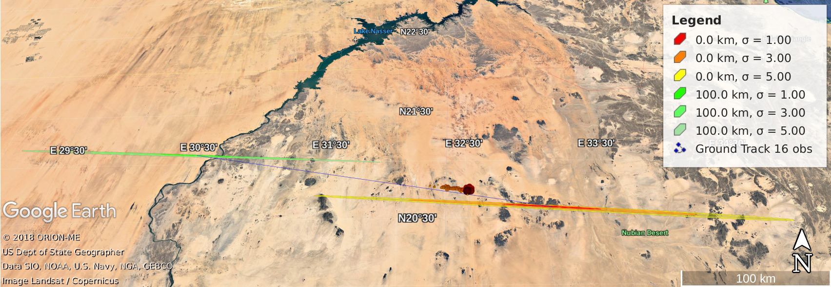
Figure 7: Prediction of the impact region of 2008 TC₃ using the first 16 observations (about 12 hours before impact).

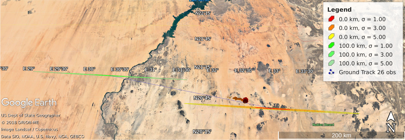
Figure 8: Prediction of the impact region of 2008 TC₃ using the first 26 observations (about 11 hours and a half before impact).

In the case with only 12 observations, represented in Figure 6, the uncertainty is still high, so that the impact region is very extended and surrounds the entire Earth. In this figure, the most part of the green regions at 100 km altitudes is not visible, because they overlap with the regions at 0 km altitude, that have the priority in the plot. Anyway, all the boundaries are visible. Moreover the ground track is far from the locations of the recovered meteorites. Nonetheless they are well inside the 1-$\sigma$ prediction, as it can be seen in the enlargement in Figure 6.

With 16 observations, the 1-$\sigma$ impact regions are about 70 km large. With 26 observations the 1-$\sigma$ impact regions size decreases to 40 km. For this cases the predicted ground track is near the locations of the recovered meteorites, even if they does not lie around it as it would be if the prediction was exact. Indeed, the ground track corresponding to 16 observations is shifted about half km southworth with respect to the ideal line crossing the middle of the meteorite locations. Surprisingly, the ground track corresponding to 26 observations is about 2 km farther toward South (see Figure 9). This causes a bigger part of the meteorites impact locations to be placed outside the 1-$\sigma$ impact corridor, whose approximated plot is obtained joining the semimajor axis endpoints at 100 and 0 km altitudes, see Figure 10 and 11.

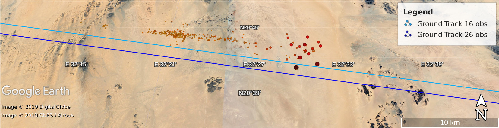
Figure 9: Ground tracks computed with 16 (light blue line) and 26 (blue line) observations, compared with the locations of the recovered 2008 TC₃ meteorites (red circles).

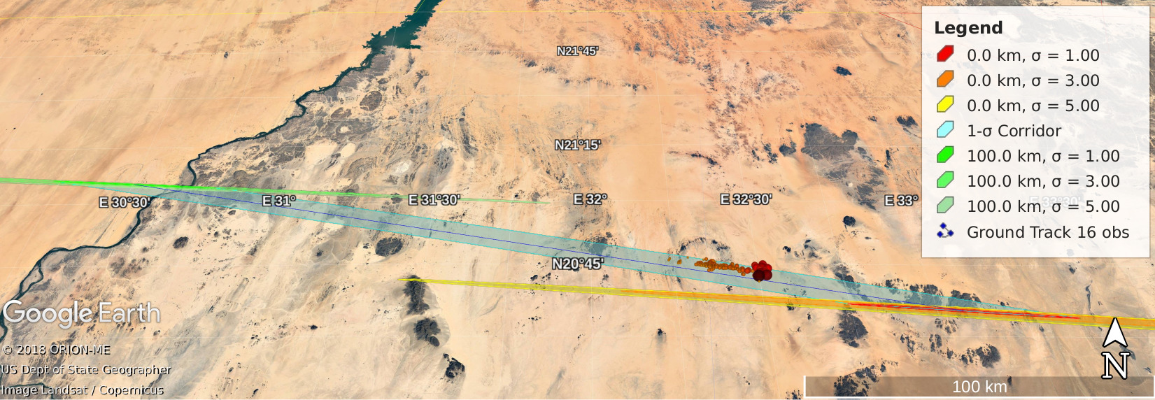
Figure 10: Approximated view of the 1-$\sigma$ impact corridor of 2008 TC₃ obtained with 16 observations.

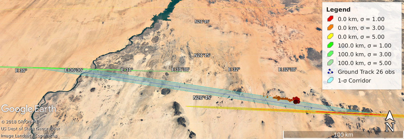
Figure 11: Approximated view of the 1-$\sigma$ impact corridor of 2008 TC₃ obtained with 26 observations.

From this second test it is clear that the impact region prediction, with whatever method, cannot bring to practical decisions, like for example the decision about to evacuate the region interested by a possible impact or even the selection of the place where to organise a mission for the recovery of meteorites after the impact occurred, when the uncertainty is too high. On the other hand, only by performing the prediction we have the precise measure of the size of the impact region on ground. In this particular test, only when at least 16 observations are available, we obtain a restricted impact area on ground.

6.2 2004 MN₄ - Apophis: Impact Prediction with 2004 Data

Apophis was first observed on June 19^th, 2004 by R. Tucker, D. Tholen and F. Bernardi from Kitt Peak over two consecutive nights. It was not observed for the following six months and it was recovered by chance on December 18^th by G. Garradd, who observed it for three consecutive nights. The object was recognised to be the one observed in June, with provisional designation 2004 MN₄, and the MPC released the new data of the recovered asteroid on December 20^th. With these data, both the clomon-2 a Sentry IM systems found the possibility of an impact in 2029. Anyway, due to some problems in the processing of the raw images, the reduced measurements of June were spoiled and consequently the fit showed very high residuals corresponding to those data. Consequently, the prediction of an impact was not trusted by the scientists, who asked for new data.

Already on December 23^rd, the availability of new observations and of the remeasurements of the bad June observations allowed the IM systems to provide a more reliable result. At this point, both clomon-2 and Sentry gave a VI in 2029 with Torino Scale Morrison et al. (2004); Binzel (2000) value 2 and Palermo Scale Chesley et al. (2002) greater than zero. The agreement between the systems was good and, even if the distribution and the quality of the observations was not optimal, the result was published. A note was added in the Risk Page, clarifying that this result was subject to change when new measurements would be available.

In the following days, after the addition of new incoming observations, the impact prediction continued to be confirmed and the impact probability grew to its maximum on December 27^th, when the IM systems gave $IP=0.027$ (1 in 38). A case like this had never happen before and, in addition to the near and high risk of impact, it presented new dynamical features which the clomon-2 software was not ready to deal with. It was a challenge for the NEODyS team to face the difficulties arising hour by hour, changing all the parts of the software that were not working properly in the minimum possible time.

The situation changed during the afternoon of December 27^th with the issue of 4 new special MPECs by the MPC. The last one, the MPEC-Y70, contained pre-discovery observations going back to March 2004. With those observations, the possibility of an impact in 2029 was ruled out during the night between December 27^th and 28^th, when the processing of the new data set was completed.

The details about the Apophis discovery and the story of the Apophis crisis following the prediction of an impact in 2029 can be found in Sansaturio and Arratia (2008). We recovered the situation for Apophis corresponding to December 27^th, 2004. The set of observations taken is the one of MPEC 2004-Y69. This set corresponds to the situation just before the availability of pre-discovery observations. Using OrbFit version 5.0, we computed a full least squares solution and we performed the impact monitoring with the options specified at the beginning of Section 6. The result of the IM gave a VI with impact on April 13^th, 2029 with probability $0.0242$ (1 in 41). The semilinear impact corridor was computed starting from this result, see top panel of Figure 12. The bottom panel of this figure shows the impact region computed with the same observational dataset by the JPL team using a Monte Carlo method. As it can be seen from the figures, there is a good agreement between the two independent predictions.

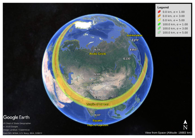
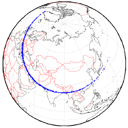
Figure 12: Top panel. Google Earth 3D visualisation of the semilinear prediction of the 2029 impact regions of Apophis, using the observations available on December 27^th, 2004 (MPEC 2004-Y69, 18:40 UT). Bottom panel. Monte Carlo prediction of the 2029 possible impact locations on ground of Apophis, using the same observational dataset of the above figure (JPL, private communication).

6.3 Impact Corridor for 2014 AA

Asteroid 2014 AA was discovered by R. Kowalski of the Catalina Sky Survey on January 1^st, 2014 at 06:18 UTC. The asteroid impacted the Earth on January 2^nd, 2014 at about 3 UTC, less than 21 hours after the first detection. The situation was similar to 2008 TC₃, but in this case very few observations were available before the impact, with a total of 7 optical measurements. Even with these few observations, the computed $IP$ was equal to $1$. The infrasonic airwaves produced by the 2014 AA atmospheric impact were detected by the infrasound component of the International Monitoring System operated by the Comprehensive Nuclear Test Ban Treaty Organization, as reported in Farnocchia et al. (2016).

We have applied the semilinear method using the impacting nominal solution as VI representative. In Figure 13, the semilinear impact regions on ground and at 100 km altitude are shown. The regions at the two altitudes almost overlap. This case is remarkable, because it is extremely non-linear, with the regions twisting on themselves. It follows that the coloured regions of the figure do not correspond to the interior of the regions delimited by the illustrated boundaries. The impact regions actually extend outside the drawn boundaries (the Jordan curve theorem does not apply because of the self-intersection of the non-linear image of the ellipse). This is confirmed by the fact that, in the vicinity of the torsion, the boundaries with lower $\sigma$ extends outside the ones with higher $\sigma$.

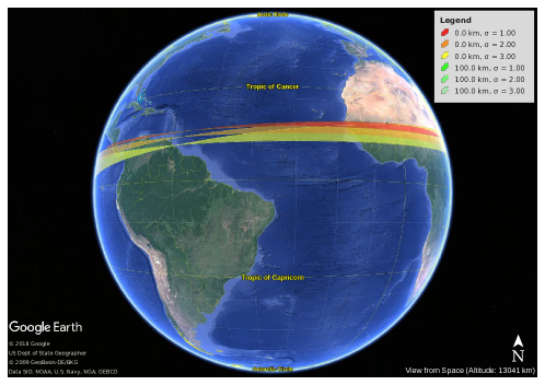
Figure 13: Google Earth 3D visualisation of 2014 AA impact regions for $\sigma$= 1, 2, 3 on ground and for 100 km altitude.

The region obtained by applying an observational Monte Carlo method is consistent with the boundaries obtained with the semilinear approach (see Figure 14), which confirms that the semilinear prediction is correct. The problem is that the boundaries given by the semilinear method in this case does not provide complete information on the impact region extension.

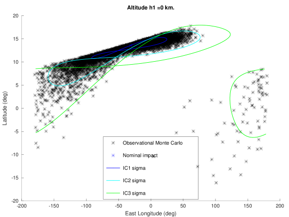
Figure 14: Comparison of the Monte Carlo prediction and the 2014 AA semilinear impact region boundaries on ground for $\sigma$= 1, 2, 3.

In conclusion, for cases like this one (the only one encountered so far, considering also other tests not reported here) the information provided by the semilinear boundary prediction is incomplete and can be misleading for a non-specialist audience.

6.4 Recent imminent impactors 2018 LA and 2019 MO

Object 2018 LA was a small (2-3 metres in diameter) Apollo near-Earth asteroid. It was discovered 8 hours before impact by the Mt. Lemmon Observatory of the Catalina Sky Survey. The impact occurred on June 2^nd, 2018 at 16:44 UTC (18:44 local time) in Botswana.

The orbit determination and IM computations were performed using all the available 14 observations and gave $IP=1$. The semilinear algorithm was used to compute the impact regions on ground corresponding to $\sigma=1,3,5$, which are shown in Figure 15 together with the firewall location, whose coordinates are extracted from the JPL fireballs web-page and reported in Table 2. As it can be seen from the figure, the fireball location is inside the 3-$\sigma$ prediction.

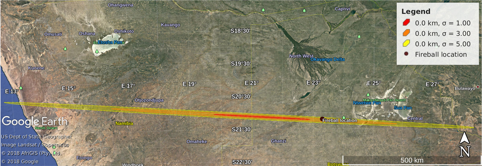
Figure 15: Google Earth 3D visualisation of 2018 LA impact regions on ground for $\sigma$= 1, 3, 5. The fireball location at 28.7 km altitude is also displayed.

Object 2019 MO was discovered from the ATLAS Mauna Loa observatory on June 22^nd, 2019 at 9:49 UTC. This object was a small (4-6 metres in diameter) Apollo near-Earth asteroid. It was discovered less than 12 hours before impact, which occurred on June 22^nd, 2019 at 21:25 UTC, between Jamaica and south American coast.

At the beginning, only four observations from the Mauna Loa site were available and the object was in the NEO Confirmation Page of the MPC, which contains unconfirmed objects. The Italian NEOScan Spoto et al. (2018) and the JPL Scout Farnocchia et al. (2015) systems routinely scan this page with the goal to find imminent impactors.

The object 2019 MO was indeed found to be an impactor by these systems, but with a low score, so that follow-up observations were not started promptly. Additional observations from the Pan-STARRS2 images were recovered only after the impact, on June 25^th. After this precovery, 7 observations were available and the fit was good enough to remove the object from the NEOCP and release an MPEC, but the object had already impacted the Earth. Anyway, post-impact computations were performed by the IM systems, giving an IP practically equal to 1 ($IP=0.994$ by clomon-2).

We computed the impact corridor for this object using the solution obtained with the entire set of 7 observations. The result is an impact region almost centred on the real impact location, which is known, because the fireball corresponding to the 2019 MO impact was observed. The semilinear impact region on ground and the fireball location at 25 km altitude are shown in Figure 16. The fireball data reported on the fireballs page of the JPL web-site are shown in Table 2.

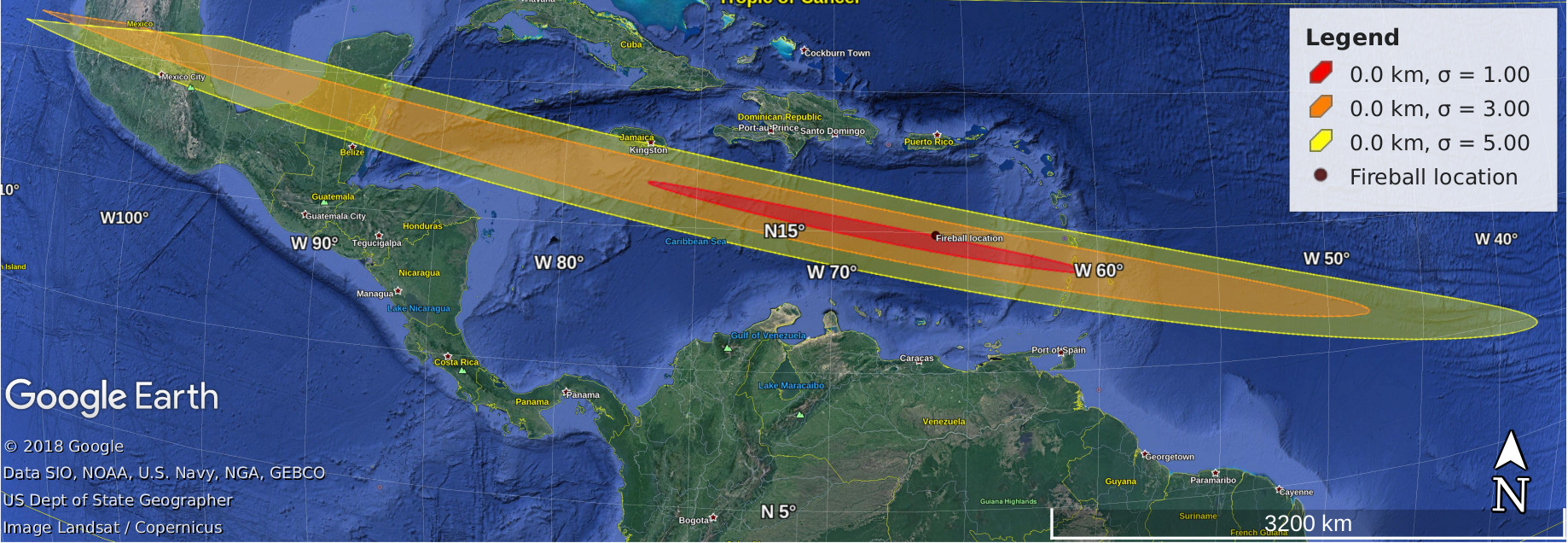
Figure 16: Google Earth 3D visualisation of 2019 MO impact regions on ground for $\sigma$= 1, 3, 5 and the fireball location at 25 km altitude.

Table 2: Fireball reports corresponding to 2018 LA and 2019 MO impacts, extracted from https://cneos.jpl.nasa.gov/fireballs/.

Peak Brightness Date/Time (UT)	Latitude (deg)	Longitude (deg)	Altitude (km)	Velocity (km/s)	Total Radiated Energy (J)	Calculated Total Impact Energy (kt)
2019-06-22 21:25:48	14.9N	66.2W	25.0	14.9	294.7e10	6
2018-06-02 16:44:12	21.2S	23.3E	28.7	16.9	37.5e10	0.98

As a final remark, we note that this kind of impact events occur quite frequently, but they are difficult to be predicted, because the objects are difficult to be observed before the impact. This case was the fourth after 2008 TC₃, 2014 AA and 2018 LA to be discovered just before the impact and having enough observations for a reliable orbit determination. Apart from 2014 AA, for all the other cases the semilinear algorithm succeeded in giving reliable predictions of the impact regions, even with few observations like 2019 MO.

7 Conclusions and future work

The semilinear method succeeds in providing the boundary of the impact region on ground, with a comparatively smaller number of propagations with respect to Monte Carlo approaches. Indeed, it samples a 1-dimensional curve instead of a region in the 6-dimensional orbital elements space.

It is possible to compute the impact probability associated with each boundary, absolute or conditional. For $IP=1$ it coincides with the probability of the orbital solution and is given by the level $\sigma$ of the considered impact region.

The algorithm has been tested using the real observations of the past impacted objects 2008 TC₃, 2014 AA, 2018 LA and 2019 MO. It has been applied also to the asteroid Apophis, but using only the observations available on December 27^th, 2004, before that pre-discovery observations were found. This situation corresponds to a possibility of impact in 2029 with probability of about 2.4%, as computed by the last version of OrbFit, version 5.0. For 2008 TC₃ and Apophis the predicted impact regions on ground are in good agreement with the Monte Carlo predictions by the JPL-NASA system. The semilinear prediction is especially good for 2008 TC₃, for which the predicted thin impact corridor along the ground track passes through the region of recovered meteorites. For 2018 LA and 2019 MO, the predicted semilinear impact regions contain the locations of the observed fireballs, even if very few observations are available. Only the case of 2014 AA reveals some limitations of the method. In this case the non-linearity causes the propagated uncertainty ellipse to twist on itself, so that the drawn boundary of the impact region does not encompass the inner points, and it provides incomplete and misleading information.

The performance of the implemented algorithm is good. It can be further improved using parallelisation. In particular, parallel computing is useful for special cases with low $IP$, near to the threshold of $10^{-3}$, with far impact time in the future and for which the implemented optimisation procedure cannot be applied, for example if there are multiple VIs with the same impact date. These cases correspond to a high level of non-linearity, but the semilinear prediction reveals to be still reliable. The only case in which the information provided could be misleading is when the effect of non-linearity is so high to cause a twist of the propagated uncertainty region, as it happens for the object 2014 AA. The best results in terms both of performance and accuracy are obtained for high impact probabilities and impact time near to the current date. It follows that the semilinear method is particularly useful for imminent impactors, as shown by the application of the method for the cases of the past impacted objects 2008 TC₃, 2018 LA and 2019 MO, for which the software takes between 30 and 50 seconds of runtime for each single impact region, with fixed altitude and $\sigma$, without the need of parallelisation.

The current software does not perform the computation of the IP associated with the impact regions. The current algorithm can be refined modifying the selection of the VI representative, in order to obtain a representative located as near as possible to the centre of the VI. This improvement is not straightforward. It requires a conversion of the LOV parameter to the corresponding physical distance along the LOV. Moreover, the case of a VI expanding off-LOV needs special attention.

A higher level improvement can be obtained combining together the semilinear method and the projection of the non-linear LOV on ground to obtain a more accurate prediction of the impact region.

References

- Binzel (2000) Binzel, R., 04 2000. The torino impact hazard scale. Planetary and Space Science 48, 297–303.
- Chesley et al. (2002) Chesley, S. R., Chodas, P. W., Milani, A., Valsecchi, G. B., Yeomans, D. K., October 2002. Quantifying the Risk Posed by Potential Earth Impacts. Icarus 159 (2), 423–432.
- Conte and de Boor (1980) Conte, S. D., de Boor, C., 1980. Elementary Numerical Analysis, Third Edition Edition. McGraw-Hill.
- Del Vigna (2018) Del Vigna, A., December 2018. On Impact Monitoring of Near-Earth Asteroids. Ph.D. thesis, Department of Mathematics at the University of Pisa.
- Del Vigna et al. (2018) Del Vigna, A., Faggioli, L., Spoto, F., Milani, A., Farnocchia, D., Carry, B., September 2018. Detecting the Yarkovsky effect among near-Earth asteroids from astrometric data. Astronomy & Astrophysics 617, A61.
- Del Vigna et al. (2020) Del Vigna, A., Guerra, F., Valsecchi, G. B., 2020. Improving impact monitoring through LOV densification. Icarus 351.
- Del Vigna et al. (2019) Del Vigna, A., Milani, A., Spoto, F., Chessa, A., Valsecchi, G. B., March 2019. Completeness of Impact Monitoring. Icarus 321, 647–660.
- Everhart (1985) Everhart, E., 1985. An Efficient Integrator that uses Gauss-Radau Spacings. International Astronomical Union Colloquium 83, 185–202.
- Farnocchia et al. (2016) Farnocchia, D., Chesley, S. R., Brown, P. G., Chodas, P. W., 2016. The trajectory and atmospheric impact of asteroid 2014 AA. Icarus 274, 327–333.
- Farnocchia et al. (2015) Farnocchia, D., Chesley, S. R., Chamberlin, A. B., Tholen, D. J., 2015. Star catalog position and proper motion corrections in asteroid astrometry. Icarus 245, 94–111.
- Farnocchia et al. (2015) Farnocchia, D., Chesley, S. R., Micheli, M., September 2015. Systematic ranging and late warning asteroid impacts. Icarus 258, 18–27.
- Farnocchia et al. (2017) Farnocchia, D., Jenniskens, P., Robertson, D. K., Chesley, S. R., Dimare, L., Chodas, P. W., 2017. The impact trajectory of asteroid 2008 TC3. Icarus 294, 218–226.
- Folkner et al. (2014) Folkner, W. M., Williams, J. G., Boggs, D. H., Park, R. S., Kuchynka, P., 2014. The Planetary and Lunar Ephemerides DE430 and DE431. The Interplanetary Network Progress Report 42-196, 1–81.
- Gauss (1809) Gauss, C. F., 1809. Theoria motus corporum coelestium in sectionis conicis solem ambientum. Hamburgi: sumtibus Frid. Perthes et I. H. Besser.
- Jordan (1887) Jordan, C., 1887. Cours d’Analyse de l’École Polytechnique. Vol. 3. Gauthier-Villars, Paris.
- Milani (1999) Milani, A., 1999. The Asteroid Identification Problem I. Recovery of Lost Asteroids. Icarus 137, 269–292.
- Milani et al. (2000) Milani, A., Chesley, S., Boattini, A., Valsecchi, G. B., 2000. Virtual impactors: search and destroy. Icarus 145 (1), 12–24.
- Milani et al. (2005a) Milani, A., Chesley, S. R., Sansaturio, M. E., Tommei, G., Valsecchi, G. B., 2005a. Nonlinear impact monitoring: line of variation searches for impactors. Icarus 173, 362–384.
- Milani and Gronchi (2010) Milani, A., Gronchi, G. F., 2010. Theory of orbit determination. Cambridge University Press.
- Milani et al. (2005b) Milani, A., Sansaturio, M. E., Tommei, G., Arratia, O., Chesley, S. R., 2005b. Multiple solutions for asteroid orbits: Computational procedure and applications. Astronomy & Astrophysics 431, 729–746.
- Milani and Valsecchi (1999) Milani, A., Valsecchi, G. B., 1999. The Asteroid Identification Problem II. Target Plane Confidence Boundaries. Icarus 140, 408–423.
- Morrison et al. (2004) Morrison, D., Chapman, C. R., Steel, D., P., B. R., 2004. Impacts and the Public: Communicating the Nature of the Impact Hazard. In: Belton, M. J. S., Morgan, T. H., Samarasinha, N. H., Yeomans, D. K. (Eds.), Mitigation of Hazardous Comets and Asteroids. Cambridge University Press.
- Moyer (2003) Moyer, T. D., 2003. Formulation for Observed and Computed Values of Deep Space Network Data Types for Navigation. Wiley-Interscience.
- NIMA - National Imagery and Mapping Agency (2000) NIMA - National Imagery and Mapping Agency, January 2000. Technical Report 8350.2 . Third Edition. Department of Defence World Geodetic System 1984. Its Definition and Relationships with Local Geodetic Systems. Tech. rep., NIMA - National Imagery and Mapping Agency.
- Sansaturio and Arratia (2008) Sansaturio, M. E., Arratia, O., June 2008. Apophis: the Story Behind the Scenes. Earth Moon and Planets 102 (1-4), 425–434.
- Shaddad et al. (2010) Shaddad, M. H., Jenniskens, P., Numan, D., Kudoda, A. M., Elsir, S., Riyad, I. F., Ali, A. E., Alameen, M., Alameen, N. M., Eid, O., Osman, A. T., Abubaker, M. I., Yousif, M., Chesley, S. R., Chodas, P. W., Albers, J., Edwards, W. N., Brown, P. G., Kuiper, J., Friedrich, J. M., 2010. The recovery of asteroid 2008 TC3. Meteoritics & Planetary Science 45 (10-11), 1557–1589.
- Spoto et al. (2018) Spoto, F., Del Vigna, A., Milani, A., Tommei, G., Tanga, P., Mignard, F., Carry, B., Thuillot, W., David, P., June 2018. Short arc orbit determination and imminent impactors in the Gaia era. Astronomy & Astrophysics 614, A27.
- Valsecchi et al. (2003) Valsecchi, G. B., Milani, A., Gronchi, G. F., Chesley, S. R., 2003. Resonant returns to close approaches: Analytical theory. Astronomy & Astrophysics 408, 1179–1196.