Thermodynamic Uncertainty Relations for Bosonic Otto Engines

Abstract

We study two-mode bosonic engines undergoing an Otto cycle. The energy exchange between the two bosonic systems is provided by a tunable unitary bilinear interaction in the mode operators modeling frequency conversion, whereas the cyclic operation is guaranteed by relaxation to two baths at different temperature after each interacting stage. By means of a two-point-measurement approach we provide the joint probability of the stochastic work and heat. We derive exact expressions for work and heat fluctuations, identities showing the interdependence among average extracted work, fluctuations and efficiency, along with thermodynamic uncertainty relations between the signal-to-noise ratio of observed work and heat and the entropy production. We outline how the presented approach can be suitably applied to derive thermodynamic uncertainty relations for quantum Otto engines with alternative unitary strokes.

I Introduction

Nonequilibrium processes are always accompanied by irreversible entropy production prig . When systems become smaller, as in nanoscopic heat engines nano1 ; nano2 , biological or chemical systems gnes ; rit ; rao or nanoelectronic devices ventra ; soth , the fluctuations of all thermodynamic quantities as work, heat, their correlations, and entropy production itself, become very relevant. For example, a macroscopic thermal engine supplies a certain amount of work while extracting heat from a hot thermal reservoir. As the thermodynamic machine size is reduced, the work output and heat absorbed are correspondingly scaled down, their fluctuations become more and more significant, and it becomes useful to investigate the stochastic properties of such fluctuating quantities.

A number of fluctuation theorems has been derived evans ; gal ; jar97 ; crook ; piecho ; jarz ; jarz3 ; seif2 ; marc ; saito ; andrie ; esp ; esp2 ; cth ; sini ; jarz2 ; camp ; seif ; frq ; hang ; esp3 as powerful relations that characterize the behavior of small systems out of equilibrium. Fluctuation relations pose stringent constraints on the statistics of fluctuating quantities as heat and work due to the symmetries (particularly, time-reversal symmetry) of the underlying microscopic dynamics. Furthermore, recent relations have also been developed, so called thermodynamic uncertainty relations (TUR), where the signal-to-noise ratio of observed work and heat has been related to the entropy production bar ; pietz ; ging2 ; pole ; pietz2 ; horo ; proes2 ; agar ; koy ; bar2 ; brad ; piet ; holu ; macie ; Li ; sary ; dech ; proes ; bar3 ; guar ; ging . Such TURs rule for example the tradeoff between entropy production and the output power relative fluctuations, i.e. the precision of a heat machine, so that working machines operating at near-to-zero entropy production cannot be achieved without a divergence in the relative output power fluctuations.

Although independently developed, fluctuation relations and TURs have been recently connected under various approaches and assumptions proes2 ; merh ; vanvu ; potts ; vanvu2 ; timpa ; zhang ; vanvu3 . In particular, in Ref. timpa a saturable TUR obtained from fluctuation theorems has been derived and compared with exact results pertaining to a microscopic two-qubit swap engine operating at the Otto efficiency.

In this paper we derive thermodynamic uncertainty relations for two-mode bosonic engines, where alternately each quantum harmonic oscillator is coupled to a thermal bath allowing heat exchange, and a unitary bilinear interaction determines energy exchange between the two modes by frequency conversion with tunable strength. We adopt the two-point-measurement scheme esp ; der ; th ; camp usually considered in the derivation of Jarzynski equality j97 and referred to the simultaneous estimation of both work and heat in order to derive the joint characteristic function that provides all moments of work and heat. The model is shown to achieve the Otto efficiency ot1 ; ot2 ; ot3 ; ot4 ; ot5 ; cpf ; dec ; ot6 , independently of the coupling parameter and the temperature of the reservoirs. After identifying the regimes where the periodic protocol works as a heat engine, a refrigerator, or a thermal accelerator, we provide the full joint probability of the stochastic work and heat in closed form.

Our derivation allows to obtain the exact relation between the signal-to-noise ratio of work and heat and the average entropy production of the engine, thus showing the deep interdependence among average extracted work, fluctuations, and entropy production. From these relations we derive thermodynamic uncertainty relations that are satisfied in all the regimes of operations and for any value of the bilinear coupling between the two quantum harmonic oscillators. A bound of the efficiency in terms of the average work and its fluctuations is also obtained.

As outlined in Appendix C, the presented approach can be applied to quantum thermodynamic engines with alternative unitary strokes in order to assess the validity of the standard TUR.

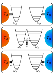
Figure 1: Two-mode bosonic Otto cycle in heat engine operation: in the first stage each quantum harmonic oscillator with frequency $\omega_{A}$ and $\omega_{B}$ is in thermal equilibrium with its respective bath at temperature $T_{A}$ and $T_{B}$, respectively, with $T_{A}>T_{B}$; in the second stage the two oscillators are isolated and let to interact by a bilinear unitary interaction ($\theta$), thus extracting work $W$; in the third stage the oscillators are let to relax to their respective thermal baths, thus absorbing heat $Q_{H}$ and releasing heat $Q_{C}$, such that the initial condition is reestablished. In the refrigeration regime all three arrows are reversed.

II The two-mode bosonic Otto engine

We illustrate now the two-mode bosonic engine under investigation, as depicted in Fig. 1. Let us fix natural units $\hbar=k_{B}=1$. Each system is described by bosonic mode operators $a,a^{\dagger}$ and $b,b^{{\dagger}}$, respectively, with the usual commutation relation, and corresponding free Hamiltonians $H_{A}=\omega_{A}\left(a^{{\dagger}}a+\frac{1}{2}\right)$ and $H_{B}=\omega_{B}\left(b^{{\dagger}}b+\frac{1}{2}\right)$. Initially, the two modes $a$ and $b$ are in thermal equilibrium with their own ideal bath at temperature $T_{A}$ and $T_{B}$, respectively, and we fix $T_{A}>T_{B}$. Hence, the initial state is characterized by the tensor product of bosonic Gibbs thermal states, i.e.

$$\rho_{0}=\frac{e^{-\beta_{A}H_{A}}}{Z_{A}}\otimes\frac{e^{-\beta_{B}H_{B}}}{Z_{B}}\;,$$ (1)

with $\beta_{X}=1/T_{X}$ and $Z_{X}=\operatorname{Tr}[e^{-\beta_{X}H_{X}}]$. The two systems are then isolated from their thermal baths and are allowed to interact via a global unitary transformation. We will consider the bilinear interaction that globally transforms the mode operators as follows

$$a^{\prime}=a\cos\theta+e^{i\varphi}b\sin\theta,$$ (2)

$$b^{\prime}=b\cos\theta-e^{-i\varphi}a\sin\theta,$$ (3)

with $\theta\in[0,\frac{\pi}{2}]$ and $\varphi\in[0,2\pi]$.

The Heisenberg transformations in Eqs. (2) and (3) correspond to a linear mixing of the modes that for $\omega_{A}\neq\omega_{B}$ describe frequency conversion, and in the Schrödinger picture are equivalent to the unitary transformation $U_{\xi}=\exp\left(\xi a^{{\dagger}}b-\xi^{*}ab^{{\dagger}}\right)$, with $\xi=\theta e^{i\varphi}$. We remark that $U_{\xi}$ incorporates the free evolutions, all interactions and classical external drivings, such that the corresponding unitary for the time-reversed process is just $U^{\dagger}_{\xi}$. We also notice that an extensive study of such thermodynamic coupling, especially for general Gaussian bipartite states, has been recently put forward in Ref. bil . In a quantum-optical scenario, this bilinear coupling may arise from an interaction Hamiltonian of duration $t$ between the couple of modes $a$ and $b$ and a third mode at frequency $|\omega_{A}-\omega_{B}|$ considered as a classical undepleted coherent pump with amplitude $\gamma$ via a nonlinear $\chi^{(2)}$ medium under parametric approximation mand ; par , such that in the interaction picture $\xi=\gamma\chi^{(2)}t$. In what follows the phase $\varphi$ is irrelevant, hence we pose $\varphi=0$.

After the interaction the two harmonic oscillators are reset to their equilibrium state of Eq. (1) via full thermalization by weak coupling to their respective baths. The procedure can be sequentially repeated and leads to a stroke engine. We notice that for $\theta=\pi/2$ the unitary $U_{\pi/2}$ performs a swap gate which exchanges the states of the two quantum systems, analogous to the two-qubit swap engine cpf ; timpa . More generally, here we consider an arbitrary value of $\theta$, modeling different interaction strengths (or times). In each cycle the energy change in mode $a$ due to the unitary stroke corresponds to the heat $Q_{H}$ released by the hot bath, i.e. $Q_{H}=-\Delta E_{a}$, and similarly we have $Q_{C}=-\Delta E_{b}$ for the heat dumped into the cold reservoir (heat is positive when it flows out of a reservoir). The work W is performed ($W>0$) or extracted ($W<0$) during the unitary interaction, and from the first law we have

$$W=-Q_{H}-Q_{C}=\Delta E_{a}+\Delta E_{b}\;.$$ (4)

We can characterize the engine by the independent random variables $W$ and $Q_{H}$, and study the characteristic function $\chi(\lambda,\mu)$, where $\lambda$ and $\mu$ denotes the work and heat labels such that all moments of work and heat can be obtained by the identity

$$\langle W^{n}Q_{H}^{m}\rangle=(-i)^{n+m}\left.\frac{\partial^{n+m}\chi(\lambda,\mu)}{\partial\lambda^{n}\partial\mu^{m}}\right|_{\lambda=\mu=0}\;.$$ (5)

The characteristic function depends on the procedure that is adopted to jointly estimate $W$ and $Q_{H}$. By using the two-point measurement scheme esp ; der ; th ; camp , we can write the characteristic function as follows camp

$$\chi(\lambda,\mu)=$$ (6)

$$\operatorname{Tr}[U^{\dagger}_{\theta}e^{-i\mu H_{A}}e^{i\lambda(H_{A}+H_{B})}U_{\theta}e^{i\mu H_{A}}e^{-i\lambda(H_{A}+H_{B})}\rho_{0}]\;.$$

By representing the thermal states as mixture of coherent states, namely

$$\frac{e^{-\beta_{X}H_{X}}}{Z_{X}}=\int\frac{d^{2}\gamma}{\pi N_{X}}e^{-\frac{|\gamma|^{2}}{N_{X}}}|\gamma\rangle\langle\gamma|\;,$$ (7)

with $d^{2}\gamma=d\mbox{Re}\gamma\;d\mbox{Im}\gamma$ and $N_{X}=(e^{\beta_{X}\omega_{X}}-1)^{-1}$, from the identities $e^{i\psi a^{\dagger}a}|\alpha\rangle=|\alpha e^{i\psi}\rangle$ and

$$U_{\theta}|\alpha\rangle|\delta\rangle=|\alpha\cos\theta+\delta\sin\theta\rangle|\delta\cos\theta-\alpha\sin\theta\rangle\;,$$ (8)

we have

$$\chi(\lambda,\mu)=\int\frac{d^{2}\alpha}{\pi N_{A}}\int\frac{d^{2}\gamma}{\pi N_{B}}e^{-\frac{|\alpha|^{2}}{N_{A}}-\frac{|\gamma|^{2}}{N_{B}}}$$ (9)

$$\times\langle\alpha\cos\theta+\gamma\sin\theta|\alpha\cos\theta+\gamma e^{i(\lambda-\mu)\omega_{A}-i\lambda\omega_{B}}\sin\theta\rangle$$

$$\times\langle\gamma\cos\theta-\alpha\sin\theta|\gamma\cos\theta-\alpha e^{i\lambda\omega_{B}-i(\lambda-\mu)\omega_{A}}\sin\theta\rangle\;.$$

Finally, from the relation

$$\langle\alpha|\gamma\rangle=\exp\left(-\frac{1}{2}|\alpha|^{2}-\frac{1}{2}|\gamma|^{2}+\bar{\alpha}\gamma\right)\;$$ (10)

and lengthy but straightforward Gaussian integration we obtain

$$\chi(\lambda,\mu)=\big{\{}1-\sin^{2}\theta\times$$ (11)

$$\left[(N_{A}+N_{B}+2N_{A}N_{B})[\cos(\mu\omega_{A}-\lambda(\omega_{A}-\omega_{B}))-1]\right.$$

$$\left.+i(N_{A}-N_{B})\sin(\mu\omega_{A}-\lambda(\omega_{A}-\omega_{B}))\right]\big{\}}^{-1}\;.$$

We easily check the identity $\chi[i\beta_{B},i(\beta_{B}-\beta_{A})]=1$, corresponding to the standard fluctuation theorem. Indeed, the time-reversal symmetry of the unitary operation provides the stronger identity $\chi[i\beta_{B}-\lambda,i(\beta_{B}-\beta_{A})-\mu]=\chi(\lambda,\mu)$, corresponding to the Gallavotti-Cohen microreversibility evans ; gal , and equivalent to the detailed fluctuation theorem andrie ; cth ; sini ; frq

$$\frac{p(W,Q_{H})}{p(-W,-Q_{H})}=e^{(\beta_{B}-\beta_{A})Q_{H}+\beta_{B}W}\;.$$ (12)

Notice the symmetry $\langle W^{n}Q_{H}^{m}\rangle=\left(\frac{\omega_{A}}{\omega_{B}-\omega_{A}}\right)^{m}\langle W^{n+m}\rangle$ and, from the first law, $\langle Q_{C}^{n}\rangle=(-\omega_{B}/\omega_{A})^{n}\langle Q_{H}^{n}\rangle$.

Using Eqs. (5) and (11) one obtains the following averages and variances of work and heat

$$\langle W\rangle=(\omega_{A}-\omega_{B})(N_{B}-N_{A})\sin^{2}\theta\;,$$ (13)

$$\langle Q_{H}\rangle=\omega_{A}(N_{A}-N_{B})\sin^{2}\theta=\frac{\omega_{A}}{\omega_{B}-\omega_{A}}\langle W\rangle\;,$$ (14)

$$\mbox{var}(W)=(\omega_{A}-\omega_{B})^{2}[N_{A}+N_{B}+2N_{A}N_{B}$$

$$\qquad\ \ \ +(N_{A}-N_{B})^{2}\sin^{2}\theta]\sin^{2}\theta\;,$$ (15)

$$\mbox{var}(Q_{H})=\frac{\omega^{2}_{A}}{(\omega_{A}-\omega_{B})^{2}}\mbox{var}(W)\;,$$ (16)

$$\mbox{cov}(W,Q_{H})=\frac{\omega_{A}}{\omega_{B}-\omega_{A}}\mbox{var}(W)\;.$$ (17)

We can identify three regimes of operation, namely

$$a) \ \ \ \omega_{A}>\omega_{B}\quad\&\quad N_{A}>N_{B}\qquad\quad\mbox{\ \ \ \ heat engine},$$

$$b) \ \ \ \omega_{A}>\omega_{B}\quad\&\quad N_{A}<N_{B}\qquad\quad\mbox{\ \ \ \ refrigerator},$$

$$c) \ \ \ \omega_{A}<\omega_{B}\quad(\implies N_{A}>N_{B})\ \ \ \ \mbox{thermal accelerator},$$

where correspondingly we have

$$a) \ \ \ \ \langle W\rangle<0,\qquad\langle Q_{H}\rangle>0,\qquad\langle Q_{C}\rangle<0\,;$$

$$b) \ \ \ \ \langle W\rangle>0,\qquad\langle Q_{H}\rangle<0,\qquad\langle Q_{C}\rangle>0\,;$$

$$c) \ \ \ \ \langle W\rangle>0,\qquad\langle Q_{H}\rangle>0,\qquad\langle Q_{C}\rangle<0\,.$$

We notice that for both the heat engine and the refrigerator the sign of $\mbox{cov}(W,Q_{H})$ is negative. On the other hand, for the thermal accelerator where external work is consumed to increase the heat flow from hot to cold reservoir the covariance is positive. In terms of the temperature of the reservoirs, it is useful to observe that

$$\beta_{A}\omega_{A}\leq\beta_{B}\omega_{B}\iff N_{A}\geq N_{B}\,,$$ (18)

and thus the three regimes are equivalently identified by

$$a)\ \ \frac{T_{B}}{T_{A}}<\frac{\omega_{B}}{\omega_{A}}<1;\ \ \ \ b)\ \ \frac{\omega_{B}}{\omega_{A}}<\frac{T_{B}}{T_{A}}<1;\ \ \ \ c)\ \frac{\omega_{B}}{\omega_{A}}>1.\;$$

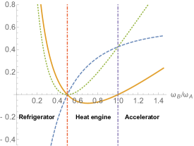
Figure 2: Plot of work, heat and entropy production (thick, dashed, and dotted style, respectively) for $\omega_{A}=1$, $\beta_{A}=1$, $\beta_{B}=2$, and $\theta=\pi/2$ versus the ratio $\omega_{B}/\omega_{A}$, in their three regions of operation.

The efficiency of the heat engine is given by

$$\eta=\frac{\langle-W\rangle}{\langle Q_{H}\rangle}=1-\frac{\omega_{B}}{\omega_{A}}\leq 1-\frac{T_{B}}{T_{A}}\equiv\eta_{C}\,,$$ (19)

corresponding to the Otto cycle efficiency. The Carnot efficiency $\eta_{C}$ is achieved only for $\omega_{A}/\omega_{B}=T_{A}/T_{B}$ (i.e., for $N_{A}=N_{B}$ with zero output work). Analogously, the coefficient of performance (COP) for the refrigerator is given by

$$\zeta=\frac{\langle Q_{C}\rangle}{\langle W\rangle}=\frac{\omega_{B}}{\omega_{A}-\omega_{B}}\leq\frac{T_{B}}{T_{A}-T_{B}}=\zeta_{C}\,.\;$$ (20)

Notice that both the efficiency and the COP are independent of $\theta$ and the temperature of the reservoirs.

Since $[U_{\theta},a^{\dagger}a+b^{\dagger}b]=0$ one has $\Delta E_{b}=-\frac{\omega_{B}}{\omega_{A}}\Delta E_{a}$, and hence the entropy production $\langle\Sigma\rangle$ can be written as follows

$$\langle\Sigma\rangle =\beta_{A}\Delta E_{a}+\beta_{B}\Delta E_{b}=\frac{\beta_{A}\omega_{A}-\beta_{B}\omega_{B}}{\omega_{A}-\omega_{B}}\langle W\rangle$$ (21)

$$=(\beta_{A}\omega_{A}-\beta_{B}\omega_{B})(N_{B}-N_{A})\sin^{2}\theta\;.$$

From Eq. (18), as expected, one always has $\langle\Sigma\rangle\geq 0$. Work, heat and entropy production are depicted in Fig. 2 for parameters $\omega_{A}=1$, $\beta_{A}=1$, and $\beta_{B}=2$, with $\theta=\pi/2$.

By the identity $\frac{\beta_{A}\omega_{A}-\beta_{B}\omega_{B}}{\omega_{A}-\omega_{B}}=-\frac{1}{T_{B}}(\frac{\eta_{C}}{\eta}-1)$, for the heat engine one obtains the relation

$$\langle\Sigma\rangle=\frac{\langle-W\rangle}{T_{B}}\left(\frac{\eta_{C}}{\eta}-1\right)\;$$ (22)

between average extracted work, entropy production and efficiency. Analogously, for the refrigerator one has

$$\langle\Sigma\rangle=\frac{\langle Q_{C}\rangle}{T_{A}}\left(\frac{1}{\zeta}-\frac{1}{\zeta_{C}}\right)\;.$$ (23)

III Thermodynamic uncertainty relations

Using Eqs. (11-15) one can obtain the inverse signal-to-noise ratios

$$\frac{\mbox{var}(W)}{\langle W\rangle^{2}} =\frac{\mbox{var}(Q_{H})}{\langle Q_{H}\rangle^{2}}=\frac{\mbox{cov}(W,Q_{H})}{\langle W\rangle\langle Q_{H}\rangle}$$ (24)

$$=\frac{N_{A}+N_{B}+2N_{A}N_{B}}{(N_{A}-N_{B})^{2}\sin^{2}\theta}+1\;.$$

These ratios are minimized versus $\theta$ for $\theta=\frac{\pi}{2}$, for which also the entropy production $\langle\Sigma\rangle$ achieves the maximum. Notice also that operating at zero entropy production (i.e. for $N_{A}\rightarrow N_{B}$, thus approaching the Carnot efficiency) will produce a divergence in Eq. (24). By combining Eqs. (21) and (24), independently of $\theta$ we obtain the following exact relation

$$\frac{\mbox{var}(W)}{\langle W\rangle^{2}}=\frac{h(\beta_{A}\omega_{A}-\beta_{B}\omega_{B})}{\langle\Sigma\rangle}+1\;,$$ (25)

where $h(x)=x\,\mbox{cth}(x/2)$. Then, reducing the noise-to-signal ratio associated to work extraction (or cooling performance) comes at a price of increased entropy production. Since $h(x)\geq 2$, the following thermodynamic uncertainty relation is always satisfied

$$\frac{\mbox{var}(W)}{\langle W\rangle^{2}}\geq\frac{2}{\langle\Sigma\rangle}+1\;,$$ (26)

and then also the standard TUR $\mbox{var}(W)/\langle W\rangle^{2}\geq 2/\langle\Sigma\rangle$.

In Fig. 3 we plot the work variance and compares it with the bound obtained by Eq. (26), for fixed parameters $\omega_{A}=1$, $\beta_{A}=1$, and $\beta_{B}=2$. Differently from the two-qubit case studied in Ref. timpa , we do not observe a violation of the standard TUR. Indeed, the tightest saturable bound from Ref. timpa

$$\frac{\mbox{var}(W)}{\langle W\rangle^{2}}\geq f(\langle\Sigma\rangle)\;,$$ (27)

where $f(x)=\mbox{csch}^{2}[g(x/2)]$ and $g(x)$ denotes the inverse function of $x\,\mbox{tanh}(x)$, becomes quite loose for the present bosonic engine for $\omega_{B}\ll\omega_{A}$ (see Fig. 3). For a more direct comparison with the two-qubit engine, where the standard TUR can be violated, see Appendix A. The effect of finite thermalization times on the TUR is also considered in Appendix D.

From Eqs. (22) and (26) we can write a relation between the average extracted work, fluctuations and efficiency

$$\langle-W\rangle\leq\frac{\mbox{var}(W)}{2T_{B}}\left(\frac{\eta_{C}}{\eta}-1\right)\;.$$ (28)

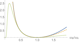
Figure 3: Plot of the work variance $\mbox{var}(W)$ (thick style) and the function $\langle W\rangle^{2}\left(\frac{2}{\langle\Sigma\rangle}+1\right)$ in dashed style, for $\omega_{A}=1$, $\beta_{A}=1$, and $\beta_{B}=2$ versus the ratio $\omega_{B}/\omega_{A}$. The dotted curve is obtained by the lower bound in Eq. (27) derived in Ref. timpa .

This can also be written as a bound on the efficiency, determined by the average work and fluctuations, namely

$$\eta\leq\frac{\eta_{C}}{1+2T_{B}\langle-W\rangle/\mbox{var}(W)}\;.$$ (29)

We notice that Eqs. (28) and (29) are analogous to the universal trade-off derived in Ref. piet for steady-state engines permanently coupled to heat baths. The bound (29) shows that in order to increase the efficiency, one must either sacrifice the output work or increase the fluctuations, thus decreasing the engine reliability.

We observe that both the stochastic work and heat come as integer multiple of $\omega_{A}-\omega_{B}$ and $\omega_{A}$, respectively. In fact, this can also be understood luk ; sele by noting that the characteristic function has periodicity $\frac{2\pi}{|\omega_{A}-\omega_{B}|}$ and $\frac{2\pi}{\omega_{A}}$ in the variables $\lambda$ and $\mu$. The joint probability for work and heat is then given by

$$\!\!p[W=m(\omega_{A}-\omega_{B}),Q_{H}=n\omega_{A}]=\frac{\omega_{A}|\omega_{A}-\omega_{B}|}{(2\pi)^{2}}$$ (30)

$$\!\!\!\!\times\int_{-\frac{\pi}{|\omega_{A}-\omega_{B}|}}^{\frac{\pi}{|\omega_{A}-\omega_{B}|}}d\lambda\int_{-\frac{\pi}{\omega_{A}}}^{\frac{\pi}{\omega_{A}}}d\mu\,\chi(\lambda,\mu)e^{-i\lambda m(\omega_{A}-\omega_{B})-i\mu n\omega_{A}}$$

$$\!\!\!\!=p[W=m(\omega_{A}-\omega_{B})]\delta_{n,-m}=p[Q_{H}=n\omega_{A}]\delta_{m,-n}\;,$$

where, by the derivation given in Appendix B,

$$p[Q_{H}=n\omega_{A}]=p[W=-n(\omega_{A}-\omega_{B})]=\frac{1}{\sqrt{1+2(N_{A}+N_{B}+2N_{A}N_{B})\sin^{2}\theta+(N_{A}-N_{B})^{2}\sin^{4}\theta}}$$ (31)

$$\times\left\{\begin{array}[]{ll}\left(\frac{1+(N_{A}+N_{B}+2N_{A}N_{B})\sin^{2}\theta-\sqrt{1+2(N_{A}+N_{B}+2N_{A}N_{B})\sin^{2}\theta+(N_{A}-N_{B})^{2}\sin^{4}\theta}}{2N_{B}(N_{A}+1)\sin^{2}\theta}\right)^{n}&\qquad\mbox{for }n\geq 0\;,\\ \left(\frac{1+(N_{A}+N_{B}+2N_{A}N_{B})\sin^{2}\theta-\sqrt{1+2(N_{A}+N_{B}+2N_{A}N_{B})\sin^{2}\theta+(N_{A}-N_{B})^{2}\sin^{4}\theta}}{2N_{A}(N_{B}+1)\sin^{2}\theta}\right)^{|n|}&\qquad\mbox{for }n<0\;.\end{array}\right.\;$$ (34)

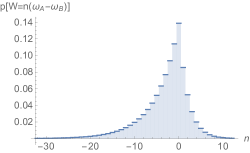
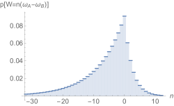
Figure 4: Distribution of the extracted work in $\omega_{A}-\omega_{B}$ units, for $N_{A}=8$ and $N_{B}=2$, for interaction strength $\theta=\pi/4$ (left) and $\theta=\pi/2$ (right). By exchanging $n\rightarrow-n$, the same histograms represent the probability of heat released by the hotter reservoir in $\omega_{A}$ units [see Eq. (31) and (B7)].

In Fig. 4 we report the work probability for $N_{A}=8$ and $N_{B}=2$, pertaining to two different values of strength interaction, i.e. $\theta=\pi/4$ and $\theta=\pi/2$.

From the form of Eq. (30), similarly to the case of the two-qubit swap engine cpf , one recognizes that the efficiency is indeed a self-averaging quantity. In fact, in principle the efficiency $\eta=\frac{\langle-W\rangle}{\langle Q_{H}\rangle}$ is different from the expectation of the stochastic efficiency $\eta_{s}=\langle-W/Q_{H}\rangle$. However, here we have for all moments

$$\langle(-W/Q_{H})^{n}\rangle=\langle-W/Q_{H}\rangle^{n}=\left(1-\frac{\omega_{B}}{\omega_{A}}\right)^{n}\;,$$ (35)

namely there are no efficiency fluctuations.

The closed form for the probability of Eq. (31) allows one to explicitly verify the detailed fluctuation theorem in Eq. (12) as follows

$$\frac{p[W=-n(\omega_{A}-\omega_{B}),Q_{H}=n\omega_{A}]}{p[W=n(\omega_{A}-\omega_{B}),Q_{H}=-n\omega_{A}]}=\left[\frac{N_{A}(N_{B}+1)}{N_{B}(N_{A}+1)}\right]^{n}$$

$$=e^{(\beta_{B}-\beta_{A})n\omega_{A}-\beta_{B}n(\omega_{A}-\omega_{B})}=e^{(\beta_{B}-\beta_{A})Q_{H}+\beta_{B}W}\;.$$ (36)

In Appendix C we provide a general discussion on the special character of the joint probability $p(W,Q_{H})$ and the outline of the generalization of the present approach to study Otto engines with alternative unitary interactions.

IV Conclusions

In conclusion, by adopting the two-point-measurement protocol for the joint estimation of work and heat, we have derived exact expressions for work and heat fluctuations pertaining to two-mode bosonic Otto engines, where two quantum harmonic oscillators are alternately subject to a tunable unitary bilinear interaction and to thermal relaxation to their own reservoirs. We have derived the characteristic function for work and heat, and obtained the full joint probability of the stochastic work and heat.

The presented thermodynamic uncertainty relations show the interdependence among average extracted work, fluctuations and entropy production, which hold in all range of coupling parameter between the two quantum harmonic oscillators. Our results confirm the general meaning of TURs, namely that reducing the noise-to-signal ratio associated with a given current comes at a price of increased entropy production.

The direct derivation of TURs by explicit measurement protocols can be effective in a variety of stroke thermodynamic engines. Within this approach, the relevance of the algebraic properties of the interactions naturally emerges.

The connection between fluctuation theorems, estimation protocols and thermodynamic uncertainty relations represents a significant advance in our understanding of nonequilibrium phenomena, and is relevant for the design of quantum thermodynamic machines, by posing strict bounds that relate work, heat, fluctuations, efficiency, and reliability.

Appendix A a comparison with the two-qubit Otto engine

It is interesting to compare the results for the two-mode bosonic Otto engine with the case of the two-qubit Otto engine. Hence, we extend the study of Ref. timpa to the case of partial swap, by considering a two-qubit unitary interaction

$$U_{\theta}=\left(\begin{array}[]{cccc}1&0&0&0\\ 0&\cos\theta&\sin\theta&0\\ 0&-\sin\theta&\cos\theta&0\\ 0&0&0&1\end{array}\right)\;,$$ (41)

where we used the tensor-product ordered basis $|00\rangle,|01\rangle,|10\rangle,|11\rangle$ for two qubits. The characteristic function is still obtained by Eq. (6) of the main text, where now $H_{X}=-\omega_{X}|0\rangle\langle 0|$. A simple calculation gives

$$\chi(\lambda,\mu)=1+$$

$$\sin^{2}\theta\{(N_{A}+N_{B}-2N_{A}N_{B})[\cos(\mu\omega_{A}-\lambda(\omega_{A}-\omega_{B}))-1]+i(N_{A}-N_{B})[\sin(\mu\omega_{A}-\lambda(\omega_{A}-\omega_{B}))]\}\;,$$ (42)

where now $N_{X}=(e^{\beta_{X}\omega_{X}}+1)^{-1}$. The odd and even moments are given by

$$\langle Q_{H}^{2n+1}\rangle=\omega_{A}^{2n+1}(N_{A}-N_{B})\sin^{2}\theta\;,$$ (43)

$$\langle Q_{H}^{2n}\rangle=\omega_{A}^{2n}(N_{A}+N_{B}-2N_{A}N_{B})\sin^{2}\theta\;,$$ (44)

and $\langle W^{n}Q_{H}^{m}\rangle=\left(\frac{\omega_{B}-\omega_{A}}{\omega_{A}}\right)^{n}\langle Q_{H}^{n+m}\rangle$. The entropy production has the same formal expression of the bosonic case, namely

$$\langle\Sigma\rangle=(\beta_{A}\omega_{A}-\beta_{B}\omega_{B})(N_{B}-N_{A})\sin^{2}\theta\;,$$ (45)

whereas the inverse signal-to-noise ratios reads

$$\frac{\mbox{var}(W)}{\langle W\rangle^{2}}=\frac{\mbox{var}(Q_{H})}{\langle Q_{H}\rangle^{2}}=\frac{N_{A}+N_{B}-2N_{A}N_{B}}{(N_{A}-N_{B})^{2}\sin^{2}\theta}-1\;.$$ (46)

For the qubit engine, Eq. (25) of the main text is then replaced with

$$\frac{\mbox{var}(W)}{\langle W\rangle^{2}}=\frac{h(\beta_{A}\omega_{A}-\beta_{B}\omega_{B})}{\langle\Sigma\rangle}-1\;,$$ (47)

where, remarkably, the same function $h(x)=x\,\mbox{cth}(x/2)$ appears. Since around the affinity $x=\beta_{A}\omega_{A}-\beta_{B}\omega_{B}$ one has $2\leq h(x)\leq 2+\frac{x^{2}}{6}$ the standard TUR

$$\frac{\mbox{var}(W)}{\langle W\rangle^{2}}\geq\frac{2}{\langle\Sigma\rangle}\;$$ (48)

can be tinily violated for the qubit engine, as shown in Ref. timpa . In Fig. 5 we report the signal-to-noise ratio $\langle W\rangle^{2}/\mbox{var}(W)$ along with the function $\langle\Sigma\rangle/2$ for the cases $\theta=\pi/2$ and $\theta=\pi/3$. We observe that the region of violation of the thermodynamic uncertainty relation (48) is shrunk for decreasing values of $\theta$.

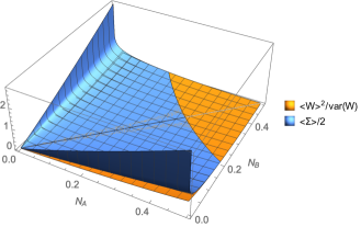
Figure 5: Plot of the signal-to-noise ratio of work $\langle W\rangle^{2}/\mbox{var}(W)$ and scaled entropy production $\langle\Sigma\rangle/2$ for the qubit Otto engine with $\theta=\pi/2$ (left) and $\theta=\pi/3$ (right) as a function of parameters $N_{A}$ and $N_{B}$.

For the qubit engine the probability for the stochastic heat and work has finite outcomes and is obtained as follows

$$p[Q_{H}=n\omega_{A}]=p[W=-n(\omega_{A}-\omega_{B})]$$

$$=\frac{1}{2\pi}\int_{0}^{2\pi}\left\{1+\sin^{2}\theta\left[(N_{A}+N_{B}-2N_{A}N_{B})[(\cos\mu)-1]+i(N_{A}-N_{B})\sin\mu\right]\right\}\,e^{-i\mu n}\,d\mu$$

$$=\left\{\begin{array}[]{ll}1-(N_{A}+N_{B}-2N_{A}N_{B})\sin^{2}\theta&\qquad\mbox{for }n=0\;,\\ N_{A}(1-N_{B})\sin^{2}\theta&\qquad\mbox{for }n=1\;,\\ N_{B}(1-N_{A})\sin^{2}\theta&\qquad\mbox{for }n=-1\;.\\ \end{array}\right.\;$$ (52)

As we have shown above, this three-point probability may give rise to a violation of Eq. (48). The finiteness of the stochastic outcomes and the different algebra of operators concur to provide a different thermodynamic uncertainty relation with respect to the bosonic case. We recall that the saturable bound of the main text (27) provides a stronger violation of the standard TUR and is achieved by a two-point distribution, as shown in Ref. timpa .

Appendix B probability for the stochastic work and heat of the bosonic Otto engine

From the Eq. (30) of the main text, in order to obtain the probability for the stochastic work and heat we need to perform the following integral

$$p[Q_{H}=n\omega_{A}] =p[W=-n(\omega_{A}-\omega_{B})]$$

$$=\frac{1}{2\pi}\int_{0}^{2\pi}\big{\{}1-\left[(N_{A}+N_{B}+2N_{A}N_{B})[(\cos\mu)-1]+i(N_{A}-N_{B})\sin\mu\right]\sin^{2}\theta\big{\}}^{-1}e^{-i\mu n}d\mu\;.$$

The integral can be solved by using the residue theorem, after posing $z=e^{i\mu}$ and integrating on the complex plane along the unit circle $\gamma$, with $d\mu=dz/(iz)$. Then, we have

$$p[Q_{H}=n\omega_{A}] =\frac{1}{2\pi}\int_{\gamma}\big{\{}1-\left[(N_{A}+N_{B}+2N_{A}N_{B})[(z+z^{-1})/2-1]+i(N_{A}-N_{B})(z-z^{-1})/(2i)\right]\sin^{2}\theta\big{\}}^{-1}z^{-n}\frac{dz}{iz}$$ (54)

$$=\frac{1}{2\pi i}\int_{\gamma}\frac{z^{-n}}{[1+(N_{A}+N_{B}+2N_{A}N_{B})\sin^{2}\theta]z-[N_{A}(N_{B}+1)z^{2}+N_{B}(N_{A}+1)]\sin^{2}\theta}dz\;.$$

For $n\leq 0$ the poles are easily evaluated as

$$z_{\pm}=\frac{1+(N_{A}+N_{B}+2N_{A}N_{B})\sin^{2}\theta\pm\sqrt{1+2(N_{A}+N_{B}+2N_{A}N_{B})\sin^{2}\theta+(N_{A}-N_{B})^{2}\sin^{4}\theta}}{2N_{A}(N_{B}+1)\sin^{2}\theta}\;.$$ (55)

We observe that

$$z_{+}>\frac{1+[(N_{A}+N_{B}+2N_{A}N_{B})+|N_{A}-N_{B}|]\sin^{2}\theta}{2N_{A}(N_{B}+1)\sin^{2}\theta}\;.$$ (56)

Then, for $N_{A}\geq N_{B}$ clearly one has $z_{+}>1$. For $N_{A}<N_{B}$, one also has

$$z_{+}>\frac{1+2N_{B}(N_{A}+1)\sin^{2}\theta}{2N_{A}(N_{B}+1)\sin^{2}\theta}>1\;,\;$$ (57)

since $N_{B}>N_{A}>0\iff N_{B}(N_{A}+1)>N_{A}(N_{B}+1)$. Hence, the pole $z_{+}$ lies outside the unitary circle.

The residue for the first-order pole $z_{-}$ is given by

$$\mbox{Res}\left(\frac{z^{|n|}}{[1+(N_{A}+N_{B}+2N_{A}N_{B})\sin^{2}\theta]z-[N_{A}(N_{B}+1)z^{2}+N_{B}(N_{A}+1)]\sin^{2}\theta},z_{-}\right)$$

$$=\left.\frac{z^{|n|}}{[1+(N_{A}+N_{B}+2N_{A}N_{B})\sin^{2}\theta]-2N_{A}(N_{B}+1)z\sin^{2}\theta}\right|_{z=z_{-}}$$

$$=\frac{1}{\sqrt{1+2(N_{A}+N_{B}+2N_{A}N_{B})\sin^{2}\theta+(N_{A}-N_{B})^{2}\sin^{4}\theta}}$$

$$\times\left(\frac{1+(N_{A}+N_{B}+2N_{A}N_{B})\sin^{2}\theta-\sqrt{1+2(N_{A}+N_{B}+2N_{A}N_{B})\sin^{2}\theta+(N_{A}-N_{B})^{2}\sin^{4}\theta}}{2N_{A}(N_{B}+1)\sin^{2}\theta}\right)^{|n|}\;$$ (58)

For $n>0$, we also have a $n$-order pole in $z=0$. However, we can recast the integration as for the case $n<0$ by the change of variable $\mu\rightarrow-\mu$, which is then equivalent to exchange $N_{A}$ with $N_{B}$. Hence, one obtains the closed expression for the probability for the stochastic work and heat of Eq. (31).

In the case of the swap engine $\theta=\frac{\pi}{2}$, one can directly derive the analytic expression for $p[Q_{H}=n\omega_{A}]$ as follows

$$p[Q_{H}=n\omega_{A}]=p[W=-n(\omega_{A}-\omega_{B})]=\sum_{l,s=0}^{\infty}\operatorname{Tr}[(|l\rangle\langle l|\otimes I_{B})U_{\pi/2}(|s\rangle\langle s|\otimes\rho_{N_{B}})U^{\dagger}_{\pi/2}]\langle s|\rho_{N_{A}}|s\rangle\,\delta_{n,s-l}$$

$$=\sum_{l,s=0}^{\infty}\frac{1}{N_{A}+1}\left(\frac{N_{A}}{N_{A}+1}\right)^{s}\frac{1}{N_{B}+1}\left(\frac{N_{B}}{N_{B}+1}\right)^{l}\delta_{n,s-l}=\left\{\begin{array}[]{ll}\frac{1}{1+N_{A}+N_{B}}\left(\frac{N_{A}}{N_{A}+1}\right)^{n}&\qquad\mbox{for }n\geq 0\;,\\ \frac{1}{1+N_{A}+N_{B}}\left(\frac{N_{B}}{N_{B}+1}\right)^{|n|}&\qquad\mbox{for }n<0\;,\end{array}\right.$$ (61)

consistent with Eq. (31) for $\theta=\frac{\pi}{2}$.

Appendix C general consideration on the joint probability $p(W,Q_{H})$.

We would like to make some general considerations about the special character of the joint probability $p(W,Q_{H})$. Let us come back to the characteristic function $\chi(\lambda,\mu)$ in Eq. (6) of the main text. We notice that the periodicity in $\lambda$ and $\mu$ which is evident in Eq. (11) can be indeed recognized from the expression of Eq. (6) without explicit calculation, but exploiting the algebra of bosonic operators, since one can rewrite

$$\chi(\lambda,\mu)=\operatorname{Tr}[U^{\dagger}_{\theta}U_{\xi}\rho_{0}]\;,$$ (62)

where $\xi=\theta e^{i\lambda(\omega_{A}-\omega_{B})-i\mu\omega_{A}}$. The fact that $\chi(\lambda,\mu)$ is a function of the single variable $\lambda(\omega_{A}-\omega_{B})-\mu\omega_{A}$ is due to the symmetry $[U_{\theta},a^{\dagger}a+b^{\dagger}b]=0$, and from this the Kronecker delta is obtained as

$$p[W=m(\omega_{A}-\omega_{B}),Q_{H}=n\omega_{A}] =\frac{\omega_{A}|\omega_{A}-\omega_{B}|}{(2\pi)^{2}}\int_{-\frac{\pi}{|\omega_{A}-\omega_{B}|}}^{\frac{\pi}{|\omega_{A}-\omega_{B}|}}d\lambda\int_{-\frac{\pi}{\omega_{A}}}^{\frac{\pi}{\omega_{A}}}d\mu\,\chi(\lambda,\mu)e^{-i\lambda m(\omega_{A}-\omega_{B})-i\mu n\omega_{A}}$$ (63)

$$=\delta_{m,-n}\,\frac{1}{2\pi}\int_{0}^{2\pi}\chi\left(0,\frac{\mu}{\omega_{A}}\right)e^{-i\mu n}d\mu\;.$$

This feature can also be obtained in other thermodynamic engines where a different observable is a constant of motion during the unitary strokes. For example, one can consider the unitary $V_{\theta}=\exp(\theta a^{\dagger}b^{2}-\theta^{*}ab^{{\dagger}2})$, where now the constant of motion is $2a^{\dagger}a+b^{\dagger}b$. The characteristic function is then given by $\chi(\lambda,\mu)=\operatorname{Tr}[V^{\dagger}_{\theta}V_{\zeta}\rho_{0}]$ with $\zeta=\theta e^{i\lambda(\omega_{A}-2\omega_{B})-i\mu\omega_{A}}$, and hence

$$p[W=m(\omega_{A}-2\omega_{B}),Q_{H}=n\omega_{A}]=p[W=m(\omega_{A}-2\omega_{B})]\delta_{n,-m}=p[Q_{H}=n\omega_{A}]\delta_{m,-n}\;.$$ (64)

Clearly, also in this case the efficiency $\eta=\langle-W/Q_{H}\rangle=1-2\omega_{B}/\omega_{A}$ has no fluctuations. Even without finding explicitly the stochastic distribution one can exploit this result for proving some thermodynamic properties. For example, in this case we can write the average entropy production as follows

$$\langle\Sigma\rangle=-\frac{\beta_{A}\omega_{A}-2\omega_{B}\beta_{B}}{\omega_{A}}\langle Q_{H}\rangle=\frac{\beta_{A}\omega_{A}-2\omega_{B}\beta_{B}}{\omega_{A}-2\omega_{B}}\langle W\rangle\;.$$ (65)

By requiring the positivity of the entropy production one can easily infer the condition for having a heat-engine operation $\langle Q_{H}\rangle>0$ and $\langle W\rangle<0$, namely $\beta_{A}\omega_{A}<2\beta_{B}\omega_{B}$ and $\omega_{A}>2\omega_{B}$. We notice that the first of these conditions is equivalent to $N_{A}>N_{B}^{2}/(2N_{B}+1)$. Further work is required in order to obtain other properties related to higher moments (e.g. thermodynamic uncertainty relations), since the algebra of operators $(a^{\dagger}b^{2},ab^{{\dagger}2},a^{\dagger}a,b^{\dagger}b)$ is not closed. The presented approach might be fruitful for the study of nonlinear optical interactions from a thermodynamic perspective.

Similarly, for the two-mode squeezing unitary interaction $S_{r}=\exp[r(a^{\dagger}b^{\dagger}-ab)]$ for which $[S_{r},a^{\dagger}a-b^{\dagger}b]=0$, one obtains

$$p[W=m(\omega_{A}+\omega_{B}),Q_{H}=n\omega_{A}]=p[W=m(\omega_{A}+\omega_{B})]\delta_{n,-m}=p[Q_{H}=n\omega_{A}]\delta_{m,-n}\;.$$ (66)

In this case the engine can work just as a dud machine, since one always has $\langle W\rangle\geq 0$, along with $\langle Q_{H}\rangle,\langle Q_{C}\rangle\leq 0$. Basically, in this case the unitary strokes perform work $W=(\omega_{A}+\omega_{B})(N_{A}+N_{B}+1)\sinh^{2}r$ to build correlations that are then converted to heat when the two harmonic oscillators relax to equilibrium by their thermal reservoirs. This is consistent with a general result obtained in Ref. bil , where it is shown that the presence of initial correlations is needed to extract work by the interaction $S_{r}$. By exploiting the closed algebraic transformations

$$S^{\dagger}_{r}aS_{r}=a\cosh r+b^{\dagger}\sinh r,$$ (67)

$$S^{\dagger}_{r}bS_{r}=b\cosh r+a^{\dagger}\sinh r,$$ (68)

from the general formula of the main text (5) one obtains

$$\langle W\rangle=(\omega_{A}+\omega_{B})(N_{A}+N_{B}+1)\sinh^{2}r\;,$$

$$\frac{\mbox{var}(W)}{\langle W\rangle^{2}}=\frac{N_{A}+N_{B}+2N_{A}N_{B}+1}{(N_{A}+N_{B}+1)^{2}\sinh^{2}r}+1\,.$$ (69)

The entropy production reads

$$\langle\Sigma\rangle=\frac{\beta_{A}\omega_{A}+\beta_{B}\omega_{B}}{\omega_{A}+\omega_{B}}\langle W\rangle\;,$$ (70)

and hence, for any value of the interaction strength $r$, one obtains the exact relation

$$\frac{\mbox{var}(W)}{\langle W\rangle^{2}}=\frac{h(\beta_{A}\omega_{A}+\beta_{B}\omega_{B})}{\langle\Sigma\rangle}+1\;.$$ (71)

Remarkably, as for the interaction $U_{\theta}$, the function $h(x)=x\,\mbox{cth}(x/2)$ appears, and then also in this case the thermodynamic uncertainty relation $\mbox{var}(W)/\langle W\rangle^{2}\geq 2/\langle\Sigma\rangle+1$ holds.

By an analogous derivation of Eq. (31) given in Appendix B, one can obtain the probability for the stochastic work and heat as

$$p[Q_{H}=n\omega_{A}]=p[W=-n(\omega_{A}+\omega_{B})]=\frac{1}{\sqrt{1+2(N_{A}+N_{B}+2N_{A}N_{B}+1)\sinh^{2}r+(N_{A}+N_{B}+1)^{2}\sinh^{4}r}}$$

$$\times\left\{\begin{array}[]{ll}\left(\frac{1+\sinh^{2}r(N_{A}+N_{B}+2N_{A}N_{B}+1)-\sqrt{1+2(N_{A}+N_{B}+2N_{A}N_{B}+1)\sinh^{2}r+(N_{A}+N_{B}+1)^{2}\sinh^{4}r}}{2(N_{A}+1)(N_{B}+1)\sinh^{2}r}\right)^{n}&\qquad\mbox{for }n\geq 0\;,\\ \left(\frac{1+(N_{A}+N_{B}+2N_{A}N_{B}+1)\sinh^{2}r-\sqrt{1+2(N_{A}+N_{B}+2N_{A}N_{B}+1)\sinh^{2}r+(N_{A}+N_{B}+1)^{2}\sinh^{4}r}}{2N_{A}N_{B}\sinh^{2}r}\right)^{|n|}&\qquad\mbox{for }n<0\;.\end{array}\right.\;$$ (74)

A further interesting observation comes from the specific form of the stochastic distributions of Eqs. (31) and (74), namely an asymmetric Bose-Einstein distribution over $n\in\mathbb{Z}$. This is due to the property of the interactions $U_{\theta}$ and $S_{r}$ of transforming initial Gibbs states in a final correlated state which locally (i.e. the two partial traces on each mode after the interaction) is still of the Gibbs form. In fact, from the perspective of pure probability theory such power-law expressions along with the detailed fluctuation theorem generally give rise to the thermodynamic uncertainty relation $\mbox{var}(W)/\langle W\rangle^{2}=\mbox{var}(Q_{H})/\langle Q_{H}\rangle^{2}\geq 2/\langle\Sigma\rangle+1$, as shown in the following. Let us assume a general stochastic distribution over $n\in\mathbb{Z}$ of the form

$$p[Q_{H}=nv]=p[W=nk]=\left\{\begin{array}[]{ll}\alpha x^{n}&\qquad\mbox{for }n\geq 0\,,\\ \alpha y^{|n|}&\qquad\mbox{for }n<0\,,\end{array}\right.$$ (77)

with arbitrary real $v$ and $k$, and with $x$ and $y\in[0,1]$. The normalization condition of probability implies $\alpha=(1-x)(1-y)/(1-xy)$. One easily obtains the identities

$$\langle W\rangle=\frac{k}{v}\langle Q_{H}\rangle=\frac{k}{(v+k)\beta_{B}-h\beta_{A}}\langle\Sigma\rangle=k\frac{x-y}{(1-x)(1-y)}\;,$$ (78)

$$\frac{\mbox{var}(W)}{\langle W\rangle^{2}}=\frac{\mbox{var}(Q_{H})}{\langle Q_{H}\rangle}=\frac{(x+y)(1-x)(1-y)}{(x-y)^{2}}+1=\frac{(x+y)[(v+k)\beta_{B}-v\beta_{A}]}{(x-y)\langle\Sigma\rangle}+1\;.$$ (79)

The detailed fluctuation theorem $\frac{p[W=nk]}{p[W=-nk]}=e^{\Sigma}$ also provides the constraint $x/y=e^{(v+k)\beta_{B}-v\beta_{A}}$. Then Eq. (79) rewrites as

$$\frac{\mbox{var}(W)}{\langle W\rangle^{2}}=\frac{\mbox{var}(Q_{H})}{\langle Q_{H}\rangle^{2}}=\frac{h[(v+k)\beta_{B}-v\beta_{A}]}{\langle\Sigma\rangle}+1\geq\frac{2}{\langle\Sigma\rangle}+1\;.$$ (80)

Appendix D partial thermalization for the bosonic swap engine

The study of the case of partial thermalization requires some care, for two different reasons. First, one has to ignore a transient time in order to consider the possible stabilization of a periodic steady state at the beginning of each cycle. Second, for general coupling parameter $\theta$ the resulting state at the beginning of each cycle, even in the periodic steady-state regime, is a correlated state which does not commute with $H_{A}$ and $H_{B}$, and hence the approach of the two-point measurement scheme to obtain the characteristic function is not justified. This second issue, however, does not affect the engine in the case of perfect swap $\theta=\frac{\pi}{2}$, since in any case the initial state at each cycle is of bi-Gibbsian form, and we can study partial thermalization as follows. Let us consider the usual bosonic dissipation described by a Lindblad master equation to model thermalization carm , namely

$$\dot{\rho}=\gamma_{A}(N_{A}+1)\left(a\rho a^{\dagger}-\frac{1}{2}a^{\dagger}a\rho-\frac{1}{2}\rho a^{\dagger}a\right)+\gamma_{A}N_{A}\left(a^{\dagger}\rho a-\frac{1}{2}aa^{\dagger}\rho-\frac{1}{2}\rho aa^{\dagger}\right)\;,$$ (81)

and analogously for mode $b$. For simplicity let us assume equal damping rates $\gamma_{A}=\gamma_{B}\equiv\gamma$ for both modes. At the end of the $(n+1)$-th cycle with finite thermalization time $\tau$ the state will be bi-Gibbsian with mean occupation numbers

$$N_{A}^{n+1}=e^{-\gamma\tau}N_{B}^{n}+(1-e^{-\gamma\tau})N_{A}\;,$$ (82)

$$N_{B}^{n+1}=e^{-\gamma\tau}N_{A}^{n}+(1-e^{-\gamma\tau})N_{B}\;.$$ (83)

After transient time, the cycles lead to a periodic state corresponding to the steady-solution of Eqs. (82) and (83), which are given by

$$\tilde{N}_{A}=(N_{A}+e^{-\gamma\tau}N_{B})/(1+e^{-\gamma\tau})\;,$$

$$\tilde{N}_{B}=(N_{B}+e^{-\gamma\tau}N_{A})/(1+e^{-\gamma\tau})\;.$$ (84)

It follows that the characteristic function is still given by Eq. (11) of the main text, along with the replacement of $N_{A}$ and $N_{B}$ with $\tilde{N}_{A}$ and $\tilde{N}_{B}$, respectively. Then, the average work, heat and entropy production per cycle give in Eqs. (13), (14) and (21), respectively, are just rescaled by the factor $\mbox{tanh}(\gamma\tau/2)$. The effect of partial thermalization is more involved for physical quantities related to higher moments. For example, Eq. (24) for the inverse signal-to-noise ratios is replaced with

$$\frac{\mbox{var}(W)}{\langle W\rangle^{2}}=\frac{(1+e^{-2\gamma\tau})[N_{A}(N_{A}+1)+N_{B}(N_{B}+1)]+2e^{-\gamma\tau}(N_{A}+N_{B}+2N_{A}N_{B})}{(1-e^{-\gamma\tau})^{2}(N_{A}-N_{B})^{2}}\;.$$ (85)

Clearly, for $\tau\rightarrow+\infty$, Eq. (24) is recovered. In Fig. 6 we plot the signal-to-noise ratio for fixed value of the parameter $N_{A}=3$ versus varying $N_{B}$, for different values of $\gamma\tau$, where it is apparent the detrimental effect of decreasing the thermalization times.

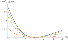
Figure 6: Signal-to-noise ratio of the work for the bosonic swap engine ($\theta=\frac{\pi}{2}$) with $N_{A}=3$ versus occupation number $N_{B}$ for ideal thermalization (solid), and finite thermalization times $\gamma\tau=3.,2.$ and $1.$ (dashed, dotted and dot-dashed, respectively).

The function $h(\beta_{A}\omega_{A}-\beta_{B}\omega_{B})$ in Eq. (25) of the main text is replaced with

$$v(\beta_{A}\omega_{A},\beta_{B}\omega_{B},\gamma\tau)\equiv(\beta_{A}\omega_{A}-\beta_{B}\omega_{B})$$ (86)

$$\times\frac{(1+e^{-\gamma\tau})^{2}\cosh(\beta_{A}\omega_{A})+(1+e^{-\gamma\tau})^{2}\cosh(\beta_{B}\omega_{B})-(1+e^{-2\gamma\tau})\cosh(\beta_{A}\omega_{A}-\beta_{B}\omega_{B})-e^{-\gamma\tau}(4+e^{-\gamma\tau})-1}{(1-e^{-2\gamma\tau})[\sinh(\beta_{A}\omega_{A})-\sinh(\beta_{B}\omega_{B})-\sinh(\beta_{A}\omega_{A}-\beta_{B}\omega_{B})]}\;.$$

One can easily prove the bound

$$v(\beta_{A}\omega_{A},\beta_{B}\omega_{B},\gamma\tau)\geq 2\coth(\gamma\tau/2)\;,$$ (87)

and hence the thermodynamic uncertainty relation

$$\frac{\mbox{var}(W)}{\langle W\rangle^{2}}\geq\frac{2}{\langle\Sigma\rangle}\coth(\gamma\tau/2)+1\;.$$ (88)

This bound shows that thermodynamic uncertainty relations can be informative also for more realistic engines where finite thermalization times are considered. Partial thermalization clearly affects the signal-to-noise ratio of the extracted work. When treating specific microscopic interactions via time-dependent Hamiltonian or assigning a time cost to the unitary transformations, one may study optimal time allocation between thermalization strokes and unitary strokes in order to maximize the extracted work at non-zero power.

The replacement rule $(N_{A},N_{B})\rightarrow(\tilde{N}_{A},\tilde{N}_{B})$ also applies to the joint probability of the stochastic work and heat. This implies that even in the case of partial thermalization the efficiency for the swap engine remains a non-fluctuating quantity. We notice, however, that a detailed fluctuation theorem as in Eq. (12) holds provided that $\beta_{A}$ and $\beta_{B}$ are replaced by the effective inverse temperatures $\tilde{\beta}_{X}=\frac{1}{\omega_{X}}\ln\left(\frac{\tilde{N}_{X}+1}{\tilde{N}_{X}}\right)$.

For arbitrary interaction parameter $\theta$, we argue that the issue of the presence of correlations or coherence in the periodic steady states could be addressed by replacing the two-measurement protocol with a full-counting-statistics approach, along the lines of Ref. soli .

References

• (1) D. Kondepudi and I. Prigogine, Modern Thermodynamics: From Heat Engines to Dissipative Structures (John Wiley & Sons, West Sussex, 2007).
• (2) G. Benenti, G. Casati, K. Saito, and R. S. Whitney, Phys. Rep. 694, 1 (2017).
• (3) N. Li, J. Ren, L. Wang, G. Zhang, P. HΓ€nggi, and B. Li, Rev. Mod. Phys. 84, 1045 (2012).
• (4) F. S. Gnesotto, F. Mura, J. Gladrow, and C. P. Broedersz, Rep. Prog. Phys. 81, 066601 (2018).
• (5) F. Ritort, Nonequilibrium Fluctuations in Small Systems: From Physics to Biology, in Adv. Chem. Phys. 137, 31 (2008).
• (6) R. Rao and M. Esposito, Phys. Rev. X 6, 041064 (2016).
• (7) Y. Dubi and M. Di Ventra, Rev. Mod. Phys. 83, 131 (2011).
• (8) B. Sothmann, R. SΓ‘nchez, and A. N. Jordan, Nanotechnology 26, 032001 (2015).
• (9) D. J. Evans, E. G. D. Cohen, and G. P. Morriss, Phys. Rev. Lett. 71, 2401 (1993).
• (10) G. Gallavotti and E. G. D. Cohen, Phys. Rev. Lett. 74, 2694 (1995).
• (11) C. Jarzynski, Phys. Rev. E 56, 5018 (1997).
• (12) G. E. Crooks, J. Stat. Phys. 90, 1481 (1998).
• (13) B. Piechocinska, Phys. Rev. A 61, 062314 (2000).
• (14) C. Jarzynski, J. Stat. Phys. 98, 77 (2000).
• (15) C. Jarzynski and D. K. WΓ³jcik, Phys. Rev. Lett. 92, 230602 (2004).
• (16) U. Seifert, Phys. Rev. Lett. 95, 040602 (2005).
• (17) U. M. B. Marconi, A. Puglisi, L. Rondoni, and A. Vulpiani, Phys. Rep. 461, 111 (2008).
• (18) K. Saito and Y. Utsumi, Phys. Rev. B 78, 115429 (2008).
• (19) D. Andrieux, P. Gaspard, T. Monnai, and S. Tasaki, New J. Phys. 11, 043014 (2009).
• (20) M. Esposito, U. Harbola, and S. Mukamel, Rev. Mod. Phys. 81, 1665 (2009).
• (21) M. Esposito and C. Van den Broeck, Phys. Rev. Lett. 104, 090601 (2010).
• (22) M. Campisi, P. Talkner, and P. HΓ€nggi, Phys. Rev. Lett. 105, 140601 (2010).
• (23) N. A. Sinitsyn, J. Phys. A 44, 405001 (2011).
• (24) C. Jarzynski, Annu. Rev. Condens. Matter Phys. 2, 329 (2011).
• (25) M. Campisi, P. HΓ€nggi, and P. Talkner, Rev. Mod. Phys. 83, 771 (2011).
• (26) U. Seifert, Rep. Prog. Phys. 75, 126001 (2012).
• (27) M. Campisi, J. Phys. A 47 245001, (2014).
• (28) P. HΓ€nggi and P. Talkner, Nat. Phys. 11, 108 (2015).
• (29) R. Rao and M. Esposito, Entropy 20, 635 (2018).
• (30) A. C. Barato and U. Seifert, Phys. Rev. Lett. 114, 158101 (2015).
• (31) P. Pietzonka, A. C. Barato, and U. Seifert, Phys. Rev. E 93, 052145 (2016).
• (32) T. R. Gingrich, J. M. Horowitz, N. Perunov, and J. L. England, Phys. Rev. Lett. 116, 120601 (2016).
• (33) M. Polettini, A. Lazarescu, and M. Esposito, Phys. Rev. E 94, 052104 (2016).
• (34) P. Pietzonka, F. Ritort, and U. Seifert, Phys. Rev. E 96, 012101 (2017).
• (35) J. M. Horowitz and T. R. Gingrich, Phys. Rev. E 96, 020103(R) (2017).
• (36) K. Proesmans and C. Van den Broeck, Europhys. Lett. 119, 20001 (2017).
• (37) B. K. Agarwalla and D. Segal, Phys. Rev. B 98, 155438 (2018).
• (38) T. Koyuk, U. Seifert, and P. Pietzonka, J. Phys. A 52, 02LT02 (2018).
• (39) A. C. Barato, R. Chetrite, A. Faggionato, and D. Gabrielli, New J. Phys. 20, 103023 (2018).
• (40) K. Brandner, T. Hanazato, and K. Saito, Phys. Rev. Lett. 120, 090601 (2018).
• (41) P. Pietzonka and U. Seifert, Phys. Rev. Lett. 120, 190602 (2018).
• (42) V. Holubec and A. Ryabov, Phys. Rev. Lett. 121, 120601 (2018).
• (43) K. Macieszczak, K. Brandner, and J. P. Garrahan, Phys. Rev. Lett. 121, 130601 (2018).
• (44) J. Li, J. M. Horowitz, T. R. Gingrich, and N. Fakhri, Nat. Commun. 10, 1666 (2019).
• (45) S. Saryal, H. M. Friedman, D. Segal, and B. K. Agarwalla, Phys. Rev. E 100, 042101 (2019).
• (46) A. Dechant, J. Phys. A 52, 035001 (2019).
• (47) K. Proesmans and J. M. Horowitz, J. Stat. Mech. Theor. Exp. 2019, 054005 (2019).
• (48) A. C. Barato, R. Chetrite, A. Faggionato, and D. Gabrielli, J. Stat. Mech. Theor. Exp. 2019, 084017 (2019).
• (49) G. Guarnieri, G. T. Landi, S. R. Clark, and J. Goold, Phys. Rev. Res. 1, 033021 (2019).
• (50) J. M. Horowitz and T. R. Gingrich, Nature Physics 16, 15 (2020).
• (51) N. Merhav and Y. Kafri, J. Stat. Mech. Theor. Exp. 2010, P12022 (2010).
• (52) T. Van Vu and Y. Hasegawa, Phys. Rev. E 100, 012134 (2019).
• (53) P. P. Potts and P. Samuelsson, Phys. Rev. E 100, 052137 (2019).
• (54) A. M. Timpanaro, G. Guarnieri, J. Goold, and G. T. Landi, Phys. Rev. Lett. 123, 090604 (2019).
• (55) Y. Hasegawa and T. Van Vu, Phys. Rev. Lett. 123, 110602 (2019).
• (56) Y. Zhang, arXiv:1910.12862 (2019).
• (57) T. Van Vu and Y. Hasegawa, J. Phys. A 53, 075001 (2020).
• (58) W. De Roeck and C. Maes, Phys. Rev. E 69, 026115 (2004).
• (59) P. Talkner and P. HΓ€nggi, J. Phys. A 40, F569 (2007).
• (60) C. Jarzynski, Phys. Rev. Lett. 78, 2690 (1997).
• (61) T. D. Kieu, Phys. Rev. Lett. 93, 140403 (2004).
• (62) Y. Rezek and R. Kosloff, New J. Phys. 8, 83 (2006).
• (63) H. T. Quan, Y.-x. Liu, C. P. Sun, and F. Nori, Phys. Rev. E 76, 031105 (2007).
• (64) G. Thomas and R. S. Johal, Phys. Rev. E 83, 031135 (2011).
• (65) O. Abah, J. Roßnagel, G. Jacob, S. Deffner, F. Schmidt-Kaler, K. Singer, and E. Lutz, Phys. Rev. Lett. 109, 203006 (2012).
• (66) M. Campisi, J. P. Pekola, and R. Fazio, New J. Phys. 17, 035012 (2015).
• (67) G. De Chiara, G. Landi, A. Hewgill, B. Reid, A. Ferraro, A. J. Roncaglia, and M. Antezza, New J. Phys. 20, 113024 (2018).
• (68) J. P. S. Peterson, T. B. BatalhΓ£o, M. Herrera, A. M. Souza, R. S. Sarthour, I. S. Oliveira, and R. M. Serra, Phys. Rev. Lett. 123, 240601 (2019)
• (69) C. Macchiavello, A. Riccardi, M. F. Sacchi, Phys. Rev. A 101, 062326 (2020).
• (70) L. Mandel and E. Wolf, Optical Coherence and Quantum Optics (Cambridge University Press, Cambridge, 1995)
• (71) G. M. D’Ariano, M. G. A. Paris, and M. F. Sacchi, Nuovo Cimento B 114, 339 (1999).
• (72) E. Lukacs, Characteristic Functions (Griffin, London, 1970).
• (73) N. G. Ushakov, Selected Topics in Characteristics Functions (De Gruyter, Berlin, 2011).
• (74) H. Carmichael, An Open Systems Approach to Quantum Optics, LNP Vol. 18 (Springer, Berin, 1993).
• (75) P. Solinas and S. Gasparinetti, Phys. Rev. E 92, 042150 (2015).