Efficient phonon cascades in hot photoluminescence of WSe₂ monolayers

Abstract

Energy relaxation of photo-excited charge carriers is of significant fundamental interest and crucial for the performance of monolayer (1L) transition metal dichaclogenides (TMDs) in optoelectronics. We measure light scattering and emission in 1L-WSe₂ close to the laser excitation energy (down to $\sim$0.6meV). We detect a series of periodic maxima in the hot photoluminescence intensity, stemming from energy states higher than the A-exciton state, in addition to sharp, non-periodic Raman lines related to the phonon modes. We find a period $\sim$15meV for peaks both below (Stokes) and above (anti-Stokes) the laser excitation energy. We detect 7 maxima from 78K to room temperature in the Stokes signal and 5 in the anti-Stokes, of increasing intensity with temperature. We assign these to phonon cascades, whereby carriers undergo phonon-induced transitions between real states in the free-carrier gap with a probability of radiative recombination at each step. We infer that intermediate states in the conduction band at the $\Lambda$-valley of the Brillouin zone participate in the cascade process of 1L-WSe₂. The observations explain the primary stages of carrier relaxation, not accessible so far in time-resolved experiments. This is important for optoelectronic applications, such as photodetectors and lasers, because these determine the recovery rate and, as a consequence, the devices’ speed and efficiency.

I Introduction

Following optical excitation of a semiconductor above the band gap, the subsequent energy relaxation pathways play an important role in opticsKlimov et al. (1999); Brida et al. (2013); Kozawa et al. (2014) and charge carrier transportSong and Dery (2013); Glazov (2020). These processes are related to hot charge carriers and excitons and are responsible for the determination of the electron mobilityBalkan (1998), optical absorption in indirect band gap semiconductorsPeter and Cardona (2010), and intervalley scattering of hot electronsPeter and Cardona (2010). Photoluminescence (PL) and Raman scattering can be used to probe the interactions of carriers with phonons. In most materials, different types of phonons with different energies can participate in the relaxation process of excited carriers. However, in some materials one type of phonon plays a dominant role and leads to high order processes, e.g., up to 9 longitudinal optical (LO) phonon replicas were reported in the hot PL of CdS and CdSeLeite et al. (1969); Klein and Porto (1969); Gross et al. (1973). Multi-phonon processes are important in defining the optoelectronic performance of ZnOCerqueira et al. (2011); Ursaki et al. (2004); Kumar et al. (2006); Vincent et al. (2008) and GaNSun et al. (2002). Similar effects were measured at 4.2K in bulk MoS₂Gołasa et al. (2014). Reference Brem et al. (2018) predicted that phonon-induced cascade-like relaxation of excitons could be measured in pump-probe experiments of TMDs. Reference Martin and Varma (1971) presented a model whereby electrons (holes), e (h), make successive transitions between real states assisted by the emission of a prominent phonon, while other inelastic scattering processes have negligible probability. This gives rise to multiple Stokes-shifted lines.

Group VI transition metal dichalcogenide monolayers (1L-TMDs) are promising for (opto)electronic devicesFerrari et al. (2015); Koppens et al. (2014) due to their direct band gaps in the visible to near-infraredSplendiani et al. (2010); Mak et al. (2010); Tonndorf et al. (2013a), offering a wide selection of light emission wavelengths at room temperature (RT)Mak et al. (2010); Lien et al. (2019). Their optical properties are dominated by excitons with binding energies of hundreds of meVWang et al. (2018), with spin and valley properties (such as valley-selective circular dichroismCao et al. (2012)) highly beneficial for optoelectronics, valleytronics and spintronicsNovoselov et al. (2016); Mak and Shan (2016); Schaibley et al. (2016); Unuchek et al. (2018); Schneider et al. (2018); Koperski et al. (2017); Dufferwiel et al. (2017); Scuri et al. (2018); Hong et al. (2014); Barbone et al. (2018). In 1L-TMDs charge carriers and excitons interact strongly with phononsSong and Dery (2013); He et al. (2020); Zhang and Niu (2015); Zhu et al. (2018); Trovatello et al. (2019). The optical oscillator strength, i.e. the probability of optical transitions between valence and conduction statesPeter and Cardona (2010), is higher than in III-V quantum wellsPeter and Cardona (2010), resulting in short ($\sim$1psRobert et al. (2016)) exciton lifetimes. This also favors hot PL emission, as excitons relax between several real statesManca et al. (2017); Han et al. (2018).

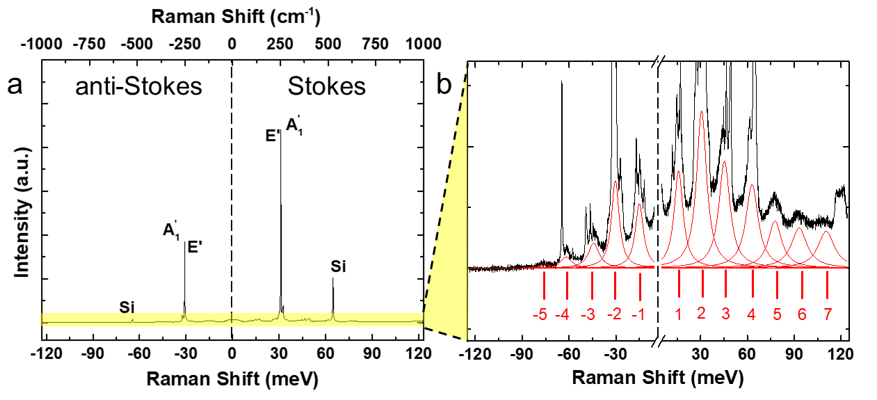
Figure 1: Raman and hot PL spectra of 1L-WSe₂ on SiO₂/Si (a) Emission and scattering spectrum of 1L-WSe₂ at 295K as a function of energy shift with respect to the excitation laser (2.33eV). The degenerate in-plane ($E^{\prime}$) and out-of-plane ($A_{1}^{\prime}$) Raman mode$\sim 250cm^{-1}$Tonndorf et al. (2013b), as well as the Si Raman peak$\sim 521cm^{-1}$Temple and Hathaway (1973), are prominent in both S and AS. (b) Magnified portion of the spectrum in yellow in (a). This reveals 7 periodic S peaks and 5 AS. Their intensity decreases as a function of the energy shift for both S and AS

.

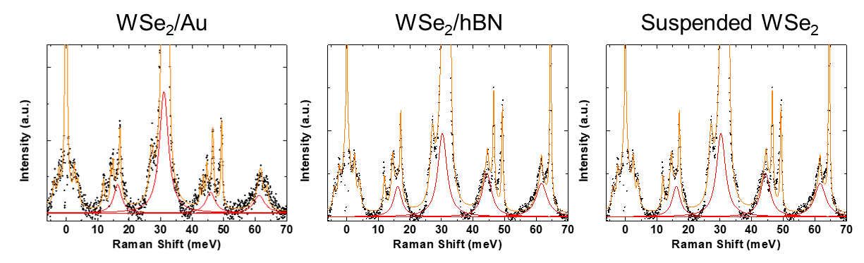
Figure 2: Raman spectra of 1L-WSe₂ on different substrates, at 295K and 514nm. Black points are the experimental data. The red lines are the fitted cascades and yellow line is the sum of the fitted Lorentzians

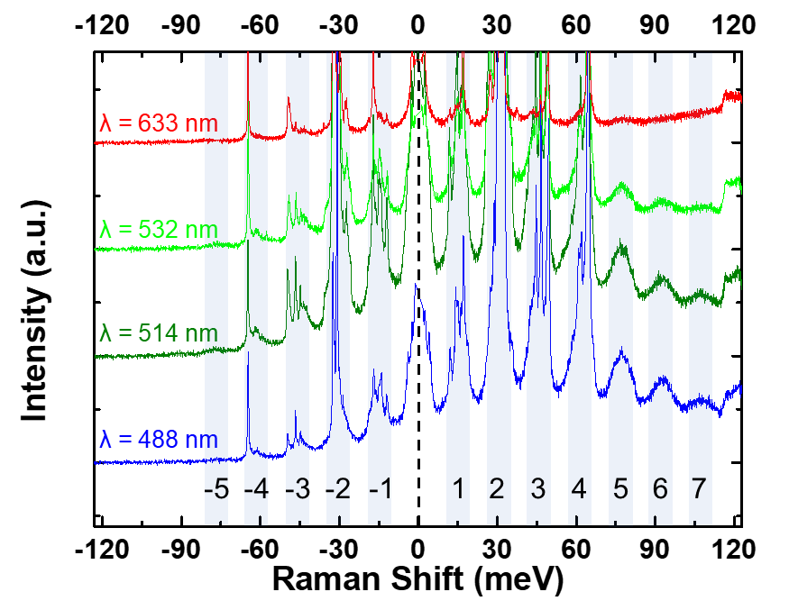
Figure 3: Phonon cascades for different laser energies. Raman spectra of 1L-WSe₂ on SiO₂/Si at 488, 514, 532, 633nm and 295K, shifted vertically for clarity

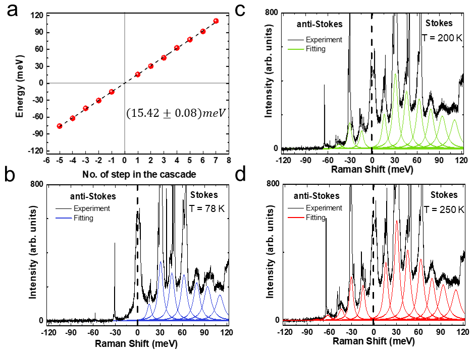
Figure 4: Energy separation and T dependence (a) Emission energies as a function of number of steps in the cascade, extracted from the RT spectrum in Fig.1b. The dashed black line is a linear fit, giving a step energy$\sim$15.42$\pm$0.08meV. (b-d)Hot PL spectra of 1L-WSe₂ at (b) 78K, (c) 200K, (d) 250K for 532nm excitation

Here, we use an ultra-low ($\sim$5cm${}^{-1}\sim$0.6meV) cut-off frequency (ULF) Raman spectroscopy system (Horiba LabRam HR Evolution) to investigate the light scattered and emitted by 1L-WSe₂ on SiO₂, hBN and Au, as well as suspended 1L-WSe₂. We observe phonon-assisted emission of hot PL periodic in energy both in the Stokes (S) and anti-Stokes (AS) spectral range, and we extract a phonon energy $\sim$15meV. The S signal shows 7 maxima at 78$\ldots$295K. We also detect up to 5 maxima in the anti-Stokes signal $\sim$75meV above the laser excitation energy. The AS signal increases in intensity as the temperature (T) is raised. In order to explain the findings, we extend the theory of the cascade model initially developed for bulk crystalsMartin and Varma (1971), to 1L-TMDs. We include finite T effects to compare S and AS signals and to understand carrier relaxation at RT. By analyzing the T and excitation energy dependence of our spectra, we conclude that a continuum of states (in the free-carrier gap) is involved in the e-h relaxation in 1L-WSe₂. Intermediate states in the conduction band around the $\Lambda$-valley of the Brillouin zone (BZ) participate in the cascade process. Hot PL so close in energy to the non-resonant excitation laser gives access to the initial stages of carrier relaxation. These processes are normally ultrafast (e.g. $\sim$100fs in GaAsKash et al. (1985)) and challenging to be traced by time-resolved experiments. Understanding the carrier relaxation pathways in 1L-WSe₂ is important for optoelectronic applications, such as photodetectorsKoppens et al. (2014) and lasersReeves et al. (2018), because it determines the recovery rate (i.e. the population of carriers relaxing to the ground state over time) and, as a result, the devices’ speed and efficiency.

II Results and Discussion

1L-WSe₂ flakes are exfoliated from bulk 2H-WSe₂ crystals (2D Semiconductors) by micromechanical cleavage on Nitto Denko tapeNovoselov et al. (2005), then exfoliated again on a polydimethylsiloxane (PDMS) stamp placed on a glass slide for inspection under optical microscope. Optical contrast is used to identify 1L prior to transferCasiraghi et al. (2007). Before transfer, 85nm (for optimum contrastCasiraghi et al. (2007)) SiO₂/Si substrates are wet cleanedPurdie et al. (2018) (60s ultrasonication in acetone and isopropanol) and subsequently exposed to oxygen-assisted plasma at 10W for 60s. The 1L-WSe₂ flakes are then stamped on the substrate with a micro-manipulator at 40^∘C, before increasing T up to 60^∘C to release 1L-WSe₂Orchin et al. (2019). The same procedure is followed for transfer of 1L-WSe₂ on hBN, Au and Si substrates with 2$\mu$m Au trenches made by lithography, to suspend the samples.

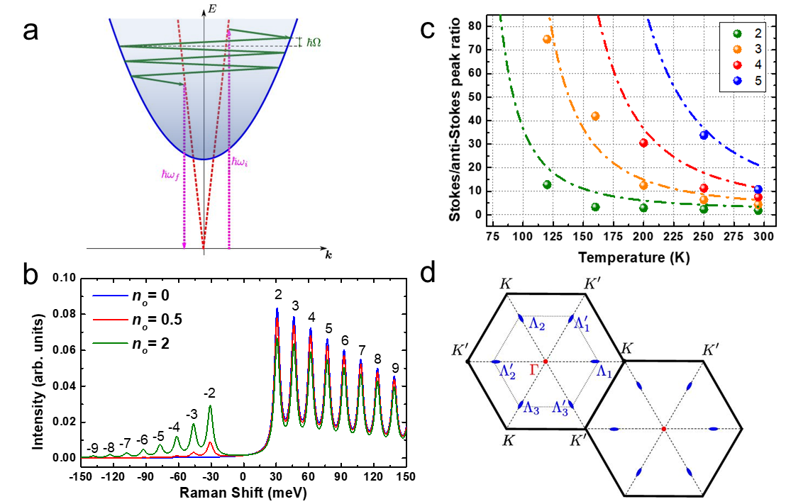
Figure 5: Comparison between experiments and theory (a) Scheme of phonon-assisted hot PL. The incident, $\hbar\omega_{i}$, and outgoing, $\hbar\omega_{f}$, photons are shown by dotted magenta vertical arrows. The phonons participating in the cascade are indicated by the green arrows. The e-h pair dispersion curve is the blue parabola. The light cone is shown by red dashed lines. (b) Calculated S/AS spectrum at different T. (c) I_S/I_AS for different numbers of cascade steps as a function of T. Filled circles are experimental data at 532nm. The fit with Eq.(9) is indicated by dot-dashed lines. (d) Extended BZ of 1L-WSe₂. Corresponding valleys are marked as $\Gamma$, $K$, $K^{\prime}$ and $\Lambda_{i}$, $\Lambda_{i}^{\prime}$ ($i=1,\ldots,3$)

The Raman and hot PL spectra are recorded in a back-reflection geometry with a 50X objective (NA=0.45) and a spot size$\sim 1\mu$m. A liquid nitrogen cryostat (Linkam Scientific) placed on a XY translational stage is used to control $T=78\ldots 295$K and excitation area. Imaging of the sample and monitoring of the excitation spot position are achieved using a set of beam splitters, aligned to a charge-coupled device (CCD) camera. The PL and Raman signals collected in the backward direction are filtered by 3 notch volume Bragg filters with a total optical density (OD)=9. The cut-off frequency is $\sim 5$cm${}^{-1}\sim 0.6$meV. The filtered signals are then focused on the slit of the spectrometer and dispersed by a 1800l/mm grating before being collected by the detector.

A typical RT Raman spectrum for 1L-WSe₂ on SiO₂/Si measured at 532nm is in Fig.1a. The degenerate in-plane, $E^{\prime}$, and out-of-plane, $A_{1}^{\prime}$, modes of 1L-WSe₂Tonndorf et al. (2013b) dominate the spectrum$\sim 250$cm^-1 ($-31$meV) and$\sim 250$cm^-1 ($+31$meV) in the AS and S range. Rescaling the intensity within the region marked in yellow in Fig.1a reveals an underlying periodic pattern, Fig.1b. Hereafter, for the energy scale we use meV instead of cm^-1.

We fit all the peaks between $-120$meV and $+120$meV using Lorentzians (see Methods), as shown in red in Fig.1b. There are 7 S peaks and 5 AS at 295K. The peak$\sim$120meV ($\sim$970cm^-1) originates from a combination of the Si substrate $\Gamma_{1},\Gamma_{12},\Gamma_{25^{\prime}}$ phononsTemple and Hathaway (1973). Although the energy separation between two consecutive peaks is constant, the intensity decreases as a function of energy with respect to the excitation energy (here fixed at 0). To exclude other contributions, such as thin-film interference effectsKlar et al. (2013); Robert et al. (2018), we measure 1L-WSe₂ transferred on Au, suspended, and placed on few-layer (FL) ($\sim$10nm) hBN, Fig.2. The intensity of the hot PL is comparable among the same steps of the cascade and the position of the peaks is the same. Therefore, the cascade is linked to intrinsic relaxation mechanisms of 1L-WSe₂ and not to substrate-induced interference. Henceforth we will focus on 1L-WSe₂ on SiO₂/Si.

To exclude the possibility that our laser is in resonance with a specific transition, we perform variable excitation wavelength experiments at 295K. Figure 3 plots the spectra measured at 488nm ($\sim$2.54eV), 514nm ($\sim$2.41eV), 532nm ($\sim$2.33eV) and 633nm ($\sim$1.96eV). We observe the same high-order features with identical energy separations in both S and AS. All these excitation energies633attention (633) lie above the free carrier gap of 1L-WSe${}_{2}\sim$1.89eVGoryca et al. (2019); Wang et al. (2015); He et al. (2014). Fig.4a plots the energy offset with respect to the excitation laser (here 532nm) of each emission feature as a function of the number of steps in the cascade at 295K. Applying a linear fit, we extract$\sim$15.42$\pm$0.08meV, regardless of substrate and excitation energy. This strong periodic modulation of the detected light intensity suggests that the scattering of photoexcited carriers is dominated by one prominent phonon mode. Since we excite above the free carrier gap of 1L-WSe₂Goryca et al. (2019), the intermediate states of the transitions are real. The e-h pair representation is depicted in Fig.5a.

The lattice T could affect the peaks intensity, as phonon occupation increases with TJellison Jr et al. (1983); Kip and Meier (1990). We thus perform T dependent measurements from 78 to 295K, while keeping the excitation power constant$\sim$26$\mu$W. No emission AS features are observed at 78K, Fig.4b, with the exception of two sharp lines$\sim-30$ and$\sim-60$meV, originating from 1L-WSe₂ and Si Raman modes, respectively. The hot PL peaks are clearly seen at 200K, Fig.4c, and a further increase in intensity is observed at 250K, Fig.4d. Additional measurements at 120, 160, and 295K are performed and used in the fits in Fig.5.

At low T (78K), phonon absorption processes are suppressed because of the insufficient lattice thermal energyJellison Jr et al. (1983). Optical excitation results in free e-h pair formationSteinleitner et al. (2017); Trovatello et al. (2020) or virtual formation of an exciton with small in-plane wavevector ($k\lesssim\omega_{i}/c$ with $\omega_{i}$ the excitation laser frequency). With the subsequent phonon emission, the e-h pair reaches a real final state (blue parabola in Fig.5a), for which radiative recombination is forbidden by momentum conservation. This triggers the cascade relaxation process, whereby at each step a phonon is emitted (or absorbed at elevated T). If the interaction with one phonon mode with energy $\hbar\Omega$ dominates over all other inelastic scattering processes, the exciton loses energy by integer multiples of $\hbar\Omega$Martin and Varma (1971); Peter and Cardona (2010). After emission of several ($\geqslant$2) phonons, the exciton recombines and emits a photon with frequency $\omega_{f}$ in a two-step process via an intermediate state with a small wavevector, for which radiative recombination is momentum allowed. Thus, we have secondary emission or scattering of light with S shift $\omega_{i}-\omega_{f}=j\Omega$, where $j=2,3,\ldots$. $j=\pm 1$ is impossible as we scatter out of the light cone (i.e. light linear dispersion) with the first event. At finite T, in addition to phonon emission, phonon absorption also comes into play and AS emission is observed at $\omega_{f}-\omega_{i}=j\Omega$.

Multiphonon processes that do not involve real states require higher order in the exciton-phonon interactionShree et al. (2018a), and are therefore less probable. In contrast, the process in Fig.3 is resonant, since excitation in the free-carrier gap means all intermediate states are real. This allows us to describe the phonon emission cascade via the kinetic equation for the exciton distribution function $f(\varepsilon)$, where $\varepsilon$ is the exciton energy, as derived in Methods. Since the energy of the exciton changes in each scattering event by $\pm\hbar\Omega$, the distribution function can be written as:

$$f(\varepsilon)=\sum_{j=-\infty}^{\infty}f_{j}\delta(\varepsilon_{0}-j\hbar\Omega)$$ (1)

where $\varepsilon_{0}$ is the excitation energy, $\delta(\varepsilon)$ is the Dirac $\delta$-distribution (the phonon dispersion and phonon damping results in the broadening of the $\delta$-distribution,as detailed in Methods), $f_{j}$ describe the peaks intensity. At the steady state (partial derivative with respect to time equals zero) these obey a set of coupled equations describing the interplay of in- and out-scattering processes:

$$\gamma f_{j}=\gamma_{o}\left[f_{j-1}(n_{o}+1)+f_{j+1}n_{o}\right]+g\delta_{j,0},\\ \quad j=\ldots,-2,-1,0,1,2,\ldots.$$ (2)

where $n_{o}=\left[\exp{\left({\hbar\Omega}/{k_{B}T}\right)}-1\right]^{-1}$ is the phonon mode occupancy at $T$, $\gamma_{o}$ is the rate of the spontaneous phonon emission, $\gamma=\gamma_{o}(2n_{o}+1)+\gamma^{\prime}$, is the total damping rate of the exciton, which includes recombination and inelastic scattering processes $\gamma^{\prime}$. The last term in Eqs.(2), $g\delta_{j,0}$, describes the exciton generation at the energy $\varepsilon_{0}$, and is proportional to the exciton generation rate. Equation (2) has the boundary conditions:

$$\lim_{j\to-\infty}f_{j}=0,\quad f_{K+1}=0,$$ (3)

where $K$ is the maximum number of steps in the cascade:

$$K=\left\lfloor\frac{\hbar\omega_{i}-E_{1}}{\hbar\Omega}\right\rfloor,$$ (4)

with $E_{1}$ the energy of the exciton band bottom. Equations (2) are derived assuming $\gamma_{o}$ and $\gamma^{\prime}$ independent of $\varepsilon$. This assumption is needed to get an analytical solution of Eqs.(2), but can be relaxed, as discussed in Methods.

The general solution of Eqs.(2) is:

$$f_{j}=\begin{cases}Ax_{+}^{j},\quad j<0,\\ Bx_{+}^{j}+Cx_{-}^{j},\quad j\leqslant 0,\\ \end{cases}$$ (5)

where

$$x_{\pm}=\frac{\gamma\pm\sqrt{\gamma^{2}-4n_{o}(n_{o}+1)\gamma_{o}^{2}}}{2\gamma_{o}n_{o}},$$ (6)

and $x_{+}>1$ and $x_{-}<1$, $A$, $B$, and $C$ are the coefficients. For cascades with $K\gg 1$ we can set $B=0$ and

$$A=C=\frac{g}{\sqrt{\gamma^{2}-4n_{o}(1+n_{o})\gamma_{o}^{2}}}\\ =\frac{g}{\sqrt{\gamma_{o}^{2}+\gamma^{\prime 2}+2\gamma_{o}\gamma^{\prime}(1+2n_{o})}}.$$ (7)

In this model, the spectrum of the scattered light consists of peaks with I$\propto f_{j}$, with scattering cross-section:

$$\sigma(\omega_{i},\omega_{f})=\sigma_{0}(\omega_{i},\omega_{f})\\ \times\left.\sum_{j=2}^{\infty}\right.^{\prime}\frac{1}{\pi}\frac{2\Gamma}{4\Gamma^{2}+(j\Omega-\omega_{i}+\omega_{f})^{2}}f_{j}.$$ (8)

Here $\sigma_{0}(\omega_{i},\omega_{f})$ is a smooth function of frequency, $\Gamma$ is the phonon damping. This description is valid for peaks with $|j|>1$, the prime at the summation denotes that the terms with $j=0,\pm 1$ are excluded. Accordingly, the peaks with Raman shift $\pm\hbar\Omega$ are suppressed. At $n_{o}\to 0$ (limit of low T), $x_{+}\gg 1$ and $\mathrm{I}_{j}$ with negative $j$ (AS components) are negligible. At the same time, $x_{-}\to(\gamma_{o}/\gamma)$ and the S peak intensities, I_S, scale as $(\gamma_{o}/\gamma)^{j}$. This scaling is natural for cascade processesPeter and Cardona (2010); Ivchenko et al. (1977a); Goltsev et al. (1983), since the probability of phonon emission relative to all other inelastic processes is given by $\gamma_{o}/\gamma$, thus I_S decays in geometric progression. At finite T, the AS peaks appear with I_AS proportional to the thermal occupation of the phonon modes. Thus I_S/I_AS with $j$ steps in the cascade can be written as:

$$\frac{\mathrm{I}_{S}(j)}{\mathrm{I}_{AS}(j)}=\frac{f_{j}}{f_{-j}}=\left(1+\frac{1}{n_{o}}\right)^{j},$$ (9)

and corresponds to the ratio of phonon emission and absorption rate to the power of $j$.

The calculated I distribution and spectra at various T (corresponding to different $n_{o}$) are in Fig.5b. Fig.5c plots I_S/I_AS as a function of T from Eq.(9). The experimental points collected from the fitted I of each step in the cascade at 532nm excitation are displayed with circles. The absence of data at 78K indicates no detection of I_AS at this T. Applying Eq.(9) to the steps 2 to 5 in the cascade with a phonon energy$\sim$15.4meV extracted from Fig.4a, gives the dashed lines in Fig.5c, in good agreement with experiments.

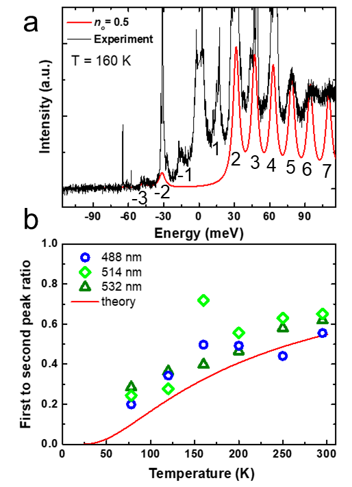
Figure 6: (a) Experimental data at 160K (black line) compared to the calculated spectrum from Eq.(2) for $n_{o}$=0.5. (b) Ratio of measured intensities of $j=1$ to $j=2$ peaks and corresponding fit with Eq.(28)

Our model well captures the main experimental observations. The periodic pattern of hot PL I is reproduced by the calculations, Fig.5b, and I_S/I_AS closely follows Eq.(9), Fig.5c. There is good agreement between our experimental data and the calculated spectra from Eq.(2). An example for $n_{o}$=0.5 at 160K is in Fig.6a. In our model, the peaks with $j=\pm 1$ are absent because $N\geqslant 2$ phonons are needed for the first step of the cascade process, as for Fig.5a. Fig.1 shows that $j=\pm 1$ peaks are smaller than $j=\pm 2$ ones, but still detectable. One scenario disregarded in our model is a process where the two phonons are emitted and then one is absorbed (or vice versa). In this case $\mathrm{I}_{j=1}/\mathrm{I}_{j=2}$ should be strongly T dependent in the $78\ldots 295$K range. This is indeed the case in our experiment, Fig.6b. This additional channel is also based on the interaction with the same phonon energy$\sim$15meV. Another possible effect is elastic scattering of excitons by disorder or acoustic phonons, whereby exciton transitions in and out of the light cone can be controlled by elastic scattering (see Methods for details).

To get a better understanding of the relaxation pathways, we consider different scattering mechanisms.

Scattering within the same valley is not plausible due to the mismatch of BZ centre phonon energiesHe et al. (2020). $\sim$15meV could correspond to either $\Gamma-K$ or $\Gamma-\Lambda$ phonons. The phonon dispersion in 1L-WSe₂ show acoustic phonons with energies$\sim$15meVHe et al. (2020); Jin et al. (2014). These have a flat dispersion, necessary to observe the high number of oscillations we report, and are compatible with the model in Fig.5a.

Another option involves $K$-$K^{\prime}$ scattering of e (h) or, equivalently, $\Gamma$-$K$ scattering of excitons. This would result in I oscillations as a function of the step in the cascade, due to the suppression of the process $\Gamma\rightarrow K\rightarrow K^{\prime}\rightarrow\Gamma$ compared to $\Gamma\rightarrow K\rightarrow\Gamma$ (see Methods for details). However, we do not observe I oscillations for different cascade steps in our spectra. As a result, we exclude this scenario. Therefore, the excitonic states in the $\Lambda$ valleys play a role as intermediate states, Fig.5d. The conduction band minima in these valleys are relatively close ($\sim$35meV) to $K$ and play a crucial role in exciton formation and relaxationKormanyos et al. (2015); Selig et al. (2018); Madéo et al. (2020); Lindlau et al. (2017); Rosati et al. (2020). In this case, h remain in $K$ (or $K^{\prime}$), but e scatter to any of the 6 available $\Lambda$ valleys and then scatter between these $\Lambda$ valleys before going back to $K$ ($K^{\prime}$). This can be described taking into account all pathways, as:

$$\mbox{photon}\to\Gamma\xrightarrow{\hbar\Omega}\underbrace{\Lambda_{i}\xrightarrow{\hbar\Omega}\ldots\xrightarrow{\hbar\Omega}\Lambda_{j}^{\prime}}_{j}\xrightarrow{\hbar\Omega}\mbox{photon},$$

with arbitrary number of steps $j$ (both odd and even). The matrix elements of the processes are similar.

Similar oscillations can appear for free e and hMartin and Varma (1971). The basic description of the effect is similar to what we observe here, and our model can be extended to take into account the e/h distribution functions. The spectra of scattered light and I_S/I_AS are similar to those calculated above. We cannot distinguish between exciton and the free carrier cascades directly in our experiments. The excitonic description, however, seems straightforward due to enhanced (with respect to bulk materials) Coulomb effects in 1L-TMDsWang et al. (2018).

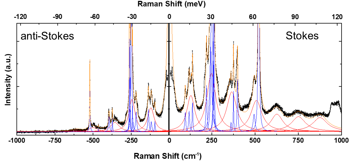
Figure 7: Fitted 1L-WSe₂/SiO₂/Si spectrum, collected at 295K and 532nm

III Conclusions

We investigated the light scattered and emitted 1L-WSe₂ excited above the free carrier gap. We detected a periodic modulation of phonon-assisted hot PL with a period$\sim$15meV both in Stokes and anti-Stokes. We measured the evolution I_S and I_AS for the periodic steps from 78 to 295K. We explained these high-order processes using a cascade model where electrons (holes) make successive transitions between real states with a finite probability of radiative recombination at each step. The electron states in the $\Lambda$ valleys play a role as intermediate states for efficient exciton relaxation. Our findings provide fundamental understanding of the initial steps of exciton relaxation dynamics in 1L-WSe₂ and are valuable for tailoring optoelectronic applications based on this material.

IV Acknowledgements

We acknowledges funding from ANR 2D-vdW-Spin, ANR MagicValley, the Institut Universitaire de France, the RFBR and CNRS joint project 20-52-16303, EU Graphene Flagship, ERC Grants Hetero2D and GSYNCOR, EPSRC Grants EP/K01711X/1, EP/ K017144/1, EP/N010345/1, EP/L016087/1.

V Methods

V.1 Raman and PL spectra fitting

Fig.7 shows representative data fits. The spectrum, measured at 295K at 532nm, is shown with black dots. Lorentzians are used to fit the Raman peaks (FWHM$\sim$1-10cm^-1) and are shown in blue. The residual spectral weight is also fitted with Lorentzians and results into the broader (FWHM$\sim$50-80cm^-1) peaks of the hot PL, shown in red.

V.2 Diagrammatic calculation of Stokes scattering at 0K

For 0K, we calculate the S emission. The light scattering cross-section can be written as (disregarding polarization dependence):

$$\sigma(\omega_{i},\omega_{f})=s\sum_{k}S_{k}(\omega_{i},\omega_{f}),$$ (10)

where $s$ is a prefactor weakly dependent on the initial and final frequencies, $S_{k}(\omega_{i},\omega_{f})$ is the effective cross-section due to the participation of $k$ phonons in the intermediate states, shown by green arrows in Fig.5a. We assume that photoexcitation results in the generation of excitons due to their high (hundreds of meV) binding energiesWang et al. (2018). The description in the case of unbound e-h pairs is similar and outlined below.

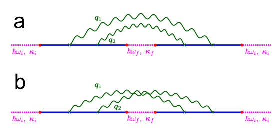
Figure 8: (a-b) Feynman diagrams corresponding to the two-phonon processes. The dotted magenta lines are the photon Green functions in the free space. Blue lines are exciton Green functions (retarded ones at the left-hand side, before the internal photon function, and advanced at the right-hand side). Wiggly lines are phonon Green functions $D^{-}$.

The calculation of the partial contributions $S_{k}(\omega_{i},\omega_{f})$ can be performed in the framework of the diagram technique of Refs.Zeyher (1975); Ivchenko et al. (1977a); Goltsev et al. (1983). We extend their treatment to the two-dimensional case, with the exciton-phonon interaction described by the matrix element $M_{0}$, independent of wavevector. Phonons, as in Refs.He et al. (2020); Jin et al. (2014), are considered as dispersionless. This is reasonable for 1L-TMDs where Fröhlich coupling is suppressedDanovich et al. (2016); Glazov et al. (2019). Following Ref.Glazov et al. (2019), we introduce the coupling constant:

$$\beta=\frac{2\mathcal{S}m|M_{0}|^{2}}{\hbar^{3}\Omega},$$ (11)

where $\mathcal{S}$ is the normalization area, $m$ the exciton translational mass and $\Omega$ the phonon frequency. We focus on one excitonic band (stemming from $1s$ excitons), and disregard the multivalley structure of 1L-TMDsWang et al. (2018) for simplicity. The exciton damping rate in the state with wavevector $\bm{k}$ due to emission of dispersionless phonons is given by:

$$\begin{split}\gamma_{o,k}=\frac{1}{2\tau_{o,k}}=\frac{\pi}{\hbar}\sum_{\bm{k}^{\prime}}|M_{0}|^{2}\delta(E_{k}-E_{k^{\prime}}-\hbar\Omega)=\\ \frac{\beta\Omega}{4}\Theta(E_{k}-\hbar\Omega),\end{split}$$ (12)

where $E_{k}=\hbar^{2}k^{2}/2m$ is the exciton dispersion, $\Theta(x)$ is the Heaviside step function. The total damping rate of the exciton $\gamma_{k}>\gamma_{o,k}$ contains also the contributions due the interaction with acoustic phononsChristiansen et al. (2017); Shree et al. (2018b), disorderMartin et al. (2018), non-radiativeMartin et al. (2018) and radiative (for states within the light cone) dampingSchneider et al. (2018).

Correspondingly, the exciton retarded Green functions read:

$$G(\varepsilon,\bm{k})=\frac{1}{\varepsilon-E_{k}+\mathrm{i}\gamma_{k}}.$$ (13)

By labelling $\Gamma_{q}$ the phonon damping, the Green functions become:

$$D(\omega,\bm{q})=\frac{1}{\hbar\omega-\hbar\Omega+\mathrm{i}\Gamma_{q}},$$ (14)

$$D^{-}(\omega,\bm{q})=D(\omega,\bm{q})-D^{*}(\omega,\bm{q})=\frac{-2\mathrm{i}\Gamma_{q}}{(\hbar\omega-\hbar\Omega)^{2}+\Gamma_{q}^{2}}.$$

Figure 8a illustrates the relevant diagrams describing the two-phonon process:

$$S_{2}^{(a)}=-|M_{0}|^{4}\sum_{\bm{k}}\int_{-\infty}^{\infty}\frac{d\omega}{2\pi}G(\hbar\omega_{i}-E_{1},\bm{\kappa}_{i})\\ \times G(\hbar\omega_{i}-E_{1}-\hbar\omega,\bm{k})G(\hbar\omega_{f}-E_{1},\bm{\kappa}_{f})\\ \times D^{-}(\omega,\bm{\kappa}_{i}-\bm{k})D^{-}(\omega_{i}-\omega_{f}-\omega,\bm{k}-\bm{\kappa}_{f})\\ \times G^{*}(\hbar\omega_{i}-E_{1},\bm{\kappa}_{i})G^{*}(\hbar\omega_{i}-E_{1}-\hbar\omega,\bm{k})G^{*}(\hbar\omega_{f}-E_{1},\bm{\kappa}_{f})\\ =-|M_{0}|^{4}\left|G(\hbar\omega_{i}-E_{1},\bm{\kappa}_{i})\right|^{2}\left|G(\hbar\omega_{f}-E_{1},\bm{\kappa}_{f})\right|^{2}\\ \times\sum_{\bm{k}}\int_{-\infty}^{\infty}\frac{d\omega}{2\pi}D^{-}(\omega,\bm{\kappa}_{i}-\bm{k})D^{-}(\omega_{i}-\omega_{f}-\omega,\bm{k}-\bm{\kappa}_{f})\\ \times\left|G(\hbar\omega_{i}-E_{1}-\hbar\omega,\bm{k})\right|^{2}.$$ (15a)

$$S_{2}^{(b)}=-|M_{0}|^{4}\left|G(\hbar\omega_{i}-E_{1},\bm{\kappa}_{i})\right|^{2}\left|G(\hbar\omega_{f}-E_{1},\bm{\kappa}_{f})\right|^{2}\\ \times\sum_{\bm{k}}\int_{-\infty}^{\infty}\frac{d\omega}{2\pi}D^{-}(\omega,\bm{\kappa}_{i}-\bm{k})D^{-}(\omega_{i}-\omega_{f}-\omega,\bm{k}-\bm{\kappa}_{f})\\ \times G(\hbar\omega_{i}-E_{1}-\hbar\omega,\bm{k})G^{*}(\hbar\omega_{f}-E_{1}+\hbar\omega,\bm{\kappa}_{i}+\bm{\kappa}_{f}-\bm{k})$$ (15b)

where $E_{1}=E_{g}-E_{b,1s}$ is the $1s$ exciton excitation energy, $E_{b,1s}$ is its binding energy.

Figure 8a describes the process where two phonons are emitted one after another. Figure 8b shows the quantum interference of two-photon emission processesIvchenko et al. (1977a). When $\Gamma_{q}\gg\gamma_{k}$, the contribution in Fig.8b and given by Eq.(15b), is smaller by a factor $\gamma_{k}/\Gamma_{q}$, compared to the non-crossing contribution in Fig.8a.

We now focus on the more realistic case where $\Gamma_{q}\ll\gamma_{k}$. For simplicity we disregard the $k$-dependence of $\gamma_{k}$ and the $q$-dependence of $\Gamma_{q}$ and omit the corresponding subscripts. Thus:

$$S_{2}^{(a)}=\frac{4\Gamma}{4\Gamma^{2}+(2\Omega-\omega_{i}+\omega_{f})^{2}}|M_{0}|^{2}\left|G(\hbar\omega_{i}-E_{1},\bm{\kappa}_{i})\right|^{2}\\ \times\left|G(\hbar\omega_{f}-E_{1},\bm{\kappa}_{f})\right|^{2}\\ \times\frac{1}{\hbar}\sum_{\bm{k}}\frac{|M_{0}|^{2}}{\hbar^{2}\gamma^{2}+(\hbar\Omega+\hbar\omega_{f}-E_{1}-E_{k})^{2}}$$ (16a)

$$S_{2}^{(a)}=\frac{4\Gamma}{4\Gamma^{2}+(2\Omega-\omega_{i}+\omega_{f})^{2}}|M_{0}|^{2}\\ \times\left|G(\hbar\omega_{i}-E_{1},\bm{\kappa}_{i})\right|^{2}\left|G(\hbar\omega_{f}-E_{1},\bm{\kappa}_{f})\right|^{2}\frac{1}{\hbar}\\ \times\sum_{\bm{k}}\frac{|M_{0}|^{2}}{(\hbar\omega_{f}+\hbar\Omega-E_{1}-E_{k}+\mathrm{i}\gamma)}\\ \times\frac{1}{(\hbar\omega_{f}+\hbar\Omega-E_{1}-E_{k^{\prime}}-\mathrm{i}\gamma)},$$ (16b)

with $\bm{k}^{\prime}=\bm{\kappa}_{i}+\bm{\kappa}_{f}-\bm{k}$.

Note that

$$\frac{1}{\hbar}\sum_{\bm{k}}\frac{|M_{0}|^{2}}{\hbar^{2}\gamma^{2}+(\hbar\Omega+\hbar\omega_{f}-E_{1}-E_{k})^{2}}=\frac{\gamma_{o}}{\gamma},\\ \frac{1}{\hbar}\sum_{\bm{k}}\frac{|M_{0}|^{2}}{(\hbar\omega_{f}+\hbar\Omega-E_{1}-E_{k}+\mathrm{i}\gamma)}\\ \times\frac{1}{(\hbar\omega_{f}+\hbar\Omega-E_{1}-E_{k^{\prime}}-\mathrm{i}\gamma)}=\\ \frac{\gamma_{o}/\gamma}{\sqrt{1+\left(\frac{|\bm{\kappa}_{i}+\bm{\kappa}_{f}|v}{2\gamma}\right)^{2}}},$$ (17a)

where $v=\sqrt{2(\hbar\omega_{f}+\hbar\Omega-E_{1})/m}$. Thus:

$$\begin{split}S_{2}^{(a)}=\frac{4\Gamma}{4\Gamma^{2}+(2\Omega-\omega_{i}+\omega_{f})^{2}}|M_{0}|^{2}\\ \times\frac{\gamma_{o}}{\gamma}\left|G(\hbar\omega_{i}-E_{1},\bm{\kappa}_{i})\right|^{2}\left|G(\hbar\omega_{f}-E_{1},\bm{\kappa}_{f})\right|^{2},\end{split}$$ (18a)

$$S_{2}^{(b)}=\frac{S_{2}^{(a)}}{\sqrt{1+\left(\frac{|\bm{\kappa}_{i}+\bm{\kappa}_{f}|v}{2\gamma}\right)^{2}}}.$$ (18b)

The factor

$$\frac{|\bm{\kappa}_{i}+\bm{\kappa}_{f}|v}{2\gamma}\sim\frac{l_{\rm eff}}{\lambda},$$

where $l_{\rm eff}$ is the effective mean free path of the exciton, and $\lambda$ is the characteristic wavelength of light. In backscattering in plane, since scattered light is emitted by both 1L-WSe₂ sides:

$$\bm{\kappa}_{f}=-\bm{\kappa}_{i},$$ (19)

the diagram with crossed phonon lines doubles the result stemming from the diagram in Fig.8b. This is due to coherent backscattering (or weak localization) effectIvchenko et al. (1977b); Glazov (2020). Otherwise the contribution of the diagram Fig.8b is negligible, provided that $l_{\rm eff}\gg\lambda$. While the latter condition may not be strictly fulfilled in 1L-TMDsGlazov (2020), we disregard the contributions due to the crossed diagrams to provide an analytical model.

Importantly, the phonon scattering is resonant, taking place via real intermediate states and, accordingly, the scattering cross-section acquires a factor $\frac{\gamma_{o}}{\gamma}$, which gives the probability for an exciton to emit a phonon during its lifetime in a state with wavevector $\bm{k}$. If inelastic scattering is dominated by a single phonon mode, $\gamma_{o}/\gamma$ can be close to unity.

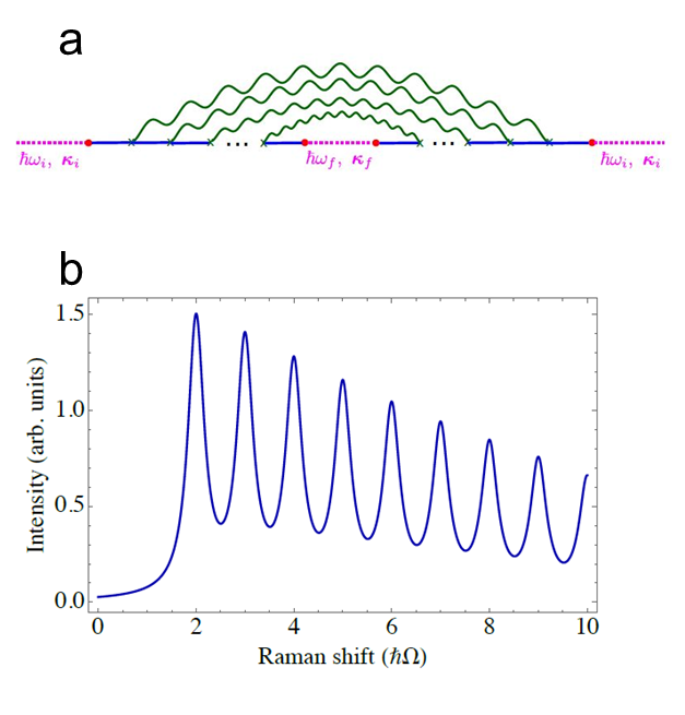
Figure 9: (a) Multiphonon scattering in the non-crossing approximation. (b) Hot PL for $\gamma_{o}/\gamma=0.9$, $\Gamma/\Omega=0.1$, $K=10$.

We now consider multiphonon processes. Within the non-crossing approximation, where we take into account the diagrams where the phonon propagators do not cross, i.e., we disregard the interference of the phonons, we can sum the contributions of the diagrams in Fig.9a with $k=2,3,\ldots$ phonon lines.

The maximum number of phonons involved in the process is given by Eq. (4). Performing the calculations analogous to those presented above we get Eq. (8). In particular for $K\to\infty$ we get:

$$\begin{split}\sigma(\omega_{i},\omega_{f})=\sigma_{0}(\omega_{i},\omega_{f})\frac{x}{\pi}\\ \times\Re\left\{\frac{{}_{2}F_{1}\left(1,\frac{-2\mathrm{i}\Gamma+2\Omega-\omega_{i}+\omega_{f}}{\Omega},\frac{-2\mathrm{i}\Gamma+3\Omega-\omega_{i}+\omega_{f}}{\Omega},x\right)}{2\Gamma+\mathrm{i}(2\Omega-\omega_{i}+\omega_{f})}\right\},\end{split}$$ (20)

with ${}_{2}F_{1}(a,b,c,x)$ the hypergeometric function, and $x=\gamma_{o}/\gamma$.

A typical calculated spectrum at 0K considering the S component of the emission is in Fig.9b. Each cascade step provides a factor $\gamma_{o}/\gamma$ to the scattering cross-section. If the scattering rates $\gamma_{o}$ and $\gamma$ are energy dependent, the S component of emission at $j$th step is given by the products

$$\mathrm{I}_{j}\propto\prod_{k=2}^{j}\frac{\gamma_{o}(k)}{\gamma(k)},$$ (21)

where the argument $k$ denotes the step of the cascade (i.e., the energy) where the corresponding scattering rate is taken.

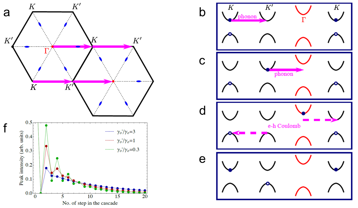
Figure 10: Schematic band diagram and scattering pathways in e-h representation. (a) Extended BZ with $K$ valley shown twice for convenience. (b) Initial state $\Gamma$ ($K-K$) exciton. (c) After first phonon scattering $K$ ($K^{\prime}-K$) exciton. (d) After second phonon scattering we have $K^{\prime}$-like ($\Gamma-K$) exciton. (e) e-h interaction brings a $\Gamma-K$ exciton to the $K^{\prime}$-exciton ($K-K^{\prime}$). Open circle denotes empty state (h state can be obtained by time-reversal). (f) Scattered I accounting for $\Gamma\to K\to K^{\prime}$ photon-assisted transitions for $\gamma^{\prime}/\gamma_{o}=0.3$, $\gamma^{\prime\prime}/\gamma_{o}=0.3$, at 0K

In the presence of static disorder, or quasi-elastic acoustic phonon scattering with negligible energy transfer, additional diagrams with the corresponding scattering processes should be taken into account. To illustrate that elastic scattering processes do not suppress oscillations in the Raman and hot PL, we consider exciton scattering by static impurities with scattering rate $\gamma_{\rm imp}$, with $\gamma$, the total exciton scattering rate. Taking into account diagrams similar to Fig.9a, but with impurity lines, $\gamma_{o}/\gamma$ is renormalized by elastic scattering as:

$$\frac{\gamma_{o}}{\gamma}\to\frac{\gamma_{o}}{\gamma}\sum_{n=0}^{\infty}\left(\frac{\gamma_{\rm imp}}{\gamma}\right)^{n}=\frac{\gamma_{o}}{\gamma-\gamma_{\rm imp}}.$$ (22)

This means that for elastic scattering the exciton energy does not change, thus it does not smear-out the I oscillations.

V.3 Kinetic equation

The non-crossing approximation corresponds to a kinetic equation model where the exciton dynamics after optical excitation is described by the Boltzmann equation in the formTserkovnikov (1993):

$$\gamma^{\prime}f(\bm{k})=\sum_{\bm{k}^{\prime}}W_{\bm{k}\bm{k}^{\prime}}[f_{\bm{k}^{\prime}}-W_{\bm{k}^{\prime}\bm{k}}f_{\bm{k}}]+g_{\bm{k}}.$$ (23)

with $W_{\bm{k}^{\prime}\bm{k}}$ the transition rate between states with wavevectors $\bm{k}$ and $\bm{k}^{\prime}$, with phonon emission or absorption. For simplicity, we disregard elastic scattering. $\gamma^{\prime}$ is the damping rate unrelated to exciton-phonon interaction, $g_{\bm{k}}$ is the exciton generation rate. The kinetic equation also allows us to account for finite T effectsTserkovnikov (1993).

It is convenient to average $f_{\bm{k}}$ over the in-plane directions of $\bm{k}$, and consider just the exciton energy distribution function $f(\varepsilon)$. The latter can be recast as [cf. Eq. (1)]:

$$f(\varepsilon)=\sum_{j=-\infty}^{\infty}f_{j}\delta(\varepsilon_{0}-j\hbar\Omega),$$ (24)

with $f_{j}$ satisfying the set of equations:

$$\begin{split}\gamma f_{j}=\gamma_{o}\left[f_{j-1}(n_{o}+1)+f_{j+1}n_{o}\right]+g_{j},\\ \quad j=\ldots,-2,-1,0,1,2,\ldots,\end{split}$$ (25)

where

$$n_{o}=\frac{1}{\exp{\left(\frac{\hbar\Omega}{k_{B}T}\right)}-1},$$

is the phonon mode occupancy at T, $\gamma_{o}$ is the rate of spontaneous phonon emission,

$$\gamma=\gamma_{o}(2n_{o}+1)+\gamma^{\prime},$$

is the total exciton damping rate. $g_{j}$ is the exciton generation rate in the state $j$ related to the process of virtual formation of the exciton within the light cone, and its consequent relaxation to the real state with the phonon emission or absorption. Thus, the non-zero values of $g_{j}$ are:

$$g_{1}=g(n_{o}+1),\quad g_{-1}=gn_{o},$$ (26)

with $g$ a parameter. In the main text we replaced the generation rate Eq.(26) with a simplified model with $g_{0}=g\neq 0$. This is also valid if elastic scattering is strong and excitons can leave the light cone via static defect scattering.

Since photon emission requires a phonon-induced transition, I of peak $j$ with phonon-induced energy shift $j\hbar\Omega$ is given by:

$$I_{j}=f_{j-1}\gamma_{o}(n_{o}+1)+f_{j+1}\gamma_{o}n_{o}\propto f_{j}.$$ (27)

The last proportionality is due to the kinetic Eq.(25) and is valid for $j\neq 0,\pm 1$.

We now address I of $|j|=1$ peaks. We consider $I_{j=1}/I_{j=2}$ as plotted in Fig.6. The mechanisms of $j=1$ peak formation are as follows. (i) Elastic disorder-induced scattering, Eq.(22), which provides a transfer between states within the light cone and states at the dispersion. (ii) Combination of phonon emission and absorption, where the $j=1$ peak appears as a result of two phonon emission followed by one phonon absorption. In (i) $I_{j=1}/I_{j=2}$ is not dependent on T, while in (ii):

$$\frac{I_{j=1}}{I_{j=2}}=\exp{\left(-\frac{\hbar\Omega}{k_{B}T}\right)},$$ (28)

strongly depends on T. The results of Eq.(28) and plotted in Fig.6 by a solid line and agree with experiments. Elastic processes could be the origin of a small offset between the experiment and the fitted curve.

V.4 Cascades in a free carriers model

Cascades in phonon-assisted hot PL are possible for free carriers, i.e., for e-h pairs in the continuum states. In this situation the phonon-assisted e/h relaxation is independent, and governed by Eq.(25). Light scattering can be represented as

$$\mbox{photon}\to\mbox{electron,}\bm{k}+\mbox{hole,}\bm{k}$$

$$\xrightarrow{\hbar\Omega}\mbox{electron,}\bm{k}-\bm{q}+\mbox{hole,}\bm{k}\ldots$$

$$\xrightarrow{\hbar\Omega}\mbox{electron,}\bm{k}+\mbox{hole,}\bm{k}\to\mbox{photon}.$$

Accordingly, we expect oscillations in scattered light I with period $\hbar\Omega$.

V.5 Intervalley scattering model

We now consider the case of exciton scattering enabled by BZ edge phonons with wavevectors $\bm{Q}\sim\pm\bm{K}$. An exciton scatters between the $\Gamma$ valley ($K-K$ or $K^{\prime}-K^{\prime}$ exciton) and $K/K^{\prime}$ valleys ($K^{\prime}-K$ and $K-K^{\prime}$ excitons), Fig.10a. Photon emission occurs only for the states with small wavevectors ($\sim$the photon ones), according to the paths:

$$\mbox{photon}\to\Gamma\xrightarrow{\hbar\Omega}K\xrightarrow{\hbar\Omega}\mbox{photon};$$

$$\mbox{photon}\to\Gamma\xrightarrow{\hbar\Omega}K\xrightarrow{\hbar\Omega}K^{\prime}\xrightarrow{\hbar\Omega}\mbox{photon};$$

$$\mbox{photon}\to\Gamma\xrightarrow{\hbar\Omega}K\xrightarrow{\hbar\Omega}\Gamma\xrightarrow{\hbar\Omega}K\xrightarrow{\hbar\Omega}\mbox{photon};$$

$$\mbox{photon}\to\Gamma\xrightarrow{\hbar\Omega}K\xrightarrow{\hbar\Omega}\Gamma\xrightarrow{\hbar\Omega}K^{\prime}\xrightarrow{\hbar\Omega}\mbox{photon};\ldots$$

Processes like “$\Gamma\xrightarrow{\hbar\Omega}\mbox{photon}$” are forbidden due to momentum conservation.

The set of equations describing the processes is:

$$\gamma_{\Gamma}f_{j}^{\Gamma}=\gamma_{o}\left[f_{j-1}^{K}(n_{o}+1)+f_{j+1}^{K}n_{o}\right]+\\ \gamma_{o}\left[f_{j-1}^{K^{\prime}}(n_{o}+1)+f_{j+1}^{K^{\prime}}n_{o}\right]+g\delta_{j,0},\\ \gamma_{K}f_{j}^{K}=\gamma_{o}\left[f_{j-1}^{\Gamma}(n_{o}+1)+f_{j+1}^{\Gamma}n_{o}\right]+\\ \gamma_{o}^{\prime}\left[f_{j-1}^{K^{\prime}}(n_{o}+1)+f_{j+1}^{K^{\prime}}n_{o}\right],\\ \gamma_{K^{\prime}}f_{j}^{K^{\prime}}=\gamma_{o}\left[f_{j-1}^{\Gamma}(n_{o}+1)+f_{j+1}^{\Gamma}n_{o}\right]+\\ \gamma_{o}^{\prime}\left[f_{j-1}^{K}(n_{o}+1)+f_{j+1}^{K}n_{o}\right].$$ (29a)

with $f_{j}^{\Gamma}$, $f_{j}^{K}$ and $f_{j}^{K^{\prime}}$ the exciton occupancies in the corresponding valley. $\gamma_{o}$ and $\gamma_{o}^{\prime}$ are the photon spontaneous emission rates for the scattering processes $\Gamma\leftrightarrow K/K^{\prime}$ and $K\leftrightarrow K^{\prime}$, respectively, and the decay rates

$$\gamma_{\Gamma}=\gamma_{o}(2n_{o}+1)+\gamma^{\prime},\quad\gamma_{K}=\gamma_{K^{\prime}}=(\gamma_{o}+\gamma_{o}^{\prime})(2n_{o}+1)+\gamma^{\prime\prime}.$$

The scattering processes in the e-h picture are presented in Figs.10b-e. These demonstrate that $\gamma_{o}$ and $\gamma_{o}^{\prime}$ are different because the second process ($K\leftrightarrow K^{\prime}$) needs additional Coulomb interaction, Figs.10c-e. Thus, direct phonon-induced $K\leftrightarrow K^{\prime}$ transfer is impossible, and the corresponding process takes place via an intermediate state with e in the $\Gamma$ valley. The results of the calculations in Fig.10f demonstrate that pronounced I oscillations should take place at low T (below the phonon energy). These oscillations are not observed experimentally in Fig.4, ruling-out this pathway.

References

- Klimov et al. (1999) V. I. Klimov, D. McBranch, C. Leatherdale, and M. Bawendi, Physical Review B 60, 13740 (1999).
- Brida et al. (2013) D. Brida, A. Tomadin, C. Manzoni, Y. J. Kim, A. Lombardo, S. Milana, R. R. Nair, K. S. Novoselov, A. C. Ferrari, G. Cerullo, et al., Nature communications 4, 1 (2013).
- Kozawa et al. (2014) D. Kozawa, R. Kumar, A. Carvalho, K. K. Amara, W. Zhao, S. Wang, M. Toh, R. M. Ribeiro, A. C. Neto, K. Matsuda, et al., Nature communications 5, 1 (2014).
- Song and Dery (2013) Y. Song and H. Dery, Physical review letters 111, 026601 (2013).
- Glazov (2020) M. Glazov, Physical Review Letters 124, 166802 (2020).
- Balkan (1998) N. Balkan, Hot electrons in semiconductors: physics and devices, 5 (Oxford University Press on Demand, 1998).
- Peter and Cardona (2010) Y. Peter and M. Cardona, Fundamentals of semiconductors: physics and materials properties (Springer Science & Business Media, 2010).
- Leite et al. (1969) R. Leite, J. Scott, and T. Damen, Physical Review Letters 22, 780 (1969).
- Klein and Porto (1969) M. V. Klein and S. Porto, Physical Review Letters 22, 782 (1969).
- Gross et al. (1973) E. Gross, S. Permogorov, Y. Morozenko, and B. Kharlamov, physica status solidi (b) 59, 551 (1973).
- Cerqueira et al. (2011) M. Cerqueira, M. Vasilevskiy, F. Oliveira, A. G. Rolo, T. Viseu, J. A. De Campos, E. Alves, and R. Correia, Journal of Physics: Condensed Matter 23, 334205 (2011).
- Ursaki et al. (2004) V. Ursaki, I. Tiginyanu, V. Zalamai, E. Rusu, G. Emelchenko, V. Masalov, and E. Samarov, Physical Review B 70, 155204 (2004).
- Kumar et al. (2006) B. Kumar, H. Gong, S. Y. Chow, S. Tripathy, and Y. Hua, Applied physics letters 89, 071922 (2006).
- Vincent et al. (2008) R. Vincent, D. Cherns, N. X. Nghia, V. Ursaki, et al., Nanotechnology 19, 475702 (2008).
- Sun et al. (2002) W. Sun, S. Chua, L. Wang, and X. Zhang, Journal of applied physics 91, 4917 (2002).
- Gołasa et al. (2014) K. Gołasa, M. Grzeszczyk, P. Leszczyński, C. Faugeras, A. Nicolet, A. Wysmołek, M. Potemski, and A. Babiński, Applied Physics Letters 104, 092106 (2014).
- Brem et al. (2018) S. Brem, M. Selig, G. Berghaeuser, and E. Malic, Scientific reports 8, 1 (2018).
- Martin and Varma (1971) R. Martin and C. Varma, Physical Review Letters 26, 1241 (1971).
- Ferrari et al. (2015) A. C. Ferrari, F. Bonaccorso, V. Fal’Ko, K. S. Novoselov, S. Roche, P. Bøggild, S. Borini, F. H. Koppens, V. Palermo, N. Pugno, et al., Nanoscale 7, 4598 (2015).
- Koppens et al. (2014) F. Koppens, T. Mueller, P. Avouris, A. Ferrari, M. Vitiello, and M. Polini, Nature nanotechnology 9, 780 (2014).
- Splendiani et al. (2010) A. Splendiani, L. Sun, Y. Zhang, T. Li, J. Kim, C.-Y. Chim, G. Galli, and F. Wang, Nano Letters 10, 1271 (2010).
- Mak et al. (2010) K. F. Mak, C. Lee, J. Hone, J. Shan, and T. F. Heinz, Phys. Rev. Lett. 105, 136805 (2010).
- Tonndorf et al. (2013a) P. Tonndorf, R. Schmidt, P. Böttger, X. Zhang, J. Börner, A. Liebig, M. Albrecht, C. Kloc, O. Gordan, D. R. Zahn, et al., Optics express 21, 4908 (2013a).
- Lien et al. (2019) D.-H. Lien, S. Z. Uddin, M. Yeh, M. Amani, H. Kim, J. W. Ager, E. Yablonovitch, and A. Javey, Science 364, 468 (2019).
- Wang et al. (2018) G. Wang, A. Chernikov, M. M. Glazov, T. F. Heinz, X. Marie, T. Amand, and B. Urbaszek, Reviews of Modern Physics 90, 021001 (2018).
- Cao et al. (2012) T. Cao, G. Wang, W. Han, H. Ye, C. Zhu, J. Shi, Q. Niu, P. Tan, E. Wang, B. Liu, and J. Feng, Nature Communications 3, 887 (2012).
- Novoselov et al. (2016) K. S. Novoselov, A. Mishchenko, A. Carvalho, and A. H. Castro Neto, Science 353 (2016).
- Mak and Shan (2016) K. F. Mak and J. Shan, Nature Photonics 10, 216 (2016).
- Schaibley et al. (2016) J. R. Schaibley, H. Yu, G. Clark, P. Rivera, J. S. Ross, K. L. Seyler, W. Yao, and X. Xu, Nature Reviews Materials 1, 16055 (2016).
- Unuchek et al. (2018) D. Unuchek, A. Ciarrocchi, A. Avsar, K. Watanabe, T. Taniguchi, and A. Kis, Nature 560, 340 (2018).
- Schneider et al. (2018) C. Schneider, M. M. Glazov, T. Korn, S. Höfling, and B. Urbaszek, Nature Comms. 3, 2695 (2018).
- Koperski et al. (2017) M. Koperski, M. R. Molas, A. Arora, K. Nogajewski, A. O. Slobodeniuk, C. Faugeras, and M. Potemski, Nanophotonics 6, 1289 (2017).
- Dufferwiel et al. (2017) S. Dufferwiel, T. Lyons, D. Solnyshkov, A. Trichet, F. Withers, S. Schwarz, G. Malpuech, J. Smith, K. Novoselov, M. Skolnick, et al., Nature Photonics 11, 497 (2017).
- Scuri et al. (2018) G. Scuri, Y. Zhou, A. A. High, D. S. Wild, C. Shu, K. De Greve, L. A. Jauregui, T. Taniguchi, K. Watanabe, P. Kim, M. D. Lukin, and H. Park, Phys. Rev. Lett. 120, 037402 (2018).
- Hong et al. (2014) X. Hong, J. Kim, S.-F. Shi, Y. Zhang, C. Jin, Y. Sun, S. Tongay, J. Wu, Y. Zhang, and F. Wang, Nature nanotechnology 9, 682 (2014).
- Barbone et al. (2018) M. Barbone, A. R.-P. Montblanch, D. M. Kara, C. Palacios-Berraquero, A. R. Cadore, D. De Fazio, B. Pingault, E. Mostaani, H. Li, B. Chen, et al., Nature communications 9, 1 (2018).
- He et al. (2020) M. He, P. Rivera, D. Van Tuan, N. P. Xilson, M. Yang, T. Taniguchi, K. Watanabe, J. Yan, D. G. Mandrus, H. Yu, H. Dery, W. Yao, and X. Xu, Nature communications 11, 618 (2020).
- Zhang and Niu (2015) L. Zhang and Q. Niu, Physical review letters 115, 115502 (2015).
- Zhu et al. (2018) H. Zhu, J. Yi, M.-Y. Li, J. Xiao, L. Zhang, C.-W. Yang, R. A. Kaindl, L.-J. Li, Y. Wang, and X. Zhang, Science 359, 579 (2018).
- Trovatello et al. (2019) C. Trovatello, H. Miranda, A. Molina-Sánchez, R. B. Varillas, C. Manzoni, L. Moretti, L. Ganzer, M. Maiuri, J. Wang, D. Dumcenco, et al., arXiv preprint arXiv:1912.12744 (2019).
- Robert et al. (2016) C. Robert, D. Lagarde, F. Cadiz, G. Wang, B. Lassagne, T. Amand, A. Balocchi, P. Renucci, S. Tongay, B. Urbaszek, and X. Marie, Phys. Rev. B 93, 205423 (2016).
- Manca et al. (2017) M. Manca, M. M. Glazov, C. Robert, F. Cadiz, T. Taniguchi, K. Watanabe, E. Courtade, T. Amand, P. Renucci, X. Marie, G. Wang, and B. Urbaszek, Nature communications 8, 14927 (2017).
- Han et al. (2018) B. Han, C. Robert, E. Courtade, M. Manca, S. Shree, T. Amand, P. Renucci, T. Taniguchi, K. Watanabe, X. Marie, et al., Physical Review X 8, 031073 (2018).
- Tonndorf et al. (2013b) P. Tonndorf, R. Schmidt, P. Böttger, X. Zhang, J. Börner, A. Liebig, M. Albrecht, C. Kloc, O. Gordan, D. R. Zahn, et al., Optics express 21, 4908 (2013b).
- Temple and Hathaway (1973) P. A. Temple and C. Hathaway, Physical Review B 7, 3685 (1973).
- Kash et al. (1985) J. Kash, J. Tsang, and J. Hvam, Physical review letters 54, 2151 (1985).
- Reeves et al. (2018) L. Reeves, Y. Wang, and T. F. Krauss, Advanced Optical Materials 6, 1800272 (2018).
- Novoselov et al. (2005) K. S. Novoselov, D. Jiang, F. Schedin, T. Booth, V. Khotkevich, S. Morozov, and A. K. Geim, Proceedings of the National Academy of Sciences 102, 10451 (2005).
- Casiraghi et al. (2007) C. Casiraghi, A. Hartschuh, E. Lidorikis, H. Qian, H. Harutyunyan, T. Gokus, K. S. Novoselov, and A. Ferrari, Nano letters 7, 2711 (2007).
- Purdie et al. (2018) D. Purdie, N. Pugno, T. Taniguchi, K. Watanabe, A. Ferrari, and A. Lombardo, Nature communications 9, 1 (2018).
- Orchin et al. (2019) G. J. Orchin, D. De Fazio, A. Di Bernardo, M. Hamer, D. Yoon, A. R. Cadore, I. Goykhman, K. Watanabe, T. Taniguchi, J. W. Robinson, et al., Applied Physics Letters 114, 251103 (2019).
- Klar et al. (2013) P. Klar, E. Lidorikis, A. Eckmann, I. A. Verzhbitskiy, A. Ferrari, and C. Casiraghi, Physical Review B 87, 205435 (2013).
- Robert et al. (2018) C. Robert, M. A. Semina, F. Cadiz, M. Manca, E. Courtade, T. Taniguchi, K. Watanabe, H. Cai, S. Tongay, B. Lassagne, P. Renucci, T. Amand, X. Marie, M. M. Glazov, and B. Urbaszek, Phys. Rev. Materials 2, 011001 (2018).
- (54) For the case of 1L-WSe2 on SiO2/Si, it is possible that the 633nm (1.96eV) laser excites below the energy of the free carrier gap (2.1eV for uncapped samples, yet this value is wide in the literature) however the cascade processes are still observed. We believe Auger-assisted upconversion from resonant excited exciton states should not be excluded as a possibility to reach the free carrier gap under 633nm excitation. .
- Goryca et al. (2019) M. Goryca, J. Li, A. V. Stier, T. Taniguchi, K. Watanabe, E. Courtade, S. Shree, C. Robert, B. Urbaszek, X. Marie, et al., Nature communications 10, 1 (2019).
- Wang et al. (2015) G. Wang, X. Marie, I. Gerber, T. Amand, D. Lagarde, L. Bouet, M. Vidal, A. Balocchi, and B. Urbaszek, Phys. Rev. Lett. 114, 097403 (2015).
- He et al. (2014) K. He, N. Kumar, L. Zhao, Z. Wang, K. F. Mak, H. Zhao, and J. Shan, Phys. Rev. Lett. 113, 026803 (2014).
- Jellison Jr et al. (1983) G. Jellison Jr, D. Lowndes, and R. Wood, Physical Review B 28, 3272 (1983).
- Kip and Meier (1990) B. J. Kip and R. J. Meier, Applied spectroscopy 44, 707 (1990).
- Steinleitner et al. (2017) P. Steinleitner, P. Merkl, P. Nagler, J. Mornhinweg, C. Schueller, T. Korn, A. Chernikov, and R. Huber, Nano Letters 17, 1455 (2017).
- Trovatello et al. (2020) C. Trovatello, F. Katsch, N. J. Borys, M. Selig, K. Yao, R. Borrego-Varillas, F. Scotognella, I. Kriegel, A. Yan, A. Zettl, et al., arXiv preprint arXiv:2002.07108 (2020).
- Shree et al. (2018a) S. Shree, M. Semina, C. Robert, B. Han, T. Amand, A. Balocchi, M. Manca, E. Courtade, X. Marie, T. Taniguchi, et al., Physical Review B 98, 035302 (2018a).
- Ivchenko et al. (1977a) E. Ivchenko, I. Lang, and P. ST, Phys. Solid State 19, 1610 (1977a).
- Goltsev et al. (1983) A. Goltsev, I. Lang, S. Pavlov, and M. Bryzhina, Journal of Physics C: Solid State Physics 16, 4221 (1983).
- Jin et al. (2014) Z. Jin, X. Li, J. T. Mullen, and K. W. Kim, Phys. Rev. B 90, 045422 (2014).
- Kormanyos et al. (2015) A. Kormanyos, G. Burkard, M. Gmitra, J. Fabian, V. Zolyomi, N. D. Drummond, and V. Fal’ko, 2D Materials 2, 022001 (2015).
- Selig et al. (2018) M. Selig, G. Berghäuser, M. Richter, R. Bratschitsch, A. Knorr, and E. Malic, 2D Materials 5, 035017 (2018).
- Madéo et al. (2020) J. Madéo, M. K. Man, C. Sahoo, M. Campbell, V. Pareek, E. L. Wong, A. A. Mahboob, N. S. Chan, A. Karmakar, B. M. K. Mariserla, et al., arXiv preprint arXiv:2005.00241 (2020).
- Lindlau et al. (2017) J. Lindlau, C. Robert, V. Funk, J. Förste, M. Förg, L. Colombier, A. Neumann, E. Courtade, S. Shree, T. Taniguchi, et al., arXiv preprint arXiv:1710.00988 (2017).
- Rosati et al. (2020) R. Rosati, S. Brem, R. Perea-Causín, K. Wagner, E. Wietek, J. Zipfel, M. Selig, T. Taniguchi, K. Watanabe, A. Knorr, et al., arXiv preprint arXiv:2006.09951 (2020).
- Zeyher (1975) R. Zeyher, Solid State Communications 16, 49 (1975).
- Danovich et al. (2016) M. Danovich, I. L. Aleiner, N. D. Drummond, and V. I. Fal’ko, IEEE Journal of Selected Topics in Quantum Electronics 23, 168 (2016).
- Glazov et al. (2019) M. Glazov, M. Semina, C. Robert, B. Urbaszek, T. Amand, and X. Marie, Physical Review B 100, 041301 (2019).
- Christiansen et al. (2017) D. Christiansen, M. Selig, G. Berghäuser, R. Schmidt, I. Niehues, R. Schneider, A. Arora, S. M. de Vasconcellos, R. Bratschitsch, E. Malic, et al., Physical review letters 119, 187402 (2017).
- Shree et al. (2018b) S. Shree, M. Semina, C. Robert, B. Han, T. Amand, A. Balocchi, M. Manca, E. Courtade, X. Marie, T. Taniguchi, et al., Physical Review B 98, 035302 (2018b).
- Martin et al. (2018) E. W. Martin, J. Horng, H. G. Ruth, E. Paik, M.-H. Wentzel, H. Deng, and S. T. Cundiff, arXiv preprint arXiv:1810.09834 (2018).
- Ivchenko et al. (1977b) E. Ivchenko, G. Pikus, B. Razbirin, and A. Starukhin, ZhETF 72, 2230 (1977b).
- Tserkovnikov (1993) Y. A. Tserkovnikov, Theoretical and Mathematical Physics 96, 1013 (1993).