Power Minimization for Age of Information Constrained Dynamic Control in Wireless Sensor Networks

Abstract

We consider a system where multiple sensors communicate timely information about various random processes to a sink. The sensors share orthogonal sub-channels to transmit such information in the form of status update packets. A central controller can control the sampling actions of the sensors to trade-off between the transmit power consumption and information freshness which is quantified by the Age of Information (AoI). We jointly optimize the sampling action of each sensor, the transmit power allocation, and the sub-channel assignment to minimize the average total transmit power of all sensors subject to a maximum average AoI constraint for each sensor. To solve the problem, we develop a dynamic control algorithm using the Lyapunov drift-plus-penalty method and provide optimality analysis of the algorithm. According to the Lyapunov drift-plus-penalty method, to solve the main problem we need to solve an optimization problem in each time slot which is a mixed integer non-convex optimization problem. We propose a low-complexity sub-optimal solution for this per-slot optimization problem that provides near-optimal performance and we evaluate the computational complexity of the solution. Numerical results illustrate the performance of the proposed dynamic control algorithm and the performance of the sub-optimal solution for the per-slot optimization problems versus the different parameters of the system. The results show that the proposed dynamic control algorithm achieves more than $60\leavevmode\nobreak\ \%$ saving in the average total transmit power compared to a baseline policy.

Index Terms– Age of Information (AoI), Lyapunov optimization, power minimization, stochastic optimization, Wireless Sensor Networks (WSNs).

I Introduction

Freshness of the status information of various physical processes collected by multiple sensors is a key performance enabler in many applications of wireless sensor networks (WSNs) [2, 3, 4], e.g., surveillance in smart home systems and drone control. The Age of Information (AoI) was introduced as a destination centric metric that characterizes the freshness in status update systems [5, 6, 7, 4, 8]. A status update packet of each sensor contains a time stamp representing the time when the sample was generated and the measured value of the monitored process. Due to wireless channel access, channel errors, and fading etc., communicating a status update packet through the network experiences a random delay. If at a time instant $t$, the most recently received status update packet contains the time stamp $U(t)$, the AoI is defined as the random process $\Delta(t)=t-U(t)$. In other words, the AoI of each sensor is the time elapsed since the last received status update packet was generated at the sensor. In this work, we focus on the average AoI which is a commonly used metric to evaluate the AoI [3, 5, 6, 7, 9, 10, 11, 12, 13, 14, 15, 16, 17, 18, 19, 20, 21].

Besides the requirement of high information freshness, low energy consumption is vital for maintaining a status update WSN operational. Namely, the wireless sensors are typically battery limited, thus may be infeasible to recharge or replace batteries during the operation. The main contributors to the sensors’ energy resources are the wireless access [22], and also, the sensing/sampling part [23]. Consequently, it is crucial to minimize the amount of information (e.g., the number of data packets) that must be communicated from each sensor to the sink to meet the application requirements. This engenders the need for joint optimization of the information freshness, sensors’ sampling policies, and radio resource allocation (transmit power, bandwidth etc.) for designing energy-efficient status update WSNs.

I-A Contributions

We consider a WSN consisting of a set of sensors and a sink that is interested in time-sensitive information from the sensors. We minimize the average total transmit power of sensors by jointly optimizing the sampling action, the transmit power allocation, and the sub-channel assignment under the constraint on the maximum average AoI of each sensor. To solve the proposed problem, we develop a dynamic control algorithm using the Lyapunov drift-plus-penalty method. In addition, we provide optimality analysis of the proposed dynamic control algorithm. According to the Lyapunov drift-plus-penalty method, to solve the main problem we need to solve an optimization problem in each time slot which is a mixed integer non-convex optimization problem. We propose a low-complexity sub-optimal solution for this per-slot optimization problem that provides near-optimal performance and evaluate the computational complexity of the solution. Numerical results show the performance of the proposed dynamic control algorithm in terms of transmit power consumption and AoI of the sensors versus different system parameters. In addition, they show that the sub-optimal solution for the per-slot optimization problems is near-optimal.

I-B Related Work

Since the introduction of the AoI, it has been under extensive study in various communication setups. For example, AoI under various queueing models were studied in [5, 6, 24, 25, 26, 3, 13, 27, 11, 28]; AoI in energy harvesting based WSNs were investigated in [18, 29, 30, 14, 31]; and AoI under various channel access models were studied in [32, 7, 33, 12, 34].

There are only a few works in which optimization of radio resource allocation, scheduling, and sensor sampling action has been studied. The authors of [14] considered an energy harvesting sensor and derived the optimal threshold in terms of remaining energy to trigger a new sample to minimize the AoI. In [15], the authors considered a status update system in which the updates of different sensors are generated with fixed rate and proposed a power control algorithm to minimize the average AoI. The work in [16] considered a single user fading channel system and studied long-term average throughput maximization subject to average AoI and power constraints. The authors of [17] considered an energy harvesting sensor and minimized the average AoI by determining the optimal status update policy. The work in [19] considered a WSN in which sensors share one unreliable sub-channel in each slot. They minimized the expected weighted sum average AoI of the network by determining the transmission scheduling policy. In [20], the authors considered a system where a base station serves multiple traffic streams arriving according to a stochastic process and the packets of different streams are enqueued in separate queues. They minimized the expected weighted sum AoI of the network by determining the transmission scheduling policy. In [21], the authors considered a multi-user system in which users share one unreliable sub-channel in each slot. They proposed an optimization problem to minimize the cost of sampling and transmitting status updates in the system under an average AoI constraint for each user in the system. They solved the problem by the Lyapunov drift-plus-penalty method.

While the prior works contain different combinations of AoI-aware sampling, scheduling, and power optimization, to the best of our knowledge, this is the first work that proposes the joint optimization over the listed three WSN parameters: transmit power allocation, sub-channel assignment, and sampling action.

I-C Organization

The rest of this paper is organized as follows. The system model and problem formulation are presented in Section II. The Lyapunov drift-plus-penalty method to solve the proposed problem is presented in Section III. The optimality analysis of the proposed dynamic control algorithm to solve the main problem is provided in Section IV. The proposed sub-optimal solution for the mixed integer non-convex optimization problem in each slot is presented in Section V. Numerical results are presented in Section VI. Finally, the concluding remarks are expressed in Section VII.

II System Model and Problem Formulation

In this section, we present the considered system model and the problem formulation.

II-A System Model

We consider a WSN consisting of a set $\mathcal{K}$ of $K$ sensors and one sink, as depicted in Fig. 1. The sink is interested in time-sensitive information from the sensors which measure physical phenomena. We assume slotted communication with normalized slots ${t\in\{0,1,\dots\}}$, where in each slot, the sensors share a set $\mathcal{N}$ of $N$ orthogonal sub-channels with bandwidth $W$ Hz per sub-channel. We consider that a central controller controls the sampling process of sensors in such a way that it decides whether each sensor takes a sample or not at the beginning of each slot $t$.

We assume that the perfect channel state information of all sub-channels is available at the central controller at the beginning of each slot. Let $h_{k,n}(t)$ denote the channel coefficient from sensor $k$ to the sink over sub-channel $n$ in slot $t$. We assume that $h_{k,n}(t)$ is a stationary process and it is independent and identically distributed (i.i.d) over slots.

Let $\rho_{k,n}(t)$ denote the sub-channel assignment at time slot $t$ as ${\rho_{k,n}(t)\in\{0,1\},}$${\forall k\in\mathcal{K},n\in\mathcal{N}}$, where $\rho_{k,n}(t)=1$ indicates that sub-channel $n$ is assigned to sensor $k$ at time slot $t$, and $\rho_{k,n}(t)=0$ otherwise. To ensure that at any given time slot $t$, each sub-channel can be assigned to at most one sensor, the following constraint is used

$$\sum_{k\in\mathcal{K}}\rho_{k,n}(t)\leq 1,\forall n\in\mathcal{N},t.$$ (1)

Figure 1: A WSN consisting of $K$ sensors and one sink that receives time-sensitive information from the sensors.

Let $p_{k,n}(t)$ denote the transmit power of sensor $k$ over sub-channel $n$ in slot $t$. Then, the signal-to-noise ratio with respect to sensor $k$ over sub-channel $n$ in slot $t$ is given by

$$\gamma_{k,n}(t)=\dfrac{p_{k,n}(t)|h_{k,n}(t)|^{2}}{WN_{0}},$$ (2)

where $N_{0}$ is the noise power spectral density. The achievable rate for sensor $k$ over sub-channel $n$ in slot $t$ is given by

$$r_{k,n}(t)=W\log_{2}\left(1+\gamma_{k,n}(t)\right).$$ (3)

The achievable data rate of sensor $k$ in slot $t$ is the sum of the achievable data rates over all the assigned sub-channels at slot $t$, expressed as

$$R_{k}(t)=\sum_{n\in\mathcal{N}}\rho_{k,n}(t)r_{k,n}(t).$$

Let $b_{k}(t)$ denote the sampling action of sensor $k$ at time slot $t$ as $b_{k}(t)\in\{0,1\},\forall k\in\mathcal{K}$, where $b_{k}(t)=1$ indicates that sensor $k$ takes a sample at the beginning of time slot $t$, and $b_{k}(t)=0$ otherwise. We assume that sampling time (i.e., the time needed to acquire a sample) is negligible. We consider that the central controller decides that sensor $k$ takes a sample at the beginning of slot $t$ only if there are enough resources to guarantee that the sample is successfully transmitted during the same slot $t$. Thus, if sensor $k$ takes a sample at the beginning of slot $t$ (i.e., $b_{k}(t)=1$), the sample will be transmitted during the same slot $t$ successfully. To this end, we use the following constraint

$$R_{k}(t)=\eta b_{k}(t),\forall k\in\mathcal{K},t,$$ (4)

where $\eta$ is the size of each status update packet (in bits). This constraint ensures that when sensor $k$ takes a sample at the beginning of slot $t$ (i.e., $b_{k}(t)=1$), the achievable rate for sensor $k$ in slot $t$ is $R_{k}(t)=\eta$, guaranteeing that the sample is transmitted during the slot.

Let $\delta_{k}(t)$ denote the AoI of sensor $k$ at the beginning of slot $t$. If sensor $k$ takes a sample at the beginning of slot $t$ (i.e., $b_{k}(t)=1$), the AoI at the beginning of slot $t+1$ drops to one, and otherwise (i.e., $b_{k}(t)=0$), the AoI increases by one. Thus, the evolution of $\delta_{k}(t)$ is characterized as

$$\delta_{k}(t+1) =\begin{cases}1,&\!\!\!\!\text{if}\,\,b_{k}(t)=1;\\ \delta_{k}(t)+1,&\!\!\!\!\text{otherwise}.\end{cases}$$ (5)

The evolution of the AoI of sensor $k$ is illustrated in Fig. 2.

Figure 2: The evolution of the AoI of sensor $k$. Without status updates, the AoI increases by one unit during each slot; a status update received during slot $t+2$ caused the AoI to drop to one at the beginning of slot $t+3$.

Following a commonly used approach [9, 4, 20, 19], we define the average AoI of sensor $k$ as the time average of the expected value of the AoI given as

$$\Delta_{k} =\lim_{T\to\infty}\dfrac{1}{T}\sum_{t=0}^{T-1}{\mathbb{E}}[\delta_{k}(t)],$$ (6)

where the expectation is with respect to the random wireless channel states and control actions made in reaction to the channel states. Without loss of generality, we consider that the initial value of the AoI of all sensors is $\delta_{k}(0)=0,\,\,\forall k\in\mathcal{K}$.

II-B Problem Formulation

Our objective is to minimize the average total transmit power of all sensors by jointly optimizing the sampling action, the transmit power allocation, and the sub-channel assignment in each slot subject to the maximum average AoI constraint for each sensor. Thus, the problem is formulated as follows

$$\text{minimize}\,\,\lim_{T\to\infty}\dfrac{1}{T}\textstyle\sum_{t=0}^{T-1}\textstyle\sum_{k\in\mathcal{K}}\textstyle\sum_{n\in\mathcal{N}}\mathbb{E}[p_{k,n}(t)]$$ (7a)

$$\text{subject\,\,to}\hskip 4.26773pt\lim_{T\to\infty}\dfrac{1}{T}\textstyle\sum_{t=0}^{T-1}{\mathbb{E}}[\delta_{k}(t)]\leq\Delta^{\text{max}}_{k},\leavevmode\nobreak\ \forall k\in\mathcal{K}$$ (7b)

$$\hskip 52.63777pt\textstyle\sum_{n\in\mathcal{N}}\rho_{k,n}(t)W\log_{2}\left(1+\dfrac{p_{k,n}(t)|h_{k,n}(t)|^{2}}{WN_{0}}\right)=\eta b_{k}(t),\leavevmode\nobreak\ \forall k\in\mathcal{K},\leavevmode\nobreak\ t$$ (7c)

$$\hskip 52.63777pt\textstyle\sum_{k\in\mathcal{K}}\rho_{k,n}(t)\leq 1,\leavevmode\nobreak\ \forall n\in\mathcal{N},t$$ (7d)

$$\hskip 52.63777ptp_{k,n}(t)\geq 0,\leavevmode\nobreak\ \forall k\in\mathcal{K},n\in\mathcal{N},\leavevmode\nobreak\ t$$ (7e)

$$\hskip 52.63777pt\rho_{k,n}(t)\in\{0,1\},\leavevmode\nobreak\ \forall k\in\mathcal{K},n\in\mathcal{N},\leavevmode\nobreak\ t$$ (7f)

$$\hskip 52.63777ptb_{k}(t)\in\{0,1\},\leavevmode\nobreak\ \forall k\in\mathcal{K},\leavevmode\nobreak\ t,$$ (7g)

with variables $\{p_{k,n}(t),\rho_{k,n}(t)\}_{k\in\mathcal{K},n\in\mathcal{N}}$ and $\{b_{k}(t)\}_{k\in\mathcal{K}}$ for all ${t\in\{0,1,\dots\}}$, where $\Delta^{\text{max}}_{k}$ is the maximum acceptable average AoI of sensor $k$. The constraints of problem (7) are as follows. The inequality (7b) is the maximum acceptable average AoI constraint for each sensor; the equality (7c) ensures that each sample is transmitted during one slot; the inequality (7d) constrains that each sub-channel can be assigned to at most one sensor in each slot; (7e), (7f), and (7g) represent the feasible values for the transmit power, sub-channel assignment, and sampling policy variables, respectively.

Problem (7) is a mixed integer non-convex problem where the constraints and the objective function both contain averages over the optimization variables. In the next section, a dynamic control algorithm is proposed to solve problem (7).

Prior to that, we introduce the definitions of feasibility of problem (7), channel-only policies, and the Slater’s condition for problem (7) which are needed in our optimality analysis in Section IV.

Definition 1.

Problem (7) is feasible if there exists a policy that satisfies constraints (7b)–(7g) [35, Sect. 4.3].

Definition 2.

The channel-only policies are a class of policies that make decisions for sampling action, power allocation and sub-channel assignment of each sensor independently every slot $t$ based only on the observed channel state [35, Sect. 3.1].

Assumption 1.

We assume that problem (7) satisfies Slater’s condition [35, Sect. 4.3], i.e., there are values $\epsilon>0$, $\hat{G}(\epsilon)\geq 0$, and a channel-only policy that satisfy in each slot

$$\sum_{k\in\mathcal{K}}\sum_{n\in\mathcal{N}}\mathbb{E}\left[\hat{p}_{k,n}(t)\right]=\hat{G}(\epsilon),$$ (8)

$$\mathbb{E}[\hat{\delta}_{k}(t)]+\epsilon\leq\Delta^{\text{max}}_{k},\leavevmode\nobreak\ \forall k\in\mathcal{K},$$ (9)

where $\hat{p}_{k,n}(t)$ and $\hat{\delta}_{k}(t)$ denote the allocated power to sensor $k$ over sub-channel $n$ in slot $t$ and the value of the AoI of sensor $k$ in slot $t$ determined by the channel-only policy, respectively.

III Dynamic Control Algorithm

In this section, we develop a dynamic control algorithm to solve problem (7). To this end, we use the Lyapunov drift-plus-penalty method [35], [36]. According to the drift-plus-penalty method, the average AoI constraints (7b) are enforced by transforming them into queue stability constraints. For each inequality constraint (7b), a virtual queue is associated in such a way that the stability of these virtual queues implies the feasibility of the average AoI constraint (7b).

Let $\{Q_{k}(t)\}_{k\in\mathcal{K}}$ denote the virtual queues associated with AoI constraint (7b). The virtual queues are updated in each time slot as

$$Q_{k}(t+1)=\max\left[Q_{k}(t)-\Delta^{\text{max}}_{k},0\right]+\delta_{k}(t+1),\leavevmode\nobreak\ \forall k\in\mathcal{K}.$$ (10)

Here, we use the notion of strong stability; the virtual queues are strongly stable if [35, Ch. 2]

$$\lim_{T\to\infty}\dfrac{1}{T}\sum_{t=0}^{T-1}\mathbb{E}[Q_{k}(t)]<\infty,\leavevmode\nobreak\ \forall k\in\mathcal{K}.$$ (11)

According to (11), a queue is strongly stable if its average mean backlog is finite. Note that the strong stability of the virtual queues in (10) implies that the average AoI constraint (7b) is satisfied. Next, we introduce the Lyapunov function and its drift which are needed to define the queue stability problem.

Let $\mathcal{S}(t)=\{Q_{k}(t),\delta_{k}(t)\}_{k\in\mathcal{K}}$ denote the network state at slot $t$, and $\mathbb{Q}(t)$ denote a vector containing all the virtual queues, i.e., ${\mathbb{Q}(t)=[Q_{1}(t),Q_{2}(t),\ldots,Q_{K}(t)]\in\mathbb{R}^{1\times K}}$. Then, a quadratic Lyapunov function $L(\mathbb{Q}(t))$ is defined by [35, Ch. 3]

$$L(\mathbb{Q}(t))=\dfrac{1}{2}\sum_{k\in\mathcal{K}}Q^{2}_{k}(t).$$ (12)

The Lyapunov function measures the network congestion: if the Lyapunov function is small, then all the queues are small, and if the Lyapunov function is large, then at least one queue is large. Therefore, by minimizing the expected change of the Lyapunov function from one slot to the next slot, queues $\{Q_{k}(t)\}_{k\in\mathcal{K}}$ can be stabilized [35, Ch. 4].

Definition 3.

The conditional Lyapunov drift $\alpha(\mathcal{S}(t))$ is defined as the expected change in the Lyapunov function over one slot given that the current network state in slot $t$ is $\mathcal{S}(t)$. Thus, $\alpha(\mathcal{S}(t))$ is given by

$$\alpha(\mathcal{S}(t))=\mathbb{E}\left[L\left(\mathbb{Q}(t+1)\right)-L\left(\mathbb{Q}(t)\right)\mid\mathcal{S}(t)\right].$$ (13)

According to the drift-plus-penalty minimization method, a control policy that minimizes the objective function of problem (7) with constraints (7b)–(7g) is obtained by solving the following problem [35, Ch. 3]

$$\text{minimize}\,\,\,\alpha(\mathcal{S}(t))+V\textstyle\sum_{k\in\mathcal{K}}\textstyle\sum_{n\in\mathcal{N}}\mathbb{E}[p_{k,n}(t)\mid\mathcal{S}(t)]$$ (14a)

$$\text{subject\,\,to}\hskip 4.26773pt\eqref{eq1o5}-\eqref{eq1o51}$$ (14b)

with variables $\{p_{k,n}(t),\rho_{k,n}(t)\}_{k\in\mathcal{K},n\in\mathcal{N}}$ and $\{b_{k}(t)\}_{k\in\mathcal{K}}$, where a parameter $V\geq 0$ is used to adjust the emphasis on the objective function (i.e., power minimization). Therefore, by varying $V$, a desired trade-off between the sizes of the queue backlogs and the objective function value can be obtained.

Since minimizing the objective function (14a) is intractable, we minimize an upper bound of (14a) [35, Ch. 3]. To find an upper bound for (14a), we find an upper bound for the conditional Lyapunov drift $\alpha(\mathcal{S}(t))$. To this end, we use the following inequality in which for any $\hat{A}\geq 0$, $\tilde{A}\geq 0$, and $\bar{A}\geq 0$ we have [35, Ch. 3]

$$\left(\max\left[\hat{A}-\tilde{A},0\right]+\bar{A}\right)^{2}\leq\hat{A}^{2}+\tilde{A}^{2}+\bar{A}^{2}+2\hat{A}(\bar{A}-\tilde{A}).$$ (15)

By applying (15) to (10), an upper bound for $Q^{2}_{k}(t+1)$ is given as

$$Q^{2}_{k}(t+1)\leq Q^{2}_{k}(t)+\left(\Delta^{\text{max}}_{k}\right)^{2}+\delta^{2}_{k}(t+1)+2Q_{k}(t)\left(\delta_{k}(t+1)-\Delta^{\text{max}}_{k}\right),\leavevmode\nobreak\ \forall k\in\mathcal{K}.$$ (16)

By applying (16) to the conditional Lyapunov drift $\alpha(\mathcal{S}(t))$, we obtain an upper bound to (13) as

$$\begin{array}[]{ll}\alpha(\mathcal{S}(t))\leq\dfrac{1}{2}\mathbb{E}\bigg{[}\sum_{k\in\mathcal{K}}\bigg{(}(\Delta^{\text{max}}_{k})^{2}+\delta^{2}_{k}(t+1)+2Q_{k}(t)\big{(}\delta_{k}(t+1)-\Delta^{\text{max}}_{k}\big{)}\bigg{)}\bigg{|}\mathcal{S}(t)\bigg{]}\\ =\dfrac{1}{2}\sum_{k\in\mathcal{K}}\bigg{(}(\Delta^{\text{max}}_{k})^{2}+\mathbb{E}[\delta^{2}_{k}(t+1)\mid\mathcal{S}(t)]+2Q_{k}(t)\big{(}\mathbb{E}[\delta_{k}(t+1)\mid\mathcal{S}(t)]-\Delta^{\text{max}}_{k}\big{)}\bigg{)}.\end{array}$$ (17)

To characterize the upper bound in (17), we need to determine ${\mathbb{E}[\delta_{k}(t+1)\mid\mathcal{S}(t)]}$ and ${\mathbb{E}[\delta^{2}_{k}(t+1)\mid\mathcal{S}(t)]}$ in (17). To this end, by using the evolution of the AoI in (5), ${\delta_{k}(t+1)}$ and ${\delta^{2}_{k}(t+1)}$ are calculated as

$$\begin{array}[]{ll}\delta_{k}(t+1)=b_{k}(t)+\left(1-b_{k}(t)\right)(\delta_{k}(t)+1),\leavevmode\nobreak\ \forall k\in\mathcal{K}\\ \delta^{2}_{k}(t+1)=b_{k}(t)+\left(1-b_{k}(t)\right)(\delta_{k}(t)+1)^{2},\leavevmode\nobreak\ \forall k\in\mathcal{K}.\end{array}$$ (18)

By using the expressions in (18), $\mathbb{E}[\delta_{k}(t+1)\mid\mathcal{S}(t)]$ and $\mathbb{E}[\delta^{2}_{k}(t+1)\mid\mathcal{S}(t)]$ in (17) are given as

$$\begin{array}[]{ll}\mathbb{E}[\delta_{k}(t+1)\mid\mathcal{S}(t)]=\mathbb{E}[b_{k}(t)\mid\mathcal{S}(t)]+(1-\mathbb{E}[b_{k}(t)\mid\mathcal{S}(t)])(\delta_{k}(t)+1),\leavevmode\nobreak\ \forall k\in\mathcal{K}\\ \mathbb{E}[\delta^{2}_{k}(t+1)\mid\mathcal{S}(t)]=\mathbb{E}[b_{k}(t)\mid\mathcal{S}(t)]+(1-\mathbb{E}[b_{k}(t)\mid\mathcal{S}(t)])(\delta_{k}(t)+1)^{2},\leavevmode\nobreak\ \forall k\in\mathcal{K}.\end{array}$$ (19)

By substituting (19) into the right hand side of (17), and adding the term ${V\sum_{k\in\mathcal{K}}\sum_{n\in\mathcal{N}}\mathbb{E}[p_{k,n}(t)\mid\mathcal{S}(t)]}$ to both sides of (17), the upper bound for (14a) is given as

$$\begin{array}[]{ll}\alpha(\mathcal{S}(t))+V\sum_{k\in\mathcal{K}}\sum_{n\in\mathcal{N}}\mathbb{E}[p_{k,n}(t)\mid\mathcal{S}(t)]\leq\\ \mathbb{E}\left[V\sum_{k\in\mathcal{K}}\sum_{n\in\mathcal{N}}p_{k,n}(t)+\dfrac{1}{2}\sum_{k\in\mathcal{K}}b_{k}(t)\big{(}1-(\delta_{k}(t)+1)^{2}-{{2Q_{k}(t)}}\delta_{k}(t)\big{)}\bigg{|}\mathcal{S}(t)\right]\\ +\dfrac{1}{2}\sum_{k\in\mathcal{K}}\bigg{(}(\Delta^{\text{max}}_{k})^{2}+(\delta_{k}(t)+1)^{2}+2Q_{k}(t)(\delta_{k}(t)+1)-2Q_{k}(t)\Delta^{\text{max}}_{k}\bigg{)}.\end{array}$$ (20)

Having defined the upper bound (20), instead of minimizing (14a), we minimize (20) subject to the constraints (7c)–(7g) with variables $\{p_{k,n}(t),\rho_{k,n}(t)\}_{k\in\mathcal{K},n\in\mathcal{N}}$ and $\{b_{k}(t)\}_{k\in\mathcal{K}}$. Given that we observe the channel states $\{h_{k,n}(t)\}_{k\in\mathcal{K},n\in\mathcal{N}}$ at the beginning of each slot, we use the approach of opportunistically minimizing an expectation to solve the optimization problem. According to this approach, (20) is minimized by ignoring the expectations in each slot. Note that the approach of opportunistically minimizing an expectation provides the optimal control policy [35, Sect. 1.8].

Algorithm 1 Proposed dynamic control algorithm for problem (7)

Step 1. Initialization: set ${t=0}$, set $V$, and initialize $\{Q_{k}(0)=0,\delta_{k}(0)=0\}_{k\in\mathcal{K}}$
for each time slot $t$ do
Step 2. Sampling action, transmit power, and sub-channel assignment: obtain $\{p_{k,n}(t),\rho_{k,n}(t)\}_{k\in\mathcal{K},n\in\mathcal{N}}$ and $\{b_{k}(t)\}_{k\in\mathcal{K}}$ by solving the following optimization problem

$$\begin{array}[]{ll}\mbox{minimize}&V\sum_{k\in\mathcal{K}}\sum_{n\in\mathcal{N}}p_{k,n}(t)+\dfrac{1}{2}\sum_{k\in\mathcal{K}}b_{k}(t)\left[1-(\delta_{k}(t)+1)^{2}-2Q_{k}(t)\delta_{k}(t)\right]\\ \mbox{subject to}&\eqref{eq1o5}-\eqref{eq1o51},\end{array}$$ (21)

      with variables $\{p_{k,n}(t),\rho_{k,n}(t)\}_{k\in\mathcal{K},n\in\mathcal{N}}$ and $\{b_{k}(t)\}_{k\in\mathcal{K}}$
Step 3. Queue update: update $\{Q_{k}(t+1),\delta_{k}(t+1)\}_{k\in\mathcal{K}}$ using (10) and (18)
                        Set $t=t+1$, and go to Step 2
end for

The main steps of the proposed dynamic control algorithm are summarized in Algorithm 1. The controller observes the channel states $\{h_{k,n}(t)\}_{k\in\mathcal{K},n\in\mathcal{N}}$ and network state $\mathcal{S}(t)$ at the beginning of each time slot $t$. Then following the approach of opportunistically minimizing an expectation, it takes a control action to minimize (21) subject to the constraints (7c)–(7g) in Step 2. Note that the objective function of (21) follows from (20) because i) the variables of the optimization problem are $\{p_{k,n}(t),\rho_{k,n}(t)\}_{k\in\mathcal{K},n\in\mathcal{N}}$ and $\{b_{k}(t)\}_{k\in\mathcal{K}}$ and thus, we neglected the second term of the upper bound (20) as it does not depend on the optimization variables and ii) the opportunistically minimizing an expectation approach minimizes (20) by ignoring the expectations in each slot. In Step 3, according to the solution of (21), the virtual queue and AoI of each sensor are updated by using (10) and (18), respectively.

It is worth to note that the optimization problem (21) is a mixed integer non-convex optimization problem containing both integer (i.e., sub-channel assignment and sampling action) and continuous (i.e., power allocation) variables. One way to find the optimal solution of problem (21) is to use an exhaustive search method. However, it suffers from high computational complexity which increases exponentially with the number of variables in the system. Therefore, in Section V, we propose a sub-optimal solution for the optimization problem (21). Before that, we analyze the optimality of the proposed dynamic algorithm which is carried out in the next section.

IV Optimality Analysis of the Proposed Solution

In this section, we study the performance of the proposed Lyapunov drift-plus-penalty method (i.e., Algorithm 1) used to solve problem (7). In particular, the main result of our analysis will be stated in Theorem 1, which characterizes the trade-off between the optimality of the objective function (i.e., the average total transmit power) and average backlogs of the virtual queues in (10).

We first note an important property of the AoI evolution under the proposed dynamic control algorithm: the Lyapunov drift-plus-penalty Algorithm 1 ensures that the AoI of sensors are bounded, i.e., there is a constant $\delta^{\text{max}}<\infty$ such that $\delta_{k}(t)\leq\delta^{\text{max}},\forall k\in\mathcal{K},t$. Recall that the main goal of Algorithm 1 is to minimize the objective function of (21) in each slot. The objective function of (21) can be written as a form $\sum_{k=1}^{K}f(b_{k}(t),\delta_{k}(t)),$ where $f(b_{k}(t),\delta_{k}(t))=V\sum_{n\in\mathcal{N}}p_{k,n}(t)-1/2b_{k}(t)\left[-1+(\delta_{k}(t)+1)^{2}+2Q_{k}(t)\delta_{k}(t)\right]$. The maximum value of $f(b_{k}(t),\delta_{k}(t))$ for each sensor $k$ is zero and it is achieved when the sensor does not take a sample in slot $t$, i.e., $b_{k}(t)=0$. However, if sensor $k$ does not take a sample, its AoI increases by one after each slot, and thus, after some slots the term $1/2\left[-1+(\delta_{k}(t)+1)^{2}+2Q_{k}(t)\delta_{k}(t)\right]$ of $f(b_{k}(t),\delta_{k}(t))$ becomes greater than the first term $V\sum_{n\in\mathcal{N}}p_{k,n}(t)$; in this case, it is optimal for sensor $k$ to take a sample since it makes $f(b_{k}(t),\delta_{k}(t))$ negative. Thus, we conclude that each sensor takes a sample in a finite number of time slots, and this implies that there is a constant $\delta^{\text{max}}<\infty$ such that $\delta_{k}(t)\leq\delta^{\text{max}},\forall k\in\mathcal{K},t$.

Next, we present Lemma 1 which shows that if problem (7) is feasible, we can get arbitrarily close to the optimal solution by channel-only policies. This lemma is used to prove Theorem 1.

Lemma 1.

Under the assumption that each channel is a stationary process and i.i.d over slots, if problem (7) is feasible, then for any $\nu>0$ there is a channel-only policy that satisfies

$$\sum_{k\in\mathcal{K}}\sum_{n\in\mathcal{N}}\mathbb{E}\left[p^{*}_{k,n}(t)\right]\leq G^{\text{opt}}+\nu,$$ (22)

$$\mathbb{E}[\delta^{*}_{k}(t)]-\nu\leq\Delta^{\text{max}}_{k},\leavevmode\nobreak\ \forall k\in\mathcal{K},$$ (23)

where $G^{\text{opt}}$ denotes the optimal value of the average total transmit power (i.e., the optimal value of the objective function of problem (7)), and $p^{*}_{k,n}(t)$ and $\delta_{k}^{*}(t)$ denote the allocated power to sensor $k$ over sub-channel $n$ and the value of the AoI of sensor $k$ determined by the channel-only policy, respectively.

Proof.

See proof of Theorem 4.5 in [35, Appendix  4.A]. ∎

Next, we present Theorem 1 which characterizes a trade-off between the optimality of the objective function of problem (7) and the average backlogs of the virtual queues in the system.

Theorem 1.

Suppose that problem (7) is feasible and $L\left(\mathbb{Q}(0)\right)<\infty$. Then, for any values of parameter $V>0$, Algorithm 1 satisfies the average AoI constraints in (7b). Further, let $\bar{p}_{k,n}(t)$ denote the allocated power to sensor $k$ over sub-channel $n$ in slot $t$ as determined by Algorithm 1, and $\bar{Q}_{k}(t)$ denote the virtual queue of sensor $k$ in slot $t$ as determined by Algorithm 1. Then, we have the following upper bounds for the average total transmit power and the average backlogs of the virtual queues in the system

$$\lim_{T\to\infty}\dfrac{1}{T}\sum_{t=0}^{T-1}\sum_{k\in\mathcal{K}}\sum_{n\in\mathcal{N}}\mathbb{E}[\bar{p}_{k,n}(t)]\leq\dfrac{B}{V}+G^{\text{opt}},$$ (24)

$$\lim_{T\to\infty}\dfrac{1}{T}\sum_{t=0}^{T-1}\sum_{k\in\mathcal{K}}\mathbb{E}[\bar{Q}_{k}(t)]\leq\dfrac{B+V\hat{G}(\epsilon)}{\epsilon},$$ (25)

where $\hat{G}(\epsilon)$ with $\epsilon>0$ is specified by Assumption 1 (i.e., (8) and (9)), and constant $B$ is determined as follows

$$B=\dfrac{1}{2}\sum_{k\in\mathcal{K}}\bigg{(}(\Delta^{\text{max}}_{k})^{2}+(\delta^{\text{max}})^{2}\bigg{)}.$$ (26)

Before proving Theorem 1, we present the following remark.

Remark 1.

Inequality (25) implies the strong stability of the virtual queues $\{Q_{k}(t)\}_{k\in\mathcal{K}}$ which, in turn, implies that the average AoI constraints in (7b) are satisfied. In addition, from inequality (25), we can see that the upper bound of the average backlogs of the virtual queues is an increasing linear function of parameter $V$. Moreover, inequality (24) shows that the value of $V$ can be chosen so that $\dfrac{B}{V}$ is arbitrarily small, and thus, the average total transmit power achieved by Algorithm 1 becomes arbitrarily close to the optimal value $G^{\text{opt}}$. Consequently, parameter $V$ provides a trade-off between the optimality of the objective function (i.e., the average total transmit power) and average backlogs of the virtual queues in the system.

Next, we prove Theorem 1.

Proof.

Let $\bar{\delta}_{k}(t+1)$ and $\bar{\alpha}(\mathcal{S}(t))$ denote the value of the AoI of sensor $k$ and the conditional Lyapunov drift as determined by Algorithm 1 in slot $t$, respectively. Then, by using the bound in (17) and Lemma 1, we have

$$\begin{array}[]{ll}\bar{\alpha}(\mathcal{S}(t))+V\sum_{k\in\mathcal{K}}\sum_{n\in\mathcal{N}}\mathbb{E}[\bar{p}_{k,n}(t)\mid\mathcal{S}(t)]\overset{(a)}{\leq}V\sum_{k\in\mathcal{K}}\sum_{n\in\mathcal{N}}\mathbb{E}[\bar{p}_{k,n}(t)\mid\mathcal{S}(t)]+\\ \dfrac{1}{2}\sum_{k\in\mathcal{K}}\bigg{(}(\Delta^{\text{max}}_{k})^{2}+\mathbb{E}[(\bar{\delta}_{k}(t+1))^{2}\mid\mathcal{S}(t)]+2Q_{k}(t)\big{(}\mathbb{E}[\bar{\delta}_{k}(t+1)\mid\mathcal{S}(t)]-\Delta^{\text{max}}_{k}\big{)}\bigg{)}\overset{(b)}{\leq}\\ V\mathbb{E}\sum_{k\in\mathcal{K}}\sum_{n\in\mathcal{N}}\left[p^{*}_{k,n}(t)\big{|}\mathcal{S}(t)\right]+\dfrac{1}{2}\sum_{k\in\mathcal{K}}\bigg{(}(\Delta^{\text{max}}_{k})^{2}+\mathbb{E}[(\delta^{*}_{k}(t+1))^{2}\mid\mathcal{S}(t)]+2\bar{Q}_{k}(t)\\ \big{(}\mathbb{E}[\delta^{*}_{k}(t+1)\mid\mathcal{S}(t)]-\Delta^{\text{max}}_{k}\big{)}\bigg{)}\overset{(c)}{\leq}V(G^{\text{opt}}+\nu)+\dfrac{1}{2}\sum_{k\in\mathcal{K}}\bigg{(}(\Delta^{\text{max}}_{k})^{2}+(\delta^{\text{max}})^{2}+2\bar{Q}_{k}(t)\nu\bigg{)},\end{array}$$ (27)

where, as defined earlier, $p^{*}_{k,n}(t)$ and $\delta_{k}^{*}(t+1)$ denote the allocated power to sensor $k$ over sub-channel $n$ and the value of the AoI of sensor $k$ determined by the channel-only policy that yields (22) and (23) for a fixed $\nu>0$. Inequality $(a)$ comes from the upper bound in (17). Inequality $(b)$ follows because i) Algorithm 1 minimizes the left-hand side of inequality $(b)$ over all possible policies (not only channel-only policies) by using the opportunistically minimizing an expectation method [35, Sect. 1.8] and ii) the considered channel-only policy that yields (22) and (23) is a particular policy among all the policies. Inequality $(c)$ follows because i) we have $\mathbb{E}[(\delta^{*}_{k}(t+1))^{2}\mid\mathcal{S}(t)]\leq(\delta^{\text{max}})^{2}$, and ii) the considered channel-only policy that yields (22) and (23) is independent of the network state $\mathcal{S}(t)$, thus we have

$$\sum_{k\in\mathcal{K}}\sum_{n\in\mathcal{N}}\mathbb{E}\left[p^{*}_{k,n}(t)\big{|}\mathcal{S}(t)\right]=\sum_{k\in\mathcal{K}}\sum_{n\in\mathcal{N}}\mathbb{E}\left[p^{*}_{k,n}(t)\right]\leq G^{\text{opt}}+\nu,$$ (28)

$$\mathbb{E}[\delta^{*}_{k}(t+1)\mid\mathcal{S}(t)]-\Delta^{\text{max}}_{k}=\mathbb{E}[\delta^{*}_{k}(t+1)]-\nu\leq\Delta^{\text{max}}_{k},\leavevmode\nobreak\ \forall k\in\mathcal{K}.$$ (29)

By taking $\nu\rightarrow 0$, (27) results in the following inequality

$$\bar{\alpha}(\mathcal{S}(t))+V\sum_{k\in\mathcal{K}}\sum_{n\in\mathcal{N}}\mathbb{E}[\bar{p}_{k,n}(t)\mid\mathcal{S}(t)]\leq B+VG^{\text{opt}},$$ (30)

where $B$ is the constant defined in (26), i.e., $B=1/2\sum_{k\in\mathcal{K}}\big{(}(\Delta^{\text{max}}_{k})^{2}+(\delta^{\text{max}})^{2}\big{)}.$

Taking expectations over randomness of the network state at both sides of (30) and using the law of iterated expectations, we have

$$\mathbb{E}\left[L\left(\bar{\mathbb{Q}}(t+1)\right)]-\mathbb{E}[L\left(\bar{\mathbb{Q}}(t)\right)\right]+V\sum_{k\in\mathcal{K}}\sum_{n\in\mathcal{N}}\mathbb{E}[\bar{p}_{k,n}(t)]\leq B+VG^{\text{opt}},$$ (31)

where $\bar{\mathbb{Q}}(t)$ denotes a vector containing all the virtual queues in slot $t$ under Algorithm 1. By summing over $t\in\{0,\ldots,T-1\}$ and using the law of telescoping sums, we have

$$\mathbb{E}\left[L\left(\bar{\mathbb{Q}}(T)\right)\right]-\mathbb{E}\left[L\left(\bar{\mathbb{Q}}(0)\right)\right]+V\sum_{t=0}^{T-1}\sum_{k\in\mathcal{K}}\sum_{n\in\mathcal{N}}\mathbb{E}[\bar{p}_{k,n}(t)]\leq TB+TVG^{\text{opt}}.$$ (32)

Now we are ready to prove the bound of the average total transmit power in (24). In this regard, we rewrite (32) as follows

$$\begin{array}[]{ll}V\sum_{t=0}^{T-1}\sum_{k\in\mathcal{K}}\sum_{n\in\mathcal{N}}\mathbb{E}[\bar{p}_{k,n}(t)]\leq-{\mathbb{E}\left[L\left(\bar{\mathbb{Q}}(T)\right)\right]}+\mathbb{E}\left[L\left(\bar{\mathbb{Q}}(0)\right)\right]+TB+TVG^{\text{opt}}\overset{(a)}{\leq}\\ TB+TVG^{\text{opt}}+\mathbb{E}\left[L\left(\bar{\mathbb{Q}}(0)\right)\right],\end{array}$$ (33)

where inequality $(a)$ follows because we neglected the negative term on the right-hand side of the first inequality. Dividing (33) by $TV$, we have

$$\dfrac{1}{T}\sum_{t=0}^{T-1}\sum_{k\in\mathcal{K}}\sum_{n\in\mathcal{N}}\mathbb{E}[\bar{p}_{k,n}(t)]\leq\dfrac{B}{V}+G^{\text{opt}}+\dfrac{\mathbb{E}\left[L\left(\bar{\mathbb{Q}}(0)\right)\right]}{TV}.$$ (34)

Since $\mathbb{E}\left[L\left(\bar{\mathbb{Q}}(0)\right)\right]$ has a finite value, taking the limit $T\rightarrow\infty$ in (34) proves the bound of the average total transmit power in (24).

To prove the bound of the average backlogs of the virtual queues in (25), we assume that the Slater’s condition presented in Assumption 1 holds. In other words, we assume that there is a channel-only policy so that the virtual queues are strongly stable. Thus, by using the bound in (17), we have (cf. (27))

$$\begin{array}[]{ll}\bar{\alpha}(\mathcal{S}(t))+V\sum_{k\in\mathcal{K}}\sum_{n\in\mathcal{N}}\mathbb{E}[\bar{p}_{k,n}(t)\mid\mathcal{S}(t)]\overset{(a)}{\leq}V\sum_{k\in\mathcal{K}}\sum_{n\in\mathcal{N}}\mathbb{E}[\bar{p}_{k,n}(t)\mid\mathcal{S}(t)]+\\ \dfrac{1}{2}\sum_{k\in\mathcal{K}}\bigg{(}(\Delta^{\text{max}}_{k})^{2}+\mathbb{E}[(\bar{\delta}_{k}(t+1))^{2}\mid\mathcal{S}(t)]+2\bar{Q}_{k}(t)\big{(}\mathbb{E}[\bar{\delta}_{k}(t+1)\mid\mathcal{S}(t)]-\Delta^{\text{max}}_{k}\big{)}\bigg{)}\overset{(b)}{\leq}\\ V\sum_{k\in\mathcal{K}}\sum_{n\in\mathcal{N}}\mathbb{E}\left[\hat{p}_{k,n}(t)\big{|}\mathcal{S}(t)\right]+\dfrac{1}{2}\sum_{k\in\mathcal{K}}\bigg{(}(\Delta^{\text{max}}_{k})^{2}+\mathbb{E}[(\hat{\delta}_{k}(t+1))^{2}\mid\mathcal{S}(t)]+\\ 2\bar{Q}_{k}(t)\big{(}\mathbb{E}[\hat{\delta}_{k}(t+1)\mid\mathcal{S}(t)]-\Delta^{\text{max}}_{k}\big{)}\bigg{)}\overset{(c)}{\leq}V\hat{G}(\epsilon)+B-\epsilon\sum_{k\in\mathcal{K}}\bar{Q}_{k}(t),\end{array}$$ (35)

where, as defined earlier, $\hat{p}_{k,n}(t)$ and $\hat{\delta}_{k}(t+1)$ denote the allocated power to sensor $k$ over sub-channel $n$ and the value of the AoI of sensor $k$ determined by the channel-only policy that yields (8) and (9) in the Slater’s condition, respectively. Inequality $(a)$ comes from the upper bound in (17). Inequality $(b)$ follows because i) Algorithm 1 minimizes the left-hand side of inequality $(b)$ over all possible policies (not only channel-only policies) by using the opportunistically minimizing an expectation method and ii) the considered channel-only policy that yields (8) and (9) in the Slater’s condition is a particular policy among all the policies. Inequality $(c)$ follows because i) we have $\mathbb{E}[(\hat{\delta}_{k}(t+1))^{2}\mid\mathcal{S}(t)]\leq(\delta^{\text{max}})^{2}$, ii) constant $B$ is given by (26), and iii) the channel-only policy that yields (8) and (9) is independent of the network state $\mathcal{S}(t)$, thus we have

$$\sum_{k\in\mathcal{K}}\sum_{n\in\mathcal{N}}\mathbb{E}\left[\hat{p}_{k,n}(t)\mid\mathcal{S}(t)\right]=\sum_{k\in\mathcal{K}}\sum_{n\in\mathcal{N}}\mathbb{E}\left[\hat{p}_{k,n}(t)\right]=\hat{G}(\epsilon),$$ (36)

$$\mathbb{E}[\hat{\delta}_{k}(t+1)\mid\mathcal{S}(t)]+\epsilon=\mathbb{E}[\hat{\delta}_{k}(t+1)]+\epsilon\leq\Delta^{\text{max}}_{k},\leavevmode\nobreak\ \forall k\in\mathcal{K}.$$ (37)

Taking expectations over randomness of the network state at both sides of the resulting inequality in (35) and using the law of iterated expectations, we have

$$\mathbb{E}\left[L\left(\bar{\mathbb{Q}}(t+1)\right)]-\mathbb{E}[L\left(\bar{\mathbb{Q}}(t)\right)\right]+V\sum_{k\in\mathcal{K}}\sum_{n\in\mathcal{N}}\mathbb{E}[\bar{p}_{k,n}(t)]\leq B-\epsilon\sum_{k\in\mathcal{K}}\mathbb{E}[\bar{Q}_{k}(t)]+V\hat{G}(\epsilon).$$ (38)

By summing over $t\in\{0,\ldots,T-1\}$ and using the law of telescoping sums, we have

$$\begin{array}[]{ll}\mathbb{E}\left[L\left(\bar{\mathbb{Q}}(T)\right)\right]-\mathbb{E}\left[L\left(\bar{\mathbb{Q}}(0)\right)\right]+V\sum_{t=0}^{T-1}\sum_{k\in\mathcal{K}}\sum_{n\in\mathcal{N}}\mathbb{E}[\bar{p}_{k,n}(t)]\leq\\ TB-\epsilon\sum_{t=0}^{T-1}\sum_{k\in\mathcal{K}}\mathbb{E}[\bar{Q}_{k}(t)]+TV\hat{G}(\epsilon).\end{array}$$ (39)

To prove the bound in (25), we rewrite (39) as follows

$$\begin{array}[]{ll}\epsilon\sum_{t=0}^{T-1}\sum_{k\in\mathcal{K}}\mathbb{E}[\bar{Q}_{k}(t)]\leq-\mathbb{E}\left[L\left(\bar{\mathbb{Q}}(T)\right)\right]+\mathbb{E}\left[L\left(\bar{\mathbb{Q}}(0)\right)\right]-V\sum_{t=0}^{T-1}\sum_{k\in\mathcal{K}}\sum_{n\in\mathcal{N}}\mathbb{E}[\bar{p}_{k,n}(t)]\\ +TB+TV\hat{G}(\epsilon)\overset{(a)}{\leq}TB+TV\hat{G}(\epsilon)+\mathbb{E}\left[L\left(\bar{\mathbb{Q}}(0)\right)\right],\end{array}$$ (40)

where inequality $(a)$ follows because we neglected the negative terms on the right-hand side of the first inequality. By dividing (40) by $T\epsilon$, we have

$$\dfrac{1}{T}\sum_{t=0}^{T-1}\sum_{k\in\mathcal{K}}\mathbb{E}[\bar{Q}_{k}(t)]\leq\dfrac{B+V\hat{G}(\epsilon)}{\epsilon}+\dfrac{\mathbb{E}\left[L\left(\bar{\mathbb{Q}}(0)\right)\right]}{T\epsilon}.$$ (41)

Since $\mathbb{E}\left[L\left(\bar{\mathbb{Q}}(0)\right)\right]$ has a finite value, taking the limit $T\rightarrow\infty$ in (41) proves the bound of the average backlogs of the virtual queues in (25). ∎

V A Sub-optimal Solution for the Per-Slot Problem (21)

As discussed in Section III, we need to solve an instance of the optimization problem (21) in each slot (see Algorithm 1). Problem (21) is a mixed integer non-convex optimization problem containing both integer (i.e., sub-channel assignment and sampling action) and continuous (i.e., power allocation) variables. Thus, finding its optimal solution is not trivial and conventional methods for solving convex optimization problems cannot directly be used. The optimal solution of problem (21) can be found by an exhaustive search method that requires searching over all possible combinations of the binary variables, i.e., the sub-channel assignment and sampling action variables, and solving a (simple) power allocation problem for each such combination. However, the computational complexity of this method increases exponentially with the number of sampling action and sub-channel assignment variables in the system (i.e., $KN$). Thus, finding an appropriate sub-optimal solution with low computational complexity is necessary for the optimization problem (21). Next, in Section V-A, we present the proposed sub-optimal solution. Then, in Section V-B, we present complexity analysis of the sub-optimal solution.

V-A Solution Algorithm

The main idea behind our proposed sub-optimal solution is to reduce the computational complexity from that of the full exhaustive search method described above. To this end, we search only over all possible combinations of sampling action variables $b_{k}(t),\forall k\in\mathcal{K}$; for each such combination, we propose a low-complexity two-stage optimization strategy to find a sub-optimal solution to the joint power allocation and sub-channel assignment problem. Then, among all the solutions, the best one is selected as the sub-optimal solution to problem (21). Note that if the number of sub-channels $N$ is less than the number of sensors $K$ (i.e., $N<K$) we do not search over all possible combinations of sampling action variables because the maximum number of sensors that can take a sample in each slot is $N$.

Let ${\mathbb{b}(t)=[b_{1}(t),\ldots,b_{K}(t)]}$ denote a vector containing all binary sampling action variables in slot $t$. Further, let ${\mathcal{B}}$ denote the set of all possible values of binary vector $\mathbb{b}(t)$ with cardinality $|\mathcal{B}|=2^{K}$. In addition, let $\tilde{\mathcal{B}}\subseteq\mathcal{B}$ denote the set of all possible values of such binary vectors $\mathbb{b}(t)$ for which the number of sensors that have a sample to transmit is less than or equal to the number of sub-channels $N$, i.e., $\tilde{\mathcal{B}}=\{\mathbb{b}(t)\mid\mathbb{b}(t)\in\mathcal{B},\|\mathbb{b}(t)\|_{0}\leq N\},$ where $\|\cdot\|_{0}$ counts the number of non-zero elements in a vector. Note that for $K\leq N,$ the set $\tilde{\mathcal{B}}$ is equal to set ${\mathcal{B}}$, i.e., $\tilde{\mathcal{B}}=\mathcal{B}$.

The steps of the proposed sub-optimal solution are summarized in Algorithm 2. Step 2 performs exhaustive search over feasible sampling actions $\mathbb{b}(t)\in\tilde{\mathcal{B}}$: for each such $\mathbb{b}(t)$ a sub-optimal power allocation and sub-channel assignment is obtained by finding an approximate solution for the mixed integer non-convex problem (21) with variables $\{\rho_{k,n}(t),p_{k,n}(t)\}_{k\in\mathcal{K},n\in\mathcal{N}}$ (i.e., problem (42)) which is presented in the next subsections. Step 3 returns a sub-optimal solution to problem (21).

Algorithm 2 Proposed sub-optimal solution algorithm to problem (21)

Step 1. Initialization: set ${O=0}$, ${\{\tilde{b}_{k}(t)=0\}_{k\in\mathcal{K}}}$, ${\{\tilde{p}_{k,n}(t)=0\}_{k\in\mathcal{K},n\in\mathcal{N}}}$, and ${\{\tilde{\rho}_{k,n}(t)=0\}_{k\in\mathcal{K},n\in\mathcal{N}}}$
Step 2. For each $\mathbb{b}(t)\in\tilde{\mathcal{B}}$ do

                  A. Find a sub-optimal solution for the following joint power allocation and sub-channel                             assignment problem

$$\begin{array}[]{ll}\mbox{minimize}&V\sum_{k\in\mathcal{K}}\sum_{n\in\mathcal{N}}p_{k,n}(t)+\dfrac{1}{2}\sum_{k\in\mathcal{K}}b_{k}(t)\left[1-(\delta_{k}(t)+1)^{2}-2Q_{k}(t)\delta_{k}(t)\right]\\ \mbox{subject to}&\eqref{eq1o5}-\eqref{eq1o50},\end{array}$$ (42)

                    with variables $\{\rho_{k,n}(t),p_{k,n}(t)\}_{k\in\mathcal{K},n\in\mathcal{N}}$
                    B. Denote the obtained solution by $\{\dot{p}_{k,n}(t)\}_{k\in\mathcal{K},n\in\mathcal{N}}$, $\{\dot{\rho}_{k,n}(t)\}_{k\in\mathcal{K},n\in\mathcal{N}}$, and $\{\dot{b}_{k}(t)\}_{k\in\mathcal{K}}$
                    C. If $V\sum_{k\in\mathcal{K}}\sum_{n\in\mathcal{N}}\dot{p}_{k,n}(t)+\dfrac{1}{2}\sum_{k\in\mathcal{K}}\dot{b}_{k}(t)\left[1-(\delta_{k}(t)+1)^{2}-2Q_{k}(t)\delta_{k}(t)\right]\leq O$:
                           I. Set $\{\tilde{p}_{k,n}(t)=\dot{p}_{k,n}(t)\}_{k\in\mathcal{K},n\in\mathcal{N}}$, $\{\tilde{\rho}_{k,n}(t)=\dot{\rho}_{k,n}(t)\}_{k\in\mathcal{K},n\in\mathcal{N}}$, $\{\tilde{b}_{k}(t)=\dot{b}_{k}(t)\}_{k\in\mathcal{K}}$
                           II. Set $O=V\sum_{k\in\mathcal{K}}\sum_{n\in\mathcal{N}}\tilde{p}_{k,n}(t)+\dfrac{1}{2}\sum_{k\in\mathcal{K}}\tilde{b}_{k}(t)\left[1-(\delta_{k}(t)+1)^{2}-2Q_{k}(t)\delta_{k}(t)\right]$
Step 3. Return $\{\tilde{\rho}_{k,n}(t)\}_{k\in\mathcal{K},n\in\mathcal{N}}$, $\{\tilde{\rho}_{k,n}(t)\}_{k\in\mathcal{K},n\in\mathcal{N}}$, and $\{\tilde{b}_{k}(t)\}_{k\in\mathcal{K}}$ as a sub-optimal solution to problem (21)

The power allocation and sub-channel assignment problem (42) is a mixed integer non-convex optimization problem. Thus, we propose a two-stage sequential optimization method to find a sub-optimal solution to (42). The method performs first a greedy sub-channel assignment, which is followed by power allocation.

V-A1 Sub-channel Assignment

The proposed greedy algorithm to assign the sub-channels is presented in Algorithm 3. The main idea is to find the strongest sub-channel among all the sensors that have a sample to transmit, and assign this sub-channel greedily to that sensor (Step 1). This assigned sub-channel is then removed from the set of available sub-channels because each sub-channel can be assigned to at most one sensor (Step 2). For fairness, the sensor that was just assigned the sub-channel is removed from the set of competing sensors guaranteeing that this sensor cannot get more sub-channels until the other sensors get the same number of sub-channels (Step 3). This procedure is repeated until all the sub-channels are assigned to the sensors.

Algorithm 3 Sub-Channel Assignment

Initialization: a) initialize sets $\mathcal{K}^{\prime}=\{k\mid k\in\mathcal{K},b_{k}(t)=1\},$ and $\mathcal{N}^{\prime}=\mathcal{N}$, b) initialize $\{\rho_{k,n}(t)=0\}_{k\in\mathcal{K},n\in\mathcal{N}},$ and c) set $i=1$
         While $i\leq N$ do
                        Step 1. Set $\rho_{k,n}(t)=1$ where $(k,n)=\operatorname*{arg\,max}_{k\in\mathcal{K}^{\prime},n\in\mathcal{N}^{\prime}}|h_{k,n}(t)|^{2}$
                        Step 2. $\mathcal{N}^{\prime}=\mathcal{N}^{\prime}\setminus\{n\}$
                        Step 3. If $\mathcal{K}^{\prime}\setminus\{k\}=\emptyset,$ set $\mathcal{K}^{\prime}=\mathcal{K}$; otherwise, set $\mathcal{K}^{\prime}=\mathcal{K}^{\prime}\setminus\{k\}$
                        Step 4. $i=i+1$
         End while

V-A2 Power Allocation

Given that the sub-channels have been assigned, power allocation for each sensor that has a sample to transmit can be determined separately. Let $\mathcal{N}_{k}\subseteq\mathcal{N}$ denote the set of sub-channels assigned to sensor $k$. Thus, for each sensor $k$ that has a sample to transmit (i.e., $b_{k}(t)=1$), the following optimization problem needs to be solved

$$\begin{array}[]{ll}\mbox{minimize}&\sum_{n\in\mathcal{N}_{k}}p_{k,n}(t)\\ \mbox{subject to}&\sum_{n\in\mathcal{N}_{k}}\rho_{k,n}(t)W\log_{2}\left(1+\dfrac{p_{k,n}(t)|h_{k,n}(t)|^{2}}{WN_{0}}\right)=\eta\\ &p_{k,n}(t)\geq 0,\leavevmode\nobreak\ \forall n\in\mathcal{N}_{k},\end{array}$$ (43)

with variables $\{p_{k,n}(t)\}_{n\in\mathcal{N}_{k}}$. The optimization problem (43) can be solved by the water-filling approach [37, Proposition 2.1].

V-B Complexity of the Proposed Sub-Optimal Solution

In this section, we investigate the complexity of the proposed sub-optimal solution for problem (21) and compare it with that of the full exhaustive search method. The proposed sub-optimal solution presented in Algorithm 2 has three main steps, namely, i) determining the sampling actions which is solved by searching over all feasible sampling action combinations, ii) sub-channel assignment which is solved by the proposed greedy algorithm presented in Algorithm 3, and iii) power allocation which is solved by the water-filling approach. The computational complexity of the search over feasible sampling actions is equal to the cardinality of $\tilde{\mathcal{B}}$, i.e., $|\tilde{\mathcal{B}}|$ which is less than or equal to $2^{K}$ (recall that since $\tilde{\mathcal{B}}\subseteq\mathcal{B}$, we have $|\tilde{\mathcal{B}}|\leq|\mathcal{B}|=2^{K}$). Since the proposed greedy algorithm to solve the sub-channel assignment (i.e., Algorithm 3) has $N$ iterations, its computational complexity is $N$. Since the water-filling approach needs at most $N$ iterations, its worst-case computational complexity is $N$ [37]. Thus, since for each possible sampling action combination, a sub-channel assignment and a power allocation problem with complexity $2N$ is solved, the computational complexity of the proposed sub-optimal solution presented in Algorithm 2 is $\mathcal{O}=2N|\tilde{\mathcal{B}}|$. Next, we investigate the computational complexity of the exhaustive search method to solve problem (21).

The exhaustive search method searches over all feasible binary sampling action and sub-channel assignment variables. For each such combination, a convex power allocation problem is solved. Since the computational complexity of the search over sampling actions is $|\tilde{\mathcal{B}}|$ and there are $NK$ binary sub-channel assignment variables, computational complexity of the binary search is $\mathcal{O}=|\tilde{\mathcal{B}}|2^{KN}$. Assuming that the water-filling approach presented in [37, Proposition 2.1] is used to solve the power allocation problem, the worst-case computational complexity of the power allocation is $N$. Thus, the computational complexity of the exhaustive search method to solve problem (21) is $\mathcal{O}=N|\tilde{\mathcal{B}}|2^{KN}$.

Considering the discussion above, we can see that as compared to the full exhaustive search method, the computational complexity of the proposed sub-optimal solution reduces by a factor that is exponential in $KN$.

VI Numerical and Simulation Results

In this section, we evaluate the performance of the proposed dynamic control algorithm presented in Algorithm 1 in terms of transmit power consumption and AoI of the sensors. In addition, we evaluate the optimality gap of the sub-optimal solution applied to solve problem (21) presented in Algorithm 2.

VI-A Simulation Setup

We consider a WSN depicted in Fig. 3, where the sink is located in the center and ${K=10}$ sensors are randomly placed in a two-dimensional plane. Sensors are indexed according to their distance to the sink in such a way that sensor $1$ is the nearest sensor to the sink and sensor $10$ is the farthest. The channel coefficient from sensor $k$ to the sink over sub-channel $n$ in slot $t$ is modeled as ${h_{k,n}(t)=(d_{k}/d_{0})^{\xi}c_{k,n}(t)}$, where $d_{k}$ is the distance from sensor $k$ to the sink, $d_{0}$ is the far field reference distance, $\xi$ is the path loss exponent, and $c_{k,n}(t)$ is a Rayleigh distributed random coefficient. Accordingly, $(d_{k}/d_{0})^{\xi}$ represents large-scale fading and the term ${c_{k,n}(t)}$ represents small-scale Rayleigh fading. We set ${\xi=-3}$, ${d_{0}=1}$, and the parameter of Rayleigh distribution as $0.5$. The bandwidth of each sub-channel is ${W=180}$ kHz. The size of each packet is ${\eta=600}$ Bytes. We set ${\Delta_{k}^{\text{max}}=\Delta^{\text{max}},\forall k}$.

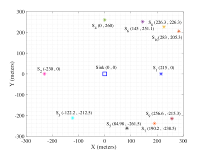
Figure 3: The considered WSN where the sink is located in the center and ${K=10}$ sensors are randomly placed. The coordinates of sensor $k$ is shown by $S_{k}(x_{k},y_{k})$.

VI-B Performance of the Proposed Dynamic Control Algorithm

In this section, we evaluate the performance of the proposed dynamic control algorithm (i.e., Algorithm 1) in terms of transmit power consumption and AoI of the sensors. To solve the optimization problem (21), we use Algorithm 2.

Fig. 4 illustrates the evolution of the average total transmit power for different values of parameter $V$ with maximum acceptable average AoI of sensors ${\Delta^{\text{max}}=4}$ and $N=10$ sub-channels. The figure shows that when $V$ increases, the average total transmit power decreases. This is because when $V$ increases, more emphasis is set to minimize the total transmit power in the objective function of optimization problem (21).

In addition, for the benchmarking, we consider a baseline policy that has a fixed sampling rate. The sampling rate is set as $1/7$, so that resulting average AoI of each sensor is equal to the maximum acceptable average AoI ${\Delta^{\text{max}}_{k}=\Delta^{\text{max}}=4,\forall k\in\mathcal{K}}$. The sampling schedule of the considered baseline method is presented in Table I. For this baseline policy, the sub-channel assignment and transmit power allocation are determined by the proposed methods in Sections V-A1 and V-A2, respectively. As it can be seen in Fig. 4, the proposed dynamic control algorithm achieves more than $60\leavevmode\nobreak\ \%$ saving in the average total transmit power compared to the baseline policy. This shows the advantage of the proposed dynamic control algorithm in optimizing the sampling process in contrast to relying on a pre-defined sampling schedule which enforces a sensor to transmit a status update even under a bad channel situation.

Table I: Sampling schedule of the considered fixed rate sampling policy of rate $1/7$

Time slot $t$	1	2	3	4	5	6	7	8	9	10	11	12	13	14	15	16
Sensor $k$ with $b_{k}(t)=1$	1	2	3	4	5, 6	7, 8	9, 10	1	2	3	4	5, 6	7, 8	9, 10	1	$\cdots$

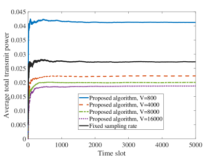
Figure 4: Evolution of the average total transmit power of the sensors for different values of $V$ with ${\Delta^{\text{max}}=4}$ and $N=10$. For comparison, a control policy with a fixed sampling rate is included as a baseline method.

Fig. 5 illustrates the trade-off between the average total transmit power and average backlogs of the virtual queues as a function of $V$ for ${\Delta^{\text{max}}=4}$ and $N=10$ sub-channels. As it can be seen, by increasing $V$ the average backlogs of the virtual queues increase and the average total transmit power decreases. This shows the inherent trade-off provided by the drift-plus-penalty method which was shown in Theorem 1. Moreover, the figure demonstrates that when $V$ is sufficiently large, increasing it further does not significantly reduce the power. This is visible in Fig. 4 as well.

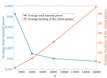
Figure 5: Trade-off between the average total transmit power of the sensors and average backlogs of the virtual queues as a function of $V$.

Fig. 6 illustrates the evolution of the average total transmit power for different numbers of sub-channels $N$ with ${\Delta^{\text{max}}=4}$ and $V=8000$. The figure shows that when $N$ increases, the average total transmit power decreases, as expected. This is because when $N$ increases, more sub-channels can be assigned to each sensor, and thus, one packet can be transmitted with less power. In addition, we can see that the effect of increasing the number of sub-channels from $N=6$ to $N=8$, and further to $N=10$, is more profound. This is because when there are fewer sub-channels than sensors, due to the orthogonality of the sub-channel assignment, all the sensors cannot be served in every slot and some sensors can get a sub-channel only after a few slots. Note that in order to meet the AoI constraint, the sensors may be enforced to transmit their sample even if the power consumption is excessive. On the other hand, increasing the number of sub-channels from $N=10$ to $N=12$ yields only negligible gain. This is because the greedy sub-channel assignment policy guarantees that each sensor will be assigned at least one sub-channel.

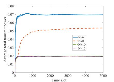
Figure 6: Evolution of the average total transmit power of the sensors for different numbers of sub-channels $N$ with ${\Delta^{\text{max}}=4}$ and $V=8000$.

Fig. 7 illustrates the evolution of the average total transmit power for different values of maximum AoI ${\Delta^{\text{max}}}$ with $N=10$ sub-channels and $V=8000$. The figure shows that when $\Delta^{\text{max}}$ decreases, the average total transmit power increases. This is because when $\Delta^{\text{max}}$ decreases, each sensor needs to take samples more frequently to satisfy constraint (7b).

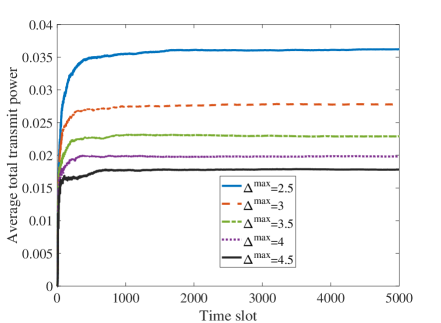
Figure 7: Evolution of the average total transmit power of the sensors for different values of $\Delta^{\text{max}}$ with $N=10$ and $V=8000$.

Fig. 8 depicts the average AoI for individual sensors as a function of $V$ for ${\Delta^{\text{max}}=4}$ and $N=10$ sub-channels. According to this figure, when $V$ increases, the average AoI of each sensor increases as well. This is because when $V$ increases, the backlogs of the virtual queues associated with the average AoI constraint (7b) increase. We can also observe that the average AoI of each sensor is always smaller than the maximum acceptable average AoI ${\Delta^{\text{max}}}$. This validates that the drift-plus-penalty method is able to meet the average constraint through enforcing the virtual queue stability. Moreover, we can see that a sensor that has a longer distance to the sink has higher average AoI. This is because a sensor far away from the sink must compensate for the large-scale fading by using more power, and thus, it samples rarely.

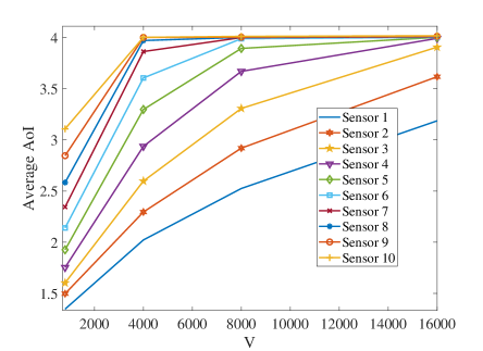
Figure 8: The average AoI of different sensors as a function of $V$ for ${\Delta^{\text{max}}=4}$ and $N=10$.

VI-C Performance of the Sub-Optimal Solution

To evaluate the optimality gap of the proposed sub-optimal solution for (21) presented in Algorithm 2, we compare the results obtained by the sub-optimal solution to those of the optimal solution calculated by the full exhaustive search method. In this regard, we consider a small setup with $K=5$ sensors $\{S_{1},\ldots,S_{5}\}$ (see Fig. 3) and ${N=5}$ sub-channels. The maximum acceptable average AoI of sensors is ${\Delta^{\text{max}}=4}$.

Fig. 9 illustrates the evolution of the average total transmit power for different values of $V$. Fig. 10 illustrates the trade-off between the average total transmit power of the sensors and average backlogs of the virtual queues as a function of $V$. Fig. 11 depicts the average AoI of different sensors as a function of $V$. Fig. 12 depicts the evolution of the average AoI of different sensors for $V=8000$. From these figures, we can see that the proposed sub-optimal solution provides a near-optimal solution for the optimization problem (21).

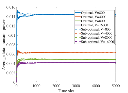
Figure 9: Evolution of the average total transmit power of the sensors for different values of $V$.

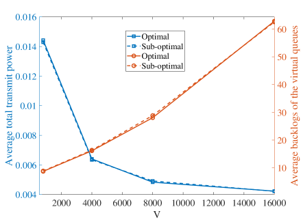
Figure 10: Trade-off between the average total transmit power and average backlogs of the virtual queues as a function of $V$.

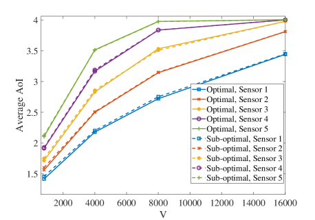
Figure 11: The average AoI of different sensors as a function of $V$.

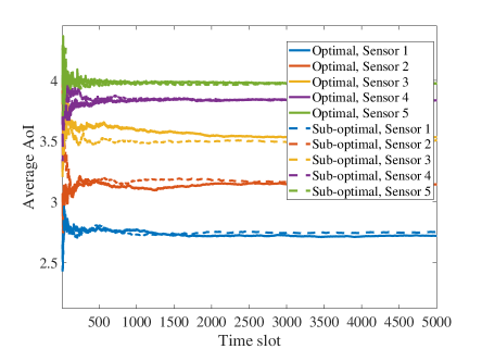
Figure 12: Evolution of the average AoI of different sensors for $V=8000$.

VII Conclusions

We considered a status update system consisting of a set of sensors and one sink. The sink controls the sampling process of the sensors in a way that it decides whether each sensor takes a sample or not at the beginning of each slot. The status update packets of the sensors are transmitted by sharing a set of orthogonal sub-channels in each slot. We formulated a problem to minimize the average total transmit power of sensors under the average AoI constraint for each sensor. To solve the proposed problem, we used the Lyapunov drift-plus-penalty method. This method provides a trade-off between the average total transmit power and the average AoI of the sensors. We conducted optimality analysis to study this trade-off. In the numerical results section, we showed the performance of the proposed dynamic solution algorithm in terms of transmit power consumption and AoI of sensors. The results showed that by using the proposed dynamic control algorithm more than $60\leavevmode\nobreak\ \%$ saving in the average total transmit power can be achieved compared to a baseline policy. In addition, we showed that the sub-optimal solution for the per-slot optimization problems provides a near-optimal solution.

The numerical results illustrated the inherent trade-off between the average AoI of the sensors and the average total transmit power that the Lyapunov drift-plus-penalty method brings in the system. This trade-off is adjusted by the penalty parameter $V$. A high value of $V$ is beneficial in that it enforces smaller transmit powers, yet at the cost of increasing the average AoI of each sensor. The results validated that, regardless of the value of $V$, the proposed drift-plus-penalty method met the time average AoI constraints through successfully enforcing the virtual queue stability. Regarding a selection of parameter $V$ in practice, we observed that when $V$ is sufficiently large, increasing it further does not significantly reduce the power.

References

- [1] M. Moltafet, M. Leinonen, M. Codreanu, and N. Pappas, “Power minimization in wireless sensor networks with constrained AoI using stochastic optimization,” in Proceedings of the Annual Asilomar Conference on Signals, Systems and Computers, Pacific Grove, USA, Nov. 3–6, 2019, pp. 406–410.
- [2] A. Kosta, N. Pappas, and V. Angelakis, Age of Information: A New Concept, Metric, and Tool. Foun. and Trends in Net., 2017, vol. 12, no. 3.
- [3] R. D. Yates and S. K. Kaul, “The age of information: Real-time status updating by multiple sources,” IEEE Trans. Inform. Theory, vol. 65, no. 3, pp. 1807–1827, Mar. 2019.
- [4] Y. Sun, I. Kadota, R. Talak, and E. Modiano, Age of Information: A New Metric For Information Freshness. Synthesis Lectures on Communication Networks, 2019, vol. 12, no. 2.
- [5] S. Kaul, R. Yates, and M. Gruteser, “Real-time status: How often should one update?” in Proceedings of the International Conference on Computer Communications (INFOCOM), Orlando, FL, USA, Mar. 25–30, 2012, pp. 2731–2735.
- [6] S. K. Kaul, R. D. Yates, and M. Gruteser, “Status updates through queues,” in Proceedings of the Conference on Information Sciences and Systems, Princeton, NJ, USA, Mar. 21–23, 2012, pp. 1–6.
- [7] S. Kaul, M. Gruteser, V. Rai, and J. Kenney, “Minimizing age of information in vehicular networks,” in Proceedings of the Communications Society Conference on Sensor, Mesh and Ad Hoc Communications and Networks, Salt Lake City, UT, USA, Jun. 27–30, 2011, pp. 350–358.
- [8] M. Costa, M. Codreanu, and A. Ephremides, “One the age of information in status update systems with packet management,” IEEE Trans. Inform. Theory, vol. 62, no. 4, pp. 1897–1910, Apr. 2016.
- [9] I. Kadota, A. Sinha, and E. Modiano, “Optimizing age of information in wireless networks with throughput constraints,” in Proceedings of the International Conference on Computer Communications (INFOCOM), Honolulu, HI, USA, Apr. 15–19, 2018, pp. 1844–1852.
- [10] Z. Chen, N. Pappas, E. Björnson, and E. G. Larsson, “Optimal control of status updates in a multiple access channel with stability constraints,” [Online]. https://arxiv.org/abs/1910.05144, 2019.
- [11] M. Moltafet, M. Leinonen, and M. Codreanu, “On the age of information in multi-source queueing models,” IEEE Trans. Commun., Early Access, [Online]. https://arxiv.org/abs/1911.07029v1, 2020.
- [12] M. Moltafet, M. Leinonen, and M. Codreanu, “Worst case age of information in wireless sensor networks: A multi-access channel,” IEEE Wireless Commun. Lett., vol. 9, no. 3, pp. 321–325, Mar. 2020.
- [13] M. Moltafet, M. Leinonen, and M. Codreanu, “Average age of information for a multi-source M/M/1 queueing model with packet management,” in Proceedings of the IEEE International Symposium on Information Theory, [Online]. https://arxiv.org/abs/2001.03959.pdf, 2020.
- [14] B. T. Bacinoglu and E. Uysal-Biyikoglu, “Scheduling status updates to minimize age of information with an energy harvesting sensor,” in Proceedings of the IEEE International Symposium on Information Theory, Aachen, Germany, Jun. 25–30, 2017.
- [15] D. Qiao and M. C. Gursoy, “Age-optimal power control for status update systems with packet-based transmissions,” IEEE Wireless Commun. Lett., vol. 8, no. 6, pp. 1604–1607, Jul. 2019.
- [16] R. V. Bhat, R. Vaze, and M. Motani, “Throughput maximization with an average age of information constraint in fading channels,” [Online]. https://arxiv.org/pdf/1911.07499.pdf, 2019.
- [17] X. Wu, J. Yang, and J. Wu, “Optimal status update for age of information minimization with an energy harvesting source,” IEEE Trans. Green Comm. Net., vol. 2, no. 1, pp. 193–204, Mar. 2018.
- [18] I. Krikidis, “Average age of information in wireless powered sensor networks,” IEEE Wireless Commun. Lett., vol. 8, no. 2, pp. 628–631, Apr. 2019.
- [19] I. Kadota, A. Sinha, and E. Modiano, “Scheduling algorithms for optimizing age of information in wireless networks with throughput constraints,” IEEE/ACM Trans. Networking, vol. 27, no. 4, pp. 1359–1372, Jun. 2019.
- [20] I. Kadota and E. Modiano, “Minimizing the age of information in wireless networks with stochastic arrivals,” IEEE Trans. Mobile Comput., Early Access, 2019.
- [21] E. Fountoulakis, N. Pappas, M. Codreanu, and A. Ephremides, “Optimal sampling cost in wireless networks with age of information constraints,” Toronto, ON, Canada,, Jul. 6–9, 2020, pp. 918–923.
- [22] V. Raghunathan, C. Schurgers, S. Park, and M. B. Srivastava, “Energy-aware wireless microsensor networks,” IEEE Signal Processing Mag., vol. 19, no. 2, pp. 40–50, Mar. 2002.
- [23] G. Anastasi, M. Conti, M. D. Francesco, and A. Passarella, “Energy conservation in wireless sensor networks: A survey,” Ad Hoc Netw., vol. 7, no. 3, pp. 537–568, May 2009.
- [24] M. Costa, M. Codreanu, and A. Ephremides, “Age of information with packet management,” in Proceedings of the IEEE International Symposium on Information Theory, Honolulu, HI, USA, Jun. 20–23, 2014, pp. 1583–1587.
- [25] E. Najm, R. Yates, and E. Soljanin, “Status updates through M/G/1/1 queues with HARQ,” in Proceedings of the IEEE International Symposium on Information Theory, Aachen, Germany, Jun. 25–30, 2017, pp. 131–135.
- [26] L. Huang and E. Modiano, “Optimizing age-of-information in a multi-class queueing system,” in Proceedings of the IEEE International Symposium on Information Theory, Hong Kong, China, Jun. 14–19, 2015, pp. 1681–1685.
- [27] M. Moltafet, M. Leinonen, and M. Codreanu, “Average AoI in multi-source systems with source-aware packet management,” (Under revision) IEEE Trans. Commun, [Online]: https://arxiv.org/pdf/2001.03959.pdf, 2020.
- [28] N. Akar, O. Dogan, and E. U. Atay, “Finding the exact distribution of (peak) age of information for queues of PH/PH/1/1 and M/PH/1/2 type,” IEEE Transactions on Communications, vol. 68, no. 9, pp. 5661–5672, Jun. 2020.
- [29] R. D. Yates, “Lazy is timely: Status updates by an energy harvesting source,” in Proceedings of the IEEE International Symposium on Information Theory, Hong Kong, China, Jun. 14–19, 2015, pp. 3008–3012.
- [30] B. T. Bacinoglu, E. T. Ceran, and E. Uysal-Biyikoglu, “Age of information under energy replenishment constraints,” in Proceedings of the IEEE Information Theory Workshop, San Diego, CA, USA, Feb. 1–6, 2015, pp. 25–31.
- [31] A. Arafa, J. Yang, S. Ulukus, and H. V. Poor, “Age-minimal transmission for energy harvesting sensors with finite batteries: Online policies,” IEEE Trans. Inform. Theory, vol. 66, no. 1, pp. 534–556, Sep. 2020.
- [32] R. D. Yates and S. K. Kaul, “Status updates over unreliable multiaccess channels,” in Proceedings of the IEEE International Symposium on Information Theory, Aachen, Germany, Jun. 25–30, 2017, pp. 331–335.
- [33] A. Kosta, N. Pappas, A. Ephremides, and V. Angelakis, “Age of information and throughput in a shared access network with heterogeneous traffic,” in Proceedings of the IEEE Global Telecommunication Conference, Abu Dhabi, United Arab Emirates, Dec. 9–13, 2018, pp. 1–6.
- [34] A. Maatouk, M. Assaad, and A. Ephremides, “On the age of information in a CSMA environment,” IEEE/ACM Trans. Net., Early Access 2020.
- [35] M. J. Neely, Stochastic Network Optimization With Application to Communication and Queueing Systems. Belmont, MA, USA: Morgan and Claypool, 2010.
- [36] L. Georgiadis, M. J. Neely, and L. Tassiulas, “Resource allocation and cross-layer control in wireless networks,” Found. Trends Netw., vol. 1, no. 1, pp. 1–144, Apr. 2006.
- [37] P. He and L. Zhao, “Generalized water-filling for sum power minimization with peak power constraints,” Nanjing, China, Oct. 15–17, 2015, pp. 1–5.