A parallel sampling algorithm for some nonlinear inverse problems

Abstract

We derive a parallel sampling algorithm for computational inverse problems that present an unknown linear forcing term and a vector of nonlinear parameters to be recovered. It is assumed that the data is noisy and that the linear part of the problem is ill-posed. The vector of nonlinear parameters ${\itbf m}$ is modeled as a random variable. A dilation parameter $\alpha$ is used to scale the regularity of the linear unknown and is also modeled as a random variable. A posterior probability distribution for $({\itbf m},\alpha)$ is derived following an approach related to the maximum likelihood regularization parameter selection [5]. A major difference in our approach is that, unlike in [5], we do not limit ourselves to the maximum likelihood value of $\alpha$. We then derive a parallel sampling algorithm where we alternate computing proposals in parallel and combining proposals to accept or reject them as in [4]. This algorithm is well-suited to problems where proposals are expensive to compute. We then apply it to an inverse problem in seismology. We show how our results compare favorably to those obtained from the Maximum Likelihood (ML), the Generalized Cross Validation (GCV), and the Constrained Least Squares (CLS) algorithms.

Keywords: Regularization, Linear and nonlinear inverse problems, Markov chains, Parallel computing, Elasticity equations in unbounded domains.

1 Introduction

Many physical phenomena are modeled by governing equations that depend linearly on some terms and non-linearly on other terms. For example, the wave equation may depend linearly on a forcing term and non-linearly on the medium velocity. This paper is on inverse problems where both a linear part and a nonlinear part are unknown. Such inverse problems occur in passive radar imaging, or in seismology where the source of an earthquake has to be determined (the source could be a point, or a fault) and a forcing term supported on that source is also unknown. This inverse problem is then linear in the unknown forcing term and nonlinear in the location of the source. The training phase of neural networks is another instance of an inverse problem where both linear and nonlinear unknowns occur. Most neural networks are based on linear combinations of basis functions depending on a few parameters and these parameters have to be determined by training the network on data, in other words by solving an inverse problem that combines linear and nonlinear unknowns [3].
Let us now formulate the inverse problem studied in this paper. Assume that after discretization a model leads to the relation

$${\itbf u}=A_{{\itbf m}}{\itbf g}+{\cal E},$$ (1.1)

where ${\itbf g}$ in $\mathbb{R}^{p}$ is a forcing term, ${\itbf m}$ in ${\cal B}\subset\mathbb{R}^{q}$ is a nonlinear parameter, $A_{\itbf m}$ is an $n\times p$ matrix depending continuously on the parameter ${\itbf m}$, ${\cal E}$ is a Gaussian random variable in $\mathbb{R}^{n}$ modeling noise, and ${\itbf u}$ in $\mathbb{R}^{n}$ is the resulting data for the inverse problem. For a fixed ${\itbf m}$, this is the same model that Golub et al. considered in [7]. In our case, our goal is to estimate the nonlinear parameter ${\itbf m}$ from ${\itbf u}$. We assume that the mapping from ${\cal B}$ to $\mathbb{R}^{n\times p}$, ${\itbf m}\rightarrow A_{\itbf m}$, is known, in other words, a model is known. We are interested in the challenging case where the following difficulties arise simultaneously:

1. the size $n\times p$ of the matrix $A_{{\itbf m}}$ is such that $n<<p$ (sparse data),

2. the singular values of $A_{{\itbf m}}$, $s_{1}\geq...\geq s_{n}>0$ are such that $s_{1}>>s_{n}>0$ ($A_{{\itbf m}}A_{{\itbf m}}^{\prime}$ is invertible but ill-conditioned),

3. ${\cal E}$ has zero mean and covariance $\sigma^{2}I_{n}$, but $\sigma$ is unknown.

Due to (i) and (ii), $\|A_{\itbf m}{\itbf g}-{\itbf u}\|$ can be made arbitrarily small for some ${\itbf g}$ in $\mathbb{R}^{p}$, thus the Variable Projection (VP) functional as defined in [6] can be minimized to numerical zero for all ${\itbf m}$ in the search set, and the Moore-Penrose inverse can not be used for this problem. Additionally, a numerical algorithm only based on minimizing a regularized functional may not adequately take into account the noise, which is amplified by ill-conditioning and nonlinear effects, and such an algorithm can easily get trapped in local minima. We thus set up the inverse problem consisting of finding ${\itbf m}$ from ${\itbf u}$ using (1.1) in a Bayesian framework where we seek to compute the posterior distribution of ${\itbf m}$. The inherent advantage of this probabilistic approach is that related Markov chains algorithms can avoid being trapped in local minima by occasionally accepting proposals of lower probability.
Stuart provided in [15] an extensive survey of probabilistic methods for inverse problems derived from PDE models and established connections between continuous formulations and their discrete equivalent. Particular examples found in [15] include an inverse problem for a diffusion coefficient, recovering the initial condition for the heat equation, and determining the permeability of subsurface rock using Darcy’s law. In the application to geophysics that we cover in section 3, ${\itbf g}$ models the slip on a fault, and ${\itbf m}$ is a parameter for modeling the piecewise linear geometry of a fault. The case of interest in this paper is particular due to the combination of the linear unknown ${\itbf g}$ which lies in $\mathbb{R}^{p}$, where $p$ is large, and the nonlinear unknown ${\itbf m}$ which lies in $\mathbb{R}^{q}$, with $q<<p$.

Tikhonov regularization may be used instead of the Moore-Penrose inverse to avoid a high norm or a highly oscillatory ${\itbf g}$ in (1.1). However, how regular solutions should be is unclear due to (iii). Accordingly, we introduce the regularized error functional,

$$\|A_{\itbf m}{\itbf g}-{\itbf u}\|^{2}+\alpha\|R{\itbf g}\|^{2},$$ (1.2)

where $R$ is an invertible $p$ by $p$ matrix and $\alpha>0$ is a scaling parameter. Typical choices for $R$ include the identity matrix and matrices derived from discretizing derivative operators. Without loss of generality, we can consider the functional

$$\|A_{\itbf m}{\itbf g}-{\itbf u}\|^{2}+\alpha\|{\itbf g}\|^{2},$$ (1.3)

in place of(1.2) by redefining $A_{\itbf m}$ as $A_{\itbf m}R^{-1}$.
Our solution method will rely on a Bayesian approach. Assuming that the prior of ${\itbf g}$ is also Gaussian, it is well-known that the functional (1.3) can be related to the probability density of ${\itbf u}$ knowing $\sigma,{\itbf m}$ and $\alpha$. However, $\sigma$ is unknown. We will use the Maximum Likelihood (ML) assumption to eliminate $\sigma$. As far as we know, this idea was first introduced (for linear problems only) in [5], but unlike in that reference, we do not eliminate $\alpha$. We let $\alpha$ be a random variable and thanks to Bayes’ theorem we find a formula for the probability density of $({\itbf m},\alpha)$ knowing ${\itbf u}$: this is stated in proposition 2.1. In section 2.4, this formula is used to build a parallel adaptive sampling algorithm to simulate the probability density of $({\itbf m},\alpha)$ knowing ${\itbf u}$. Finally we show in section 3 numerical simulations where this algorithm is applied to a particularly challenging inverse problem in geophysics. In this problem a fault geometry described by a nonlinear parameter ${\itbf m}$ in $\mathbb{R}^{6}$ has to be reconstructed from surface displacement data modeled by the vector ${\itbf u}$ in $\mathbb{R}^{n}$. The data is produced by a large slip field ${\cal G}$ modeled by a vector ${\itbf g}$ in $\mathbb{R}^{p}$. ${\itbf u}$ depends linearly on ${\itbf g}$ and this dependance can be expressed by a matrix $A_{{\itbf m}}$. In this simulation, the matrix $A_{{\itbf m}}$ is full since it is derived from convolution by a Green function. In addition, the entries of $A_{{\itbf m}}$ are particularly expensive to compute, which is a hallmark of problems involving half space elasticity and this application features all the difficulties (i), (ii), and (iii) listed above. This makes the VP functional method unsuitable, and it also renders classical minimization methods such as GCV, CLS, and ML much less accurate than our proposed method, as shown in section 3.3.

2 Solution method

2.1 The linear part of the inverse problem and selection methods for $\alpha$

There is a vast amount of literature on methods for selecting an adequate value for the regularization parameter $\alpha$, assuming that the nonlinear parameter ${\itbf m}$ is fixed. An account of most commonly used methods, together with error analysis, can be found in [18]. In this paper we review three such methods, that we later compare to our own algorithm. Throughout the rest of this paper, the Euclidean norm will be denoted by $\|.\|$ and the transpose of a matrix $M$ will be denoted by $M^{\prime}$.

2.1.1 Generalized cross validation (GCV)

The GCV method was first introduced and analyzed in [7]. The parameter $\alpha$ is selected by minimizing

$$\frac{\|(I_{n}-A_{\itbf m}(A_{\itbf m}^{\prime}A_{\itbf m}+\alpha I_{p})^{-1}A_{\itbf m}^{\prime}){\itbf u}\|^{2}}{\mbox{tr }(I_{n}-A_{\itbf m}(A_{\itbf m}^{\prime}A_{\itbf m}+\alpha I_{p})^{-1}A_{\itbf m}^{\prime})^{2}},$$ (2.1)

where tr is the trace. Let $\alpha_{GCV}$ be the value of $\alpha$ which minimizes (2.1). Golub et al. proved in [7] that as a function of $\alpha$, the expected value of $\|A_{\itbf m}{\itbf g}-A_{\itbf m}(A_{\itbf m}^{\prime}A_{\itbf m}+\alpha I_{p})^{-1}A_{\itbf m}^{\prime}{\itbf u}\|^{2}$ which can be thought of as an indicator of fidelity of the pseudo-solution $(A_{\itbf m}^{\prime}A_{\itbf m}+\alpha R^{\prime}R)^{-1}A_{\itbf m}^{\prime}{\itbf u}$ is approximately minimized at $\alpha=\alpha_{GCV}$ as $n\rightarrow\infty$. Although the GCV method enjoys this remarkable asymptotic property and does not require knowing $\sigma^{2}$, many authors have noted that determining the minimum of (2.1) in practice can be costly and inaccurate as in practical situations the quantity in (2.1) is flat near its minimum for a wide range of values of $\alpha$ [16, 17].

2.1.2 Constrained least square (CLS)

This method, also called the discrepancy principle [11, 18], advocates choosing a value for $\alpha$ such that

$$\|{\itbf u}-A_{\itbf m}(A_{\itbf m}^{\prime}A_{\itbf m}+\alpha I_{p})^{-1}A_{\itbf m}^{\prime}{\itbf u}\|^{2}=n\sigma^{2}.$$ (2.2)

Clearly, applying this method requires knowing $\sigma^{2}$ or at least some reasonable approximation of its value. Even if $\sigma^{2}$ is known, this method leads to solutions that are in general overly smooth, [5, 18].

2.1.3 Maximum likelihood (ML)

To the best of our knowledge the ML method was first proposed in [5]. It relies on the fundamental assumption that the prior of $\alpha^{\frac{1}{2}}{\itbf g}$ is also normal with zero mean and covariance $\sigma^{2}I_{p}$. The likelihood of the minimizer of (1.3) knowing $\sigma$ and $\alpha$ is then maximized for all $\alpha>0$, $\sigma>0$. Galatsanos and Katsaggelos showed in [5] that equivalently the expression

$$\frac{{\itbf u}^{\prime}(I_{n}-A_{\itbf m}(A_{\itbf m}^{\prime}A_{\itbf m}+\alpha I_{p})^{-1}A_{\itbf m}^{\prime}){\itbf u}}{(\det(I_{n}-A_{\itbf m}(A_{\itbf m}^{\prime}A_{\itbf m}+\alpha I_{p})^{-1}A_{\itbf m}^{\prime}))^{1/n}}\,,$$ (2.3)

has to be minimized for all $\alpha>0$, which does not require knowing $\sigma^{2}$.

2.2 A sampling algorithm for computing the posterior of $({\itbf m},\alpha)$

In this section we generalize the ML method recalled in section 2.1.3 to problems depending nonlinearly on the random variable ${\itbf m}$, while refraining from only retaining the maximum likelihood value of $\alpha$.

Proposition 2.1

Assume that

1. ${\itbf u}$, ${\itbf g}$, ${\itbf m}$ and $\alpha$ are random variables in $\mathbb{R}^{n},\mathbb{R}^{p},{\cal B}\subset\mathbb{R}^{q},(0,\infty)$, respectively,

2. $({\itbf m},\alpha)$ has a known prior distribution denoted by $\rho_{pr}({\itbf m},\alpha)$,

3. $A_{{\itbf m}}$ is an $n$ by $p$ matrix which depends continuously on ${\itbf m}$,

4. ${\cal E}$ is an $n$ dimensional normal random variable with zero mean and covariance $\sigma^{2}I_{n}$,

5. relation (1.1) holds,

6. the prior of $\alpha^{\frac{1}{2}}{\itbf g}$ is a normal random variable with zero mean and covariance $\sigma^{2}I_{p}$.

Let $\rho({\itbf u}|\sigma,{\itbf m},\alpha)$ be the conditional probability density of ${\itbf u}$ knowing $\sigma,{\itbf m},\alpha$. As a function of $\sigma>0$, $\rho({\itbf u}|\sigma,{\itbf m},\alpha)$ achieves a unique maximum at

$$\sigma_{max}^{2}=\frac{1}{n}(\alpha\|{\itbf g}_{min}\|^{2}+\|{\itbf u}-A_{\itbf m}{\itbf g}_{min}\|^{2}),$$ (2.4)

where ${\itbf g}_{min}=(A_{\itbf m}^{\prime}A_{\itbf m}+\alpha I_{p})^{-1}A_{\itbf m}^{\prime}{\itbf u}$ is the minimizer of (1.3). Fixing $\sigma=\sigma_{max}$, the probability density of $({\itbf m},\alpha)$ knowing ${\itbf u}\neq 0$ is then given, up to a multiplicative constant, by the formula

$$\rho({\itbf m},\alpha|{\itbf u})\propto\det(\alpha^{-1}A_{\itbf m}^{\prime}A_{\itbf m}+I_{p})^{-\frac{1}{2}}(\alpha\|{\itbf g}_{min}\|^{2}+\|{\itbf u}-A_{\itbf m}{\itbf g}_{min}\|^{2})^{-\frac{n}{2}}\rho_{pr}({\itbf m},\alpha).$$ (2.5)

Note that Galatsanos and Katsaggelos give a proof in [5] of a closely related result, but our context is somehow different. Our matrix $A_{\itbf m}$ is rectangular and depends continuously and non-linearly on the random variable ${\itbf m}$. In the present case, a similar argument can be carried out noting that thanks to assumption H6., the marginal probability density of ${\itbf u}$ knowing $\sigma,{\itbf m},\alpha$ can be computed and equals, using the minimizer ${\itbf g}_{min}=(A_{\itbf m}^{\prime}A_{\itbf m}+\alpha I_{p})^{-1}A_{\itbf m}^{\prime}{\itbf u}$ of (1.3),

$$(\frac{1}{2\pi\sigma^{2}})^{\frac{n}{2}}\alpha^{\frac{p}{2}}\exp(-\frac{\alpha}{2\sigma^{2}}\|{\itbf g}_{min}\|^{2}-\frac{1}{2\sigma^{2}}\|{\itbf u}-A_{\itbf m}{\itbf g}_{min}\|^{2})(\det(A_{\itbf m}^{\prime}A_{\itbf m}+\alpha I_{p}))^{-\frac{1}{2}},$$

which is in turn maximized for $\sigma$ in $(0,\infty)$. This yields formula (2.4). Formula (2.5) follows from there.

Note that the fundamental assumption H6. was introduced in [5] and can be thought of as a way of restoring a balance between reconstruction fidelity (first term in (1.3)) and regularity requirements (second term in (1.3)). We note that the right hand side of (2.5) can be related to the ML ratio (2.3), first because as ${\itbf g}_{min}=(A_{\itbf m}^{\prime}A_{\itbf m}+\alpha I_{p})^{-1}A_{\itbf m}^{\prime}{\itbf u}$, a simple calculation will show that

$$\|{\itbf u}-A_{\itbf m}{\itbf g}_{min}\|^{2}+\alpha\|{\itbf g}_{min}\|^{2}={\itbf u}^{\prime}(I_{n}-A_{\itbf m}(A_{\itbf m}^{\prime}A_{\itbf m}+\alpha I_{p})^{-1}A_{\itbf m}^{\prime}){\itbf u},$$

and second because of the identity

$$(\det(\alpha^{-1}A_{\itbf m}^{\prime}A_{\itbf m}+I_{p}))^{-1}=\det(I_{n}-A_{\itbf m}(A_{\itbf m}^{\prime}A_{\itbf m}+\alpha I_{p})^{-1}A_{\itbf m}^{\prime}).$$ (2.6)

which is shown in Appendix A. Next it is important to note that, as explained in Appendix A,

$$I_{n}-A_{\itbf m}(A_{\itbf m}^{\prime}A_{\itbf m}+\alpha I_{p})^{-1}A_{\itbf m}^{\prime}=(I_{n}+\alpha^{-1}A_{\itbf m}A_{\itbf m}^{\prime})^{-1}.$$

Since $n<<p$, this is particularly helpful in numerical calculations, and it allows to use the formula ${\itbf u}^{\prime}(I_{n}+\alpha^{-1}A_{\itbf m}A_{\itbf m}^{\prime})^{-1}{\itbf u}$ to compute $\|{\itbf u}-A_{\itbf m}{\itbf g}_{min}\|^{2}+\alpha\|{\itbf g}_{min}\|^{2}$. Introducing ${\itbf g}_{min}$ is helpful, however, for comparing the solution method developed in this paper to classical variational regularization methods see, section 1.3 in [18].

2.3 Single processor algorithm

Based on (2.5), we define the non-normalized distribution

$${\cal R}({\itbf m},\alpha)=\det(\alpha^{-1}A_{\itbf m}^{\prime}A_{\itbf m}+I_{p})^{-\frac{1}{2}}(\alpha\|{\itbf g}_{min}\|^{2}+\|{\itbf u}-A_{\itbf m}{\itbf g}_{min}\|^{2})^{-\frac{n}{2}}\rho_{pr}({\itbf m},\alpha).$$ (2.7)

We use the standard notations ${\cal N}(\mu,\textsf{$\Sigma$})$ for a normal distribution with mean $\mu$ and covariance $\Sigma$, ${\cal}U(0,1)$ for a uniform distribution in the interval $(0,1)$. The algorithm starts from a point $({\itbf m}_{1},\alpha_{1})$ in $\mathbb{R}^{q+1}$ such that $\rho_{pr}({\itbf m}_{1},\alpha_{1})>0$ and an initial covariance matrix $\Sigma_{0}$ obtained from the prior distribution. A good choice of the initial point $({\itbf m}_{1},\alpha_{1})$ may have a strong impact on how many sampling steps are necessary. A poor choice may result in a very long ”burn in” phase where the random walk is lost in a low probability region. How to find a good starting point $({\itbf m}_{1},\alpha_{1})$ depends greatly on the application, so we will discuss that issue in a later section where we cover a specific example. Our basic single processor algorithm follows the well established adaptive MCMC propose/accept/reject algorithm [13]. Let $\beta_{j}$ be a decreasing sequence in $(0,1)$ which converges to 0. This sequence is used to weigh a convex combination between the initial covariance $\Sigma_{0}$ and the covariance $\Sigma$ learned from sampling. The updating of $\Sigma$ need not occur at every step. Let $N$ be the total number of steps and $N^{\prime}$ the number of steps between updates of $\Sigma$. We require that $1<N^{\prime}<N$. Finally, the covariance for the proposals is adjusted by a factor of $(2.38)^{2}(q+1)^{-1}$ as recommended in [13, 14]. It was shown in [14] that this scaling leads to an optimal acceptance rate.

Single processor sampling algorithm

1. Start from a point $({\itbf m}_{1},\alpha_{1})$ in $\mathbb{R}^{q+1}$ and set $\Sigma=\Sigma_{0}$.

2. for $j=2$ to $N$ do:

   1. if $j$ is a multiple of $N^{\prime}$ update the covariance $\Sigma$ by using the points $({\itbf m}_{k},\alpha_{k}),1\leq k\leq j-1$,

   2. draw $({\itbf m}^{*},\alpha^{*})$ from $({\itbf m}_{j-1},\alpha_{j-1})+(1-\beta_{j}){\cal N}(0,(2.38)^{2}(q+1)^{-1}\textsf{$\Sigma$})+\beta_{j}{\cal N}(0,(2.38)^{2}(q+1)^{-1}\textsf{ $\Sigma_{0}$})$,

   3. compute ${\cal R}({\itbf m}^{*},\alpha^{*})$,

   4. draw $u$ from ${\cal U}(0,1)$,

   5. if $u<\frac{{\cal R}({\itbf m}^{*},\alpha^{*})}{{\cal R}({\itbf m}_{j-1},\alpha_{j-1})}$ set $({\itbf m}_{j},\alpha_{j})=({\itbf m}^{*},\alpha^{*})$, else set $({\itbf m}_{j},\alpha_{j})=({\itbf m}_{j-1},\alpha_{j-1})$.

2.4 Parallel algorithm

Let $N_{par}$ be the number of processing units. A straightforward way of taking advantage of multiple processors is to generate $N_{par}$ separate chains of samples using the single processor algorithm described in section 2.3 and then concatenate them. However, computations can be greatly accelerated by analyzing the proposals produced by the chains in aggregate [4, 9]. While in section 2.3 $({\itbf m}_{j},\alpha_{j},)$ was a $q+1$ dimensional vector, here we set $\textsf{M}_{j}$ to be a $q+1$ by $N_{par}$ matrix where the $k$-th column will be denoted by $\textsf{M}_{j}(k)$ and is a sample of the random variable $({\itbf m},\alpha)$, $k=1,...,N_{par}$. Next, if $j\geq 2$, we assemble an $N_{par}+1$ by $N_{par}+1$ transition matrix $T$ from the computed non-normalized densities ${\cal R}(\textsf{M}_{j-1}(N_{par}))$ and ${\cal R}(\textsf{M}^{*}(k))$, $k=1,...,N_{par}$, where $\textsf{M}^{*}$ is the proposal. Let ${\itbf w}$ be the vector in $\mathbb{R}^{N_{par}+1}$ with coordinates

$${\itbf w}=\big{(}{\cal R}(\textsf{M}_{j-1}(N_{par})),{\cal R}(\textsf{M}^{*}(1)),...,{\cal R}(\textsf{M}^{*}(N_{par}))\big{)}.$$

The entries of the transition matrix $T$ are given by the following formula [4],

$$T_{k,l}=\displaystyle\left\{\begin{array}[]{l}\displaystyle\frac{1}{N_{par}}\min\{1,\frac{w_{l}}{w_{k}}\},\mbox{ if }k\neq l,\\ \displaystyle 1-\sum_{1\leq l\leq N_{par}+1,l\neq k}T_{k,l},\mbox{ if }k=l.\end{array}\right.$$ (2.10)

Note that for $k=1,...,N_{par}+1$ the row $T_{k,1},...,T_{k,N_{par}+1}$ defines a discrete probability distribution on $\{1,...,N_{par}+1\}$.

Parallel sampling algorithm

1. Start from a point $({\itbf m}_{1},\alpha_{1})$ in $\mathbb{R}^{q+1}$ and set $\Sigma=\Sigma_{0}$. Set the $N_{par}$ columns of $\textsf{M}_{1}$ to be equal to $({\itbf m}_{1},\alpha_{1})$.

2. for $j=2$ to $N$ do:

   1. if $j$ is a multiple of $N^{\prime}$ update the covariance $\Sigma$ by using the points $\textsf{M}_{k}(l),1\leq k\leq j-1,1\leq l\leq N_{par}$,

   2. for $k=1$ to $N_{par}$, draw the proposals $\textsf{M}^{*}(k)$ from $\textsf{M}_{j-1}(k)+(1-\beta_{j}){\cal N}(0,(2.38)^{2}(q+1)^{-1}\textsf{$\Sigma$})+\beta_{j}{\cal N}(0,(2.38)^{2}(q+1)^{-1}\textsf{$\Sigma_{0}$})$,

   3. compute in parallel ${\cal R}(\textsf{M}^{*}(k))$, $k=1,...,N_{par}$,

   4. assemble the $N_{par}+1$ by $N_{par}+1$ transition matrix $T$ as indicated above,

   5. for $k=2,...,N_{par}+1$ draw an integer $p$ in $\{1,...,N_{par}+1\}$ using the probability distribution $T_{k,1},...,T_{k,N_{par}+1}$; if $p=1$ set $\textsf{M}_{j}(k-1)=\textsf{M}_{j-1}(N_{par})$ (reject), otherwise set $\textsf{M}_{j}(k-1)=\textsf{M}^{*}(p-1)$ (accept).

Note that this parallel algorithm is especially well suited to applications where computing the non-normalized density ${\cal R}({\itbf m},\alpha)$ is expensive. In that case, even the naive parallel algorithm where $N_{par}$ separate chains are computed in parallel will be about $N_{par}$ times more efficient than the single processor algorithm. The parallel algorithm presented in this section is in fact even more efficient due to superior mixing properties and sampling performance: the performance is not overly sensitive to tuning of proposal parameters [4].

3 Application to the fault inverse problem in seismology and numerical simulations

Using standard rectangular coordinates, let ${\itbf x}=(x_{1},x_{2},x_{3})$ denote elements of $\mathbb{R}^{3}$. We define $\mathbb{R}^{3-}$ to be the open half space $x_{3}<0$. We use the equations of linear elasticity with Lamé constants $\lambda$ and $\mu$ such that $\lambda>0$ and $\lambda+\mu>0$. For a vector field ${\cal V}=({\cal V}_{1},{\cal V}_{2},{\cal V}_{3})$, the stress vector in the direction ${\itbf e}\in\mathbb{R}^{3}$ will be denoted by

$$T_{\itbf e}{\cal V}=\sum_{j=1}^{3}\left(\lambda\,\mbox{div }{\cal V}\,\delta_{ij}+\mu\,(\partial_{i}{\cal V}_{j}+\partial_{j}{\cal V}_{i})\right)e_{j}.$$

Let $\Gamma$ be a Lipschitz open surface which is strictly included in $\mathbb{R}^{3-}$, with normal vector ${\itbf n}$. We define the jump $\mbox{$[$}{\cal V}\mbox{$]$}$ of the vector field ${\cal V}$ across $\Gamma$ to be

$$\mbox{$[$}{\cal V}\mbox{$]$}({\itbf x})=\lim_{h\rightarrow 0^{+}}{\cal V}({\itbf x}+h{\itbf n})-{\cal V}({\itbf x}-h{\itbf n}),$$

for ${\itbf x}$ in $\Gamma$, if this limit exists. Let ${\cal U}$ be the displacement field solving

$$\mu\Delta{\cal U}+(\lambda+\mu)\nabla\mbox{div }{\cal U}=0\mbox{ in }\mathbb{R}^{3-}\setminus\Gamma,$$ (3.1)

$$T_{{\itbf e}_{3}}{\cal U}=0\mbox{ on the surface }x_{3}=0,$$ (3.2)

$$T_{{\itbf n}}{\cal U}\mbox{ is continuous across }\Gamma,$$ (3.3)

$$\mbox{$[$}{\cal U}\mbox{$]$}={\cal G}\mbox{ is a given jump across }\Gamma,$$ (3.4)

$${\cal U}({\itbf x})=O(\frac{1}{|{\itbf x}|^{2}}),\nabla{\cal U}({\itbf x})=O(\frac{1}{|{\itbf x}|^{3}}),\mbox{ uniformly as }|{\itbf x}|\rightarrow\infty,$$ (3.5)

where ${\itbf e}_{3}$ is the vector $(0,0,1)$.

Let $D$ be a bounded domain in $\mathbb{R}^{3-}$ with Lipschitz boundary $\partial D$ containing $\Gamma$. Let $\widetilde{H}^{\frac{1}{2}}(\Gamma)^{2}$ be the space of restrictions to $\Gamma$ of tangential fields in $H^{\frac{1}{2}}(\partial D)^{2}$ supported in $\overline{\Gamma}$. In [21], we defined the functional space ${\bf S}$ of vector fields ${\cal V}$ defined in $\mathbb{R}^{3-}\setminus{\overline{\Gamma}}$ such that $\nabla{\cal V}$ and $\displaystyle\frac{{\cal V}}{(1+r^{2})^{\frac{1}{2}}}$ are in $L^{2}(\mathbb{R}^{3-}\setminus{\overline{\Gamma}})$ and we proved the following existence and uniqueness result.

Theorem 3.1

Let ${\cal G}$ be in $\widetilde{H}^{\frac{1}{2}}(\Gamma)^{2}$. The problem (3.1-3.4) has a unique solution in ${\bf S}$. In addition, the solution ${\cal U}$ satisfies the decay conditions (3.5).

Can both ${\cal G}$ and $\Gamma$ be determined from the data ${\cal U}$ given only on the plane $x_{3}=0$? The following Theorem shown in [21] asserts that this is possible if the data is known on a relatively open set of the plane $x_{3}=0$.

Theorem 3.2

Let $\Gamma_{1}$ and $\Gamma_{2}$ be two connected open surfaces that are unions of two polygons. For $i$ in $\{1,2\}$, assume that ${\cal U}^{i}$ solves (3.1-3.5) for $\Gamma_{i}$ in place of $\Gamma$ and ${\cal G}^{i}$, a tangential field in $\tilde{H}^{\frac{1}{2}}(\Gamma_{i})^{2}$, in place of ${\cal G}$. Assume that ${\cal G}^{i}$ has full support in $\Gamma_{i}$, that is, $\mbox{supp }{\cal G}_{i}=\overline{\Gamma_{i}}$. Let $V$ be a non empty open subset in $\{x_{3}=0\}$. If ${\cal U}^{1}$ and ${\cal U}^{2}$ are equal in $V$, then $\Gamma_{1}=\Gamma_{2}$ and ${\cal G}^{1}={\cal G}^{2}$.

Theorems 3.1 and 3.2 were proved in [21] for media with constant Lamé coefficients. Later, in [2], the direct problem (3.1-3.4) was analyzed under weaker regularity conditions for ${\cal U}$ and ${\cal G}$. In [1], the direct problem (3.1-3.4) was proved to be uniquely solvable in case of piecewise Lipschitz coefficients and general elasticity tensors. Both [1] and [2] include a proof of uniqueness for the fault inverse problem under appropriate assumptions. In our case, the solution ${\cal U}$ to problem (3.1-3.4) can also be written out as the convolution on $\Gamma$

$${\cal U}({\itbf x})=\int_{\Gamma}{\itbf H}({\itbf x},{\itbf y},{\itbf n}){\cal G}({\itbf y})\,d\sigma({\itbf y}),$$ (3.6)

where ${\itbf H}$ is the Green’s tensor associated to the system (3.1-3.5), and ${\itbf n}$ is the normal to $\Gamma$. The practical determination of this adequate half space Green’s tensor ${\itbf H}$ was first studied in [12] and later, more rigorously, in [19]. Due to formula (3.6) we can define a continuous mapping ${\cal M}$ from tangential fields ${\cal G}$ in $H^{1}_{0}(\Gamma)^{2}$ to surface displacement fields ${\cal U}(x_{1},x_{2},0)$ in $L^{2}(V)$. Theorem 3.2 asserts that this mapping is injective, so an inverse operator can be defined. It is well known, however, that such an operator ${\cal M}$ is compact, therefore its inverse is unbounded.

We assume here that $n$ is a multiple of three since three-dimensional displacements are measured. Let $O_{j},j=1,..,\frac{n}{3}$ be the points on the plane $x_{3}=0$ where measurements are collected, giving rise to a data vector ${\itbf u}$ in $\mathbb{R}^{n}$. In our numerical simulations, we assume that $\Gamma$ is made up of two contiguous quadrilaterals, and that $\Gamma$ is the image by a piecewise affine function of the square $S=[-100,200]\times[-100,200]$ in the $x_{1}x_{2}$ plane. Applying a change of variables in the integral given by (3.6), the field ${\cal G}$ may be assumed to be defined on $S$ and the integral itself becomes an integral on $S$. We use a regular $m\times m$ grid of points on $S$, thus we set $p=m^{2}$. The points on this grid are then labeled $Q_{k},k=1,..,p$. Let $\tilde{Q}_{k}$ be the points on $\Gamma$ with same $x_{1}$ and $x_{2}$ coordinates as $Q_{k}$, $k=1,..,p$: ${\itbf g}$ in $\mathbb{R}^{p}$ is used to approximate ${\cal G}$ at these points. The Green tensor ${\itbf H}$ is evaluated at $({\itbf x},{\itbf y})=(O_{j},\tilde{Q}_{k}),j=1,..,\frac{n}{3},k=1,..,p$, and the integral in (3.6) is approximated by quadrature. Since $\Gamma$ is the image of $S$ by a piecewise affine function, assuming that $\Gamma$ is made up of two contiguous quadrilaterals, it can be defined by a parameter ${\itbf m}$ in $\mathbb{R}^{6}$. We then write the discrete equivalent of the right hand side of formula (3.6) as the matrix-vector product $A_{\itbf m}{\itbf g}$, where ${\itbf g}$ in $\mathbb{R}^{p}$ is the discrete analog of ${\cal G}$ and multiplying by the matrix $A_{\itbf m}$ is the discrete analog of applying the convolution product of ${\cal G}$ against ${\itbf H}$ over $\Gamma$. Taking into account measurement errors, we arrive at the formulation (1.1). In the simulations shown in this paper the size of the matrix $A_{\itbf m}$ is $n\times p\sim 500\times 2500$. The singular values of $A_{\itbf m}$ decay fast (this is due to the fast decay of the singular values of the compact operator ${\cal M}$, see [10]), so even choosing a coarser grid on $\Gamma$ which would make $p\leq n$ would still result in an ill-conditioned matrix $A_{\itbf m}^{\prime}A_{\itbf m}$. In Figure 1 we plot the singular values of $A_{\itbf m}$ for the particular value of ${\itbf m}$ used to generate the direct data for the inverse problem used for illustration in the next section. A similar fast decay of these singular values is observed for all ${\itbf m}$ in the support of its prior.

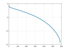
Figure 1: The decimal logarithm of the singular values of $A_{\itbf m}$ with $n\times p=585\times 10201$, and ${\itbf m}$ given by (3.7).

Another practical aspect of the matrix $A_{m}$ is that it is full (as is usually the case in problems derived from integral operators) and its entries are expensive to compute (this is due to the nature of the half space elastic Green tensor) [19]. However, great gains can be achieved by applying array operations thus taking advantage of multithreading. The matrix $R$ used to regularize ${\itbf g}$ as in (1.2) is based on derivatives in the $x_{1}$ and $x_{2}$ directions. We can find two $p$ by $p$ permutation matrices $P_{D}$ and $P_{E}$ satisfying $D=P_{D}^{-1}MP_{D}$, $E=P_{E}^{-1}MP_{E}$, where $M$ is block-diagonal with each block of size $m\times m$ given by

$$\begin{bmatrix}1&-1&0&0&\cdots&0\\ 0&1&-1&0&\cdots&0\\ \vdots&\ddots&\ddots&\ddots&\ddots&\vdots\\ \vdots&\ddots&\ddots&\ddots&\ddots&0\\ 0&\cdots&\cdots&0&1&-1\\ 0&\cdots&\cdots&\cdots&0&1\end{bmatrix},$$

such that $D$ is the discrete analog of a derivative operator in the $x_{1}$ direction and $E$ is the discrete analog of the derivative operator in the $x_{2}$ direction. Note that $\|D\|\leq 2$, $\|E\|\leq 2$, and $\|D^{-1}\|\leq p$, $\|E^{-1}\|\leq p$, in matrix 2 norm. We then define $R$ to be a matrix such that $R^{\prime}R=D^{\prime}D+E^{\prime}E$. Evaluating $R$ is unnecessary since only $R^{\prime}R$ is used in computations. For efficiency, it is advantageous not to evaluate the matrix product $A_{\itbf m}R^{-1}$ to reduce (1.2) to (1.3). Instead, we evaluate and store $R^{\prime}R$ and we use an iterative solver to evaluate ${\itbf g}_{min}=(A_{\itbf m}^{\prime}A_{\itbf m}+\alpha R^{\prime}R)^{-1}A_{\itbf m}^{\prime}{\itbf u}$. We coded the function ${\itbf g}\rightarrow(A_{\itbf m}^{\prime}A_{\itbf m}+\alpha R^{\prime}R){\itbf g}$ without evaluating the matrix product $A_{\itbf m}^{\prime}A_{\itbf m}$.

3.1 Construction of the data

We consider data generated in a configuration closely related to studies involving field data for a particular region and a specific seismic event [20, 22]. In those studies, simulations involved only planar faults, while here we examine the case of fault geometries defined by pairs of contiguous quadrilaterals. Obviously, reconstructing finer geometries as considered here requires many more measurement points than used in [20, 22] (11 points in [20] versus 195 points here). The higher number of measurement points used here allows us to reconstruct $\Gamma$ even if the data is very noisy, at the cost of finding large standard deviations. In our model, the geometry of $\Gamma$ is determined from ${\itbf m}$ in $\mathbb{R}^{6}$ in the following way:

• $\Gamma$ is beneath the square $[-100,200]\times[-100,200]$

• Let $P_{1}$ be the point $(-100,-100,m_{1})$

• Let $P_{2}$ be the point $(-100,m_{2},m_{3})$, such that $-100<m_{2}<200$

• Let $P_{3}$ be the point $(200,m_{4},m_{5})$, such that $-100<m_{4}<200$

• Let $P_{4}$ be the point $(200,200,m_{6})$

• Let $P_{5}$ be the point in the plane $P_{1}P_{2}P_{3}$ with $x_{1},x_{2}$ coordinates $(200,-100)$

• Let $P_{6}$ be the point in the plane $P_{2}P_{3}P_{4}$ with $x_{1},x_{2}$ coordinates $(-100,200)$

• Form the union of the two quadrilaterals $P_{1}P_{2}P_{3}P_{5}$ and $P_{2}P_{3}P_{4}P_{6}$ and discard the part where $x_{3}\geq 0$ to obtain $\Gamma$

For generating forward data we picked the particular values

$$m=(24,145,-40,8,-40-50).$$ (3.7)

In Figure 2, we show a sketch of $\Gamma$ viewed from above with the points $P_{1},P_{2},P_{3},P_{4},P_{5},P_{6}$, and we also sketch $\Gamma$ in three dimensions.

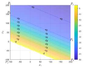
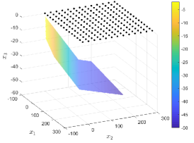
Figure 2: The piecewise planar surface $\Gamma$. Depths are indicated by color bars. Top graph: view of $\Gamma$ from above with the six points $P_{1},P_{2},P_{3},P_{4},P_{5},P_{6}$ and contour lines of same depth. Bottom graph: a three dimensional rendition of $\Gamma$. The measurement points are on the surface $x_{3}=0$ and are indicated by black dots.

In Figure 3, we show a graph of the slip field ${\cal G}$ as a function of $(x_{1},x_{2})$ (recall that this slip field is supported on $\Gamma$ so Figure 3 shows a projection of ${\cal G}$ on a horizontal plane). We model a slip of pure thrust type, meaning that slip occurs in the direction of steepest descent, so only the norm of ${\cal G}$ is graphed.

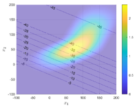
Figure 3: The slip field $\cal{G}$. We are using a pure thrust model, that is, the direction of the slip is in the line of steepest descent, only the modulus of $\cal{G}$ is shown. The colorbar shows the scale for the modulus of $\cal{G}$. As previously, lines of equal depth on $\Gamma$ are indicated.

We used this slip $\cal{G}$ to compute the resulting surface displacements thanks to formula (3.6) where we discretized the integral on a fine mesh. The data for the inverse problem is the noise-free three dimensional displacements ${\itbf u}_{free}$ at the measurement points shown in Figure 2 to which we added Gaussian noise with zero mean and covariance $\sigma^{2}I$ to obtain ${\itbf u}$. We consider two scenarios: lower and higher noise. In the lower noise scenario $\sigma$ was set to be equal to 5% of the maximum of the absolute values of the components of ${\itbf u}_{free}$ (in other words, 5% of $\|{\itbf u}_{free}\|_{\infty}$). For the particular realization used in solving the inverse problem, this led to a relative error in Euclidean norm of about 7% (in other words, for this particular realization ${\cal E}(\omega)$ of the noise, $\|{\cal E}(\omega)\|/\|{\itbf u}_{free}\|$ was about 0.07, where $\|.\|$ is the Euclidean norm). In the higher noise case scenario $\sigma$ was set to be equal to 25% of the maximum of the absolute values of the components of ${\itbf u}$ (in other words, 25% of $\|{\itbf u}_{free}\|_{\infty}$). This time, this led to a relative error in Euclidean norm of about 37%. Both realizations are shown in Figure 4 (only the horizontal components are sketched for the sake of brevity). All lengthscales used in these simulation are in line with the canonical example from geophysics provided by the 2007 Guerrero slow slip event [20, 22]. In particular, $x_{1},x_{2},x_{3}$ are thought of as given in kilometers and ${\itbf g}$ and ${\itbf u}$ in meters. In real life applications, the noise level is likely to lie somewhere between the low noise scenario and high noise scenario considered here.

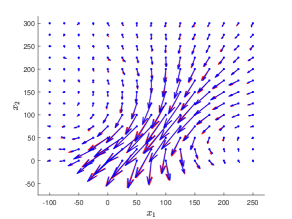
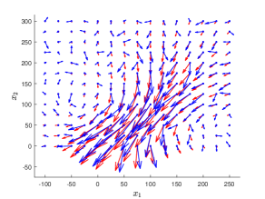
Figure 4: Plots of the data for solving the fault inverse problem in our simulations. The data are realizations of noisy horizontal surface displacements (blue) at the measurement points obtained by using the slip field shown in Figure 3 occurring on the fault $\Gamma$ shown in Figure 2. Top: low noise scenario. Bottom: high noise scenario. In each graph the unperturbed field is sketched in red.

3.2 Numerical results from our parallel sampling algorithm

The parallel sampling algorithm introduced in section 2.4 requires the knowledge of a prior distribution for the random variable $({\itbf m},\alpha)$. Here, we assume that the priors of ${\itbf m}$ and $\alpha$ are independent. The prior of ${\itbf m}$ is chosen to be uniformly distributed on the subset ${\cal B}$ of $[-200,200]^{6}$ such that the angle $\theta$ between the vectors normal to the two quadrilaterals whose union is $\Gamma$ satisfies $\cos\theta\geq 0.8$. That way, the angle between these two quadrilaterals is between 143 and 217 degrees: this can be interpreted as a regularity condition on the slip field ${\itbf g}$ since it was set to point in the direction of steepest descent. As to $\alpha$, we assumed that $\log_{10}\alpha$ follows a uniform prior on $[-5,0]$.
Next, we present results obtained by applying our parallel sampling algorithm to the data shown in Figure 4 for the low noise and the high noise scenario. Computations were performed on a parallel platform that uses $N_{par}=20$ processors. After computing the expected value of ${\itbf m}$, we sketched the corresponding geometry of $\Gamma$ (Figure 5, first row) by plotting depth contour lines. On the same graph we plotted the magnitude of the reconstructed slip field on $\Gamma$ as a function of $(x_{1},x_{2})$. This reconstruction was done by using the expected value of $({\itbf m},\alpha)$ and solving the linear system $(A_{\itbf m}^{\prime}A_{\itbf m}+\alpha R^{\prime}R){\itbf g}_{min}=A_{\itbf m}^{\prime}{\itbf u}$. The reconstructed slip field is very close to the true one shown in Figure 3. In the second row of Figure 5, we show the absolute value of the difference between the computed expected depth $x_{3}$ on $\Gamma$ minus its true value and a contour profile of the reconstructed slip ${\itbf g}_{min}$. It is noticeable that the error in reconstructing the depth in the high noise scenario is rather lower where ${\itbf g}_{min}$ is larger: this is in line with previous theoretical studies [20, 21] where it was proved that fault geometries can only be reconstructed on the support of slip fields. In the third row of Figure 5, we show two standard deviations for the reconstructed depth as a function of $(x_{1},x_{2})$, with again contour lines of ${\itbf g}_{min}$. We note that this difference (close to 2) is very low in the low noise scenario compared to the depth at the center of the support of ${\itbf g}_{min}$ (close to -40). In the high noise scenario the standard deviation is rather lower in the region where $|{\itbf g}_{min}|$ is larger. We show in Figure 6 reconstructed posterior marginal distribution functions for the six components of ${\itbf m}$ and for $\alpha$. Interestingly, we notice that the range of high probability for $\alpha$ is much higher in the higher noise scenario (more than 10 times higher, since the graph is that of $\log_{10}\alpha$). Intuitively, it is clear that stronger noise would require more regularization, as Morozov principle dictates [18], but the strength of our algorithm is that it automatically selects a good range for $\alpha$ without user input or prior knowledge about $\sigma$. In the low noise scenario, for all six components of ${\itbf m}$, the reconstructed posterior marginal distribution functions peak very close to their true value, the difference would not actually be visible on the graphs. The picture is quite different in the high noise scenario. The support of the distribution functions are much wider in that case and two peaks are apparent for $m_{1}$ and for $m_{2}$. The large width for these distribution functions is related to a much larger number of samples in the random walk for the algorithm to converge as illustrated in Figure 7. As to choosing a starting point $({\itbf m}_{1},\alpha_{1})$, we found that it was most efficient to draw $N_{burn}\times N_{par}$ samples from the prior and use these samples to compute an expected value, which we set to be equal to $({\itbf m}_{1},\alpha_{1})$.
To conclude this section, we would like to emphasize that the numerical results that we show in this paper are not so sensitive to the the particular realizations of the noise and the intrinsic randomness of Markov chains. We conducted a large number of simulations each starting from a different realization of ${\itbf u}$. In the low noise scenario, the differences between estimates of expected values and covariances were negligible. In the high noise scenario, the differences between estimates of expected values and covariances were more appreciable, however the difference between the expected value of the depth of $\Gamma$ and its true value as in row 2 of Figure 5, and the plot for the standard deviation of reconstructed depth as in row 3 of Figure 5, were comparable and the differences were small in the region of high values of the reconstructed slip ${\itbf g}_{min}$.

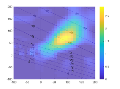
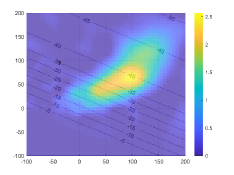
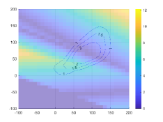
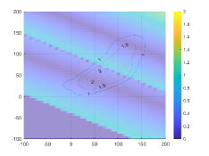
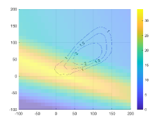
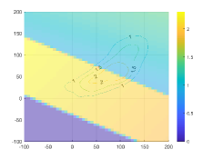
Figure 5: Reconstructed slip field ${\cal G}$ (discretized by ${\itbf g}_{min}$) and computed expected depth profile for the fault $\Gamma$ reconstructed from the data shown in Figure 4. In all six graphs in this figure, the horizontal axis is for $x_{1}$, and the vertical axis is for $x_{2}$. Left column: high noise scenario. Right column: low noise scenario. First row: depth contour lines for $\Gamma$ corresponding to the expected value of ${\itbf m}$ and the slip field modulus (shown in color) given that geometry and the computed expected value of $\alpha$. The slip field was obtained by applying the formula ${\itbf g}_{min}=(A_{\itbf m}^{\prime}A_{\itbf m}+\alpha R^{\prime}R)^{-1}A_{\itbf m}^{\prime}{\itbf u}$. Second row: absolute value of the difference between computed expected depth of $\Gamma$ and true depth as a function of $(x_{1},x_{2})$ shown in color, with contour lines of reconstructed $|{\cal G}|$. The third row shows two standard deviations for the reconstructed depth as a function of $(x_{1},x_{2})$, with again contour lines of reconstructed $|{\cal G}|$.

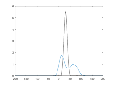
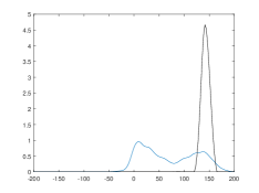
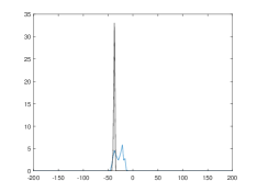
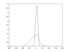
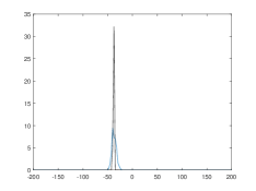
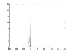
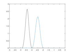
Figure 6: Reconstructed posterior marginal distribution functions for the six components of ${\itbf m}$ and for $\log_{10}\alpha$. Blue: high noise scenario. Black: low noise scenario. For ${\itbf m}$, true values are nearly indistinguishable from the peak of the black curves.

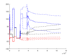
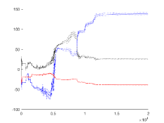
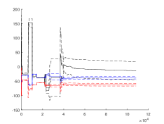
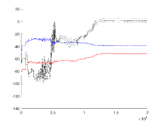
Figure 7: First row: evolution of computed expected values of $m_{1},m_{2},m_{3}$ (black, blue, and red solid lines) and one standard deviation envelopes. Left: high noise scenario. Right: low noise scenario. Second row: evolution of computed expected values of $m_{4},m_{5},m_{6}$ (black, blue, and red solid lines) and one standard deviation envelopes. Left: high noise scenario. Right: low noise scenario.

3.3 Comparison to methods based on GCV, ML, and CLS

For the GCV method, we minimized

$$\frac{\|(I_{n}-A_{\itbf m}(A_{\itbf m}^{\prime}A_{\itbf m}+\alpha R^{\prime}R)^{-1}A_{\itbf m}^{\prime}){\itbf u}\|^{2}}{\mbox{tr }(I_{n}-A_{\itbf m}(A_{\itbf m}^{\prime}A_{\itbf m}+\alpha R^{\prime}R)^{-1}A_{\itbf m}^{\prime})^{2}},$$

and for the ML method,

$$\frac{{\itbf u}^{\prime}(I_{n}-A_{\itbf m}(A_{\itbf m}^{\prime}A_{\itbf m}+\alpha R^{\prime}R)^{-1}A_{\itbf m}^{\prime}){\itbf u}}{(\det(I_{n}-A_{\itbf m}(A_{\itbf m}^{\prime}A_{\itbf m}+\alpha R^{\prime}R)^{-1}A_{\itbf m}^{\prime}))^{1/n}},$$

as functions in $({\itbf m},\alpha)$ where ${\itbf m}$ is in the subset ${\cal B}$ of $[-200,200]^{6}$ defined earlier and $\log_{10}\alpha$ is between -5 and 0. We used the Matlab 2020 function surrogateopt to search for the minimum. This function is based on a minimization algorithm proposed in [8] which is specifically designed for problems where function evaluations are expensive. This algorithm uses a radial basis function interpolation to determine the next point where the objective function should be evaluated. This is a global non-convex minimization algorithm that uses random restart points in an attempt to avoid being trapped in local minima. We report the computed minima for the high noise scenario in Figure 8, top left graph, where we also indicate the true value of ${\itbf m}$ and the computed expected value of ${\itbf m}$ obtained by our parallel sampling algorithm, together with the one standard deviation envelope. We observe that the computed values of ${\itbf m}$ obtained by the GCV or the ML algorithm are not as close to the true value of ${\itbf m}$ as the computed expected value of ${\itbf m}$. In this high noise scenario, the one standard deviation is particularly informative but it cannot be provided by the GCV or the ML algorithm. In the second graph of Figure 8, we show computed values of ${\itbf m}$ if the GCV and the ML algorithms are started from the particularly favorable point $\tilde{{\itbf m}}=(0,100,-20,0,-20,-30)$ and $\tilde{\alpha}=10^{-4}$. These two algorithms perform only marginally better despite this favorable head start. In Figure 9, we report results for the low noise scenario. It is even clearer in that case that our parallel sampling algorithm outperforms the GCV and the ML methods even if they are provided with the favorable starting point $\tilde{{\itbf m}}$.
We also show results obtained by the CLS method in the third graph of Figure 8 for the high noise scenario, Figure 9 for the low noise scenario. In our particular application $\sigma$ is not known, and even then it would be unclear what fixed value to choose for $\alpha$ because of the problem dependence on ${\itbf m}$. It is then common to try fixing a few values for $\alpha$ (we show results for four values of $\alpha$), and to minimize $\|A_{\itbf m}{\itbf g}-{\itbf u}\|^{2}+\alpha\|R{\itbf g}\|^{2}$ in ${\itbf m}$ and ${\itbf g}$. In the high noise scenario, if $\alpha=10^{-4}$, this led to results that are better than those obtained by the GCV or the ML methods. In the low noise scenario, best results were obtained for $\alpha=10^{-3}$, beating again GCV and ML. The caveat is that in a real world situation, the solution to the inverse problem is unknown, so it would be difficult to decide which of the four CLS solutions to select.

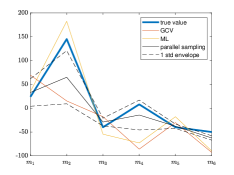
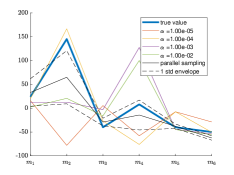
Figure 8: Computed values of ${\itbf m}$ for the high noise scenario. Top left: results obtained by the GCV and the ML methods without providing a starting point. Top right: values obtained if these methods are started from the favorable point $\tilde{{\itbf m}}$. Bottom: the CLS method for different values of $\alpha$ and resulting computed ${\itbf m}$. In each graph, the true value of ${\itbf m}$ and the expected value of ${\itbf m}$ with the one standard deviation envelope computed by the parallel sampling method introduced in this paper are indicated for comparison.

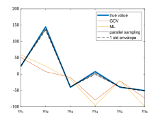
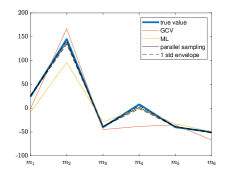
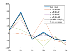
Figure 9: Same caption as in Figure 8 for the low noise scenario.

4 Conclusion and perspectives for future work

We have proposed in this paper an algorithm for a finite dimensional inverse problem that combines a linear unknown ${\itbf g}$ and a nonlinear unknown ${\itbf m}$. We have used the maximum likelihood assumption for the prior of ${\itbf g}$ scaled by a parameter $\alpha$ to derive a posterior distribution for $({\itbf m},\alpha)$. Using this posterior distribution we have built a parallel sampling algorithm for computing the expected value, the covariance, and the marginal probability distributions of ${\itbf m}$. This algorithm is particularly well suited to the fault inverse problem where ${\itbf m}$ models a set of geometry parameters for the fault and ${\itbf g}$ models a slip on that fault, while the data ${\itbf u}$ is sparse and noisy and the linear operator giving ${\itbf u}$ from ${\itbf g}$ has an unbounded inverse. Our numerical simulations have shown that our parallel sampling algorithm leads to better results than those obtained from minimizing the ML, the GCV, or the CLS functionals. Our algorithm automatically adjusts to a good range for the regularization parameter $\alpha$ relative to the noise level and avoids being trapped in local minima.
So far, our numerical simulations have focused on the case $q<<n<<p$, where ${\itbf m}$ is in $\mathbb{R}^{q}$, the measurements ${\itbf u}$ are in $\mathbb{R}^{n}$, and the forcing term ${\itbf g}$ is in $\mathbb{R}^{p}$. However, there are applications in geophysical sciences where measurements are nearly continuous in space and time. This often comes at the price of higher error margins, so this would correspond to the case where $n$ and $p$ are of the same order of magnitude, but $\sigma$ is larger, where $\sigma^{2}I_{n}$ is the covariance of the noise. Another interesting line of research would be to consider the case where $q$ is much larger which would model an inverse problem that depends non-linearly on a function, for example the coefficient of a PDE.

Funding
This work was supported by Simons Foundation Collaboration Grant [351025].

Appendix A Proof of formula (2.6)

It is well known that the non-zero eigenvalues of $A_{\itbf m}^{\prime}A_{\itbf m}$ and $A_{\itbf m}A_{\itbf m}^{\prime}$ are the same thus

$$\det(\alpha^{-1}A_{\itbf m}^{\prime}A_{\itbf m}+I_{p})=\det(\alpha^{-1}A_{\itbf m}A_{\itbf m}^{\prime}+I_{n}).$$

Expanding and simplifying shows that

$$(I_{n}-A_{\itbf m}(\alpha I_{p}+A_{\itbf m}^{\prime}A_{\itbf m})^{-1}A_{\itbf m}^{\prime})(I_{n}+\alpha^{-1}A_{\itbf m}A_{\itbf m}^{\prime})=I_{n},$$

thus,

$$(I_{n}+\alpha^{-1}A_{\itbf m}A_{\itbf m}^{\prime})^{-1}=I_{n}-A_{\itbf m}(\alpha I_{p}+A_{\itbf m}^{\prime}A_{\itbf m})^{-1}A_{\itbf m}^{\prime},$$

and formula (2.6) is now clear.

References

- [1] A. Aspri, E. Beretta, and A. L. Mazzucato. Dislocations in a layered elastic medium with applications to fault detection. preprint arXiv:2004.00321v1, 2020.
- [2] A. Aspri, E. Beretta, A. L. Mazzucato, and V. Maarten. Analysis of a model of elastic dislocations in geophysics. Archive for Rational Mechanics and Analysis, 236(1):71–111, 2020.
- [3] C. M. Bishop et al. Neural networks for pattern recognition. Oxford university press, 1995.
- [4] B. Calderhead. A general construction for parallelizing metropolis- hastings algorithms. Proceedings of the National Academy of Sciences, 111(49):17408–17413, 2014.
- [5] N. P. Galatsanos and A. K. Katsaggelos. Methods for choosing the regularization parameter and estimating the noise variance in image restoration and their relation. IEEE Transactions on image processing, 1(3):322–336, 1992.
- [6] G. Golub and V. Pereyra. Separable nonlinear least squares: the variable projection method and its applications. Inverse problems, 19(2):R1, 2003.
- [7] G. H. Golub, M. Heath, and G. Wahba. Generalized cross-validation as a method for choosing a good ridge parameter. Technometrics, 21(2):215–223, 1979.
- [8] H.-M. Gutmann. A radial basis function method for global optimization. Journal of global optimization, 19(3):201–227, 2001.
- [9] P. Jacob, C. P. Robert, and M. H. Smith. Using parallel computation to improve independent metropolis–hastings based estimation. Journal of Computational and Graphical Statistics, 20(3):616–635, 2011.
- [10] G. Little and J. Reade. Eigenvalues of analytic kernels. SIAM journal on mathematical analysis, 15(1):133–136, 1984.
- [11] V. A. Morozov. On the solution of functional equations by the method of regularization. In Doklady Akademii Nauk, volume 167, pages 510–512. Russian Academy of Sciences, 1966.
- [12] Y. Okada. Internal deformation due to shear and tensile faults in a half-space. Bulletin of the Seismological Society of America, vol. 82 no. 2:1018–1040, 1992.
- [13] G. O. Roberts and J. S. Rosenthal. Examples of adaptive mcmc. Journal of Computational and Graphical Statistics, 18(2):349–367, 2009.
- [14] G. O. Roberts, J. S. Rosenthal, et al. Optimal scaling for various metropolis-hastings algorithms. Statistical science, 16(4):351–367, 2001.
- [15] A. M. Stuart. Inverse problems: a bayesian perspective. Acta numerica, 19:451, 2010.
- [16] A. Thompson, J. Kay, and D. Titterington. A cautionary note about crossvalidatory choice. Journal of Statistical Computation and Simulation, 33(4):199–216, 1989.
- [17] J. M. Varah. Pitfalls in the numerical solution of linear ill-posed problems. SIAM Journal on Scientific and Statistical Computing, 4(2):164–176, 1983.
- [18] C. R. Vogel. Computational methods for inverse problems, volume 23. Siam, 2002.
- [19] D. Volkov. A double layer surface traction free green’s tensor. SIAM Journal on Applied Mathematics, 69(5):1438–1456, 2009.
- [20] D. Volkov and J. C. Sandiumenge. A stochastic approach to reconstruction of faults in elastic half space. Inverse Problems & Imaging, 13(3):479–511, 2019.
- [21] D. Volkov, C. Voisin, and I. Ionescu. Reconstruction of faults in elastic half space from surface measurements. Inverse Problems, 33(5), 2017.
- [22] D. Volkov, C. Voisin, and I. I.R. Determining fault geometries from surface displacements. Pure and Applied Geophysics, 174(4):1659–1678, 2017.