Improving Adversarial Robustness by Enforcing Local and Global Compactness

Abstract

The fact that deep neural networks are susceptible to crafted perturbations severely impacts the use of deep learning in certain domains of application. Among many developed defense models against such attacks, adversarial training emerges as the most successful method that consistently resists a wide range of attacks. In this work, based on an observation from a previous study that the representations of a clean data example and its adversarial examples become more divergent in higher layers of a deep neural net, we propose the Adversary Divergence Reduction Network which enforces local/global compactness and the clustering assumption over an intermediate layer of a deep neural network. We conduct comprehensive experiments to understand the isolating behavior of each component (i.e., local/global compactness and the clustering assumption) and compare our proposed model with state-of-the-art adversarial training methods. The experimental results demonstrate that augmenting adversarial training with our proposed components can further improve the robustness of the network, leading to higher unperturbed and adversarial predictive performances.

1 Introduction

Despite the great success of deep neural nets, they are reported to be susceptible to crafted perturbations [27, 7], even state-of-the-art ones. Accordingly, many defense models have been developed, notably [19, 29, 28, 22]. Recently, the work of [1] undertakes an in-depth study of neural network defense models and conduct comprehensive experiments on a complete suite of defense techniques, which has lead to postulating one common reason why many defenses provide apparent robustness against gradient-based attacks, namely obfuscated gradients.

According to the above study, adversarial training with Projected Gradient Descent (PGD) [19] is one of the most successful and widely-used defense techniques that remained consistently resilient against attacks, which has inspired many recent advances including Adversarial Logit Pairing (ALP) [12], Feature Denoising [28], Defensive Quantization [17], Jacobian Regularization [10], Stochastic Activation Pruning [5], and Adversarial Training Free [24].

In this paper, we propose to build robust classifiers against adversarial examples by learning better representations in the intermediate space. Given an image classifier based on a multi-layer neural net, conceptually, we divide the network into two parts with an intermediate layer: the generator network from the input layer to the intermediate layer and the classifier network from the intermediate layer to the output prediction layer. The output of the generator network (i.e., the intermediate layer) is the intermediate representation of the input image, which is fed to the classifier network to make prediction. For image classifiers, an adversarial example is usually generated by adding small perturbations to a clean image. The adversarial example may look very similar to the original image but leads to significant changes to the prediction of the classifier. It has been observed that in deep neural networks, the representations of a clean data example and its adversarial example might become very diverge in the intermediate space, although their representations are proximal in the data space [28]. Due to the above divergence in the intermediate space, a classifier may be hard to predict the same class of the adversarial and real images. Inspired by this observation, we propose to learn better representations that reduce the above divergence in the intermediate space, so as to enhance the classifier robustness against adversarial examples.

In particular, we propose an enhanced adversarial training framework that imposes the local and global compactness properties on the intermediate representations, to build more robust classifiers against adversarial examples. Specifically, by explicitly strengthening local compactness, we enforce the intermediate representations output from the generator of a clean image and its adversarial examples to be as proximal as possible. In this way, the classifier network is less easy to be misled by the adversarial examples. However, enforcing the local compactness itself may not be sufficient to guarantee a robust defense model as the representations might be encouraged to globally spread out in the intermediate space, significantly hurting accuracies on both clean and adversarial images. To address this, we further propose to impose global compactness to encourage the representations of examples in the same class to be proximal yet those in different classes to be more distant. Finally, to increase the generalization capacity of the deep network and reduce the misclassification of adversarial examples, our framework enjoys the flexibility to incorporate the clustering assumption [3], which aims to force the decision boundary of a classifier to lie in the gap between clusters of different classes. By collaboratively incorporating the above three properties, we are able to learn better intermediate representations, which help to boost the adversarial robustness of classifiers. Intuitively, we name our proposed framework to the Adversary Divergence Reduction Network (ADR).

To comprehensively exam the proposed framework, we conduct extensive experiments to investigate the influence of each component (i.e., local/global compactness and the clustering assumption), visualize the smoothness of the loss surface of our robust model, and compare our proposed ADR method with several state-of-the-art adversarial defenses. The experimental results consistently show that our proposed method can further improve over others in terms of better adversarial and clean predictive performances. The contributions of this work are summarized as follows:

• We propose the local and global compactness properties on the intermediate space to enforce the better representations, which lead to more robust classifiers;

• We incorporate our local and global compactness with clustering assumption to further enhance adversarial robustness;

• We plug the above three components into an adversarial training framework to introduce our Adversary Divergence Reduction Network;

• We extensively analyze the proposed framework and compare it with state-of-the-art adversarial training methods to verify its effectiveness.

2 Related works

2.0.1 Adversarial training defense

Adversarial training can be traced back to [7], in which models were challenged by producing adversarial examples and incorporating them into training data. The adversarial examples could be the worst-case examples (i.e., $x_{a}\triangleq\text{argmax}{}_{x^{\prime}\in B_{\varepsilon}\left(x\right)}\ell\left(x^{\prime},y,\theta\right)$) [7] or most divergent examples (i.e., $x_{a}\triangleq\text{argmax}{}_{x^{\prime}\in B_{\varepsilon}\left(x\right)}D_{KL}\left(h_{\theta}\left(x^{\prime}\right)\mid\mid h_{\theta}\left(x\right)\right)$) [29] where $D_{KL}$ is the Kullback-Leibler divergence and $h_{\theta}$ is the current model. The quality of the adversarial training defense crucially depends on the strength of the injected adversarial examples – e.g., training on non-iterative adversarial examples obtained from FGSM or Rand FGSM (a variant of FGSM where the initial point is randomised) are not robust to iterative attacks, for example PGD [19] or BIM [15].

Although many defense models were broken by [1], the adversarial training with PGD [19] was among the few that were resilient against attacks. Many defense models were developed based on adversarial examples from a PGD attack or attempts made to improve and scale up the PGD adversarial training. Notable examples include Adversarial Logit Pairing (ALP) [12], Feature Denoising [28], Defensive Quantization [17], Jacobian Regularization [10], Stochastic Activation Pruning [5], and Adversarial Training for Free [24].

2.0.2 Defense with a latent space

These works utilized a latent space to enable adversarial defense, notably [11]. DefenseGAN [23] and PixelDefense [26] use a generator (i.e., a pretrained WS-GAN [8] for DefenseGAN and a PixelCNN [21] for PixelDefense) together with the latent space to find a denoised version of an adversarial example on the data manifold. These works were criticized by [1] as being easy to attack and impossible to work within the case of the CIFAR-10 dataset. Jalal et al. [11] proposed an overpowered attack method to efficiently attack both DefenseGAN and PixelDefense and subsequently injected those adversarial examples to train the model. Though that work was proven to work well with simple datasets including MNIST and CelebA, no experiments were conducted on more complex datasets including, for example, CIFAR-10.

3 Proposed method

In what follows, we present our proposed method, named the Adversary Divergence Reduction Network (ADR). As shown in the previous study [28], although an adversarial example $x_{a}$ and its corresponding clean example $x$ are in close proximity in the data space (i.e., differ by a small perturbation), when brought forward up to the higher layers in a deep neural network, their representations become markedly more divergent, hence causing different prediction results. Inspired by this observation, we propose imposing local compactness for those representations in an intermediate layer of a neural network. The key idea is to enforce that the representations of an adversarial example and its clean counterpart be as proximal as possible, hence reducing the chance of misclassifying them. Moreover, we observe that enforcing the local compactness itself is not sufficient to guarantee a robust defense model as this enforcement might encourage representations to globally spread out across the intermediate space (i.e., the space induced by the intermediate representations), significantly hurting both adversarial and clean performances. To address this, we propose to impose global compactness for the intermediate representations such that representations of examples that belong in the same class are proximal and those in different classes are more distant. Finally, to increase the generalization capacity of the deep network and reduce the misclassification of adversarial examples, we propose to apply the clustering assumption [3] which aims to force the decision boundary to lie in the gap between clusters of different classes, hence increasing the chance for adversarial examples to be correctly classified.

3.1 Local compactness

Local compactness, which aims to reduce the divergence between the representations of an adversarial example and its clean example in an intermediate layer, is one of the key aspects of our proposed method. Let us denote our deep neural network by $h_{\theta}\left(\cdot\right)$, which decomposes into $h_{\theta}\left(\cdot\right)=g_{\theta}\left(f_{\theta}\left(\cdot\right)\right)$ where the first (generator) network $f_{\theta}$ maps the data examples onto an intermediate layer where we enforce the compactness constraints. The following (classifier) network $g_{\theta}$ maps the intermediate representations to the prediction output. For local compactness, given a clean data example $x$, denote $\mathcal{A}_{\varepsilon}$ as a stochastic adversary that renders adversarial examples for $x$ as $x_{a}\sim\mathcal{A}_{\varepsilon}\left(x\right)$ in a ball $B_{\varepsilon}\left(x\right)=\left\{x^{\prime}:\left\|x-x^{\prime}\right\|<\varepsilon\right\}$, our aim is to compress the representations of $x$ and $x_{a}$ in the intermediate layer by minimizing

$$\mathcal{{L}}_{\text{com}}^{\text{lc}}=\mathbb{{E}}_{x\sim\mathcal{D}_{x}}\left[\mathbb{{E}}_{x_{a}\sim\mathcal{A}_{\varepsilon}\left(x\right)}\left[\left\|f_{\theta}(x)-f_{\theta}(x_{a})\right\|_{p}\right]\right]$$ (1)

where we use $\mathcal{D}_{x}=\left\{x_{1},...,x_{N}\right\}$ to represent both training examples and the corresponding empirical distribution and $\left\|\cdot\right\|_{p}$ with $p=1,2,\infty$ to specify the $p$-norm.

3.2 Global compactness

For global compactness, we want the representations of data examples in the same class to be closer and data examples in different classes to be more separate. As demonstrated later, global compactness in conjunction with the clustering assumption helps increase the margin of a data example (i.e., the distance from that data example to the decision boundary), hence boosting the generalization capacity of the classifier network and adversarial robustness.

More specifically, given two examples $\left(x_{i},y_{i}\right)$ and $\left(x_{j},y_{j}\right)$ drawn from the empirical distribution over $\mathcal{D}_{x,y}=\left\{\left(x_{1},y_{1}\right),...,\left(x_{N},y_{N}\right)\right\}$ where the label $y_{k}\in\left\{1,2,...,M\right\}$, we compute the weight $w_{ij}$ for this pair as follows:

$$w_{ij}=\frac{\alpha-\mathbb{I}_{y_{i}\neq y_{j}}}{\alpha}=\begin{cases}1&\text{if}\,y_{i}=y_{j}\\ \frac{\alpha-1}{\alpha}&\text{otherwise}\end{cases}$$ (2)

where $\mathbb{I}_{S}$ is the indicator function which returns 1 if $S$ holds and $0$ otherwise. We consider $\alpha\in(0,1)$, yielding $w_{ij}<0$ if $y_{i}\neq y_{j}$ and $w_{ij}>0$ if otherwise.

We enforce global compactness by minimizing

$$\mathcal{{L}}_{\text{com}}^{\text{gb}}=\mathbb{{E}}_{\left(x_{i},y_{i}\right),\left(x_{j},y_{j}\right)\sim\mathcal{D}_{x,y}}\left[w_{ij}\left\|f_{\theta}(x_{i})-f_{\theta}(x_{j})\right\|_{p}\right]$$ (3)

where we overload the notation $\mathcal{D}_{x,y}$ to represent the empirical distribution over the training set, which implies that the intermediate representations $f_{\theta}(x_{i})\text{ }$ and $f_{\theta}(x_{j})$ are encouraged to be closer if $y_{i}=y_{j}$ and to be separate if $y_{i}\neq y_{j}$ for a global compact representation.

Note that in our experiment, we set $\alpha=0.99$, yielding $w_{ij}\in\{1,-0.01\}$, and calculate global compactness with each random minibatch.

3.3 Clustering assumption and label supervision

At this stage, we have achieved compact intermediate representations for the clean data and adversarial examples obtained from a stochastic adversary $\mathcal{A}_{\varepsilon}$. Our next step is to enforce some constraints on the subsequent classifier network $g_{\theta}$ to further exploit this compact representation for improving adversarial robustness. The first constraint we impose on the classifier network $g_{\theta}$ is that this should classify both clean data and adversarial examples correctly by minimizing

$$\mathcal{L}_{\text{c}}=\mathbb{E}_{\left(x,y\right)\sim D_{x,y}}\Biggl{[}\mathbb{E}_{x_{a}\sim\mathcal{A}_{\varepsilon}\left(x\right)}\left[\ell\left(h_{\theta}\left(x_{a}\right),y\right)\right]+\ell\left(h_{\theta}\left(x\right),y\right)\Biggr{]}$$ (4)

where $\ell$ is the cross-entropy loss function.

In addition to this label supervision, the second constraint we impose on the classifier network $g_{\theta}$ is the clustering assumption [3], which states that the decision boundary of $g_{\theta}$ in the intermediate space should not break into any high density region (or cluster) of data representations in the intermediate space, forcing the boundary to lie in gaps formed by those clusters. The clustering assumption when combined with the global compact representation property should increase the data example margin (i.e., the distance from that data example to the decision boundary). If this is further combined with the fact that the representations of adversarial examples are compressed into the representation of its clean data example (i.e. local compactness) this should also reduce the chance that adversarial examples are misclassified. To enforce the clustering assumption, inspired by [25], we encourage the classifier confidence by minimizing the conditional entropy and maintain classifier smoothness using Virtual Adversarial Training (VAT) [20], respectively:

$$\mathcal{{L}}_{\text{conf}}=\mathbb{{E}}_{x\sim D_{x}}\Biggl{[}\mathbb{{E}}_{x_{a}\sim\mathcal{A}_{\varepsilon}\left(x\right)}\left[-h_{\theta}(x_{a})^{T}\log h_{\theta}(x_{a})\right]-h_{\theta}(x)^{T}\log h_{\theta}(x)\Biggr{]}$$ (5)

$$\mathcal{{L}}_{\text{smt}}=\mathbb{{E}}_{x\sim D_{x}}\left[\mathbb{{E}}_{x_{a}\sim\mathcal{A}_{\varepsilon}\left(x\right)}\left[D_{KL}\left(h_{\theta}(x)\|h_{\theta}(x_{a})\right)\right]\right]$$ (6)

3.4 Generating adversarial examples

We can use any adversarial attack algorithm to define the adversary $\mathcal{A}_{\varepsilon}$. For example, Madry et al. [19] proposed to find the worst-case examples $x_{a}\triangleq\text{argmax}{}_{x^{\prime}\in B_{\varepsilon}\left(x\right)}\ell\left(x^{\prime},y,\theta\right)$ using PGD, while Zhang et al. [29] aimed to find the most divergent examples $x_{a}\triangleq\text{argmax}{}_{x^{\prime}\in B_{\varepsilon}\left(x\right)}D_{KL}\left(h_{\theta}\left(x^{\prime}\right)\mid\mid h_{\theta}\left(x\right)\right).$ By enforcing local/global compactness over the adversarial examples obtained by $\mathcal{A}_{\varepsilon}$, we make them easier to be trained with the label supervision loss in Eq. (4), hence eventually improving adversarial robustness. The quality of adversarial examples obviously affects to the overall performance, however, in the experimental section, we empirically prove that our proposed components can boost the robustness of the adversarial training frameworks of interest.

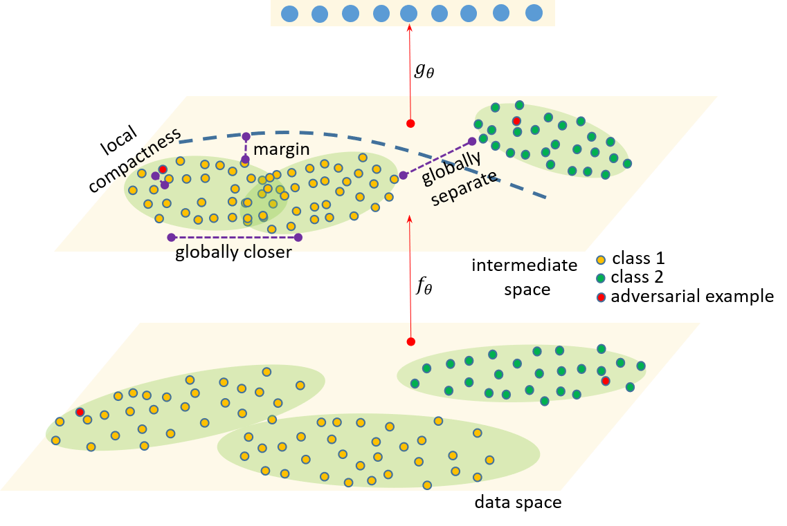
Figure 1: Overview of Adversary Divergence Reduction Network. The local/global compactness and clustering assumption are intended to improve adversarial robustness.

3.5 Putting it all together

We combine the relevant terms regarding local/global compactness, label supervision, and the clustering assumption and arrive at the following optimization problem:

$$\min_{\theta}\,\mathcal{L}\triangleq\mathcal{L}_{\text{c}}+\lambda_{\text{com}}^{\text{lc}}\mathcal{L}_{\text{com}}^{\text{lc}}+\lambda_{\text{com}}^{\text{gb}}\mathcal{L}_{\text{com}}^{\text{gb}}+\lambda_{\text{conf}}\mathcal{L}_{\text{conf}}+\lambda_{\text{smt}}\mathcal{L}_{\text{smt}}$$ (7)

where $\lambda_{\text{com}}^{\text{lc}},\lambda_{\text{com}}^{\text{gb}},\lambda_{\text{conf}},\text{ and }\lambda_{\text{smt}}$ are non-negative trade-off parameters.

In Figure 1, we illustrate how the three components, namely local/global compactness, label supervision, and the clustering assumption can mutually collaborate to improve adversarial robustness. The representations of data examples via the network $f_{\theta}$ are enforced to be locally/globally compact, whereas the position of the decision boundary of the classifier network $g_{\theta}$ in the intermediate space is enforced using the clustering assumption. Ideally, with the clustering assumption, the decision boundary of $g_{\theta}$ preserves the cluster structure in the intermediate space and when combined with label supervision training ensures clusters in a class remain completely inside the decision region for this class. Moreover, global compactness encourages clusters of a class to be closer and those of different classes to be more separate. As a result, the decision boundary of $g_{\theta}$ lies in the gaps among clusters as well as with a sufficiently large margin for the data examples. Finally, local compactness requires adversarial examples to stay closer to their corresponding clean data example, hence reducing the chance of misclassifying them and therefore improving adversarial robustness.

Comparison with the contrastive learning.

Interestingly, the contrastive learning [4, 9] and our proposed method aim to learn better representations by the principle of enforcing similar elements to be equal and dissimilar elements to be different. However, the contrastive learning works on an instance level, which enforces the representation of an image to be proximal with those of its transformations and to be distant with those of any other images. On the other hand, our method works on a class level, which enforces the intermediate representations of each class to be compact and well separated with those in other classes. Therefore, our method and the contrastive learning complement each other and intuitively improve both visual representation and adversarial robustness when combining together.

4 Experiments

In this section, we first introduce the general setting for our experiments regarding datasets, model architecture, optimization scheduler, and adversary attackers. Second, we compare our method with adversarial training with PGD, namely ADV [19] and TRADES [29]. We employ either ADV or TRADES as the stochastic adversary $\mathcal{A}$ for our ADR and demonstrate that, when enhanced with local/global compactness and the clustering assumption, we can improve these state-of-the-art adversarial training methods.

Specifically, we begin this section with an ablation study to investigate the model behaviors and the influence of each component, namely local compactness, global compactness, and the clustering assumption, on adversarial performance. In addition, we visualize the smoothness of the loss surface of our model to understand why it can defend well. Finally, we undertake experiments on the MNIST and CIFAR-10 datasets to compare our ADR with both ADV and TRADES.

4.1 Experimental setting

General setting

We undertook experiments on both the MNIST [16] and CIFAR-10 [13] datasets. The inputs were normalized to $[0,1]$. For the CIFAR-10 dataset, we apply random crops and random flips as describe in [19] during training. For the MNIST dataset, we used the standard CNN architecture with three convolution layers and three fully connected layers described in [2]. For the CIFAR-10 dataset, we used two architectures in which one is the standard CNN architecture described in [2] and another is the ResNet architecture used in [19]. We note that there is a serious overfitting problem on the CIFAR-10 dataset as mentioned in [2]. In our setting, with the standard CNN architecture, we eventually obtained a $98\%$ training accuracy, but only a $75\%$ testing accuracy. With the ResNet architecture, we used the strategy from [19] to adjust the learning rate when training to reduce the gap between the training and validation accuracies. For the MNIST dataset, a drop-rate equal to 0.1 at epochs 55, 75, and 90 without weight decay was employed. For the CIFAR-10 dataset, the drop-rate was set to 0.1 at epochs 100 and 150 with weight decay equal to $2\times 10^{-4}$. We use a momentum-based SGD optimizer for the training of the standard CNN for the MNIST dataset and the ResNet for the CIFAR-10 dataset, while using the Adam optimizer for training the standard CNN on the CIFAR-10 one. The hyperparameters setting can be found in the supplementary material.

Choosing the intermediate layer.

The intermediate layer for enforcing compactness constraints immediately follows on from the last convolution layer for the standard CNN architecture and from the penultimate layer for the ResNet architecture. Moreover, we provide an additional ablation study to investigate the importance of choosing the intermediate layer which can be found in the supplementary material.

Attack methods

We use PGD to challenge the defense methods in this paper. Specifically, the setting for the MNIST dataset is PGD-40 (i.e., PGD with 40 steps) with the distortion bound $\varepsilon$ increasing from $0.1$ to $0.7$ and step size $\eta\in\{0.01,0.02\}$, while that for CIFAR-10 is PGD-20 with $\varepsilon$ increasing from $0.0039\,(\approx 1/255)$ to $0.11\,(\approx 28/255)$ and step size $\eta\in\{0.0039,0.007\}$. The distortion metric is $l_{\infty}$ for all attacks. For the adversarial training, we use $k=10$ for CIFAR10 and $k=20$ for MNIST for all defense methods.

Non-targeted and multi-targeted attack scenarios

We used two types of attack scenarios, namely non-targeted and multi-targeted attacks. The non-targeted attack derives adversarial examples by maximizing the loss w.r.t. its clean data label, whilst the multi-targeted attack is undertaken by performing simultaneously targeted attack for all possible data labels. The multi-targeted attack is considered to be successful if any individual targeted attack on each target label is successful. While the non-targeted attack considers only one direction of the gradient, the multi-targeted attack takes multi-directions of gradient into account, which guarantees to get better local optimum.

4.2 Experimental results

In this section, we first conduct an ablation study using the MNIST dataset in order to investigate how the different components (local compactness, global compactness, and the clustering assumption) contribute to adversarial robustness. We then conduct experiments on the MNIST and CIFAR-10 datasets to compare our proposed method with ADV and TRADES. Further evaluation can be found in the supplementary material.

4.2.1 Ablation study

We first study how each proposed component contributes to adversarial robustness. We use adversarial training with PGD as the baseline model and experiment on the MNIST dataset. Recall that our method consists of three components: the local compactness loss $\mathcal{L}_{\text{com}}^{\text{lc}}$, the global compactness loss $\mathcal{{L}}_{\text{com}}^{\text{gb}}$, and the clustering assumption loss which combines $\{\mathcal{{L}}_{\text{smt}}+\mathcal{{L}}_{\text{conf}}\}$ . In this experiment, we simply set the trade-off parameters $\lambda_{\text{com}}^{\text{lc}},\lambda_{\text{com}}^{\text{gb}},\lambda_{\text{smt}}=\lambda_{\text{conf}}=\lambda_{\text{ca}}$ to $0/1$ to deactivate/activate the corresponding component. We consider two metrics: the natural accuracy (i.e., the clean accuracy) and the robustness accuracy to evaluate a defense method. The natural accuracy is that evaluated on the clean test images, while the robustness accuracy is that evaluated on adversarial examples generated by attacking the clean test images. It is noteworthy that for many existing defense methods, improving robustness accuracy usually harms natural accuracy. Therefore, our proposed method aims to reach a better trade-off between the two metrics.

Table 1 shows the results for the PGD attack with $k=40,\,\varepsilon=0.325,\text{ and }\eta=0.01$. We note that ADR-None is our base model without any additional components. The base model can be any adversarial training based method, e.g., ADV or TRADES. Without loss of generality, we use ADV as the base model, i.e., ADR-None. By gradually combining the proposed additional components with ADR-None we produce several variants of ADR (e.g., ADR+LC is ADR-None together with the local compactness component). Since the standard model was trained without any defense mechanism, its natural accuracy is high at $99.5\%$ whereas the robustness accuracy is very poor at $0.88\%$, indicating its vulnerability to adversarial attacks. Regarding the variants of our proposed models, those with additional components generally achieve higher robustness accuracies compared with ADR-None (i.e. ADV), without hurting the natural accuracy. In addition, the robust accuracy was significantly improved with global compactness and the clustering assumption terms.

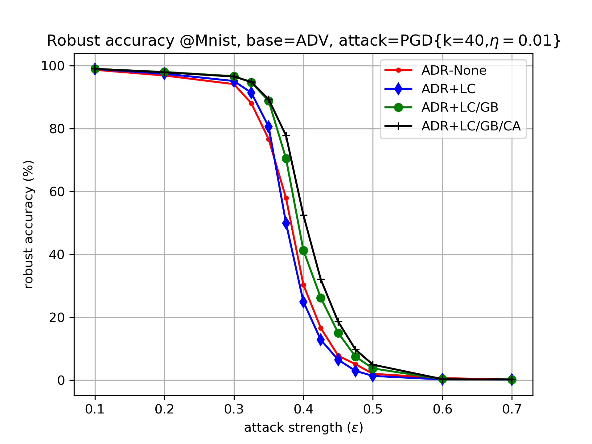
Figure 2: Variation of the robustness accuracies under different attack strengths. The base model is ADV (ADR-None).

Table 1: Results of the PGD-40 attack on the MNIST dataset for the base ADV model together with its variants with the different components (LC = local compactness, GB = global compactness, CA = clustering assumption) and $\varepsilon=0.325$.

	Nat. acc.	Rob. acc.
Standard model	99.5%	0.84%
ADR-None (ADV)	99.27%	88.1%
ADR+LC	99.41%	91.43%
ADR+LC/GB	99.35%	94.52%
ADR+LC/GB/CA	99.36%	94.96%

We also evaluate the metrics of interest with different attack strength by increasing the distortion boundary $\varepsilon$ as shown in Figure 2. By just adding a single local compactness component, our method can improve the base model (ADV or ADR-None) for attacks with strength $\varepsilon\leq 0.35$. By adding the global compactness component, our method can significantly improve over the base model, especially for stronger attacks. Recall that as we generate adversarial examples from the PGD attack with $k=20,\varepsilon_{d}=0.3,\eta=0.01$ to train the defense models, is is unsurprised to see a model defends well with $\varepsilon\leq 0.3$. Interestingly, by adding our components, our defense methods can also achieve reasonably good robustness accuracy of $80\%$, even when $\varepsilon$ varies from 0.34 to $0.37$, indicating the better generality of our methods.

To gain a better understanding of the contribution of the local compactness component, we visualize the loss surface of the base model (ADV as ADR-None) and the base model with only the local compactness term (ADR+LC). In Figure 3, the left image is a clean data example $x$, while the middle image is the loss surface over the input region around $x$ in which the z-axis indicates the cross-entropy loss w.r.t. the true label (the higher value means more incorrect prediction) and the x- and y-axis indicates the variance of the input image along the gradient direction w.r.t. $x$ and a random orthogonal direction, respectively. By varying along the two axes, we create a grid of images which represents the neighborhood region around $x$. The right-hand image depicts the predicted labels corresponding with this input grid.

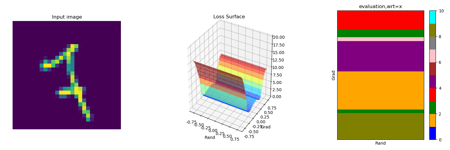
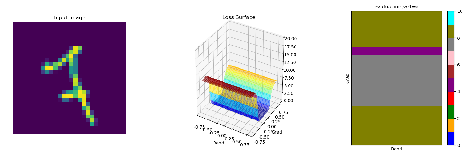
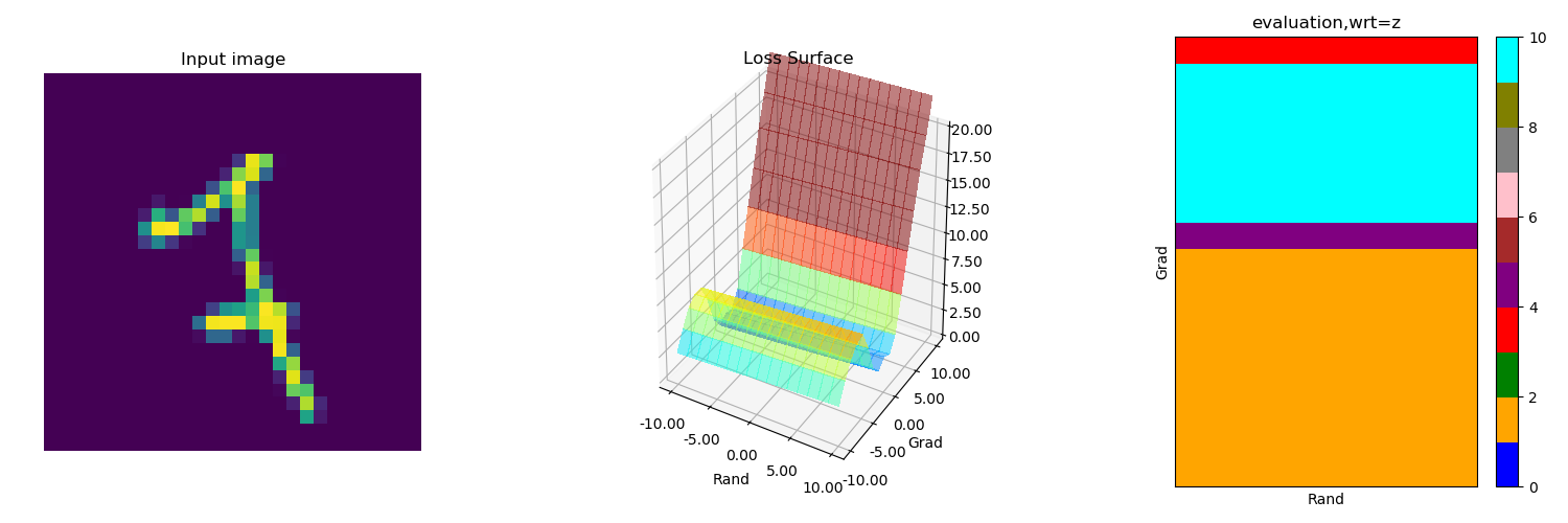
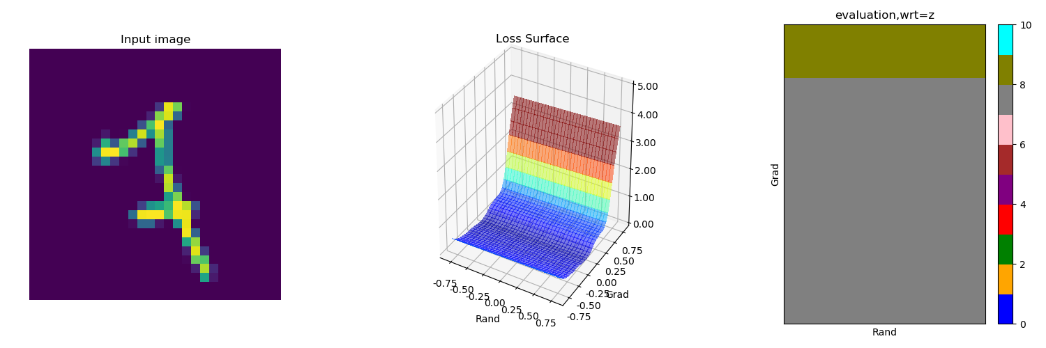
Figure 3: Loss surface at local region of a clean data example. Top-left: ADR-None w.r.t input. Top-right: ADR+LC w.r.t input. Bottom-left: ADR-None w.r.t latent. Bottom-right: ADR+LC w.r.t latent

From Figure 3, for ADR-None, that its neighborhood region is non-smooth, resulting in incorrect predictions to the label 1 and 4. Meanwhile, for our ADR+LC method (adversarial training with local compactness), the loss surface w.r.t. the input is smoother in its neighborhood region, resulting in correct predictions. In addition, in our method, the prediction surface w.r.t. the latent feature in the intermediate representation layer is smoother than that w.r.t. input. This means that our local compactness makes the local region more compact, hence improving adversarial robustness. Visualization with an adversarial example as input can be found in our supplementary material which provides more evidence of our improvement over the base model.

Furthermore, we use t-SNE [18] to visualize the intermediate space for demonstrating the effect of our global compactness component. We choose to show a positive adversarial example defined as an adversarial example which successfully fools a defense method. We compare the base model (ADV as ADR-None) with our method with the compactness terms and use t-SNE to project clean data and adversarial examples onto 2D space as in Figure 4. For ADR-None, its adversarial examples seem to distribute more broadly and randomly. With our global compactness constraint, the adversarial examples look well-clustered in a low density region, while rarely present in the high density region of natural clean images. We leverage the entropy of the prediction probability of examples as the third dimension in Figure 5. A lower entropy mean that the prediction is more confident (i.e., closer to a one-hot vector) and vice versa. It can be observed that for the base model, the prediction outputs of adversarial examples seem to be randomly distributed, while for our ADR+LC/GB method, the prediction outputs of adversarial examples mainly lie in the high entropy region and are well-separated from those of the clean data examples. In other words, adversarial examples can be more easily detected from clean examples in our method, according to the predication entropy. In addition, the visualization for a negative adversarial example can be found in our supplementary material.

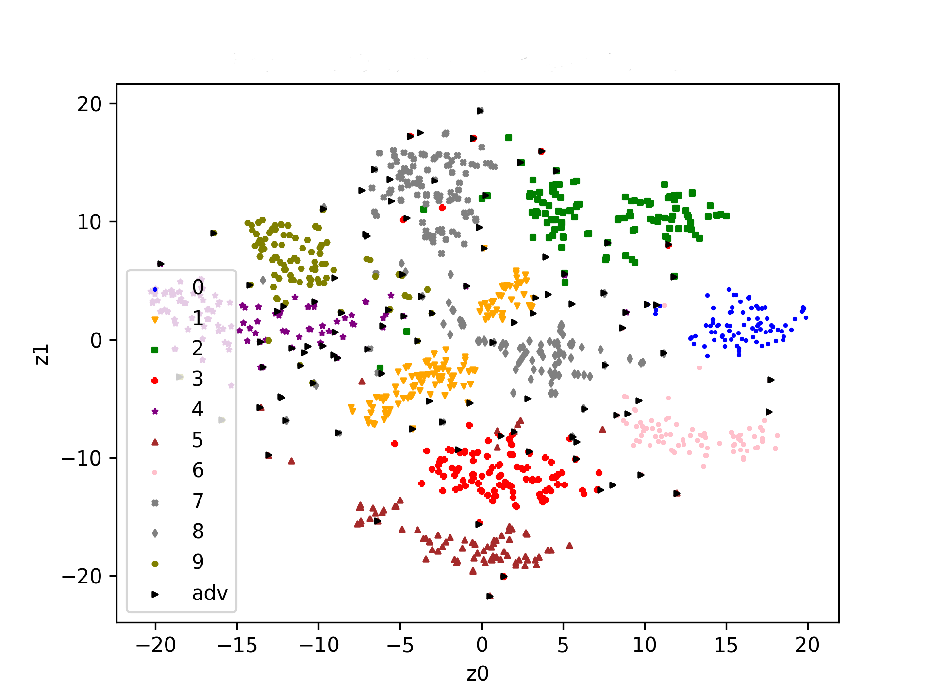
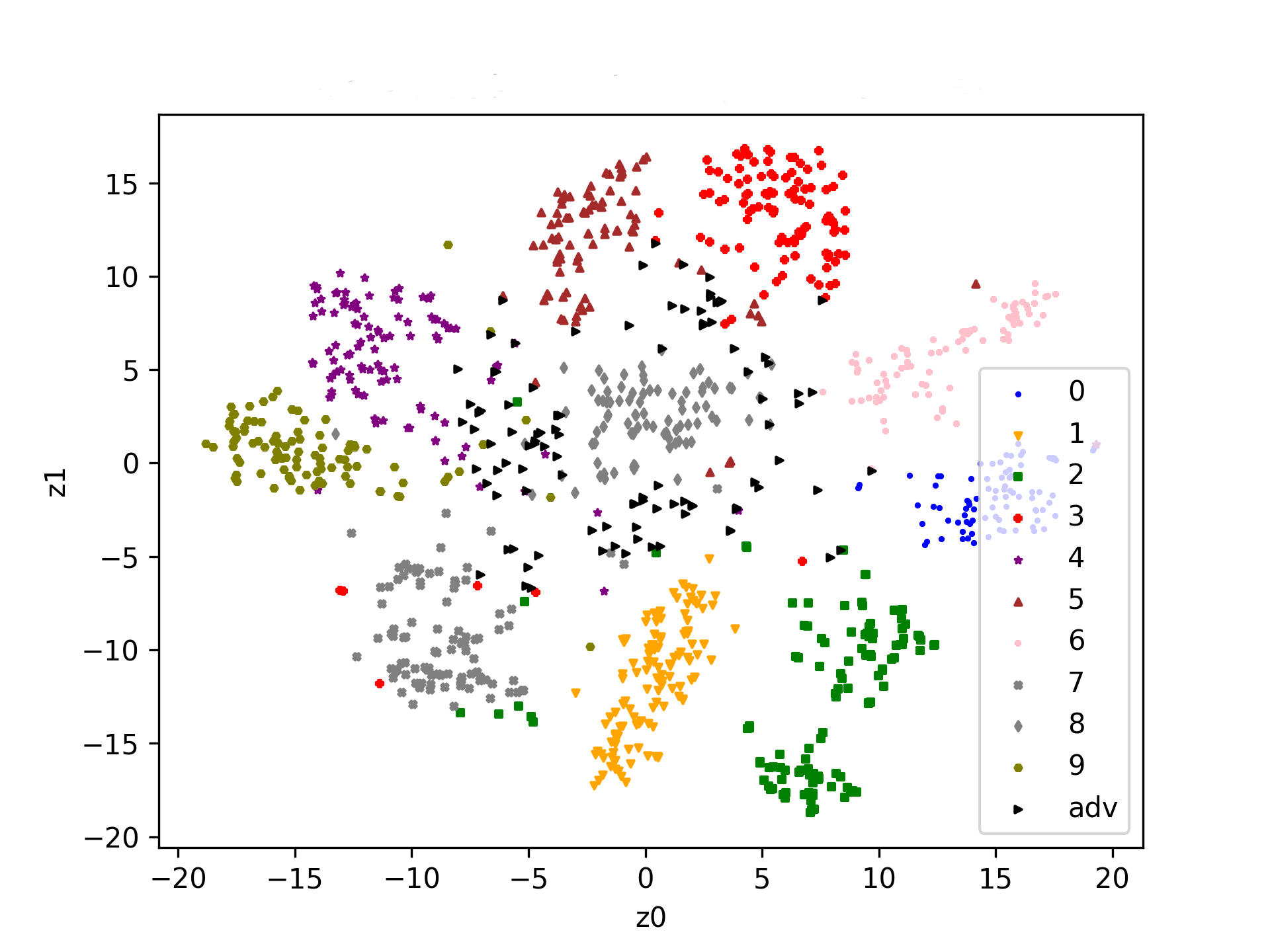
Figure 4: T-SNE visualization of latent space. Black triangles are (positive) adversarial examples while others are clean images. Left: ADR-None. Right: ADR+LC/GB

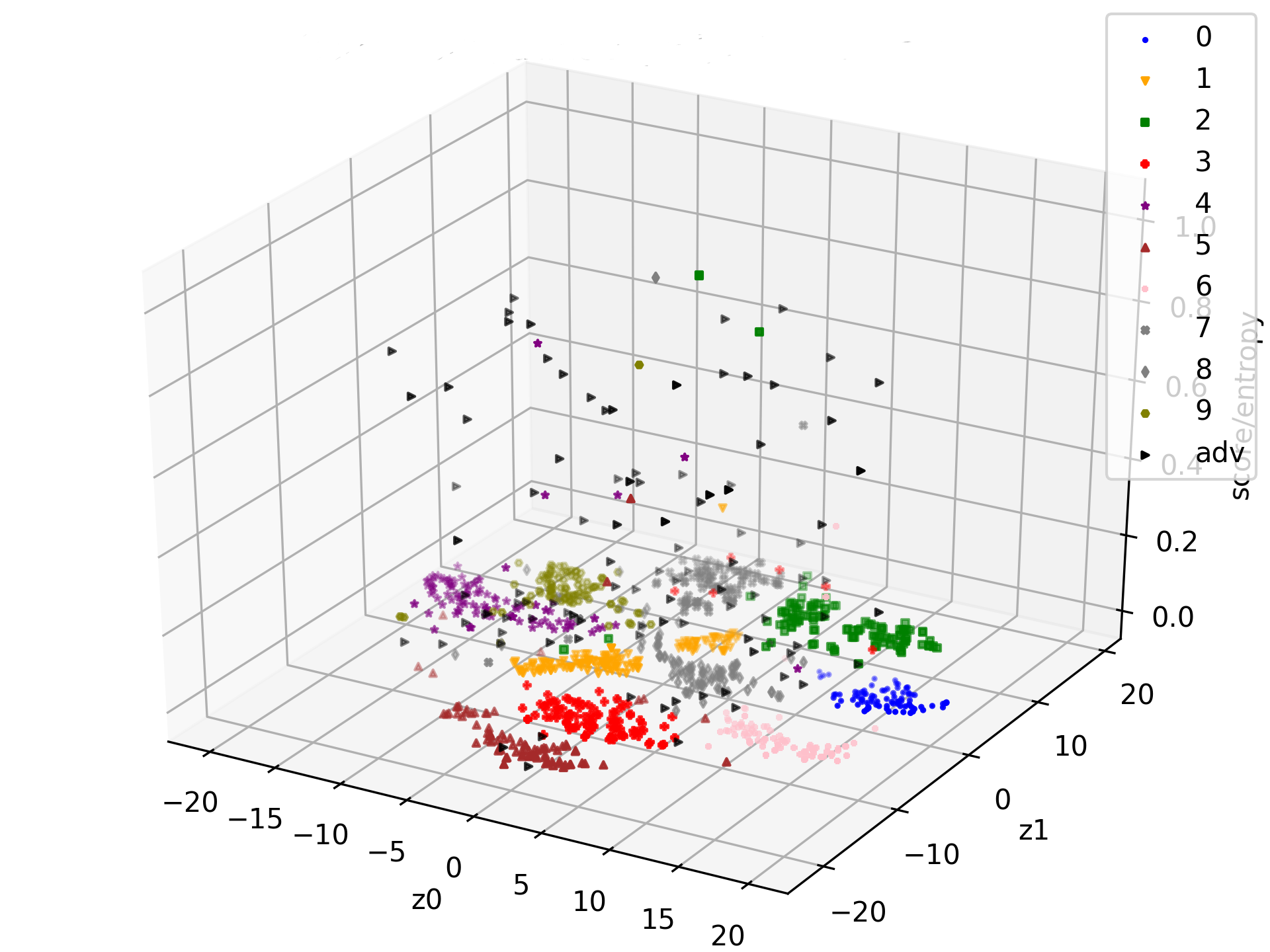
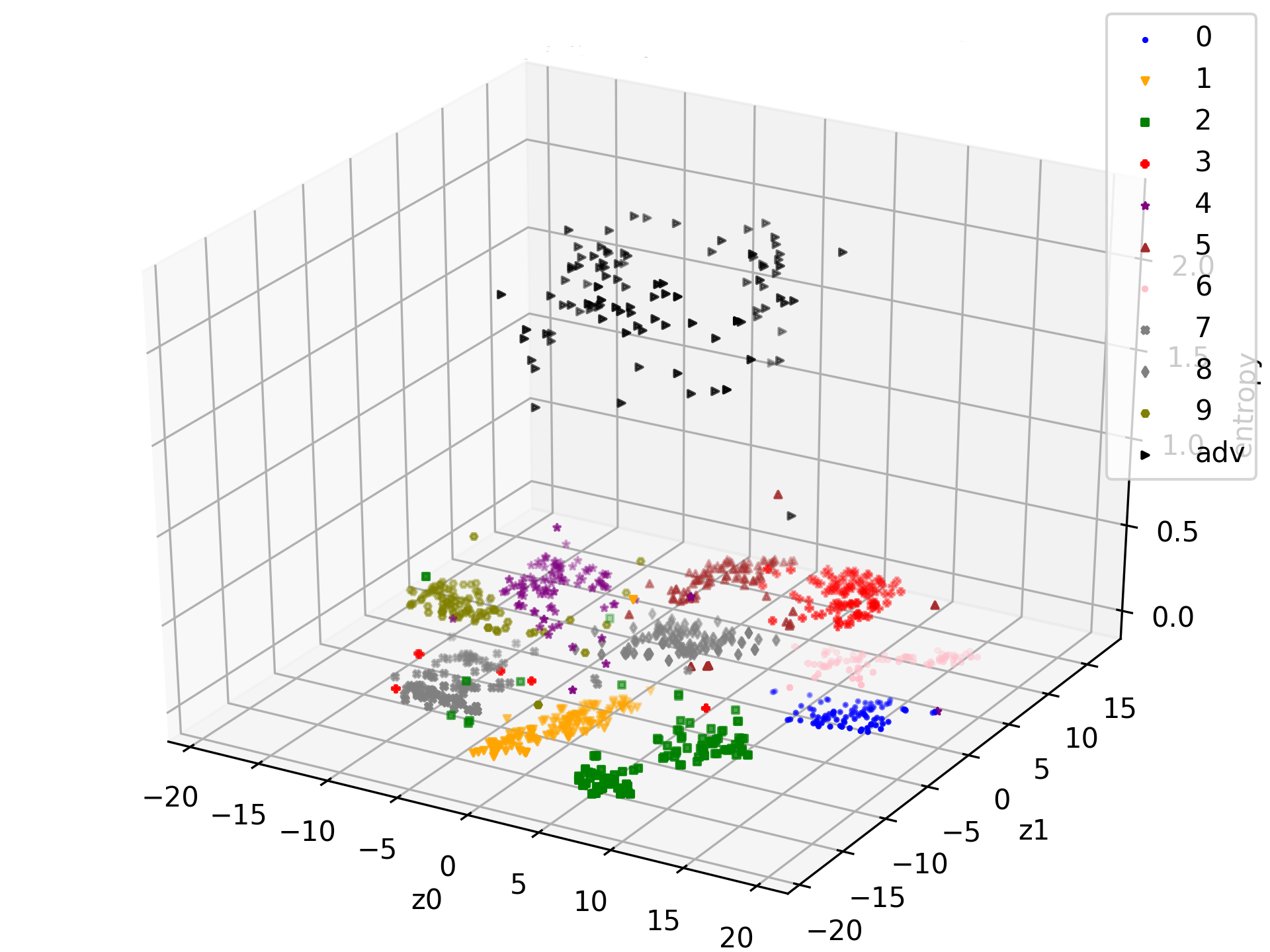
Figure 5: T-SNE visualization of latent space with entropy of the prediction probability. Black triangles are (positive) adversarial examples while others are clean images. Left: ADR-None. Right: ADR+LC/GB

To summarize, in this ablation study, we have demonstrated how our proposed components can improve adversarial robustness. In the next section, we will compare the best variant (with all components) of our method with both ADV and TRADES on more complex datasets to highlight the capability of our method.

4.2.2 Experiment on the MNIST dataset

We compare our method with ADV and TRADES on the MNIST dataset. For our method, in addition to using its full version with all of the proposed terms, we consider two variants ADR-ADV and ADR-TRADES wherein the adversary $\mathcal{A}$ is set to be ADV and TRADES respectively. We use PGD/TRADES generated adversarial examples with $k=20,\varepsilon_{d}=0.3,\eta_{d}=0.01$ for adversarial training as proposed in [19] and employ the PGD attack with $k=40$, using two iterative size $\eta\in\{0.01,0.02\}$ and different distortion boundaries $\varepsilon$ to attack. The results shown in Figure 6 illustrate that our variants outperform the baselines, especially for $\{\varepsilon=\varepsilon_{d}=0.3,\eta=0.01\}$. For example, our ADR-ADV improves ADV by 2.4% (from 94.15% to 96.55%) while ADR-TRADES boosts TRADES by 2.07% (from 93.64% to 95.71%). While for attack setting $\{\epsilon=\epsilon_{d}=0.3,\eta=0.02\}$, our method improves ADV and TRADES by 4.0% and 3.8% respectively. Moreover, the improvement gap increases when the attack goes stronger.

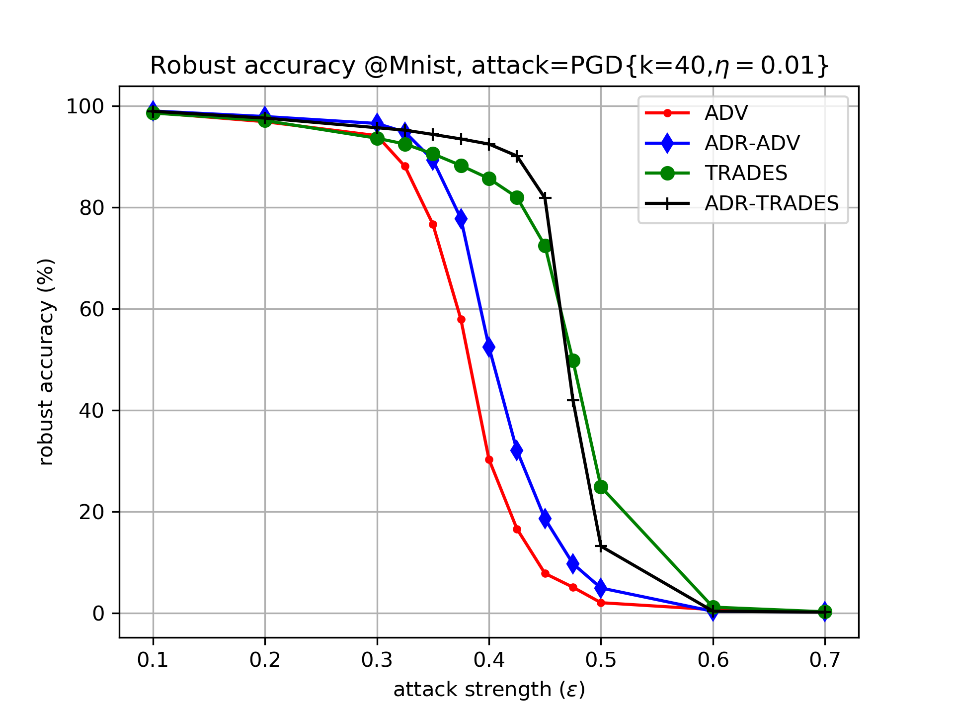
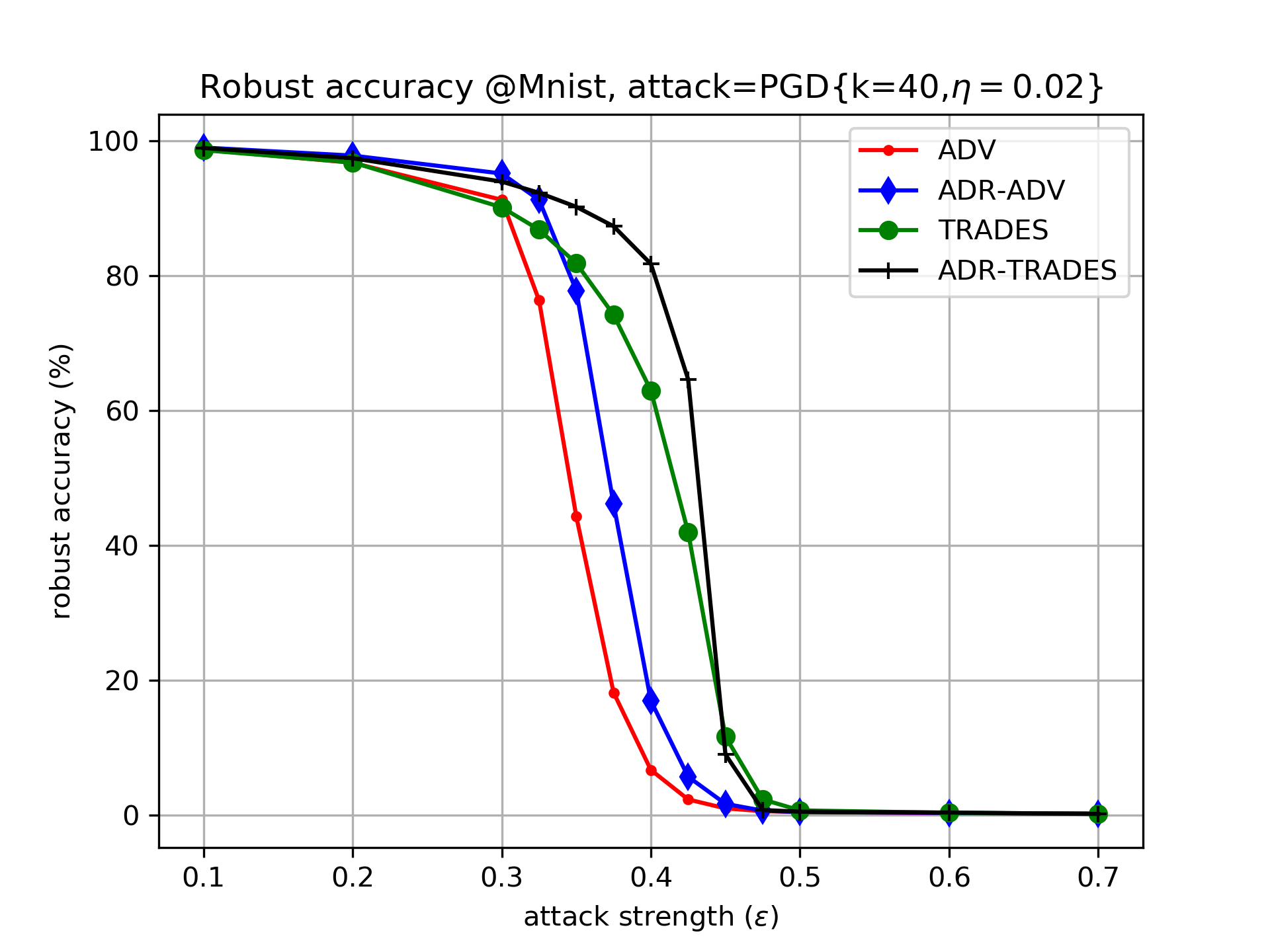
Figure 6: Robust accuracy against PGD attack on MNIST. Base models include ADV and TRADES. Left: $\eta=0.01$. Right: $\eta=0.02$

4.2.3 Experiment on the CIFAR-10 dataset

We conduct experiments on the CIFAR-10 dataset under two different architectures: standard CNN from [2] and ResNet from [19]. We set $k=10,\varepsilon_{d}=0.031,\eta_{d}=0.007$ for ADV and TRADES and use a PGD attack with $k=20$, $\eta\in\{0.0039,0.007\}$ and different distortion boundary $\varepsilon$. The results for standard CNN architecture in figure 7 show that our methods significantly improve over the baselines. Moreover, the results for standard CNN architecture at a checking point $\{\varepsilon=\varepsilon_{d}=0.031,\eta=\eta_{d}=0.007\}$ in Table 2 show that our methods significantly outperform their baselines in terms of natural and robust accuracies. Moreover, Figure 7 indicates that our proposed methods can defend better in a wide range of attack strength. Particularly, when with varied distortion boundary $\varepsilon$ in $\left[0.02,0.1\right]$, our proposed methods always produce better robust accuracies than its baselines. Finally, the results for ResNet architecture in Table 2 show a slight improvement of our methods comparing with ADV but around $2.5\%$ improvement from TRADES on both Non-targeted and Multi-targeted attacks. The quality of adversarial examples and the chosen network architecture obviously affects the overall performance, however, in this experiment, we empirically prove that our proposed components can boost the robustness under different combinations of the adversarial training frameworks and network architectures.

Table 2: Robustness comparison on the CIFAR-10 dataset against PGD attack at $k=20,\epsilon=0.031,\eta=0.007$ using Standard CNN and ResNet architectures

	Standard CNN				ResNet
	Nat. acc.	Non-target	Mul-target		Nat. acc.	Non-target	Mul-target
Standard model	75.27%	12.26%	0.00%		92.51%	0.00%	0.00%
ADV	67.86%	33.12%	18.73%		78.84%	44.08%	41.20%
TRADES	71.37%	35.84%	18.01%		83.27%	37.52%	35.05%
ADR-ADV	69.09%	37.67%	22.58%		78.43%	44.72%	41.43%
ADR-TRADES	69.0%	39.68%	26.7%		82.02%	40.17%	37.70%

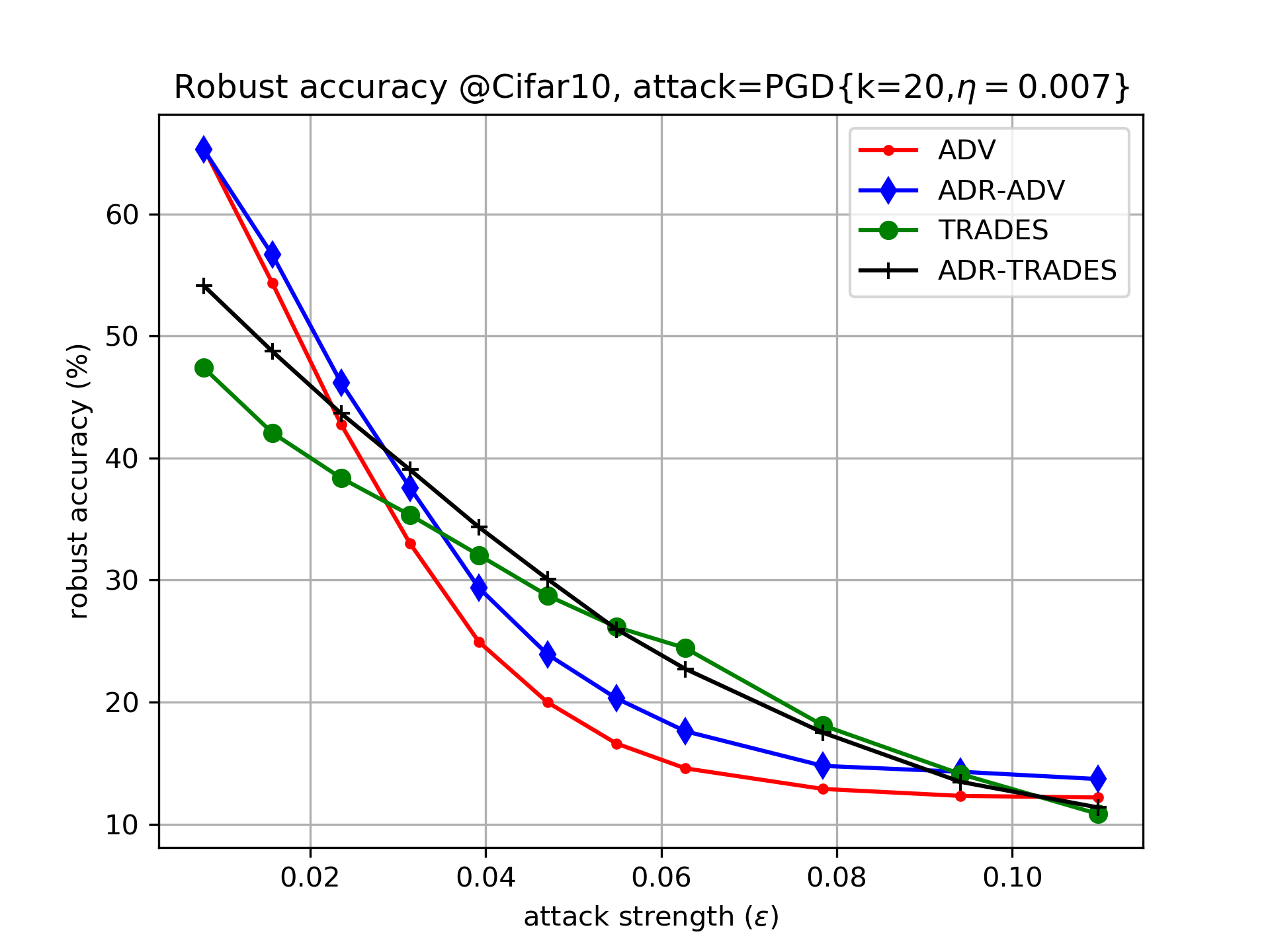
Figure 7: Robust accuracy against PGD attack on CIFAR-10, using Standard CNN architecture. Base models include ADV and TRADES. Left: $\eta=0.0039$. Right: $\eta=0.007$.

5 Conclusion

Previous studies have shown that adversarial training has been one of the few defense models resilient to various attack types against deep neural network models. In this paper, we have shown that by enforcing additional components, namely local/global compactness constraints together with the clustering assumption, we can further improve the state-of-the-art adversarial training models. We have undertaken comprehensive experiments to investigate the effect of each component and have demonstrated the capability of our proposed methods in enhancing adversarial robustness using real-world datasets.

Acknowledgement:

This work was partially supported by the Australian Defence Science and Technology (DST) Group under the Next Generation Technology Fund (NTGF) scheme.

Supplementary to “Improving Adversarial Robustness by Enforcing Local and Global Compactness”

6 Hyperparameters

The hyperparameters for our experiments as Table 3. The hyperparameters of local compactness, global compactness, and smoothness are set to be either 1 or 0, meaning they are switched ON/OFF. Although finer tuning of these parameters can lead to better results, our method outperforms the baselines in these initial settings, which demonstrates the effectiveness of those components.

Table 3: Hyper-parameter setting for the experiment section

	$\lambda_{com}^{lc}$	$\lambda_{com}^{gb}$	$\lambda_{smt}$	$\lambda_{conf}$
MNIST	1.	1.	1.	0.
CIFAR-10-CNN	1.	1.	1.	1.
CIFAR-10-ResNet	1.	1.	1.	0.

7 Model architectures and experimental setting

We summarize the experimental setting in Table 4.

Table 4: Experimental settings for our experiments. The model architectures are from [2] [19] and redescribed in the supplementary material.

		MNIST		CIFAR-10 (CNN)		CIFAR-10 (Resnet)
Architectures		CNN-4C3F(32)[2]		CNN-4C3F(64)[2]		RN-34-10[19]
Optimizer		SGD		Adam		SGD
Learning rate		0.01		0.001		0.1
Momentum		0.9		N/A		0.9
Training stratery		Batch size 128, 100 epochs		Batch size 128, 200 epochs		Batch size 128, 200 epochs
Perturbation		$k=20,\epsilon_{d}=0.3,\eta_{d}=0.01,l_{\infty}$		$k=10,\epsilon_{d}=0.031,\eta_{d}=0.007,l_{\infty}$		$k=10,\epsilon_{d}=0.031,\eta_{d}=0.007,l_{\infty}$

For the MNIST dataset, we used the standard CNN architecture with three convolution layers and three fully connected layers described in [2]. For the CIFAR-10 dataset, we used two architectures in which one is the standard CNN architecture described in [2] and another is the ResNet architecture used in [19]. The ResNet architecture has 5 residual units with (16, 16, 32, 64) filters each. We choose the convolution layers as the Generator and the last fully connected layers as the Classifier for ResNet architecture. The standard CNN architectures are redescribed as follow:

CNN-4C3F(32) Generator: 2$\times$Conv(32)$\rightarrow$ Max Pooling$\rightarrow$ 2$\times$Conv(32)$\rightarrow$ Max Pooling$\rightarrow$ Flatten

CNN-4C3F(32) Classifier: FC(200)$\rightarrow$ ReLU$\rightarrow$ Dropout(0.5)$\rightarrow$ FC(200)$\rightarrow$ ReLU$\rightarrow$ FC(10)$\rightarrow$ Softmax

CNN-4C3F(64) Generator: 2$\times$Conv(64)$\rightarrow$ Max Pooling$\rightarrow$ 2$\times$Conv(64)$\rightarrow$ Max Pooling$\rightarrow$ Flatten

CNN-4C3F(64) Classifier: FC(256)$\rightarrow$ ReLU$\rightarrow$ Dropout(0.5)$\rightarrow$ FC(256)$\rightarrow$ ReLU$\rightarrow$ FC(10)$\rightarrow$ Softmax

8 Choosing the intermediate layer

The intermediate layer for enforcing compactness constraints immediately follows on from the generator. We additionally conduct an ablation study to investigate the importance of choosing the intermediate layer and report natural accuracy and robust accuracy against non-targeted/multiple-targeted attacks respectively. We use the standard CNN architecture (which has 4 Convolution layers in Generator and 3 FC layers in Classifier), with four additional variants corresponding to different choices of the intermediate layer (right after the generator). We use PGD ($k=100,\epsilon=0.3,\eta=0.01$ for MNIST, $k=100,\epsilon=0.031,\eta=0.007$ for CIFAR-10) to evaluate these models. It can be seen from the results as showing in Table 5 that the performance slightly downgrades if choosing shallower layers. The higher impact is expected on a larger architecture (i.e., Resnet), which can be investigated in future.

Table 5: Performance comparison on different choices of the intermediate layer. The results in each setting are natural accuracy and robust accuracy against non-targeted/multiple-targeted attacks respectively.

		MNIST		CIFAR10
G=2Conv, C=2Conv+3FC		99.52/93.88/92.78		68.78/36.46/21.99
G=3Conv, C=1Conv+3FC		99.44/94.38/93.59		69.17/37.05/22.44
CNN (G=4Conv, C=3FC)		99.48/95.06/94.26		69.08/37.06/22.44
G=4Conv+1FC, C=2FC		99.51/94.38/93.47		69.39/37.31/22.87
G=4Conv+2FC, C=1FC		99.52/94.26/93.45		69.13/37.31/22.57

9 The performance of TRADES

TRADES aims to find the most divergent adversarial examples, while ADV aims to find the worst-case examples to improve a model (see Sec. 2.2 in our paper for more detail). Hence theoretically, there is no guarantee that TRADES outperforms ADV. In practice, the performance of TRADES is influenced by the classifier architectures and parameter tunings. The works [22, 11] also reported that TRADES cannot surpass ADV all the time (Table 1 and footnote 8 in [22], Table 1 in [11]), which is in line with the findings in our paper.

10 Further experiments

We conduct an additional evaluation with further state-of-the-art attack methods (e.g., the Basic Iterative Method - BIM [14] and the Momentum Iterative Method - MIM [6]) to convince that our method indeed boots the robustness rather than suffers the gradient obfuscation [1]. Three attack methods PGD, BIM and MIM share the same setting, i.e., $\{k=100,\epsilon=0.3,\eta=0.01\}$ for MNIST and $\{k=100,\epsilon=0.031,\eta=0.007\}$ for CIFAR-10. The result as in Table 6 show that our components can improve the robustness of the baseline framework against all three kind of attacks which again proves the efficacy of our method.

Table 6: Robustness comparison on the MNIST and CIFAR-10 datasets using Standard CNN with higher attack iteration (i.e., $k=100$). The results in each setting are natural accuracy and robust accuracy against non-targeted/multiple-targeted attacks respectively.

		Dataset		ADV		ADR-ADV
PGD		MNIST		99.43/93.13/92.09		99.48/95.06/94.26
BIM		MNIST		99.43/93.00/91.70		99.48/94.86/93.99
MIM		MNIST		99.43/94.05/92.63		99.48/95.41/94.56
PGD		CIFAR-10		67.61/32.87/18.74		69.16/36.85/22.71
BIM		CIFAR-10		67.61/32.89/18.71		69.16/36.82/22.69
MIM		CIFAR-10		67.61/33.00/18.59		69.16/36.96/22.56

10.1 Loss surface of adversarial examples

We separate adversarial examples into two classes: positive adversarial example which successfully fools a defense method and negative adversarial example which is an unsuccessful attack. The loss surface of positive adversarial example as Figure 8. In particular, both ADV (ADR-None) and our method (ADR+LC) predicted $x_{a}$ with the label 8, whereas its true label is 3. From Figure 8, it is evident that for ADV, that most of its neighborhood region is non-smooth, resulting in incorrect predictions in almost all of the grid. By contrast, for our method (ADR+LC), the loss surface w.r.t. the input is smoother, resulting in more correct predictions in this neighborhood region. In addition, in our method, the prediction surface w.r.t. the latent feature in the intermediate representation layer is smoother than that w.r.t. input. This means that our local compactness makes the local region more compact, hence improving adversarial robustness.

We provide the loss surface of negative adversarial examples from adversarial training method and adversarial training with our components as Figure 9. Both examples show that the loss function smooth in local region of an adversarial example.

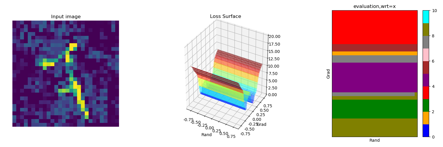
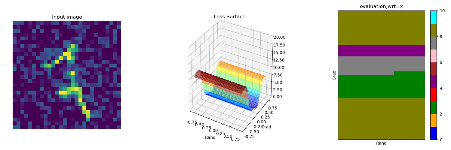
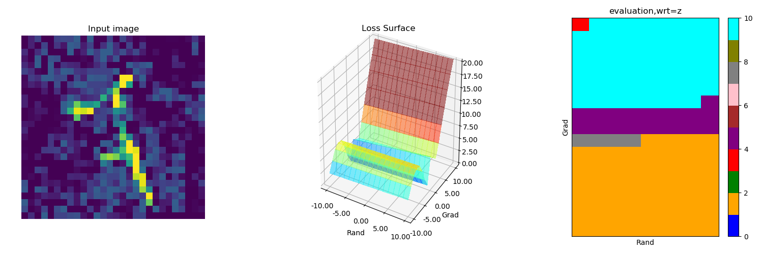
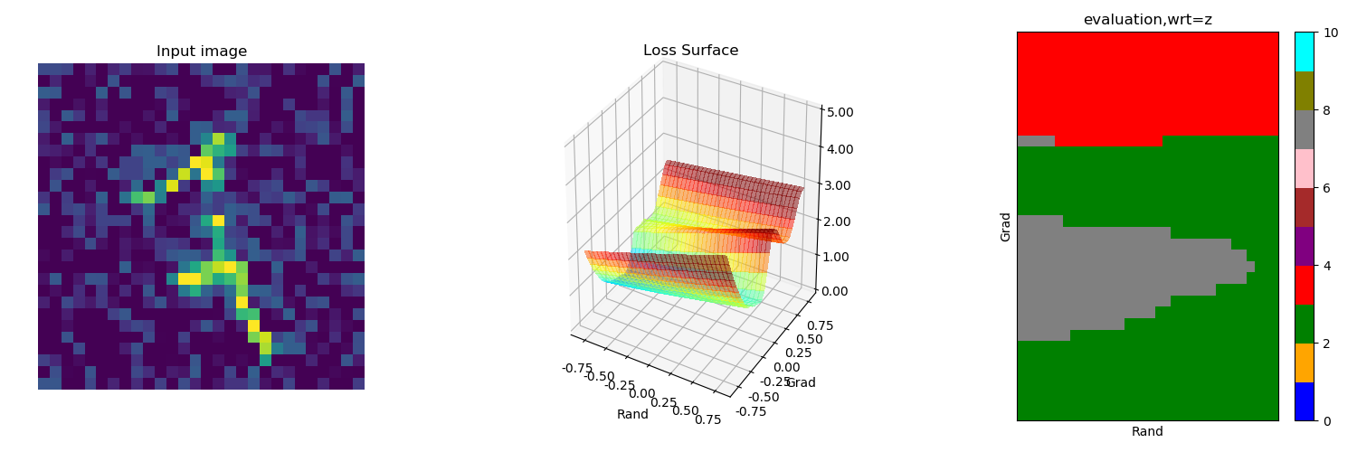
Figure 8: Loss surface at local region of a positive adversarial example. Top-left: ADR-None w.r.t input. Top-right: ADV+LC w.r.t input. Bottom-left: ADR-None w.r.t latent. Bottom-right: ADV+LC w.r.t latent

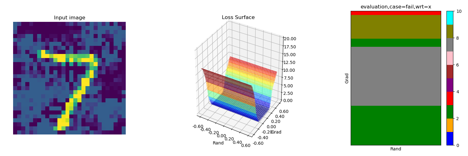
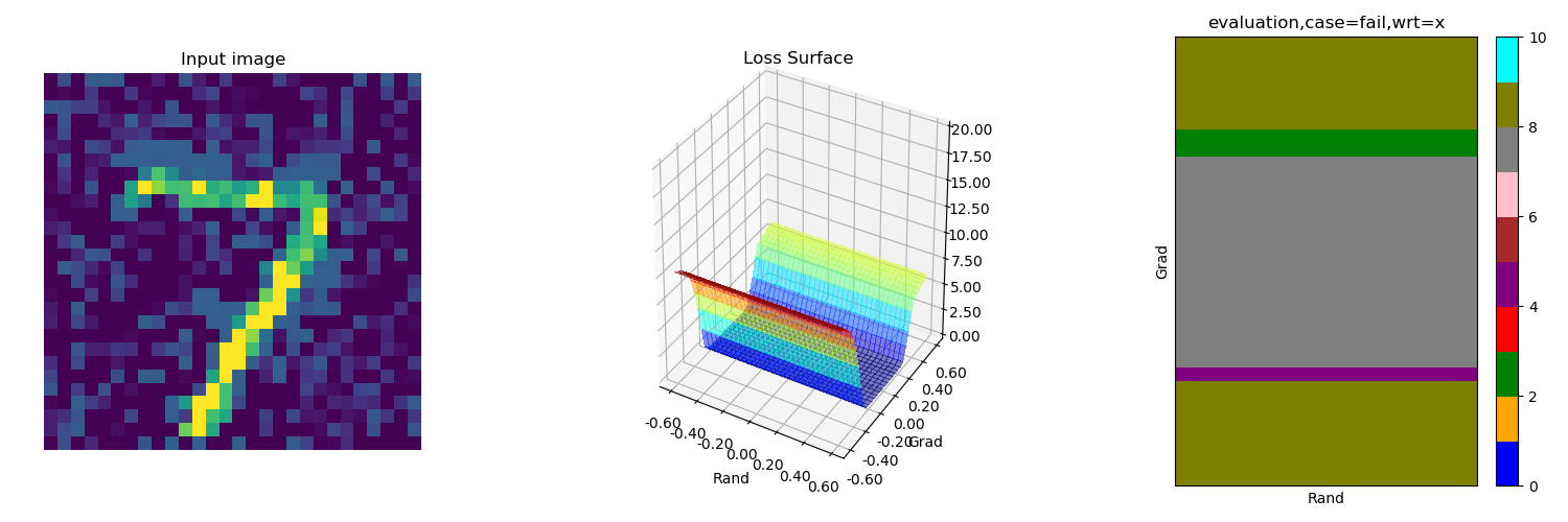
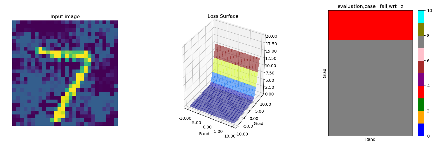
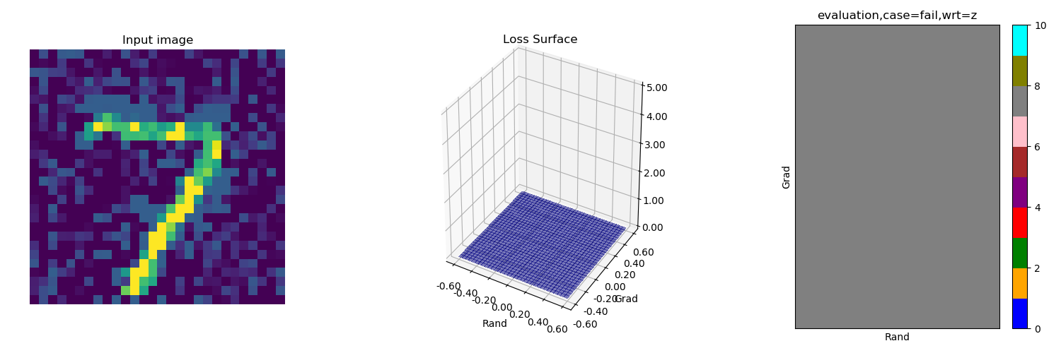
Figure 9: Loss surface at local region of a negative adversarial example. Top-left: ADR-None w.r.t input. Top-right: ADV+LC w.r.t input. Bottom-left: ADR-None w.r.t latent. Bottom-right: ADV+LC w.r.t latent

10.2 T-SNE visualization of adversarial examples

In addition to positive adversarial examples, we provide the t-SNE visualization of the negative adversarial examples from adversarial training (ADR-None) and adversarial training with our components (ADR+LC/GB) as Figure 10. In adversarial training method, the unsuccessful attacks have been mixed insight the natural/clean data. In contrast, in case adversarial training with our components, the attack representation consistently is separated from those from natural data, similar to positive adversarial examples. Additionally, the unsuccessful attacks in adversarial training have the same confidence level with natural data, while those in our methods are totally different levels. In summary, our method can produce a better latent representation which is well separated between natural data and adversarial example (both positive and negative). This feature can be used for adversarial detection.

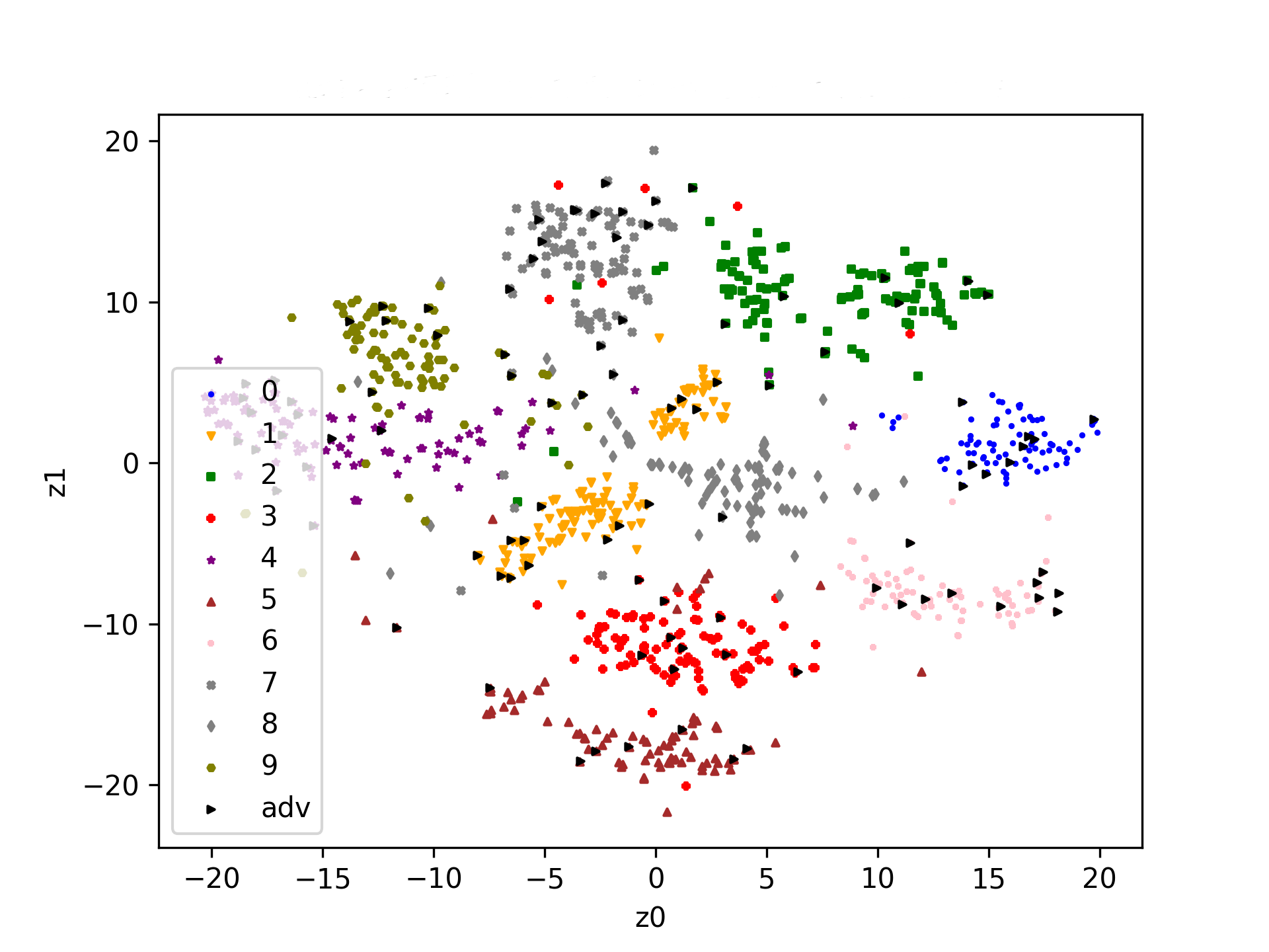
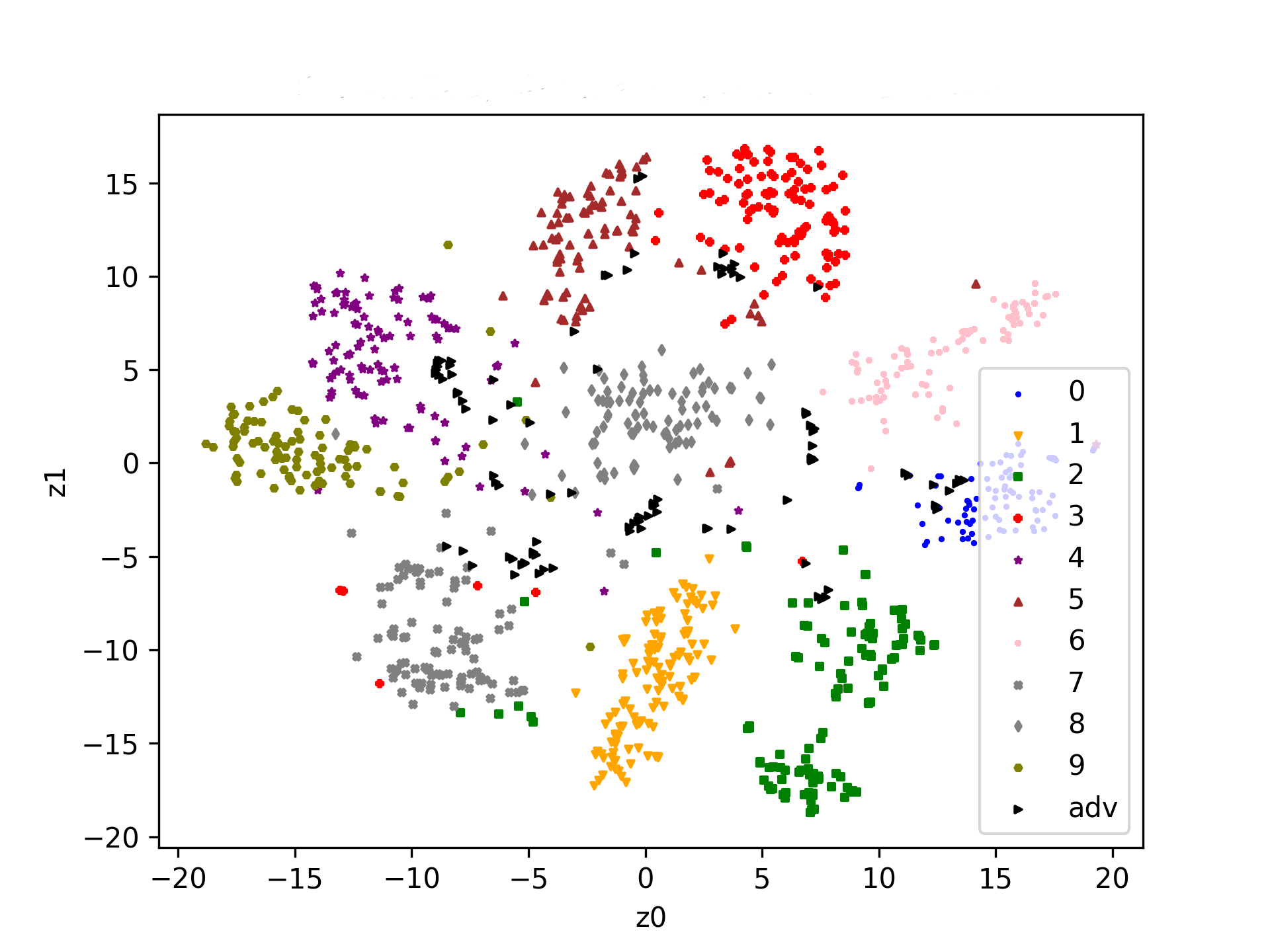
Figure 10: T-SNE visualization of latent space. Black triangles are (negative) adversarial examples while others are clean images. Left: ADR-None. Right: ADR+LC/GB

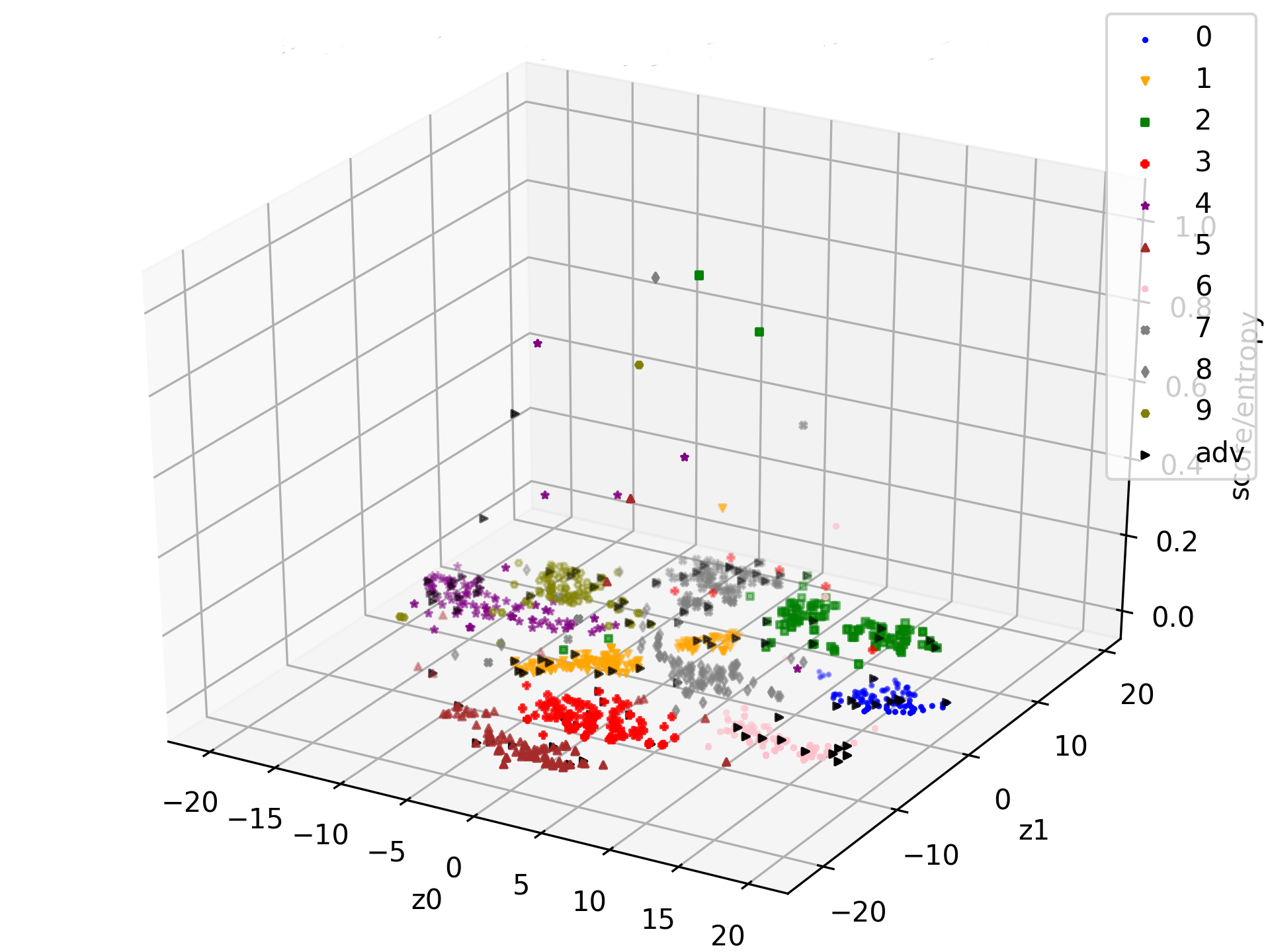
Figure 11: T-SNE visualization with entropy of prediction with entropy of prediction probability. Black triangles are (negative) adversarial examples while others are clean images. Left: ADR-None. Right: ADR+LC/GB

References

- [1] Athalye, A., Carlini, N., Wagner, D.: Obfuscated gradients give a false sense of security: Circumventing defenses to adversarial examples. arXiv preprint arXiv:1802.00420 (2018)
- [2] Carlini, N., Wagner, D.: Towards evaluating the robustness of neural networks. In: 2017 ieee symposium on security and privacy (sp). pp. 39–57. IEEE (2017)
- [3] Chapelle, O., Zien, A.: Semi-supervised classification by low density separation. In: AISTATS. vol. 2005, pp. 57–64 (2005)
- [4] Chen, T., Kornblith, S., Norouzi, M., Hinton, G.: A simple framework for contrastive learning of visual representations. arXiv preprint arXiv:2002.05709 (2020)
- [5] Dhillon, G.S., Azizzadenesheli, K., Lipton, Z.C., Bernstein, J., Kossaifi, J., Khanna, A., Anandkumar, A.: Stochastic activation pruning for robust adversarial defense. arXiv preprint arXiv:1803.01442 (2018)
- [6] Dong, Y., Liao, F., Pang, T., Su, H., Zhu, J., Hu, X., Li, J.: Boosting adversarial attacks with momentum. In: Proceedings of the IEEE conference on computer vision and pattern recognition. pp. 9185–9193 (2018)
- [7] Goodfellow, I.J., Shlens, J., Szegedy, C.: Explaining and harnessing adversarial examples. arXiv preprint arXiv:1412.6572 (2014)
- [8] Gulrajani, I., Ahmed, F., Arjovsky, M., Dumoulin, V., Courville, A.C.: Improved training of wasserstein gans. In: Advances in neural information processing systems. pp. 5767–5777 (2017)
- [9] He, K., Fan, H., Wu, Y., Xie, S., Girshick, R.: Momentum contrast for unsupervised visual representation learning. In: Proceedings of the IEEE/CVF Conference on Computer Vision and Pattern Recognition. pp. 9729–9738 (2020)
- [10] Jakubovitz, D., Giryes, R.: Improving dnn robustness to adversarial attacks using jacobian regularization. In: Proceedings of the European Conference on Computer Vision. pp. 514–529 (2018)
- [11] Jalal, A., Ilyas, A., Daskalakis, C., Dimakis, A.G.: The robust manifold defense: Adversarial training using generative models. arXiv preprint arXiv:1712.09196 (2017)
- [12] Kannan, H., Kurakin, A., Goodfellow, I.: Adversarial logit pairing. arXiv preprint arXiv:1803.06373 (2018)
- [13] Krizhevsky, A., et al.: Learning multiple layers of features from tiny images (2009)
- [14] Kurakin, A., Goodfellow, I., Bengio, S.: Adversarial examples in the physical world. arXiv preprint arXiv:1607.02533 (2016)
- [15] Kurakin, A., Goodfellow, I., Bengio, S.: Adversarial machine learning at scale. arXiv preprint arXiv:1611.01236 (2016)
- [16] LeCun, Y., Bottou, L., Bengio, Y., Haffner, P.: Gradient-based learning applied to document recognition. Proceedings of the IEEE 86(11), 2278–2324 (1998)
- [17] Lin, J., Gan, C., Han, S.: Defensive quantization: When efficiency meets robustness. arXiv preprint arXiv:1904.08444 (2019)
- [18] Maaten, L.v.d., Hinton, G.: Visualizing data using t-sne. Journal of machine learning research 9(Nov), 2579–2605 (2008)
- [19] Madry, A., Makelov, A., Schmidt, L., Tsipras, D., Vladu, A.: Towards deep learning models resistant to adversarial attacks. arXiv preprint arXiv:1706.06083 (2017)
- [20] Miyato, T., Maeda, S., Koyama, M., Ishii, S.: Virtual adversarial training: A regularization method for supervised and semi-supervised learning. IEEE Transactions on Pattern Analysis and Machine Intelligence 41(8), 1979–1993 (Aug 2019)
- [21] Oord, A.v., Kalchbrenner, N., Kavukcuoglu, K.: Pixel recurrent neural networks. arXiv preprint arXiv:1601.06759 (2016)
- [22] Qin, C., Martens, J., Gowal, S., Krishnan, D., Dvijotham, K., Fawzi, A., De, S., Stanforth, R., Kohli, P.: Adversarial robustness through local linearization. In: Advances in Neural Information Processing Systems. pp. 13824–13833 (2019)
- [23] Samangouei, P., Kabkab, M., Chellappa, R.: Defense-gan: Protecting classifiers against adversarial attacks using generative models. arXiv preprint arXiv:1805.06605 (2018)
- [24] Shafahi, A., Najibi, M., Ghiasi, M.A., Xu, Z., Dickerson, J., Studer, C., Davis, L.S., Taylor, G., Goldstein, T.: Adversarial training for free! In: Advances in Neural Information Processing Systems. pp. 3353–3364 (2019)
- [25] Shu, R., Bui, H.H., Narui, H., Ermon, S.: A dirt-t approach to unsupervised domain adaptation. arXiv preprint arXiv:1802.08735 (2018)
- [26] Song, Y., Kim, T., Nowozin, S., Ermon, S., Kushman, N.: Pixeldefend: Leveraging generative models to understand and defend against adversarial examples. arXiv preprint arXiv:1710.10766 (2017)
- [27] Szegedy, C., Zaremba, W., Sutskever, I., Bruna, J., Erhan, D., Goodfellow, I., Fergus, R.: Intriguing properties of neural networks. arXiv preprint arXiv:1312.6199 (2013)
- [28] Xie, C., Wu, Y., Maaten, L.v.d., Yuille, A.L., He, K.: Feature denoising for improving adversarial robustness. In: Proceedings of the IEEE Conference on Computer Vision and Pattern Recognition. pp. 501–509 (2019)
- [29] Zhang, H., Yu, Y., Jiao, J., Xing, E.P., Ghaoui, L.E., Jordan, M.I.: Theoretically principled trade-off between robustness and accuracy. arXiv preprint arXiv:1901.08573 (2019)