Space-Time Smoothing of Demographic and Health Indicators using the R Package SUMMER

Zehang Richard Li Space-Time Smoothing of Demographic and Health Indicators using the R Package SUMMER SUMMER: Space-Time Smoothing of Demographic and Health Indicators The increasing availability of complex survey data, and the continued need for estimates of demographic and health indicators at a fine spatial and temporal scale, which leads to issues of data sparsity, has led to the need for spatio-temporal smoothing methods that acknowledge the manner in which the data were collected. The open source R package SUMMER implements a variety of methods for spatial or spatio-temporal smoothing of survey data. The emphasis is on small-area estimation. We focus primarily on indicators in a low and middle-income countries context. Our methods are particularly useful for data from Demographic Health Surveys and Multiple Indicator Cluster Surveys. We build upon functions within the survey package, and use INLA for fast Bayesian computation. This paper includes a brief overview of these methods and illustrates the workflow of accessing and processing surveys, estimating subnational child mortality rates, and visualizing results with both simulated data and DHS surveys. Bayesian, small area estimation, survey sampling, mortality, DHS, INLA Bayesian, small area estimation, survey sampling, mortality, DHS, INLA Zehang Richard Li
University of California, Santa Cruz
Baskin Engineering, MS SOE 2, 1156 High St, Santa Cruz CA, USA
E-mail:
URL: https://zehangli.com
 

1 Introduction

A wealth of health and demographic indicators are now collected across the world, and interest often focuses on patterns in space and time. Spatial patterns indicate potential disparities while temporal trends are important for determining the impact of interventions and to assess whether targets, such as the sustainable development goals (SDGs) are being met (macfeely:20). In low- and middle-income countries (LMIC) the most reliable data with sufficient spatial resolution are often collected under complex sampling designs, an aspect that must be acknowledged in the analysis to reduce bias and obtain proper uncertainty measures in the prevalence estimates. A crucial assumption (rao:molina:15, Section 4.3) is that the probability of selection of a unit, given covariates, does not depend on the values of the response, which is sometimes known as ignorability. Common sources of data include the Demographic Health Surveys (DHS) and Multiple Indicator Cluster Surveys (MICS), both of which use multi-stage cluster sampling. We describe a common two-stage cluster design. A sampling frame of clusters (for example, enumeration areas) is constructed, often from a census, and then strata are formed. The strata consist of some administrative geographical partition crossed with urban/rural (with countries having their own definitions of this dichotomy). Then a pre-specified number of clusters are sampled from these strata under some probabilistic scheme, for example, with probability proportional to size (PPS). Different surveys are powered to different geographical levels. Then, within the selected clusters, households are randomly sampled and individuals are sampled within these households, and asked questions on a range of health and demographic variables.

The SUMMER package provides a computational framework and a collection of tools for smoothing and mapping the prevalence of health and demographic indicators with complex survey data over space and time. Smoothing is important to avoid unstable estimates and combine information from multiple surveys over time. Originally developed for small area estimation (SAE) of the under-5 child mortality rate (U5MR), the SUMMER package has been extended to more general tasks in prevalence mapping. The implemented methods have already been successfully applied to a range of data, e.g., subnational estimates of U5MR (mercer:etal:15; li:etal:19), HIV prevalence (wakefield:okonek:pedersen:20) and vaccination coverage (dong:wakefield:20). Recently, the SUMMER package was used to obtain the official United Nations Inter-Agency Group for Mortality Estimation (UN IGME) yearly estimates (1990–2018) of U5MR at administrative level $2$ below the national level (admin-2 estimates) for 22 countries in Africa and Asia. Previously, the UN IGME only produced national estimates using the B3 model (alkema:new:14). The results of these endeavors will be available online at https://childmortality.org.

The main focus of this paper is to provide an overview of the different models and a hands-on tutorials to implement these models through several case studies. Various other packages are available within R for SAE, including the sae package (molina:marhuenda:15) that supports the popular book of rao:molina:15, and includes the famous fay:herriot:79 model and spatial smoothing options. A more comprehensive list of related packages are described at https://cran.r-project.org/web/views/OfficialStatistics.html. An important distinction in SAE is between area-level and unit-level models. The area-level approach (fay:herriot:79) directly models an area-level variable, such as a weighted estimate. In contrast, unit-level models (battese:etal:88) are specified at the level of the sampling unit, which are clusters in the examples we consider.

The rest of the paper is organized as follows. In Section 2, we briefly describe the different smoothing models implemented in SUMMER. We then provide an overview of the SUMMER package in Section 3. Section 4 to LABEL:sec:malawi provides a series of examples with increasing complexity. We first demonstrate the spatial and space-time smoothing of a generic binary indicator collected though complex survey sampling in Section 4. We then demonstrate the more complex functionalities of estimating mortality rates including the neonatal mortality rate (NMR) and U5MR in Section 5. The analysis in these two Sections use simulated data that are included in the SUMMER package. In Section LABEL:sec:malawi we describe the complete workflow of estimating U5MR using the two most recent DHS surveys from Malawi and in Section LABEL:sec:vis we illustrate various visualization tools provided in the SUMMER package and provide a brief consideration of model checking. We discuss future work in Section LABEL:sec:discuss.

2 Space-time smoothing using complex survey data

In this section we review different methods to estimate the prevalence of a health outcome from complex survey data. We begin by discussing design-based, direct estimates (rao:molina:15) which are based on response data from that area only. Next, we describe space-time smoothing of the direct estimates, predictably we term these smoothed direct estimates. The first considers the case where the prevalence of a single binary indicator, e.g., disease and vaccination status, is of interest, and then extends the methods to the more complicated case of composite indicators such as the U5MR. We then describe a unit-level model to estimate prevalence at finer spatial and temporal resolutions.

2.1 Estimating the prevalence of a generic binary indicator

Consider a study region that is partitioned into $n$ areas, with interest focusing on estimating the prevalence of a binary indicator in each area, possibly over time. The data are collected via some complex survey design. For each individual $j$, let $y_{j}$ denote the individual’s outcome, and $w_{j}$ denote the design weight associated with this individual. Further, let $s_{it}$ represent the indexes of individuals sampled in area $i$ and in time period $t$. The design-based estimator (horvitz:thompson:52; hajek:71) is

$$\hat{p}_{it}^{\texttt{HT}}=\frac{\sum_{j\in s_{it}}w_{j}y_{j}}{\sum_{j\in s_{it}}w_{j}}.$$ (1)

This is an example of a direct estimate. The variance of $\hat{p}_{it}^{\texttt{HT}}$ can be calculated using standard methods (wolter:07). Let $V^{\texttt{HT}}_{it}$ denote the design-based variance of $\mbox{logit}(p_{it}^{\texttt{HT}})$, obtained from the design-based variance of $p_{it}^{\texttt{HT}}$ via linearization (the delta method). We take the direct estimates as input data and estimate the true prevalence with the random effects model,

$$\mbox{logit}(\hat{p}_{it}^{\texttt{HT}})|\lambda_{it} \sim\mbox{Normal}(\lambda_{it},V^{\texttt{HT}}_{it}),$$ (2)

$$\lambda_{it} =\mbox{\boldmath$x$}_{it}^{\intercal}\mbox{\boldmath$\beta$}+\alpha_{t}+\epsilon_{t}+S_{i}+e_{i}+\delta_{it}.$$ (3)

In this model, which is a space-time smoothing extension of the fay:herriot:79 model, $\mbox{expit}(\lambda_{it})$ is the true prevalence we aim to estimate, and $\mbox{\boldmath$x$}_{it}$ are areal-level covariates that are potentially time-varying. The rest of the terms are normally distributed random effects including structured time trends $\alpha_{t}$, unstructured, independent and identically distributed (iid), temporal terms $\epsilon_{t}$, structured spatial trends $S_{i}$, unstructured spatial terms $e_{i}$, and space-time interaction terms $\delta_{it}$. The terms $e_{i}+S_{i}$ are implemented via the BYM2 parameterization (riebler:etal:16), a reparameterization of the classical BYM model (besagbayesian) that combines iid error terms with intrinsic conditional autoregressive (ICAR) random effects. Several different temporal models are implemented in SUMMER for the structured temporal trends and space-time interaction effects, including random walks of order 1 and 2, and autoregressive models (rue:knorrheld:05) with additional linear trends. The interaction term $\delta_{it}$ can be one of the type I to IV interactions of the chosen temporal model and the ICAR model in space, as described in knorrheld:00. In order for the model to be identifiable, we impose sum-to-zero constraints on each group of random effects. More details on the prior choices are provided in Section 2.4.

2.2 Estimating the U5MR using area-level models

For composite indicators such as U5MR, the direct estimates require additional modeling. The SUMMER package implements the discrete hazards model described in mercer:etal:15. In this subsection, we focus on the estimation of U5MR. The functions in SUMMER can be adapted to model mortality rates of other age groups as well. In practice, while modeling the NMR or death in the first year of life will often be feasible, subnational modeling of mortality beyond age 5 is more challenging because death becomes rarer, and survey data alone are not sufficient for reliable inference. Following previous work (mercer:etal:15), we use discrete time survival analysis to estimate age-specific monthly probabilities of dying in user-defined age groups. We assume constant hazards within the age bands. The default choice uses the monthly age bands

$$[0,1),[1,12),[12,24),[24,36),[36,48),[48,60)$$

for U5MR. Hence, using a synthetic cohort approach, the U5MR for area $i$ and time $t$ can be calculated as,

$$\hat{p}_{it}^{\texttt{HT}}=\tensor*[_{60}]{\hat{q}}{{}^{it}_{0}}=1-\prod_{a=1}^{6}\left(1-\tensor*[_{n_{a}}]{\hat{q}}{{}^{it}_{x_{a}}}\right)$$ (4)

where $x_{a}$ and $n_{a}$ are the start and end of the $a$-th age group, and $\tensor*[_{n_{a}}]{q}{{}^{it}_{x_{a}}}$ is the probability of death in age group $[x_{a},x_{a}+n_{a})$ in area $i$ and time $t$, with $\tensor*[_{n_{a}}]{\hat{q}}{{}^{it}_{x_{a}}}$ the estimate of this quantity. The constant one-month hazards in each age band can be estimated by fitting a weighted logistic regression model (binder:83):

$$\mbox{logit}\left(\tensor*[_{1}]{q}{{}^{it}_{m}}\right)=\beta_{a[m]}^{it},$$ (5)

where

$$a[m]=\left\{\begin{array}[]{ll}1&\mbox{if }m=0,\\ 2&\mbox{if }m=1,\dots,11,\\ 3&\mbox{if }m=12,\dots,23,\\ 4&\mbox{if }m=24,\dots,35,\\ 5&\mbox{if }m=36,\dots,47,\\ 6&\mbox{if }m=48,\dots,59.\end{array}\right.$$ (6)

The design-based variance of $\mbox{logit}(\hat{p}_{it}^{\texttt{HT}})$ may then be estimated using the delta method although resampling methods such as the jackknife can also be used (pedersenandliu:2012). The smoothing of the direct estimates can then proceed using the model described in equations (2)–(3). When multiple surveys exist, one may choose to either model the survey-specific effects as fixed or random (for example, mercer:etal:15 describe a random effects model) or first aggregate the direct estimates from multiple surveys to obtain a ‘meta-analysis’ estimate in each area and time period (li:etal:19). To mitigate the sparsity of available data in each year, li:etal:19 also considers a temporal model defined at the yearly level while the direct estimates are calculated at multi-year periods. All these variations can be fit using the SUMMER package.

2.3 Estimating the U5MR with cluster-level models

The smoothed direct estimates are useful when there are enough observations at the spatial and temporal unit of the analysis. When the target of inference is at finer resolution, e.g., on a yearly time scale with admin-2 areas and surveys stratified at admin-1 levels, the direct estimates may contain many $0$s or $1$s and the design-based variance cannot be calculated reliably. In this case, we can consider model-based approaches at the cluster level. We describe the model for the mortality estimation problem below, while the same formulation applies to the case of any generic binary indicators as well.

In the most general setting, we consider multiple surveys over time, indexed by $k$. The sampling frame that was used for survey $k$, will be denoted by $r[k]$. We assume a discrete hazards model as before. We consider a beta-binomial model for the probability (hazard) of death from month $m$ to $m+1$ in survey $k$ and at cluster location $\mbox{\boldmath$s$}_{c}$ in year $t$. This model allows for overdispersion relative to the binomial model. Assuming constant hazards within age bands, we assume the number of deaths occurring within age band $a[m]$, in cluster $c$, time $t$, and survey $k$ follow the beta-binomial distribution,

$$Y_{a[m],k,c,t}~{}|~{}p_{a[m],k,c,t}\sim\mbox{BetaBinomial}\left(~{}n_{a[m],k,c,t}~{},~{}p_{a[m],k,c,t}~{},d~{}\right),$$ (7)

where $p_{a[m],k,c,t}$ is the monthly hazard within age band $a[m]$, in cluster $c$, time $t$, and survey $k$ and $d$ is the overdispersion parameter. The latent logistic model we use is,

$$p_{m,k,c,t}= \mbox{expit}(\alpha_{m,c,k,t}+\epsilon_{t}+b_{k})$$ (8)

$$\alpha_{m,k,c,t}= \beta_{a^{\star}[m],r[k],t}I(s_{c}\in\mbox{ rural })+\gamma_{a^{\star}[m],r[k],t}I(s_{c}\in\mbox{ urban })$$

$$\;+S_{i[s_{c}]}+e_{i[s_{c}]}+\delta_{i[s_{c}],t}+\mbox{BIAS}_{k,t}$$ (9)

This form consists of a collection of terms that are used for prediction and a number that are not, as we now describe. We include a survey fixed effect $b_{k}$ with the constraint $\sum_{k}b_{k}\mathbf{1}_{r[k]=r}=0$ for each sampling frame $r$, so that the main temporal trends are identifiable for each sampling frame. The $b_{k}$ terms are not included in the prediction, i.e., they are set to zero. The $\epsilon_{t}$ are unstructured temporal effects that allow for perturbations over time. It is a contextual choice whether they are used in predictions. We include terms in (9) that are analogous to those in equations (2)–(3), in particular the spatial main effects $S_{i}$ and $e_{i}$ and the space-time interactions $\delta_{it}$. For the temporal main effects $\beta_{a^{\star}[m],r[k],t}$ and $\gamma_{a^{\star}[m],r[k],t}$, we have stratum-specific distinct random walks for each age group $a^{\star}[m]$ in surveys from each sampling frame. We include separate urban and rural temporal terms to acknowledge the sampling design, often urban clusters are oversampled and have different risk to rural clusters, and so it is important to acknowledge this aspect in the model (paige:etal:20). The urban-rural stratification effects may also be parameterized as time-invariant fixed effects, i.e., restricting $\beta_{a^{\star}[m],r[k],t}=\gamma_{a^{\star}[m],r[k],t}+\Delta_{a^{\star}[m],r[k]}$. We use $a^{\star}[m]$ here to differentiate from the age bands used in the hazard likelihood. We may link the month $m$ to a reduced number of age bands $a$ that are expected to have different temporal trends. The default choice in the package is

$$a^{\star}[m]=\left\{\begin{array}[]{ll}1&\mbox{if }m=0,\\ 2&\mbox{if }m=1,\dots,11,\\ 3&\mbox{if }m=12,\dots,59.\end{array}\right.$$ (10)

In situations where biases are known for particular surveys and/or years, we can adjust for bias following wakefield:etal:19 by including the bias ratio term,

$$\mbox{BIAS}_{k,t}=\frac{\mbox{U5MR}^{\star}_{t}}{\widehat{\mbox{U5MR}}_{k,t}},$$

where $\mbox{U5MR}^{\star}_{t}$ is the expected U5MR in year $t$ and $\widehat{\mbox{U5MR}}_{k,t}$ is the biased version. This approach has been used to adjust for mothers who have died from AIDS (walker:etal:12); such mothers cannot be surveyed, and their children are more likely to have died, so the missingness is informative.

The predicted U5MRs in urban and rural regions of area $i$ and at time $t$ according to sampling frame $r$ are,

$$\mbox{U5MR}_{i,t,U,r} = 1-\prod_{a=1}^{6}\left[\frac{1}{1+\exp(\beta_{a,r,t}+S_{i}+e_{i}+\delta_{i,t})}\right]^{z[a]}$$ (11)

$$\mbox{U5MR}_{i,t,R,r} = 1-\prod_{a=1}^{6}\left[\frac{1}{1+\exp(\gamma_{a,r,t}+S_{i}+e_{i}+\delta_{i,t})}\right]^{z[a]},$$ (12)

where $z[a]=1,11,12,12,12,12$, for the default choice of age bands. The aggregate risk in area $i$ and in year $t$ according to sampling frame $r$ is

$$p_{itr}=q_{itr}\times\mbox{U5MR}_{i,t,U,r}+(1-q_{itr})\times\mbox{U5MR}_{i,t,R,r},$$ (13)

where $q_{itr}$ and $1-q_{itr}$ are the proportions of the under-5 population in area $i$ that are urban and rural in year $t$ according to the classification of sampling frame $r$. The final aggregation over different sampling frames can be done using meta-analysis combination, so that,

$$\widehat{\mbox{U5MR}}_{it}=\mbox{expit}\left(\sum_{r}w_{itr}\times\mbox{logit}(p_{itr})\right),$$

where $w_{itr}=U_{itr}^{-1}/\sum_{r^{\prime}}U_{itr^{\prime}}^{-1}$ is the scaled inverse of $U_{itr}$, which is the posterior variance of $\mbox{logit}(\widehat{\mbox{U5MR}}_{it}^{(r)})$. Beyond point estimates, we obtain the full posterior of $\mbox{U5MR}_{it}$, and various summaries can be reported or mapped. The estimate constructed for U5MR is not relevant to any child, because that child would have to experience the hazards for each age group simultaneously in time period $t$, rather than moving through age groups over multiple time periods. Nevertheless, the resultant U5MR is a useful summary and the conventional measure that is used to inform on child mortality.

2.4 Prior specification

In all the model implementations, we apply penalised complexity (PC) priors to model the random effects (simpson:etal:17). These priors are proper and parameterization invariant. The basis of PC priors is to regard each model component as a flexible extension of a so-called base model. Considering an unstructured iid model component, the base model would be to remove this component from the linear predictor by letting its variance parameter go to zero. This is also the base model for any simple Gaussian model component with mean zero. The main idea is to follow Occam’s razor and favor less complex, or more intuitive, models unless the data suggest otherwise. Of note, state-of-the-art priors, such as the inverse gamma prior for a variance parameter, put zero density mass at the base model and as such do not allow the recovery of this model. The PC prior is specified by following a number of desirable principles and is derived based on the Kullback-Leibler distance of the flexible model from the base model. For details we refer to simpson:etal:17. Here, we will shortly comment on the PC priors relevant for the parameters used in our models and their default hyperparameters. All the PC priors can be specified by the user in the function calls using arguments such as pc.u and pc.alpha.

Considering a simple Gaussian model component with standard deviation parameter $\sigma$, the PC prior results in an exponential distribution for $\sigma$. The rate parameter $\lambda_{\sigma}$ can be informed using a probability contrast of the form $\mbox{Prob}(\sigma>U_{\sigma})=\alpha_{\sigma}$, which leads to $\lambda_{\sigma}=-\log(\alpha_{\sigma})/U_{\sigma}$ (simpson:etal:17). The SUMMER package uses as default $U_{\sigma}=1$ and $\alpha_{\sigma}=0.01$, which means that the 99th percentile of the prior is at 1.

For the structured spatial random effects, we use the BYM2 model (riebler:etal:16; simpson:etal:17). It has a structured and unstructured term, and uses a single variance, $\sigma^{2}$, that represents the marginal spatial variance and a mixing parameter $\phi\in[0,1]$ specifying the proportion of spatial variation. To interpret $\sigma$ as a marginal standard deviation, the spatial component in (3) needs to be scaled, so that $\mbox{Var}(e_{i})\approx\mbox{Var}(S_{i})\approx 1$. This leads to:

$$\mathbf{e}+\mbox{\boldmath$S$}=\sigma(\sqrt{(1-\phi)}\mathbf{e}^{\star}+\sqrt{\phi}\mbox{\boldmath$S$}^{\star})$$

where $\mathbf{e}^{\star}$ is iid normally distributed with fixed variance equal to 1 and $\mbox{\boldmath$S$}^{\star}$ is the scaled ICAR model. We follow riebler:etal:16 and scale the ICAR component so that the geometric mean of the marginal variances of $S_{i}$ is equal to 1. Note that we also apply this scaling procedure to all intrinsic model components, such as random walk of order 1 or 2 components (sorbye-rue-2014), to ensure interpretability of the prior distributions assigned to their flexibility parameters. The BYM2 model has a two-stage base model, with the first implying the absence of any spatial effect by setting $\sigma$ equal to zero, and the second by assuming $\phi=0$ and therefore only unstructured spatial variation. For $\sigma$ we use an exponential prior as outlined before. The prior for $\phi$ depends on the study-specific neighborhood graph and is not available in closed form, see riebler:etal:16 for details. Its hyperparameter $\lambda_{\phi}$ can be derived from $\mbox{Prob}(\phi<U_{\phi})=\alpha_{\phi}$. The SUMMER package uses as default $U_{\phi}=0.5$ and $\alpha_{\phi}=2/3$, which means that the 66.6th percentile of the prior is at 0.5, so that values of $\phi$ less than $0.5$ are preferred a little more, a priori.

For the autoregressive model for time effects, we again use an exponential prior for the marginal standard deviation. For the autocorrelation correlation coefficient $\omega$, we assume as base model $\omega=1$. This represents a limiting random walk which assumes that the process does not change in time. The prior for $\omega$ is again not available in closed form, see sorbye:rue:17 for details. Its hyperparameter $\lambda_{\omega}$ can be found from $\mbox{Prob}(\omega>U_{\omega})=\alpha_{\omega}$. The SUMMER package uses as default $U_{\omega}=0.7$ and $\alpha_{\omega}=0.9$, which means that the 10th percentile of the prior is at 0.7, and therefore preferring values of $\phi$ that are close to 1.

The space-time interaction terms, $\delta_{it}$, are modeled with the Type I, II, III, IV models of knorrheld:00. The Type I model assumes iid interaction terms, the Type II model that the interactions are temporally structured but independent in space and the Type III model that the interactions are iid in time but spatially structured via an ICAR model. For the default Type IV interaction, we assume the specified temporal model and spatial (ICAR) structured effects interact. When the temporal component in the space-time interaction terms are modeled with a random walk of order 1 or an autoregressive model of order 1, we may also allow area-specific deviations from the main temporal trends by letting $\delta_{it}=b_{i}t+\delta_{it}^{\star}$, where $\delta_{it}^{\star}$ follows the specified interaction model and $b_{i}$ are random slopes. This allows us to capture more flexible temporal dynamics, and may aid in area-specific predictions. The random slopes are modeled with a Gaussian prior. To facilitate interpretation, we scale the time index to be from $-0.5$ to $0.5$, so that the random slope can be interpreted as the total deviation from the main time trend from the first and last years to be projected, on the logit scale. Users can specify priors for the random slopes with the PC prior so that $\mbox{Prob}(|b|<U_{b})=\alpha_{b}$ using arguments pc.st.slope.u and pc.st.slope.alpha.

3 Overview of SUMMER and the workflow

The SUMMER package provides a collection of functions for SAE with complex survey data. The package is available via the Comprehensive R Archive Network (CRAN) and can be directly installed in R by

R> install.packages("SUMMER")

The SUMMER package requires the INLA package (rue:etal:09) to be installed. All analysis in this package are conducted with SUMMER package version $1.0.0$ and INLA version $20.03.17$. INLA can be installed with

R> install.packages("INLA", repos=c(getOption("repos"), R> INLA="https://inla.r-inla-download.org/R/stable"), dep=TRUE)

The SUMMER package consists of three main functions to fit the space-time smoothing models:

• smoothSurvey produces direct and smoothed direct estimates for a generic binary indicator from raw survey data using methods described in Section 2.1.

• smoothDirect also produces the smoothed direct estimates, with more features in the model components that are particularly relevant to mortality estimation introduced in li:etal:19 and touched upon in Section 2.2. Unlike smoothSurvey, smoothDirect takes pre-calculated direct estimates as input, and thus allows more flexibility for handling composite indicators.

• smoothCluster performs cluster-level smoothing using methods described in Section 2.3.

The main source of data required for these methods are the survey data and the corresponding spatial polygons. For cluster-level modeling, we need additional information on which region each cluster belongs to. In the DHS, cluster locations are usually recorded in a separate GPS file, though strictly we do not need to know the GPS, rather just the strata in which each cluster lies. For mortality estimation, most of the data processing steps can be done with functions in SUMMER, as demonstrated in Section LABEL:sec:malawi. Figure 1 shows schematically the workflow of data processing and smoothing mortality estimates using the SUMMER package.

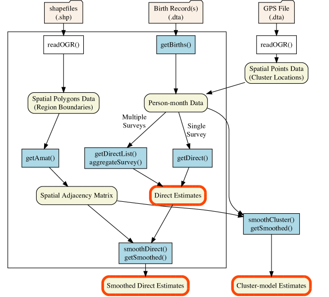
Figure 1: Workflow of estimating child mortality using the SUMMER package. Rounded blocks represent data types and rectangular blocks represent functions. Functions in the SUMMER package are colored in blue. Output estimates are highlighted in the boxes with red borders. The workflow in the group on the left produces smoothed direct estimates as described in more detail in li:etal:19

4 Estimating the prevalence of a binary indicator

We start by considering the model described in Section 2.1. We first demonstrate estimating NMR in a simulated dataset using the smoothSurvey function. Since NMR is a special case of the composite mortality indicator, we can also use the combination of functions presented in Figure 1 to obtain the estimates. This alternative approach is discussed in Section 5.

We first load the packages for the analysis, data processing and visualization. For the analysis presented in this paper, we use the ggplot2 package (wickham:ggplot2) and patchwork package (patchwork) to make further customizations of the visualization tools in SUMMER, and the dplyr package (dplyr) for processing DHS data in Section LABEL:sec:malawi.

R> library(SUMMER) R> library(ggplot2) R> library(patchwork) R> library(dplyr)

We load the DemoData dataset from the SUMMER package. The DemoData is a list that contains full birth history data from simulated surveys with stratified cluster sampling design, similar to most of the DHS surveys. It has been pre-processed into the person-month format, where for each list entry, each row represents one person-month record. Each record contains columns for the cluster ID (clustid), household ID (id), strata membership (strata) and survey weights (weights). The region and time period associated with each person-month record has also been computed and saved in the dataset. In this analysis, we use only the first survey.

R> data(DemoData) R> dat.one.surv <- DemoData[[1]] R> head(dat.one.surv)

clustid id region time age weights strata died 1 1 1 eastern 00-04 0 1.1 eastern.rural 0 2 1 1 eastern 00-04 1-11 1.1 eastern.rural 0 3 1 1 eastern 00-04 1-11 1.1 eastern.rural 0 4 1 1 eastern 00-04 1-11 1.1 eastern.rural 0 5 1 1 eastern 00-04 1-11 1.1 eastern.rural 0 6 1 1 eastern 00-04 1-11 1.1 eastern.rural 0

Since we are interested in estimating NMR, we only consider the survival in the first month for each child as a binary indicator. The age variable in this data frame are in the form of $a_{1}$-$a_{2}$, i.e., $1$-$11$ corresponds to age group with 1 to 11 completed months, whereas age groups with only one month are stored using a single number representation, e.g., age group $0$. This is also the data structure in the output of the getBirths function in the SUMMER package. We first create a smaller dataset containing only observations corresponding to the first month after birth during the period 2005–2009. The resulted two datasets have the common data structure from surveys where each row contains the records of one individual.

R> dat.one.surv <- subset(dat.one.surv, age=="0") R> dat.one.period <- subset(dat.one.surv, time == "05-09")

We first consider the smoothing model in equation (3) with only spatial terms. This model can be estimated with the smoothSurvey function. The function takes the survey data, spatial adjacency matrix, and variables specifying the column names in the data that correspond to response, region name, strata ID, cluster ID formula, and survey weights. In this example, we use the adjacency matrix from DemoMap$Amat$. The column and row names of the adjacency matrix need to be the same and match those in the region column in the data. In this example, there are four regions with the following adjacency matrix.

R> data(DemoMap) R> DemoMap$Amat\par\CodeOutput centraleasternnorthernwesterncentral0111eastern1010northern1101western1010\par Thestrata,clusterIDformula,andsurveyweightsusethesyntaxofthe\code{svydesign}functioninthe\pkg{survey}package\cite[citep]{(\@@bibref{AuthorsPhrase1Year}{lumley2004analysis}{\@@citephrase{, }}{})}.Inthisexample,wespecifythePCprioronthestandarddeviationsoftherandomeffectswith$U=1,\alpha=0.1$,whichcorrespondsto$\mbox{Prob}(\sigma>1)=0.1$.\par\CodeChunk\par\CodeInput R>fit.space<-smoothSurvey(data=dat.one.surv,Amat=DemoMap$Amat,R+responseType="binary",responseVar="died",R+regionVar="region",strataVar="strata",R+weightVar="weights",clusterVar="~{}clustid+id",R+pc.u=1,pc.alpha=0.1)\par Thedirectandsmootheddirectestimatesaresavedasdataframesinthereturnedobjects.Noticethatsincetheanalysisisperformedonthelogitoftheprevalence,estimatesonboththelogitandtheprobabilityscalesarereturnedintheoutput.Thesmootheddirectestimatesundergoshrinkageandhavesmallermarginalvariances.\par\CodeChunk\par\CodeInput R>fit.space$HT\par\CodeOutput regionHT.estHT.varHT.logit.estHT.logit.varHT.logit.prec1central0.0310.00016-3.40.1795.62eastern0.0670.00029-2.60.07413.63northern0.0480.00033-3.00.1596.34western0.0640.00036-2.70.1029.8\par\CodeChunk\par\CodeInput R>fit.space$smooth[,1:8]\par\CodeOutput regionmeanvarmedianlowerupperlogit.meanlogit.var1central0.0500.000170.0490.0250.076-3.00.0852eastern0.0600.000160.0580.0400.089-2.80.0473northern0.0540.000160.0530.0310.082-2.90.0634western0.0580.000170.0570.0370.089-2.80.054\par Wenowextendtheanalysisof\code{dat.one.surv}intheprevioussubsectiontothecaseofsmoothinginbothspaceandtime.Theonlydifferencefromtheuseof\code{smoothSurvey}previouslyistheadditionof\code{timeVar},whichspecifiesthetimeindexcolumn,togetherwith\code{time.model}and\code{type.st},whichspecifiesthetemporalmodelandinteractionmodeltouse.Intheanalysisbelow,weusearandomwalkoforder1astheprioronthestructuredtemporaleffect,withatypeIVspace-timeinteraction\cite[citep]{(\@@bibref{AuthorsPhrase1Year}{knorrheld:00}{\@@citephrase{, }}{})}.Thefittedobjecthasthesamedatastructureasbeforewithmultipleestimatesineachregioncorrespondingtothesixtimeperiods.\par\CodeChunk\par\CodeInput R>periods<-c("85-89","90-94","95-99","00-04","05-09","10-14")R>dat.one.surv$time.id<-match(dat.one.surv$time,periods)R>fit.st<-smoothSurvey(data=dat.one.surv,Amat=DemoMap$Amat,R+responseType="binary",responseVar="died",R+regionVar="region",strataVar="strata",R+weightVar="weights",clusterVar="~{}clustid+id",R+timeVar="time.id",time.model="rw2",type.st=4)\par$

5 Space-time smoothing of mortality rates

The smoothing of a generic binary indicator is a special case of the smoothing model described in Section 2.2. Thus we can smooth NMR in space and time using the workflow described in Figure 1 as well, with more flexible control over the model components. In this section, we first consider the space-time smoothing of NMR described in Section 4 but allowing the temporal random effects to be defined on yearly levels rather than in five-year periods. We then fit the cluster-level model for NMR, with the same data. Finally, we move beyond binary indicators and estimate U5MR with both smoothed direct and cluster-level models using multiple surveys. Throughout this section, we uses the simulated person-month data included in the SUMMER package.

5.1 Direct and smoothed direct estimates of NMR

We first use the getDirect function to calculate direct estimates using the discrete survival model described in mercer:etal:15. The function requires an input data frame of person-month record. The person-month record data can be created from birth records files from DHS or similar surveys using the getBirths function, which we demonstrate in Section LABEL:sec:malawi. The getDirect function returns a data frame of the direct estimates. Regions without deaths are returned with NA values in this data frame since direct estimates cannot be calculated.

R> direct.nmr <- getDirect(births = dat.one.surv, years = periods, R+ regionVar = "region", timeVar = "time", R+ clusterVar = " clustid + id", ageVar = "age", R+ weightsVar = "weights") R> direct.nmr[1:10, 1:8]

region years mean lower upper logit.est var.est region_num 1 All 85-89 0.134 0.0456 0.335 -1.9 0.36 0 2 All 90-94 NA NA NA NA NA 0 3 All 95-99 0.086 0.0407 0.172 -2.4 0.16 0 4 All 00-04 0.025 0.0102 0.062 -3.6 0.22 0 5 All 05-09 0.066 0.0338 0.127 -2.6 0.13 0 6 All 10-14 0.045 0.0228 0.086 -3.1 0.13 0 7 central 85-89 NA NA NA NA NA 1 8 central 90-94 NA NA NA NA NA 1 9 central 95-99 0.029 0.0039 0.184 -3.5 1.07 1 10 central 00-04 NA NA NA NA NA 1

The direct estimates obtained from getDirect are then fed into the smoothDirect function. The argument year_label specifies the order of the years column in the direct estimates, so that it does not have to be integer valued, and can easily allow extensions to future and past time periods not in the data. We can also fit the temporal model at the yearly level even though the direct estimates are in five year periods (li:etal:19). In this case we need to specify the proper range of the time periods (year_range) encoded by the time periods in year_label, and the number of years in each period $m$. Unequal periods are not supported at this time.

R> fit.st2 <- smoothDirect(data = direct.nmr, Amat = DemoMap