Formation of dispersive shock waves in a saturable nonlinear medium

Abstract

We use the Gurevich-Pitaevskii approach based on the Whitham averaging method for studying the formation of dispersive shock waves in an intense light pulse propagating through a saturable nonlinear medium. Although the Whitham modulation equations cannot be diagonalized in this case, the main characteristics of the dispersive shock can be derived by means of an analysis of the properties of these equations at the boundaries of the shock. Our approach generalizes a previous analysis of step-like initial intensity distributions to a more realistic type of initial light pulse and makes it possible to determine, in a setting of experimental interest, the value of measurable quantities such as the wave-breaking time or the position and light intensity of the shock edges.

1 Introduction

The propagation of nonlinear waves in dispersive media has attracted much attention in various fields of research such as water waves, plasma physics, nonlinear optics, Bose-Einstein condensates and others. In particular, the expansion of an initial state with a fairly smooth and large profile is accompanied by gradual steepening followed by wave breaking resulting in the formation of a dispersive shock wave (DSW), and this phenomenon was experimentally observed, for example, in Bose-Einstein condensates Dut01 ; secscb-05 ; hacces-06 and nonlinear optics gcrt-07 ; ggfdc-12 ; wmktcc-16 ; Xu2017 ; mbgc-17 ; nfxmef-19 . In these systems, the dynamics of the pulse is well described by the nonlinear Schrödinger (NLS) or Gross-Pitaevskii equation and the initial stage of evolution admits a purely hydrodynamic description in terms of the classical Riemann method, see, e.g., Refs. For2009 ; ik-19 ; ikp-19a ; ikp-19b ; ikp-19c . After the wave breaking moment, when DSWs are formed, the evolution of the wave structure can be described by the Whitham method Whitham-65 ; Whitham-74 ; kamch-2000 ; eh-16 . In the case of cubic Kerr-like nonlinearity the NLS equation is completely integrable, hence the Whitham modulation equations can be put in a diagonal Riemann form fl86 ; pavlov87 , and, with the use of the Gurevich-Pitaevskii approach gp-73 , it has been possible to develop a detailed analytic theory of the evolution of DSWs gk-87 ; eggk-95 ; ek-95 ; ikp-19a . This produces an excellent description of experiments wmktcc-16 ; Xu2017 on evolution of initial discontinuities in the intensity distribution of optical pulses propagating in optical fibers.

As first understood by Sagdeev Moi63 in the context of viscous stationary shocks whose width is much greater that a typical soliton width, the formation of DSWs is a universal phenomenon which occurs in a number of systems demonstrating nonlinear dispersive waves. In particular, the formation of DSWs has been observed in the propagation of light beams through a photorefractive medium cmc-04 ; wjf-07 . However, in such a system the nonlinearity is not of the Kerr type, and the theory of Refs. gk-87 ; eggk-95 ; ek-95 ; ikp-19a thus needs to be modified. Of course, the validity of the Whitham averaging approach for the description of the modulations of a nonlinear wave does not depend on the complete integrability of the wave equation. Nevertheless, it is difficult to put it into practice for non-completely integrable equations because of the lack of diagonalized form of the Whitham modulation equations.

The first general statement about the properties of DSWs applicable to a non-integrable situation was made by Gurevich and Meshcherkin in Ref. gm-84 . In this work the authors claimed that, when a DSW is formed after wave breaking of a “simple wave”, that is of a wave for which one of the non-dispersive Riemann invariants is constant, then the value of this constant Riemann invariant remains the same at both extremities of the DSW. In other words, this means that such a wave breaking leads to the formation of a single DSW, at variance with the situation with viscous shocks where more complicated wave structures are generated (see, e.g., Ref. LL-6 ). The next important step was made by El El-05 who showed that, in situations of the Gurevich-Meshcherkin type, when the Whitham equations at the small-amplitude edge include the linear “number of waves” conservation law, this equation can be reduced to an ordinary differential equation whose solution provides the wave number of a linear wave at this edge. Under some reservations, a similar approach can be developed for the soliton edge of the DSW. As a result, one can calculate the speeds of both edges (solitonic, large amplitude one, and linear, small amplitude one) in the important case of a step-like initial condition. This approach was applied to many concrete physical situations El-05 ; ElGrimshaw-06 ; egkkk-07 ; ElGrimshaw-09 ; EslerPearce-11 ; Hoefer-14 ; CKP-16 ; HEK-17 ; AnMarchant-18 , and was recently extended in Ref. Kamchatnov-19 to a general case of a simple-wave breaking and then applied to shallow water waves described by the Serre equation IvanovKamchatnov-2019 . In the present paper, we use the same approach to study the propagation of optical pulses and beams through a saturable nonlinear medium. This makes it possible to considerably extends the theory of Ref. egkkk-07 and provides a more realistic explanation of the results of Ref. wjf-07 and of future experimental studies in nonlinear optics Bienaime .

2 Formulation of the problem

The formation of DSWs has been observed in the spatial evolution of light beams propagating through self-defocusing photorefractive crystals in Refs. cmc-04 ; wjf-07 . Initial non-uniformities of the beam give rise to breaking singularities resulting in the formation of dispersive shocks. As is well known LL-8 , in the paraxial approximation, the propagation of the complex amplitude $A=A(X,Y,Z)$ of the electric field of a monochromatic beam is described by the equation

$$\begin{split}i\frac{\partial A}{\partial Z}+\frac{1}{2k_{0}n_{0}}\Delta_{\perp}A+k_{0}\delta n(I)A=0,\end{split}$$ (1)

where $k_{0}=2\pi/\lambda$ is the carrier wave number, $Z$ is the coordinate along the beam, $X$, $Y$ are transverse coordinates, $\Delta_{\perp}=\partial^{2}/\partial^{2}X+\partial^{2}/\partial^{2}Y$ is the transverse Laplacian, $n_{0}$ is the linear refractive index, and $\delta n$ is a nonlinear index which depends on the light intensity $I=|A|^{2}$. It is often the case that the nonlinearity is not of pure Kerr type (i.e., not exactly proportional to $I$) but saturates at large intensity. We consider here the case of a defocusing saturable medium where $\delta n$ is of the form

$$\begin{split}\delta n=-n_{2}\,\frac{I}{I+I_{\rm sat}},\end{split}$$ (2)

where $n_{2}$ is a constant positive coefficient. This situation is encountered for instance in semiconductor doped glasses Cou91 and in photorefractive media Kiv2003 . In this latter case $n_{2}$ linearly depends on the applied electric field and on the electro-optical index. A near-resonant laser field propagating inside a hot atomic vapor is also described by a saturable mixed absorptive and dispersive susceptibility Boy92 ; Wan04 . At negative detuning the nonlinearity is defocusing, and if the detuning is large enough, absorption effects are small compared to nonlinear ones. As a result, the propagation of the beam is described by an envelope equation which can be cast in the form of Eq. (1), with a nonlinearity of the type (2), see e.g., Ref. San18 ; Fon18 .

We define dimensionless units by choosing a reference intensity $I_{\rm ref}$ which can be chosen for instance as the background intensity in the situation considered in Refs. cmc-04 ; wjf-07 where the $Z=0$ light distribution has the form of a region of decreased cmc-04 or increased wjf-07 light intensity perturbating a uniform background. Another natural choice would be $I_{\rm ref}=I_{\rm sat}$. We define dimensionless variables

$$\begin{split}t=&k_{0}n_{2}\,\frac{I_{\rm ref}}{I_{\rm sat}}\,Z,\quad x=k_{0}\sqrt{n_{0}\,n_{2}\,\frac{I_{\rm ref}}{I_{\rm sat}}}\,X,\\ y=&k_{0}\sqrt{n_{0}\,n_{2}\,\frac{I_{\rm ref}}{I_{\rm sat}}}\,Y,\quad\psi=\frac{A}{\sqrt{I_{\rm ref}}}.\end{split}$$ (3)

We consider a geometry where the transverse profile is translationally invariant and depends on a single coordinate $x$. Then, the dimensionless generalized NLS equation (1) takes the form

$$\begin{split}i\psi_{t}+\frac{1}{2}\psi_{xx}-\frac{|\psi|^{2}}{1+\gamma|\psi|^{2}}\psi=0,\end{split}$$ (4)

where $\gamma=I_{\rm ref}/I_{\rm sat}$. When the light intensity is small compared to the saturation intensity, i.e., when $\gamma|\psi|^{2}\ll 1$, Eq. (4) reduces to the usual defocusing NLS equation; but at large intensity the nonlinearity saturates.

The transition from the function $\psi$ to the dimensionless intensity $\rho$ and chirp $u$, is performed by means of the Madelung transform

$$\psi(x,t)=\sqrt{\rho(x,t)}\,\exp{\left(i\int^{x}u(x^{\prime},t)dx^{\prime}\right)}.$$ (5)

After substitution of this expression into Eq. (4), separation of the real and imaginary parts and differentiation of one of the equations with respect to $x$, we get the system

$$\begin{split}&\rho_{t}+(\rho u)_{x}=0,\\ &u_{t}+uu_{x}+\frac{\rho_{x}}{(1+\gamma\rho)^{2}}+\left(\frac{\rho^{2}_{x}}{8\rho^{2}}-\frac{\rho_{xx}}{4\rho}\right)_{x}=0.\end{split}$$ (6)

In the problem of light beam propagation, the last term of the left-hand side of the second equation accounts for diffractive effects. It is sometimes referred to as a “dispersive term”, or “quantum pressure” or “quantum potential” depending on the context. The Madelung transform reveals that light propagating in a nonlinear medium behaves as a fluid, amenable to a hydrodynamic treatment, see Ref. ask-67 . The light intensity $\rho$ in the hydrodynamic formulation (6) is interpreted as the density of this effective fluid and the chirp $u$ is the effective flow velocity. The coordinate $t$ along the beam plays the role of time, and in this case the last term in (6) should be referred to as “dispersive”.

The present paper in organized in two main parts. In the first one (Sec. 3) we describe the dispersionless evolution of a light pulse in the presence of a background. After a certain distance, the wave breaks and a DSW is formed. The main characteristics of this shock wave are studied in the second part of the work (Sec. 4).

We consider the case where the initial profile has the form of an increased parabolic intensity bump over a constant and stationary background (with $u(x,t=0)=0$). If this profile is smooth enough (in a way which will be quantified in Sec. 3.2) the separation of the initial bump in two counter propagating pulses can be described by a dispersionless approach: this is performed in Sec. 3. The difficulty lies in the fact that the initial profile is not a simple wave in a hydrodynamic sense of this terminology. This means that the regions where the initial non-dispersive Riemann invariants depend on position significantly overlap. Therefore, to study this problem, we should resort to the Riemann hodograph method For2009 ; ik-19 ; ikp-19a ; ikp-19b ; ikp-19c which we specialize for the current photorefractive system in Sec. 3.1. Since the initial intensity profile has a discontinuity in its first derivative, then in the process of evolution, two simple rarefaction waves are formed along the edges (they are described in Sec. 3.3), and the central part is the region where the hodograph transform should be employed. Due to nonlinearity, the profiles at both extremities of the pulse gradually steepen and this leads to wave breaking after some finite sample length, or equivalently some finite “time” which we denote as the wave breaking time, $t_{\rm\scriptscriptstyle WB}$. Typically this occurs in a region where only one Riemann invariant varies, and the corresponding DSW results from the breaking of a simple wave, which is the case considered in the second part of the present paper.

After the wave breaking, the dispersive effects cannot longer be neglected. For their description, we resort in Sec. 4 to Whitham modulation theory Whitham-65 ; Whitham-74 which is based on the large difference in spatial and temporal scales between the rapid nonlinear oscillations and their slow envelope. However, Eq. (4) being non-integrable, the Whitham modulation equations cannot be transformed to a diagonal Riemann form: the lack of Riemann invariants hinders the application of the full Whitham modulation theory to our system after wave breaking. Nonetheless, the method of Refs. El-05 ; Kamchatnov-19 is based on the universal applicability of Whitham’s “number of waves conservation law” as well as on the conjecture of the applicability of its soliton counterpart to the above mentioned class of initial conditions. Such an approach is substantiated by comparison with similar situations in the case of completely integrable wave equations. It makes it possible to calculate the limiting characteristic velocities of the Whitham modulation equations at the boundary with the smooth part of the pulse whose evolution obeys the dispersionless approximation equations, even after the wave breaking time $t_{\rm\scriptscriptstyle WB}$. We will treat in two separate subsections the case of a positive (Sec. 4.1) and of a negative (Sec. 4.2) initial intensity pulse.

Having formulated the problem, we now proceed to the study of the dispersionless stage of evolution.

3 Dispersionless Stage

For smooth enough wave patterns we can neglect the dispersive term in the second equation of the system (6) and the initial evolution of the system is described by the so-called dispersionless equations which can be put in a form equivalent to the equations of inviscid gas dynamics

$$\rho_{t}+(\rho u)_{x}=0,\quad u_{t}+uu_{x}+\frac{c^{2}(\rho)}{\rho}\rho_{x}=0,$$ (7)

where

$$c(\rho)=\frac{\sqrt{\rho}}{1+\gamma\rho}$$ (8)

is the local sound velocity in the medium. These equations can be cast into a diagonal form by introducing new variables, known as the Riemann invariants

$$\begin{split}r_{\pm}(x,t)=&\frac{u(x,t)}{2}\pm\frac{1}{2}\int_{0}^{\rho(x,t)}\frac{c(\rho^{\prime})}{\rho^{\prime}}\,d\rho^{\prime}\\ =&\frac{u(x,t)}{2}\pm\frac{1}{\sqrt{\gamma}}\arctan{\sqrt{\gamma\rho(x,t)}},\end{split}$$ (9)

whose evolution is described by the following equations

$$\frac{\partial r_{+}}{\partial t}+v_{+}(r_{+},r_{-})\frac{\partial r_{+}}{\partial x}=0,$$ (10a)

$$\frac{\partial r_{-}}{\partial t}+v_{-}(r_{+},r_{-})\frac{\partial r_{-}}{\partial x}=0,$$ (10b)

with Riemann velocities

$$v_{\pm}=u\pm c.$$ (11)

In this last equation, the dependence of $u$ and $c$ on $r_{+}$ and $r_{-}$ is obtained from Eqs. (9). This yields

$$u=r_{+}+r_{-},$$ (12)

whereas $c$ is computed as follows: one inverts the relation

$$r_{+}-r_{-}=\int_{0}^{\rho}\frac{c(\rho^{\prime})}{\rho^{\prime}}\,d\rho^{\prime},$$ (13)

which yields

$$\rho=\frac{1}{\gamma}\tan^{2}{\left[\frac{\sqrt{\gamma}}{2}(r_{+}-r_{-})\right]},$$ (14)

and then one evaluates $c(\rho(r_{+}-r_{-}))$ from (8). Once the solution of Eqs. (10) are found and the Riemann invariants are known, then the physical variables are obtained from relations (12) and (14).

3.1 Riemann method

The Riemann method which we presenting now, enables one to find the solutions of Eqs. (10) in the generic region where both Riemann invariants are changing. Riemann noticed that Eqs. (10) become linear with respect to the independent variables $x$ and $t$ if these are considered as functions of the Riemann invariants: $x=x(r_{+},r_{-})$, $t=t(r_{+},r_{-})$. After this “hodograph transform” from the real space $(x,t)$ to the hodograph plane $(r_{+},r_{-})$ we arrive at the system

$$\begin{split}\frac{\partial x}{\partial r_{-}}-v_{+}(r_{+},r_{-})\frac{\partial t}{\partial r_{-}}&=0,\\ \frac{\partial x}{\partial r_{+}}-v_{-}(r_{+},r_{-})\frac{\partial t}{\partial r_{+}}&=0.\end{split}$$ (15)

It should be noticed that the Jacobian of this transformation is equal to

$$\begin{split}J=\left|\frac{\partial(x,t)}{\partial(r_{+},r_{-})}\right|=\frac{\partial t}{\partial r_{+}}\frac{\partial t}{\partial r_{-}}(v_{-}-v_{+}),\end{split}$$ (16)

thus the hodograph transform breaks down whenever ${\partial t}/{\partial r_{+}}=0$ (or ${\partial t}/{\partial r_{-}}=0$), which, by virtue of Eqs. (15), implies ${\partial x}/{\partial r_{+}}=0$ (or ${\partial x}/{\partial r_{-}}=0$). This means that this approach makes sense only in a region where both Riemann invariants are position-dependent.

We look for the solution of the system (15) in the form

$$x-v_{+}(r_{+},r_{-})t =w_{+}(r_{+},r_{-}),$$ (17a)

$$x-v_{-}(r_{+},r_{-})t =w_{-}(r_{+},r_{-}).$$ (17b)

Inserting the above expressions in the system (15) yields, with account of Eqs. (11),

$$\begin{split}\frac{1}{w_{+}-w_{-}}\frac{\partial w_{+}}{\partial r_{-}}=\frac{1}{v_{+}-v_{-}}\frac{\partial v_{+}}{\partial r_{-}},\\ \frac{1}{w_{+}-w_{-}}\frac{\partial w_{-}}{\partial r_{+}}=\frac{1}{v_{+}-v_{-}}\frac{\partial v_{-}}{\partial r_{+}}.\end{split}$$ (18)

From expressions (11), (12) and (14) one sees that ${\partial v_{+}}/{\partial r_{-}}={\partial v_{-}}/{\partial r_{+}}$. This implies that $\partial w_{+}/\partial r_{-}=\partial w_{-}/\partial r_{+}$; we can thus represent $w_{\pm}$ in term of a type of “potential” function $W(r_{+},r_{-})$:

$$w_{+}=\frac{\partial W}{\partial r_{+}},\quad w_{-}=\frac{\partial W}{\partial r_{-}}.$$ (19)

Inserting the expressions (19) into the system (18) shows, with account of Eqs. (11), (12) and (14), that $W$ is solution of the Euler-Poisson equation

$$\frac{\partial^{2}W}{\partial r_{+}\partial r_{-}}+a(r_{+},r_{-})\frac{\partial W}{\partial r_{+}}+b(r_{+},r_{-})\frac{\partial W}{\partial r_{-}}=0,$$ (20)

with

$$\begin{split}&a(r_{+},r_{-})=-b(r_{+},r_{-})=\\ &=-\frac{1}{v_{+}-v_{-}}\frac{\partial v_{+}}{\partial r_{-}}=-\frac{1-c^{\prime}(r_{+}-r_{-})}{2c(r_{+}-r_{-})},\end{split}$$ (21)

where $c^{\prime}(r)=dc/dr$ and $c$ is computed as a function of $r=r_{+}-r_{-}$ from expressions (8) and (14).

The characteristics of the second order partial differential equation (20) are the straight lines $r_{+}=\xi=\mathrm{const}$ and $r_{-}=\eta=\mathrm{const}$, parallel to the coordinates axis in the hodograph plane. The Riemann method is based on the idea that one can find the solution of the Euler-Poisson equation in a form similar to d’Alembert solution of the wave equation, with explicit account of the initial conditions which fix the value of $W$ on some curve $\mathcal{C}$ in the hodograph plane. These initial data are transferred along the characteristics into the domain of interest, so that the function $W$ can be found at any point $P=(\xi,\eta)$.

Riemann showed (see, e.g., Refs. Sommerfeld-49 ; CourantHilbert-62 ) that $W(P)$ can be represented in the form

$$W(P)=\frac{1}{2}(R{W})_{A}+\frac{1}{2}(R{W})_{B}-\int_{A}^{B}(Vdr_{+}+Udr_{-}),$$ (22)

where the points $A$ and $B$ are projections of the “observation” point $P$ onto $\mathcal{C}$ along the $r_{+}$ and $r_{-}$ axis respectively. The integral in (22) is performed along $\mathcal{C}$, with

$$\begin{split}&U=\frac{1}{2}\left(R\frac{\partial{W}}{\partial r_{-}}-{W}\frac{\partial R}{\partial r_{-}}\right)+a{W}R,\\ &V=\frac{1}{2}\left({W}\frac{\partial R}{\partial r_{+}}-R\frac{\partial{W}}{\partial r_{+}}\right)-b{W}R.\end{split}$$ (23)

$R(r_{+},r_{-};\xi,\eta)$ is the “Riemann function” which satisfies the equation

$$\frac{\partial^{2}R}{\partial r_{+}\partial r_{-}}-a\frac{\partial R}{\partial r_{+}}-b\frac{\partial R}{\partial r_{-}}-\left(\frac{\partial a}{\partial r_{+}}+\frac{\partial b}{\partial r_{-}}\right)R=0,$$ (24)

with the additional conditions:

$$\begin{split}\frac{\partial R}{\partial r_{+}}-bR=&0\quad\text{along the characteristic}\quad r_{-}=\eta,\\ \frac{\partial R}{\partial r_{-}}-aR=&0\quad\text{along the characteristic}\quad r_{+}=\xi,\\ \end{split}$$ (25)

and $R(\xi,\eta;\xi,\eta)=1$.

One might think, looking at Eq. (24), that we did not progress towards the determination of the solution to Eq. (20). But we have replaced the initial conditions for Eq. (20) by standard boundary conditions (25) for Eq. (24), independent of the initial values of $\rho$ and $u$. The knowledge of the initial properties of the flow is encapsulated in the known value of $W$ along ${\mathcal{C}}$, which appears in the right hand side of Eq. (22).

3.2 General solution

We now consider a specific type of initial condition, for which $u(x,0)=0$, with an initial parabolic bump profile $\rho(x,0)=\overline{\rho}(x)$ with

$$\begin{split}\overline{\rho}(x)=\begin{cases}\rho_{0}+(\rho_{m}-\rho_{0})\left(1-\frac{\displaystyle x^{2}}{\displaystyle l^{2}}\right),&\;|x|\leq l,\\ \rho_{0},&\;|x|>l.\end{cases}\end{split}$$ (26)

Here $\rho_{0}$ is the background intensity, $l$ and $\rho_{m}$ are the width and maximal intensity of the initial bump.

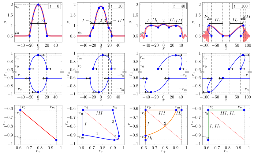
Fig. 1: Behavior of characteristic quantities of the system. Each column corresponds to a given value of $t$, each row to a different type of quantity. The top row displays the light intensity distribution $\rho(x,t)$ plotted as a function of $x$. Both the numerical solution of Eq. (4) (red thick curves) and the analytic dispersionless solution (blue curves) are shown. The initial state is represented in the left panel and corresponds to Eq. (26) with $\rho_{0}=0.5$, $\rho_{m}=2$, $l=20$. The dynamics of the system is governed by Eq. (4) with $\gamma=1$. The middle row displays the (analytic result for) the Riemann invariants $r_{+}(x,t)$ ($r_{+}\in[r_{0},r_{m}]$) and $r_{-}(x,t)$ ($r_{-}\in[-r_{m},-r_{0}]$) plotted as functions of $x$. The set of initial condition corresponds to $r_{0}=0.651$ and $r_{m}=0.955$. Arrows indicate the direction of propagation. In the top and middle row the dashed lines divide space into several regions according to the behavior of the Riemann invariants. The Roman numbers indicate simple-wave regions, the Arabic ones correspond to regions in which both Riemann invariants are position-dependent. The bottom row represents the behavior of Riemann invariants in the hodograph plane. The dotted lines show the boundaries of the domain $[r_{0},r_{m}]\times[-r_{m},-r_{0}]$. Arabic and Roman numbers correspond to the notations of the regions from the top rows of the figure. Here the red curves correspond to $t=0$, the blue curves to $t=10$, the orange curves to $t=40$ and the green curves to $t=100$. The red dotted line represents the diagonal coinciding with the initial curve ${\cal C}$.

This initial density profile is represented in the left panel on the top row of Fig. 1, it is an even function of $x$; generalization to non-symmetric distributions is straightforward. If $l\gg\rho_{m}-\rho_{0}$, then deviations of the exact solution from its hydrodynamic approximation are negligibly small almost everywhere, except in small regions at the boundaries of the bump.

We denote the characteristic values of the Riemann invariant as $r_{0}$ and $r_{m}$ with

$$r_{0}=r_{+}(|x|\geq l,t=0)=\frac{1}{\sqrt{\gamma}}\arctan{\sqrt{\gamma\rho_{0}}},$$ (27a)

$$r_{m}=r_{+}(x=0,t=0)=\frac{1}{\sqrt{\gamma}}\arctan{\sqrt{\gamma\rho_{m}}},$$ (27b)

see the left panel in the middle row of Fig. 1. It is convenient to denote by $\overline{x}(r)$ the positive branch of the reciprocal function of $r_{+}(x,t=0)$:

$$r_{+}(x,0)=\tfrac{1}{2}\int_{0}^{\overline{\rho}}\frac{c(\rho^{\prime})}{\rho^{\prime}}d\rho^{\prime}.$$ (28)

One gets

$$\overline{\rho}(r_{+})=\frac{1}{\gamma}\tan^{2}\left(\sqrt{\gamma}r_{+}\right),$$ (29)

and

$$\overline{x}(r)=l\sqrt{\frac{\rho_{m}-\overline{\rho}(r)}{\rho_{m}-\rho_{0}}}.$$ (30)

For the zero velocity initial profile we consider, Eq. (12) shows that the curve $\mathcal{C}$ which represents the initial condition ($r_{+}(x,0),r_{-}(x,0)$) in the hodograph plane is a segment of the antidiagonal $r_{-}=-r_{+}=-r$. Along it Eqs. (17) with $t=0$ give

$$\left.\frac{\partial W}{\partial r_{-}}\right|_{\mathcal{C}}=\left.\frac{\partial W}{\partial r_{+}}\right|_{\mathcal{C}}=x.$$ (31)

hence $W$ is constant along ${\cal C}$. The value of this constant can be arbitrarily fixed to zero: ${W}(r,-r)=0$, and expressions (23) reduce to

$$U=\frac{x}{2}\,R(r,-r;\xi,\eta),\quad V=-\frac{x}{2}\,R(r,-r;\xi,\eta).$$ (32)

The top row of Fig. 1 shows the light intensity $\rho(x,t)$ plotted as a function of position for different $t$. The middle row represents the corresponding distributions of the Riemann invariants. At a given time, the $x$ axis can be considered as divided into several domains, each requiring a specific treatment. Each domain is characterized by the behavior of the Riemann invariants and is identified in the upper row of Fig. 1. The domains in which both Riemann invariants depend on $x$ are labeled by Arabic numbers and the ones in which only one Riemann invariant depends on $x$ are labeled by Roman numbers. As was noted above, at the initial moment $r_{+}=-r_{-}$, as can be seen, e.g., in the left panel of the middle row of Fig. 1. Then, one of the Riemann invariants begins to move in the positive direction of the $x$ axis, and the other moves in the opposite direction. This behavior initially leads to the configuration represented in the second column of Fig. 1, where two simple-wave regions ($I$ and $III$) and a new region (labeled “2”) have appeared. At later times (i.e., for longer sample lengths) region 2 persists while regions $1$ and $3$ vanish and new simple-wave regions $II_{l}$ and $II_{r}$ appear; this is illustrated in the third columns of Fig. 1. At even larger lengths (right column of Fig. 1), region $2$ also disappears and only simple-wave regions persist: The initial pulse has completely split into two pulses propagating in opposite directions.

It is worth noticing that the wave breaking corresponds to an overlap between different regions which results in a multi-valued solution. If we consider for instance the right propagating pulse, at the wave breaking time $t_{\rm\scriptscriptstyle WB}$, region $III$ starts overlapping with the (unnamed) quiescent region where both Riemann invariants are constants, at the right of the plot. Then these two regions both overlap with region $II_{r}$. These two configurations are respectively illustrated in the columns $t=40$ and $t=100$ of Fig. 1. We will not dwell on this aspect in detail, since a multi-valued solution is nonphysical and, when dispersion is taken into account, it is replaced by a dispersive shock wave (considered in Sec. 4).

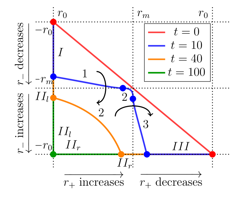
Fig. 2: Distributions of $r_{+}$ and $r_{-}$ in the four-sheeted hodograph plane (see the text). The curves are the unfolded versions of the ones of the bottom row of Fig. 1. The red line corresponds to the input distribution ($t=0$), while other colors correspond to other values of $t$, with the same color code as in the bottom row of Fig. 1. Curved arrows indicate the direction of unfolding of the domain $[r_{0},r_{m}]\times[-r_{m},-r_{0}]$. The whole region above red line is unreachable for the initial distribution which we consider.

The bottom row in Fig. 1 represents the behavior of $r_{+}$ and $r_{-}$ in the hodograph plane. Here, as before, the simple-wave regions are indicated by Roman numerals while the Arabic numerals correspond to regions where both Riemann invariants depend on $x$. In each of the three domains 1, 2, and 3, the solution $W$ of the Euler-Poisson equation has a different expression. In order to describe these three branches, following Ludford Ludford-52 , we introduce several sheets in the characteristic plane by unfolding the domain $[r_{0},r_{m}]\times[-r_{m},-r_{0}]$ into a four times larger region as illustrated in Fig. 2. The potential $W(r_{+},r_{-})$ can now take a different form in each of the regions labeled $1$, $2$, and $3$ in Fig. 2 and still be considered as a single valued. From the relation (22) we can obtain $W(\xi,\eta)$ in regions $1$ and $3$, by computing the right hand side integral along the anti-diagonal ${\cal C}$, between the points $A$ of coordinates $(-\eta,\eta)$ and $B$ of coordinates $(\xi,-\xi)$:

$$\begin{split}W^{(3)}(\xi,\eta)=-W^{(1)}(\xi,\eta)=\int_{-\eta}^{\xi}\overline{x}(r)R(r,-r;\xi,\eta)dr\end{split}$$ (33)

The difference in signs in the above expressions of $W$ comes from the fact that $x=\mp\overline{x}(r)$ depending on if one is in region $1$ or $3$. For the region $2$, using unfolded surfaces (see Fig. 2 and also Ref. ikp-19c ) and upon integrating by parts one obtains

$$\begin{split}W^{(2)}(\xi,\eta)&=\left(RW^{(1)}\right)_{B}+\left(RW^{(3)}\right)_{A}\\ &+\int_{A}^{C}\left.\left(\frac{\partial R}{\partial r_{-}}-aR\right)\right|_{r_{+}=r_{m}}W^{(3)}dr_{-}\\ &-\int_{C}^{B}\left.\left(\frac{\partial R}{\partial r_{+}}-bR\right)\right|_{r_{-}=-r_{m}}W^{(1)}dr_{+},\end{split}$$ (34)

where the coordinates of the relevant points are: $A=(r_{m},\eta)$, $B=(\xi,-r_{m})$ and $C=(r_{m},-r_{m})$.

From the conditions (25) one can find that

$$\begin{split}R(r_{+},\eta;\xi,\eta)=&\sqrt{\frac{c(\xi-\eta)}{c(r_{+}-\eta)}}\exp{\left(\frac{1}{2}\int_{\xi-\eta}^{r_{+}-\eta}\!\!\!\!\frac{dr}{c(r)}\right)},\\ R(\xi,r_{-};\xi,\eta)=&\sqrt{\frac{c(\xi-\eta)}{c(\xi-r_{-})}}\exp{\left(\frac{1}{2}\int_{\xi-\eta}^{\xi-r_{-}}\!\!\!\!\frac{dr}{c(r)}\right)}.\end{split}$$ (35)

These expressions suggest that $R$ can be looked for in the form

$$\begin{split}R(r_{+},r_{-};\xi,\eta)=&\\ \sqrt{\frac{c(\xi-\eta)}{c(r_{+}-r_{-})}}&\exp{\left(\frac{1}{2}\int_{\xi-\eta}^{r_{+}-r_{-}}\!\!\!\!\frac{dr}{c(r)}\right)}F(r_{+},r_{-};\xi,\eta),\end{split}$$ (36)

where $F(r_{+},\eta;\xi,\eta)=F(\xi,r_{-};\xi,\eta)=1$. For small enough $t$, when $\xi$ is close to $r_{m}$ and $\eta$ is close to $-r_{m}$, the integrand functions in Eq. (34) are small by virtue of Eqs. (25); accordingly $F\simeq 1$ in Eq. (36). Such an approximation has been already used in Ref. ikp-19a for discarding the integrated terms in the right-hand side of Eq. (34), and showed good applicability to the situation when $\gamma=0$. Thus, using this approximation, we obtain an approximate expression for the Riemann function (see also Ref. ikp-19c ):

$$R(r_{+},r_{-};\xi,\eta)\simeq\mathscr{R}(r_{+}-r_{-},\xi-\eta),$$ (37)

where

$$\begin{split}\mathscr{R}(r_{1},r_{2})&=\sqrt{\frac{c(r_{2})}{c(r_{1})}}\exp{\left(\frac{1}{2}\int_{r_{2}}^{r_{1}}\!\!\frac{dr}{c(r)}\right)}\\ &=\sqrt{\frac{c(r_{2})\rho(r_{1})}{c(r_{1})\rho(r_{2})}},\end{split}$$ (38)

where $\rho$ is expressed as a function of $r_{1}$ (or $r_{2}$) through Eq. (14). A simple calculation yields

$$\mathscr{R}(r_{1},r_{2})=\sqrt{\frac{\sin\left(\frac{\sqrt{\gamma}}{2}r_{1}\right)\cos^{3}\left(\frac{\sqrt{\gamma}}{2}r_{2}\right)}{\sin\left(\frac{\sqrt{\gamma}}{2}r_{2}\right)\cos^{3}\left(\frac{\sqrt{\gamma}}{2}r_{1}\right)}}.$$ (39)

We can thus adapt expressions (33) for $W$ in regions $1$ and $3$

$$\begin{split}W^{(1)}&(r_{+},r_{-})=-W^{(3)}(r_{+},r_{-})=\\ &-\int_{-r_{-}}^{r_{+}}\!\!\!\overline{x}(r)\mathscr{R}(2r,r_{+}-r_{-})dr,\\ \end{split}$$ (40)

whereas expression (34) in region $2$ now reads

$$\begin{split}W^{(2)}(r_{+},r_{-})=&\mathscr{R}(r_{m}-r_{-},r_{+}-r_{-})W^{(3)}(r_{m},r_{-})\\ +&\mathscr{R}(r_{+}+r_{m},r_{+}-r_{-})W^{(1)}(r_{+},-r_{m}).\end{split}$$ (41)

In expressions (40) and (41) we have made, with respect to Eqs. (33) and (34), the replacements $\xi\rightarrow r_{+}$, $\eta\rightarrow r_{-}$ so that these expressions can be used in Eqs. (19) and then (17). The knowledge of the expression of $W$ is the regions where both Riemann invariants vary (regions 1,2 and 3) makes it possible to compute $r_{\pm}(x,t)$ in these regions, as detailed in Ref. ikp-19c . The density and velocity profiles are then obtained from Eqs. (12) and (14).

3.3 Simple wave solution

In the simple-wave regions, where one of the Riemann invariants is constant, the hodograph transform does not apply. In such a region however, the solution of the problem is relatively easy. For instance, during the initial stages of evolution, when the regions $I$ and $III$ still exist, we can solve the problem by means of the method of characteristics. We look for a solution in the form

$$\begin{split}x-v_{+}(r_{+},-r_{0})t&=h^{III}(r_{+}),\qquad\text{for region $III$},\\ x-v_{-}(r_{0},r_{-})t&=h^{I}(r_{-}),\qquad\text{for region $I$}.\end{split}$$ (42)

where the functions $h^{III}$ and $h^{I}$ are determined by boundary conditions: the simple wave solution should match with the solution in regions where both Riemann invariants vary at the interface between the two regions ($III$ and 3 or $I$ and 1). This yields from Eqs. (17)

$$\begin{split}x-v_{+}(r_{+},-r_{0})t=\frac{\partial W^{(3)}(r_{+},-r_{0})}{\partial r_{+}},\end{split}$$ (43)

for the simple-wave region $III$, and

$$\begin{split}x-v_{-}(r_{0},r_{-})t=\frac{\partial W^{(1)}(r_{0},r_{-})}{\partial r_{-}},\end{split}$$ (44)

for region $I$.

After a certain time, two new simple-wave regions appear, which are denoted as $II_{l}$ and $II_{r}$ in Fig. 1). Similarly, we get

$$\begin{split}x-v_{+}(r_{+},-r_{0})t=\frac{\partial W^{(2)}(r_{+},-r_{0})}{\partial r_{+}},\end{split}$$ (45)

for region $II_{r}$, and for region $II_{l}$:

$$\begin{split}x-v_{-}(r_{0},r_{-})t=\frac{\partial W^{(2)}(r_{0},r_{-})}{\partial r_{-}}.\end{split}$$ (46)

From the results presented in Secs. 3.2 and 3.3 we obtain a complete description of the dispersionless stage of evolution of the system. The top row of Fig. 1 displays a comparison of the results of this approach with the numerical solution of Eq. (4). There is a very good agreement up to the wave breaking moment. For subsequent time ($t>t_{\rm\scriptscriptstyle WB}$) the dispersionless evolution becomes multi-valued in some regions of space (indicating a breakdown of the approach and the occurrence of a DSW), but remains accurate in others which we denote as “dispersionless regions” below. Note that these regions can be precisely defined only after the extension of the DSW has been properly determined. This question is addressed in the following section.

4 Dispersive shock waves

The basic mathematical approach for the description of DSWs is based on the Whitham modulation theory Whitham-65 ; Whitham-74 . This treatment relies on the large difference between the fast oscillations within the wave and the slow evolution of its envelope. It results in the so-called Whitham modulation equations which constitute a very complex system of nonlinear first order differential equations. Whitham’s great achievement was to be able to transform such a system — in the very important and universal case of the Korteweg-de Vries (KdV) equation — into a diagonal (Riemann) form analogous to the system (10). This achievement enabled Gurevich and Pitaevskii gp-73 to successfully apply the Whitham theory to the description of DSWs dynamics for the KdV equation in a system experiencing simple wave breaking. It became clear later that the possibility to diagonalize the system of Whitham equations is closely related with the complete integrability of the KdV equation, and Whitham theory was extended to many completely integrable equations, as described, for example, in the reviews DubrovinNovikov-93 and Kamchatnov-97 .

However, a large number of equations are not completely integrable — among which Eq. (4) — and require the development of a more general theory for describing DSWs. An important success in this direction was obtained by El who developed in Ref. El-05 a method that made it possible to find the main parameters of a DSW arising from the evolution of an initial discontinuity. Recently, it was shown in Ref. Kamchatnov-19 that El’s method can be generalized to a substantial class of initial conditions, such as simple waves, for which the limiting expressions for the characteristic velocities of the Whitham system at the edges of the DSW are known from general considerations as being equal to either the group velocity of the wave at the boundary with a smooth solution, or the soliton velocity at the same boundary. This information, together with the knowledge of the smooth solution in the dispersionless regions, is enough to find the law of motion of the corresponding edge of the DSW for an arbitrary initial profile. We will use the methods of Ref. Kamchatnov-19 to find the dynamics of the edges of the DSW in our case.

The specific dispersive properties of the system under consideration enter into the general theory in the form of Whitham’s “number of waves” conservation law Whitham-65 ; Whitham-74

$$\frac{\partial k}{\partial t}+\frac{\partial\omega(k)}{\partial x}=0,$$ (47)

where $k=2\pi/L$ and $\omega=kV$ are the wave vector and the angular frequency of a single phase nonlinear wave, $L$ being its wavelength and $V$ its phase velocity. Because of the large difference between the scales characterizing the envelope and those characterizing the oscillations within the wave, Eq. (47) is valid along the whole DSW. At the small amplitude edge of the DSW the function $\omega(k)$ becomes the linear dispersion relation $\omega_{\rm lin}(k)$ in the system. In our case, this dispersion law is obtained by linearizing equations (6) around the uniform state $\rho=\rho_{0}$, $u=u_{0}$ (we keep here a nonzero value of $u_{0}$ for future convenience); that is, we write $\rho(x,t)=\rho_{0}+\rho^{\prime}(x,t)$ and $u(x,t)=u_{0}+u^{\prime}(x,t)$, where $|\rho^{\prime}|\ll\rho_{0}$ and $|u^{\prime}|\ll u_{0}$. A plane wave expansion of $\rho^{\prime}$ and $u^{\prime}$ immediately yields

$$\omega_{\rm lin}(k)\equiv ku_{0}\pm k\sqrt{\frac{\rho_{0}}{(1+\gamma\rho_{0})^{2}}+\frac{k^{2}}{4}}.$$ (48)

Thus, if one can calculate the wave number at the small-amplitude edge of the DSW, one obtains the speed of propagation of this edge as being equal to the corresponding group velocity $v_{g}(k)=d\omega_{\rm lin}/dk$.

Unfortunately, this approach cannot be applied straightforwardly at the soliton edge of a DSW. In spite of that, El showed El-05 that under some additional assumptions one can obtain from Eq. (47) an ordinary differential equation relating the physical variables along the characteristic of Whitham equations at the soliton edge of the DSW. The idea is based on the following remark: At the tails of a soliton, the density profile has an exponential form $\propto\exp(-\widetilde{k}|x-V_{s}t|)$, where $V_{s}$ is the speed of the soliton. Of course a soliton propagates at the same velocity as its tails, which, being a small perturbations of the background, obey the linear dispersion law $\omega=\omega_{\rm lin}(k)$. Hence, as was noticed by Stokes stokes (see also Sec. 252 in lamb ), we arrive at the statement that the soliton velocity $V_{s}$ is related to its “inverse half-width” $\widetilde{k}$ by the formula

$$V_{s}={\widetilde{\omega}(\widetilde{k})}/{\widetilde{k}},\quad\mbox{where}\quad\widetilde{\omega}(\widetilde{k})\equiv-i\omega_{\rm lin}(i\widetilde{k}).$$ (49)

However, the “solitonic counterpart”

$$\frac{\partial\widetilde{k}}{\partial t}+\frac{\partial\widetilde{\omega}(\widetilde{k})}{\partial x}=0$$ (50)

of Eq. (47) does not apply in all possible DSW configurations, even at the soliton edge. Interestingly, it does apply for a step-like type of initial conditions, and El used this property to determine the inverse half-width and velocity of a soliton edge, using a procedure similar to the one employed at the small amplitude edge. As a result, a number of interesting problems were successfully considered by this method, see, e.g., Refs. egkkk-07 ; ElGrimshaw-06 ; ElGrimshaw-09 ; EslerPearce-11 ; Hoefer-14 ; CKP-16 ; HEK-17 ; AnMarchant-18 .

To go beyond the initial step-like type of problems, one has to use some additional information about the properties of the Whitham modulation equations at the edges of DSWs (see Refs. Kamchatnov-19 ; IvanovKamchatnov-2019 ). For integrable equations, it is known that the “soliton number of waves conservation law” (50) is valid in the case where the DSW is triggered by a simple wave breaking Kamchatnov-19 . Therefore, it is natural to assume that Eq. (50) also applies for non-integrable equations in situations where the pulse considered propagates into a uniform and stationary medium and experiences a simple wave breaking.

We can consider that the smooth solution of the dispersionless equations is known from the approach presented in Sec. 3. At the boundary between the dispersionless simple wave region and the DSW, Eqs. (47) and (50) reduce to ordinary differential equations which can be extrapolated to the whole DSW. Their solution, with known boundary condition at both edges, yields the wave number $k$ and the inverse half-width of solitons $\widetilde{k}$ at the boundary with the smooth part of the pulse. Consequently, the corresponding group velocity or the soliton velocity at a DSW edge can be expressed in terms of the parameters of the smooth solution at its boundary with a DSW. These velocities can be considered as the characteristic velocities of the limiting Whitham equations at this edge, which makes it possible to represent these equations in the form of first order partial differential equations after a hodograph transformation. The compatibility condition for this partial differential equation with a smooth dispersionless solution gives the law of motion of this DSW edge. If the soliton solution of the nonlinear equation at hand is known, then the knowledge of its velocity makes it possible to also determine its amplitude at the boundary of the DSW. In this paper, we shall apply this method to study the evolution of initial simple-wave pulses in the generalized NLS equation (4).

We suppose that in the whole region of the DSW, one has

$$\begin{split}r_{-}&=\frac{u}{2}-\frac{1}{\sqrt{\gamma}}\arctan{\sqrt{\gamma\rho}}\\ &=-\frac{1}{\sqrt{\gamma}}\arctan{\sqrt{\gamma\rho_{0}}}=-r_{0}=\rm{cst}.\end{split}$$ (51)

This occurs for instance in the DSW formed at the right of the right propagating bump issued from the initial condition (26) — for which the behavior of the dispersionless Riemann invariants is sketched in Fig. 1 — and also in the model cases studied in Secs. 4.1.1 and 4.2 below.

Equation (10b) is satisfied identically by virtue of our assumption (51). Also, since $r_{-}$ is constant, $r_{+}$ and $u$ can be considered as functions of $\rho$ only [see Eqs. (12) and (13)]:

$$\begin{split}u(\rho)&=\frac{2}{\sqrt{\gamma}}\left(\arctan{\sqrt{\gamma\rho}}-\arctan{\sqrt{\gamma\rho_{0}}}\right),\\ r_{+}(\rho)&=\frac{1}{\sqrt{\gamma}}\left(2\arctan{\sqrt{\gamma\rho}}-\arctan{\sqrt{\gamma\rho_{0}}}\right),\end{split}$$ (52)

and Eq. (10a) for $r_{+}$ thus takes the form

$$\frac{\partial\rho}{\partial t}+(u(\rho)+c(\rho))\frac{\partial\rho}{\partial x}=0,$$ (53)

where the expression of the local sound velocity is given in (8). The general solution (17a) of Eq. (10a) here specializes to

$$x-(u(\rho)+c(\rho))t=w_{+}(r_{+}(\rho),-r_{0}).$$ (54)

All the relevant characteristic quantities of the DSW formed after the wave breaking of such a pulse can be considered to be functions of $\rho$ only. We can thus write the right propagating soliton dispersion law (49) in the form

$$\begin{split}\widetilde{\omega}(\widetilde{k})&=\widetilde{k}\left[u(\rho)+\sqrt{c^{2}(\rho)-\tfrac{1}{4}\widetilde{k}^{2}}\right]\\ &=\widetilde{k}\left[u(\rho)+c(\rho)\widetilde{\alpha}(\rho)\right],\end{split}$$ (55)

where

$$\widetilde{\alpha}(\rho)=\sqrt{1-\frac{\widetilde{k}^{2}}{4\,c^{2}(\rho)}}.$$ (56)

We then have

$$\widetilde{k}(\rho)=2\,c(\rho)\,\sqrt{1-\widetilde{\alpha}^{2}(\rho)},$$ (57)

where $\widetilde{\alpha}(\rho)$ is yet an unknown function.

As implied by El’s method, along the soliton edge of the DSW one considers that $r_{-}$ is also a constant, and that, at all time, the quantities $u$, $c$, $r_{+}$, $\widetilde{k}$, $\widetilde{\alpha}$ and $\widetilde{\omega}$ can be considered as functions of $\rho$ only. Then the solitonic “number of wave conservation” (50) yields, with account of (53):

$$\frac{d\,\widetilde{\omega}}{d\rho}=[u(\rho)+c(\rho)]\frac{d\,\widetilde{k}}{d\rho}.$$ (58)

Substitution of (55) and (57) into this equation yields an ordinary differential equation for $\widetilde{\alpha}(\rho)$,

$$\frac{d\widetilde{\alpha}}{d\rho}=-\frac{(1+\widetilde{\alpha})(1+3\gamma\rho+2\widetilde{\alpha}(1-\gamma\rho))}{2\rho(1+\gamma\rho)(1+2\widetilde{\alpha})},$$ (59)

which should be solved with the boundary condition appropriate to the situation considered (see below).

The same method is employed for studying the motion of the small amplitude edge of the DSW. This edge propagates at the linear group velocity, and for determining the relevant wave-vector, we rewrite equation (48) in the form

$$\omega_{\rm lin}(k)=k\left[u(\rho)+c(\rho)\alpha(\rho)\right],$$ (60)

that is

$$\alpha(\rho)=\sqrt{1+\frac{k^{2}}{4\,c^{2}(\rho)}},$$ (61)

and

$$k(\rho)=2\,c(\rho)\sqrt{\alpha^{2}(\rho)-1}.$$ (62)

A simple calculation leads to the following differential equation

$$\frac{d\alpha}{d\rho}=-\frac{(1+\alpha)(1+3\gamma\rho+2\alpha(1-\gamma\rho))}{2\rho(1+\gamma\rho)(1+2\alpha)},$$ (63)

which actually coincides with the equation (59). Now we “extrapolate” this equation across the entire DSW an determine the wave-vector as the value of $k(\rho)$ at the density of the small amplitude edge. The appropriate boundary condition for solving (63) is fixed at the solitonic edge, and depends on the configuration under study (see below).

4.1 Positive pulse

In all this section we consider an initial condition with a region of increased light intensity over a stationary uniform background.

4.1.1 Constant Riemann invariant $r_{-}$

As a first illustration of the method we consider an initial condition for which the Riemann invariant $r_{-}$ has the constant value $-r_{0}$ for all $x$. We shall start with a pulse with the following initial intensity distribution:

$$\overline{\rho}(x)=\begin{cases}\rho_{0}+\widetilde{\rho}(x)&\mbox{if}\quad x<0,\\ \rho_{0}&\mbox{if}\quad x\geq 0,\end{cases}$$ (64)

where $\widetilde{\rho}(x)$ is a decreasing function of $x$ with a vertical tangent at $x\to 0^{-}$, see Fig. 3(a).

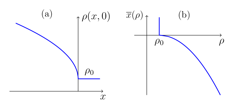
Fig. 3: (a) Initial profile $\overline{\rho}(x)$ of a monotonous positive pulse. (b) Inverse function $\overline{x}(\rho)$.

From (9) one then obtains $u(x,0)=\overline{u}(x)$ with

$$\overline{u}(x)=\frac{2}{\sqrt{\gamma}}\arctan\sqrt{\gamma\overline{\rho}(x)}-2\,r_{0}\;.$$ (65)

This non-standard type of initial condition is of interest because it enables to test the theory just presented in a particularly simple setting in which (i) the evolution of the non-dispersive part of the system is that of a simple wave, i.e., one can replace $w_{+}$ in the right hand side of Eq. (54) by $\overline{x}(\rho)$, where $\overline{x}(\rho)$ is the function inverse to the initial distribution of the intensity $\overline{\rho}(x)$ (see Fig. 3(b)), (ii) the wave breaking occurs instantaneously, at the front edge of the pulse. This wave breaking is followed by the formation of a DSW with a small-amplitude wave at its front edge and with solitons at its trailing edge, at the boundary with the smooth part of the pulse [described by the equation (54)]. Therefore, we can find the law of motion of the rear solitons edge of the DSW by the method of Ref. Kamchatnov-19 .

Eq. (59) should be solved with the boundary condition $\widetilde{\alpha}(\rho_{0})=1$, that is, the soliton inverse half-width vanishes together with its amplitude at the small-amplitude edge.

When the function $\widetilde{\alpha}(\rho)$ is known, the velocity of the front edge can be represented as the soliton velocity

$$V_{s}=\frac{\widetilde{\omega}}{\widetilde{k}}=u(\rho_{s})+c(\rho_{s})\widetilde{\alpha}(\rho_{s}),$$ (66)

where $\rho_{s}$ is the density at the solitonic edge of the DSW. We notice again that $V_{s}$ is the characteristic velocity of the Whitham modulation equations at the soliton edge. The system being nonintegrable, the corresponding Whitham equation is not known, but its limiting form at the solitonic edge can be written explicitly: along this boundary one has $dx_{s}-V_{s}dt=0$, where $x_{s}(t)$ is the position of the solitonic edge at time $t$ and $\rho_{s}=\rho(x_{s}(t),t)$. It is convenient to re-parametrize all the quantities in term of $\rho_{s}$: $x(\rho_{s})$ and $t(\rho_{s})$. This leads to

$$\frac{\partial x_{s}}{\partial\rho_{s}}-V_{s}(\rho_{s})\frac{\partial t}{\partial\rho_{s}}=0.$$ (67)

This equation should be compatible with Eq. (53) at the solitonic boundary between the DSW and the dispersionless region gives, with account of (54). Here, the specific initial condition we have chosen (with $r_{-}(x,0)=\rm{cst}$) simplifies the problem because one has $w_{+}(r_{+}(\rho),-r_{0})=\bar{x}(\rho)$. The compatibility equation then reads

$$\frac{\sqrt{\rho_{s}}}{1+\gamma\rho_{s}}(1-\widetilde{\alpha})\frac{dt}{d\rho_{s}}+\frac{3+\gamma\rho_{s}}{2\sqrt{\rho_{s}}(1+\gamma\rho_{s})^{2}}t=-\frac{d\overline{x}(\rho_{s})}{d\rho_{s}}.$$ (68)

One sees from Fig. (3) that for the initial condition we consider, the wave breaking occurs instantly at $t=0$, with $\rho_{s}=\rho_{0}$. Hence Eq. (68) should be integrated with the initial condition $t(\rho_{0})=0$. The corresponding solution reads

$$t(\rho_{s})=\int_{\rho_{0}}^{\rho_{s}}\frac{(1+\gamma\rho)\overline{x}^{\prime}(\rho)G(\rho_{s},\rho)}{\sqrt{\rho}(\widetilde{\alpha}(\rho)-1)}d\rho,$$ (69)

where $\overline{x}^{\prime}=d\overline{x}/d\rho$ and

$$G(\rho_{s},\rho)=\exp{\left(\int_{\rho}^{\rho_{s}}\frac{3+\gamma\rho^{\prime}}{2\rho^{\prime}(1+\gamma\rho^{\prime})(\widetilde{\alpha}(\rho^{\prime})-1)}d\rho^{\prime}\right)}.$$ (70)

Consequently,

$$x_{s}(\rho_{s})=\left[u(\rho_{s})+c(\rho_{s})\right]t(\rho_{s})+\overline{x}(\rho_{s}),$$ (71)

where $u(\rho)$ and $c(\rho)$ are given by Eqs. (52) and (8), respectively.

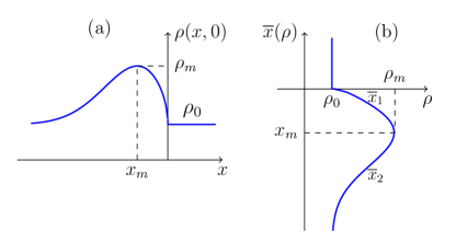
Fig. 4: (a) Initial profile $\overline{\rho}(x)$ of a non-monotonous positive pulse. (b) The inverse function $\overline{x}(\rho)$ is represented by two branches $\overline{x}_{1}(\rho)$ and $\overline{x}_{2}(\rho)$. Here $x_{m}$ is the point where $\rho$ reaches its maximal value $\rho_{m}$.

As a generalisation of the model initial profile represented in Fig. 3, we now consider the case where the initial distribution $\overline{\rho}(x)$ is non monotonous, with a single maximum. This amounts to assume that $\widetilde{\rho}$ in (64) has a maximum $\rho_{m}$ at $x=x_{m}<0$, tends to 0 fast enough as $x\to-\infty$, with still a vertical tangent at $x\to 0^{-}$, see Fig. 4(a). This last condition means that we suppose again for convenience that the wave breaks at the moment $t=0$. The reciprocal function of $\overline{\rho}(x)$ becomes now two-valued and we denote its two branches as $\overline{x}_{1}(\rho)$ and $\overline{x}_{2}(\rho)$, see Fig. 4(b). In an initial stage of development of the DSW, the formulas obtained previously for a monotonous initial condition straightforwardly apply. This occurs when the maximum of the smooth part of the profile issued from the initial distribution has not yet penetrated the DSW. In this case the soliton edge propagates along the branch $\overline{x}_{1}(\rho)$ and one should just use this function instead of $\overline{x}(\rho)$ in Eqs. (69) and (71). A second stage begins when the maximum of the smooth part of the profile reaches the DSW. In this case one can show that Eqs. (69) and (71) are modified to

$$t(\rho_{s}) =\int_{\rho_{0}}^{\rho_{m}}\frac{(1+\gamma\rho)\overline{x}_{1}^{\prime}(\rho)G(\rho_{s},\rho)}{\sqrt{\rho}(\widetilde{\alpha}(\rho)-1)}d\rho$$

$$\quad+\int_{\rho_{m}}^{\rho_{s}}\frac{(1+\gamma\rho)\overline{x}_{2}^{\prime}(\rho)G(\rho_{s},\rho)}{\sqrt{\rho}(\widetilde{\alpha}(\rho)-1)}d\rho,$$ (72a)

$$x_{s}(\rho_{s}) =\left[u(\rho_{s})+c(\rho_{s})\right]t(\rho_{s})+\overline{x}_{2}(\rho_{s}).$$ (72b)

To determine the position of the small-amplitude edge we solve Eq. (63) with the boundary condition

$$\alpha(\rho_{m})=1,$$ (73)

which corresponds to the moment at which the soliton edge reaches the maximal point of the initial distribution. The corresponding solution $\alpha(\rho)$ yields the spectrum (62) of all possible wave numbers $k(\rho)$, with $\rho$ ranging from $\rho_{0}$ to $\rho_{m}$. The maximal value of the group velocity $d\omega_{\rm lin}/dk$ is reached at $\rho=\rho_{0}$ and it provides the asymptotic value of the velocity of the small amplitude edge:

$$\frac{dx_{r}}{dt}=\left.\frac{d\omega_{\rm lin}}{dk}\right|_{\rho=\rho_{0}}=\frac{\sqrt{\rho_{0}}}{1+\gamma\rho_{0}}\frac{2\alpha^{2}(\rho_{0})-1}{\alpha(\rho_{0})}.$$ (74)

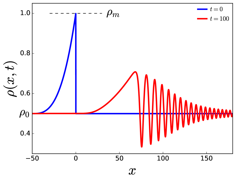
Fig. 5: Blue solid curve: simple-wave initial condition (75) with $\rho_{0}=0.5$, $\rho_{m}=1$ and $x_{0}=50$. Red solid curve: resulting dispersive shock wave computed by numerically solving Eq. (4) with $\gamma=1$.

As an illustration of the accuracy of the method, we now compare the theoretical results with those of a numerical solution of the generalized NLS equation (4) for the non-monotonous initial intensity distribution

$$\overline{\rho}(x)=\begin{cases}\rho_{0}+(\rho_{m}-\rho_{0})\left(\frac{x}{x_{0}}+1\right)^{3}\;\mbox{if}\;x\in[-x_{0},0],\\ \rho_{0}\quad\mbox{elsewhere},\end{cases}$$ (75)

see the blue curve in Fig. 5. The typical form of the DSW generated by such a pulse is represented in the same figure by a red curve. For the particular initial profile (75) the branch $\overline{x}_{1}(\rho)$ shrinks to zero, the first term in the right hand side of (72a) cancels and we need take into account only the contribution of the second branch, given by the expression

$$\overline{x}_{2}(\rho\geq\rho_{0})=x_{0}\left(\frac{\rho-\rho_{0}}{\rho_{m}-\rho_{0}}\right)^{1/3}-x_{0}.$$ (76)

For the numerical simulation, we took instead of the idealized profile (75) the numerical initial condition:

$$\overline{\rho}(x)=\rho_{0}+(\rho_{m}-\rho_{0})\left(1+x/x_{0}\right)^{3}\frac{1-\tanh(x/w)}{2}\;,$$ (77)

with $w=1$, $x_{0}=50$, $\rho_{0}=0.5$ and $\rho_{m}=1$. Equation (77) yields a maximum value of $\overline{\rho}$ which is not exactly equal to $\rho_{m}=1$, but to $\overline{\rho}_{\rm max}=0.9362$.

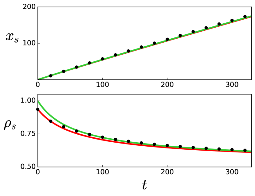
Fig. 6: Position $x_{s}(t)$ and density $\rho_{s}(t)$ of the solitonic edge of the DSW induced by the initial profile (75) and (65). The black dots are obtained by numerical integration of Eq. (4). The colored solid lines are obtained from the analytic formulas (72). In each plot the green theoretical solid line is obtained by taking $\rho_{m}=1$ and the red one by taking $\rho_{m}=0.9362$ (see the text).

Eqs. (72) give the parametric dependence of the soliton edge position $x_{s}(t)$ and density $\rho_{s}(t)$, which are represented in Fig. 6 by continuous colored curves. For the analytic determination of $\rho_{s}(t)$ and $x_{s}(t)$ we used in Eqs. (72) two possible values of $\rho_{m}$: 1 (green curve in Fig. 6) and 0.9362 (red curve). As one can see, there is no much difference, and the theoretical results both agree well with the numerical simulations (black dots). Of course, the results at short time for $\rho_{s}$ are better when one takes the initial $\rho_{m}=0.9362$, but this has little incidence at large time, and the results for $x_{s}$ almost do not depend on the choice $\rho_{m}=1$ or 0.9362.

For our initial parameters, the analytic formula (74) gives the asymptotic propagation velocity of the right small-amplitude edge of the DSW: $dx_{r}/dt=1.11$. The numerical value of the velocity is $1.12$ for our choice of initial condition, an agreement which should be considered as very good since the position of the small-amplitude edge is not easily determined, as is clear from Fig. 5, and we evaluate it by means of an approximate extrapolation of the envelopes of the wave at this edge.

4.1.2 The parabolic initial condition (26)

We now consider the initial density profile (26) with $u(x,0)=0$; that is, an initial state which is not of simple wave type, and for which the formulas of the previous Sec. 4.1.1 are not directly applicable. In this case, the wave breaking of the right propagating part of the pulse occurs in region $III$, where $r_{-}$ is constant and equal to $-r_{0}$ at $\rho_{s}(t_{\rm\scriptscriptstyle WB})=\rho(x_{s}(t_{\rm\scriptscriptstyle WB}),t_{\rm\scriptscriptstyle WB})=\rho_{0}$. Hence Eq. (59) should be integrated with the boundary condition $\widetilde{\alpha}(\rho_{0})=1$. In a first stage of its development, the DSW matches the dispersionless profile described by Eq. (43) where $W^{(3)}(r_{+},r_{-})$ is given by Eq. (40) and $\overline{x}(r)$ by (30).

In the region of interest for us $r_{-}=-r_{0}$, so all quantities in Eq. (43) depend on $r_{+}$ only. Differentiation with respect to $r_{+}$ yields, at the solitonic edge where $dx_{s}=V_{s}dt$:

$$(V_{s}-v_{+})\frac{dt}{dr_{+}}-\frac{dv_{+}}{dr_{+}}\,t=\frac{\partial^{2}W^{(3)}}{\partial r_{+}^{2}}\;,$$ (78)

where all quantities are evaluated at $r_{s}=r_{+}(x_{s}(t),t)$ and $r_{-}=-r_{0}$. It follows from (13) that $dr_{s}=c(\rho_{s})d\rho_{s}/\rho_{s}$, yielding

$$\frac{dv_{+}}{dr_{+}}=1+\frac{\rho_{s}}{c(\rho_{s})}\,\frac{dc}{d\rho_{s}}=\frac{3+\gamma\rho_{s}}{2(1+\gamma\rho_{s})}.$$ (79)

For explicitly evaluating the right hand side of Eq. (78) it is convenient to write $\mathscr{R}(r_{1},r_{2})=f(r_{1})/f(r_{2})$ in Eq. (40) [see expressions (38) and (39)] which leads to

$$\frac{\partial W^{(3)}}{\partial r_{+}}=-\frac{f^{\prime}(r_{+}-r_{-})}{f(r_{+}-r_{-})}\,W^{(3)}+\frac{\overline{x}(r_{+})f(2r_{+})}{f(r_{+}-r_{-})}\;,$$ (80)

and

$$\begin{split}&\frac{\partial^{2}W^{(3)}}{\partial r_{+}^{2}}=\left[2\,\frac{f^{\prime 2}(r_{+}-r_{-})}{f^{2}(r_{+}-r_{-})}-\frac{f^{\prime\prime}(r_{+}-r_{-})}{f(r_{+}-r_{-})}\right]W^{(3)}\\ &-2\,\overline{x}(r_{+})\,\frac{f^{\prime}(r_{+}-r_{-})f(2r_{+})-f(r_{+}-r_{-})f^{\prime}(2r_{+})}{f^{2}(r_{+}-r_{-})}\\ &+\frac{d\overline{x}}{dr_{+}}\frac{f(2r_{+})}{f(r_{+}-r_{-})}\;.\end{split}$$ (81)

At the wave-breaking time $t_{\rm\scriptscriptstyle WB}$ one has $r_{s}=r_{0}$; Eqs. (40), (80) and (81) then directly yield $W^{(3)}=0$, $\partial W^{(3)}/\partial r_{+}=\overline{x}(r_{0})=l$ and [using Eqs. (30) and (29)]

$$\frac{\partial^{2}W^{(3)}}{\partial r_{+}^{2}}=\left.\frac{d\overline{x}}{dr}\right|_{r=r_{0}}=-l\,\frac{(1+\gamma\rho_{0})\sqrt{\rho_{0}}}{\rho_{m}-\rho_{0}}.$$ (82)

At the wave breaking $V_{s}=v_{+}$ [$\widetilde{\alpha}(\rho_{0})=1$ in (66)] and Eq. (78) thus yields

$$t_{\rm\scriptscriptstyle WB}=\frac{l}{\rho_{m}-\rho_{0}}\frac{2\sqrt{\rho_{0}}(1+\gamma\rho_{0})^{2}}{3+\gamma\rho_{0}}.$$ (83)

This result is in agreement with the findings of Ref. ikp-19c and reduces to the one obtained in Ref. ikp-19a for the nonlinear Schrödinger equation in the limit $\gamma=0$. For the example considered in Fig. 1, expression (83) gives $t_{\rm\scriptscriptstyle WB}=12.12$.

For times larger than $t_{\rm\scriptscriptstyle WB}$ one should solve Eq. (78) using the generic form (81) of its right hand side. It is convenient to multiply this equation by $\rho_{s}/c(\rho_{s})(dr_{s}/d\rho_{s})=1$, which yields

$$\rho_{s}\left(\widetilde{\alpha}(\rho_{s})-1\right)\frac{dt}{d\rho_{s}}-\frac{3+\gamma\rho_{s}}{2(1+\gamma\rho_{s})}\,t=\frac{\partial^{2}W^{(3)}(r_{s},-r_{0})}{\partial r_{s}^{2}}.$$ (84)

The solution reads

$$t(\rho_{s})=\int_{\rho_{0}}^{\rho_{s}}\frac{\partial^{2}W^{(3)}}{\partial r_{+}^{2}}\frac{G(\rho_{s},\rho)}{\rho(\widetilde{\alpha}(\rho)-1)}\,d\rho,$$ (85)

where the expression of $G$ is given in (70) and $r_{+}$ and $\overline{x}$ should be computed as functions of $\rho$ via Eqs. (52), (29) and (30). Once $t(\rho_{s})$ is known, $x_{s}(\rho_{s})$ is determined from Eq. (43). One can check that expression (85) yields the correct result (83) for $t_{\rm\scriptscriptstyle WB}$: When $\rho$ is close to $\rho_{0}$ one gets from Eq. (70) and (59) (with $\widetilde{\alpha}(\rho_{0})=1$):

$$G(\rho_{s},\rho)\simeq\left(\frac{\rho-\rho_{0}}{\rho_{s}-\rho_{0}}\right)^{3/2}\;.$$ (86)

Inserting this expression back into (85) one obtains

$$t(\rho_{0})=-\frac{2(1+\gamma\rho_{0})}{3+\gamma\rho_{0}}\left(\frac{\partial^{2}W^{(3)}}{\partial r_{+}^{2}}\right)_{r_{+}=r_{0}}\;.$$ (87)

That is, as expected, $t(\rho_{0})=t_{\rm\scriptscriptstyle WB}$, where $t_{\rm\scriptscriptstyle WB}$ is given by Eq. (83).

The solution (85) is acceptable only up to a time which we denote as $t_{\rm 2|3}$ at which $r_{s}=r_{m}$, i.e., $\rho_{s}$ reaches a maximum which we denote as $\rho_{\scriptscriptstyle\rm M}$ where [see Eq. (14)]

$$\rho_{\scriptscriptstyle\rm M}=\gamma^{-1}\tan^{2}[\sqrt{\gamma}(r_{m}+r_{0})/2]\;.$$ (88)

At times larger than $t_{2|3}$ the region $III$ disappears and the DSW is in contact with region $II_{r}$ of the dispersionless profile in which Eq. (45) applies. Instead of (84) one should thus solve

$$\rho_{s}\left(\widetilde{\alpha}(\rho_{s})-1\right)\frac{dt}{d\rho_{s}}-\frac{3+\gamma\rho_{s}}{2(1+\gamma\rho_{s})}\,t=\frac{\partial^{2}W^{(2)}(r_{s},-r_{0})}{\partial r_{s}^{2}},$$ (89)

with the initial condition $t(\rho_{\scriptscriptstyle\rm M})=t_{2|3}$. $W^{(2)}$ in the above equation is given by Eq. (41) which can be cast in the form

$$\begin{split}W^{(2)}(r_{+},r_{-})=\frac{1}{f(r_{+}-r_{-})}&\Big{[}\int_{-r_{-}}^{r_{m}}\overline{x}(r)f(2r)dr\\ &+\int_{r_{+}}^{r_{m}}\overline{x}(r)f(2r)dr\Big{]}.\end{split}$$ (90)

This yields

$$\frac{\partial W^{(2)}}{\partial r_{+}}=-\frac{f^{\prime}(r_{+}-r_{-})}{f(r_{+}-r_{-})}\,W^{(2)}-\frac{\overline{x}(r_{+})f(2r_{+})}{f(r_{+}-r_{-})},$$ (91)

and

$$\begin{split}&\frac{\partial^{2}W^{(2)}}{\partial r_{+}^{2}}=\left[2\,\frac{f^{\prime 2}(r_{+}-r_{-})}{f^{2}(r_{+}-r_{-})}-\frac{f^{\prime\prime}(r_{+}-r_{-})}{f(r_{+}-r_{-})}\right]W^{(2)}\\ &+2\,\overline{x}(r_{+})\,\frac{f^{\prime}(r_{+}-r_{-})f(2r_{+})-f(r_{+}-r_{-})f^{\prime}(2r_{+})}{f^{2}(r_{+}-r_{-})}\\ &-\frac{d\overline{x}}{dr_{+}}\frac{f(2r_{+})}{f(r_{+}-r_{-})}.\end{split}$$ (92)

The solution of (89) reads

$$t(\rho_{s})=t_{2|3}+\int_{\rho_{\scriptscriptstyle\rm M}}^{\rho_{s}}\frac{\partial^{2}W^{(2)}}{\partial r_{+}^{2}}\frac{G(\rho_{s},\rho)}{\rho(\widetilde{\alpha}(\rho)-1)}\,d\rho.$$ (93)

Once $t(\rho_{s})$ is determined from (93) $x_{s}(\rho_{s})$ is obtained from (45). Formulas (85), (43), (93) and (45) give parametric expressions of $\rho_{s}(t)$ and $x_{s}(t)$ for all $t\geq t_{\rm\scriptscriptstyle WB}$.

We note here that in the limit $\gamma\to 0$, the solution of Eq. (59) reads $\widetilde{\alpha}=-1+2\sqrt{\rho_{0}/\rho}$ which, from (66), yields $V_{s}=\sqrt{\rho_{s}}=\tfrac{1}{2}(r_{s}-r_{-})$, in agreement with the findings of Ref. ikp-19a . Also in this limit, one gets the exact expression $G(\rho_{s},\rho)=(\sqrt{\rho}-\sqrt{\rho_{0}})^{3/2}(\sqrt{\rho_{s}}-\sqrt{\rho_{0}})^{-3/2}$ and formulas (85) and (93) reduce to the equivalent ones derived for the NLS equation in Ref. ikp-19a .

In the generic case $\gamma\neq 0$, the results for $x_{s}(t)$ and $\rho_{s}(t)$ corresponding to the parameters of Fig. 1 are compared in Fig. 7 with the values extracted from the numerical solution of Eq. (4) (with $\gamma=1$).

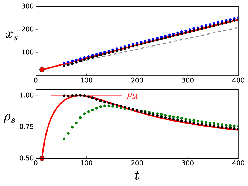
Fig. 7: Position $x_{s}(t)$ and density $\rho_{s}(t)$ of the solitonic edge of the DSW induced by the initial profile (26) with $\rho_{0}=0.5$, $\rho_{m}=2$ and $l=20$. The continuous red curves are the theoretical results. The big red dots locate the wave breaking time $t_{\rm\scriptscriptstyle WB}=12.12$, position $x_{s}(t_{\rm\scriptscriptstyle WB})=25.71$ and intensity $\rho(x_{s}(t_{\rm\scriptscriptstyle WB}),t_{\rm\scriptscriptstyle WB})=\rho_{0}$. The dotted curves are extracted from numerical simulations (see the text). The dashed gray line in the upper panel corresponds to a soliton edge which would propagate at the background sound velocity. The horizontal red line in the lower panel marks the position of the maximum $\rho_{\scriptscriptstyle\rm M}$ as given by Eq. (88).

The position $x_{s}$ of the solitonic edge is easily determined from the numerical simulation: it is located between the maximum of the smooth part of the intensity and the following zero of $\rho-\rho_{0}$ (respectively black and blues dots in the upper panel of the figure). The intensity $\rho_{s}$ of the solitonic edge is more difficult to extract from the numerical simulations in the present situation that in the case studied in Fig. 6. At times close to the theoretical wave-breaking time, one cannot exactly decide from the numerical intensity profile if the oscillations at the boundary of the right propagating edge of the region of increased intensity are linear disturbances (due to dispersive effects) or correspond to the birth of a DSW. It is only after a certain amount of time that the oscillations become clearly nonlinear. Even then, the precise location of the intensity of the solitonic edge is not easily determined: it is comprised between the maximum intensity of the smooth part of the spectrum and the following maximum intensity (respectively black and green dots in the lower panel of Fig. 7). The green dots initially yield a clear under estimate of $\rho_{s}$, and, on the contrary, when the dispersive shock if fully developed, they indicate a too large value. This is due to the fact that, at large time, the amplitude of the oscillations in the vicinity of the soliton edge increase within the DSW.

We note also that expression (88) gives a simple and accurate prediction for the maximum of $\rho_{s}$ ($\rho_{\scriptscriptstyle\rm M}=1$ in the case considered in Fig. 7). At times large compare to the time $t_{2|3}$ at which this maximum is reached, one can approximately evaluate the behavior of $\rho_{s}$ and $x_{s}$ as follows: The integrands in Eqs. (85) and (93) are of the form $(\rho_{s}-\rho_{0})^{-3/2}F^{(i)}(\rho_{s},\rho)$ where $F$ is a non singular function [with $i=2$ for Eq. (85) and $i=3$ for Eq. (93)]. Since at large time $\rho_{s}$ tends to $\rho_{0}$, formula (93) can be approximated by

$$t(\rho_{s})\simeq\frac{{\cal A}}{(\rho_{s}-\rho_{0})^{3/2}},$$ (94)

where

$${\cal A}=\int_{\rho_{0}}^{\rho_{\scriptscriptstyle\rm M}}\left(F^{(3)}(\rho_{0},\rho)-F^{(2)}(\rho_{0},\rho)\right)d\rho.$$ (95)

From there it follows that, at large $t$, $\rho_{s}$ tends to $\rho_{0}$ as $t^{-2/3}$ and $x_{s}$ exceeds $c(\rho_{0})t$ by a factor of order $t^{1/3}$. The fact that the soliton edge propagates at a velocity higher that the speed of sound is illustrated in Fig. 7 by the difference between $x_{s}(t)$ and the gray dashed line of equation $x=x_{s}(t_{\rm\scriptscriptstyle WB})+c(\rho_{0})(t-t_{\rm\scriptscriptstyle WB})$.

A final remark is in order here. When $\rho_{m}$ gets large compared with $\rho_{0}$, $\widetilde{\alpha}(\rho_{s})$—solution of (59)—may become negative. For instance, when $\gamma=0$ this occurs for $\rho_{m}\geq 4\,\rho_{0}$. As noticed in Ref. egkkk-07 , this is linked to the occurrence within the DSW of a vacuum point El1995 at which the density cancels. In this case, one should use another branch in the dispersion relations (48) and (55), but once this modification is performed, the approach remains perfectly valid and accurate.

When $\gamma>0$, a more serious problem occurs at larger values of $\rho_{m}$, when $\widetilde{\alpha}(\rho_{s})$ reaches $-\tfrac{1}{2}$. A rough estimate based on the regime $\gamma\ll 1$ indicates that this occurs starting from $\rho_{m}\approx 16\,\rho_{0}$. In this case the theoretical approach leads to singularities [see, e.g., Eq. (59)] whereas the numerical simulations do not indicate a drastic change of behavior in the dynamics of the DSW. This points to a probable failure of the Gurevich-Meshcherkin-El approach, however the study of this problem is beyond the scope of the present work and we confine ourselves to a regime of initial parameters for which $\widetilde{\alpha}(\rho_{s})$ remains larger than $-\tfrac{1}{2}$ and the theory is applicable.

4.2 Negative pulse

In this section we consider an initial condition with a region where the density is depleted with respect to that of the background. For simplicity we only consider the case where, as in Sec. 4.1.1, the initial Riemann invariant $r_{-}(x,0)$ is constant and equal to $-r_{0}$ for all $x$.

Let us first consider a monotonous initial pulse

$$\rho(x,0)=\begin{cases}\rho_{0}&\mbox{if}\quad x<0,\\ \rho_{0}-\widetilde{\rho}(x)&\mbox{if}\quad x\geq 0.\end{cases}$$ (96)

This initial condition is sketched in Fig. 8.

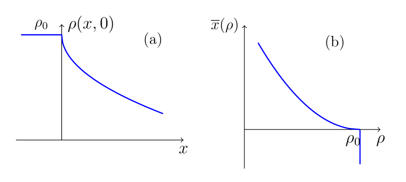
Fig. 8: (a) Initial profile $\overline{\rho}(x)$ of a monotonous negative pulse. (b) Inverse function $\overline{x}(\rho)$.

The small-amplitude edge propagates with the group velocity

$$V_{r}(\rho_{r})=\frac{d\omega}{dk}=u(\rho_{r})+\frac{\sqrt{\rho_{r}}}{1+\gamma\rho_{r}}\frac{2\alpha^{2}(\rho_{r})-1}{\alpha(\rho_{r})},$$ (97)

where $\rho_{r}(t)$ is the density of the small amplitude edge. Following a reasoning analogous to the one already employed in Sec. 4.1.1 for the solitonic edge, we parameterize all relevant quantities at the small amplitude edge in term of $\rho_{r}$. This leads to the following differential equation

$$\frac{\sqrt{\rho_{r}}}{1+\gamma\rho_{r}}\frac{2\alpha^{2}-\alpha-1}{\alpha}\frac{dt}{d\rho_{r}}-\frac{3+\gamma\rho_{r}}{2\sqrt{\rho_{r}}(1+\gamma\rho_{r})^{2}}t=\frac{d\overline{x}(\rho_{r})}{d\rho_{r}},$$ (98)

which should be solved with the initial condition $\rho_{r}=\rho_{0}$ at $t=0$. The solution reads

$$t(\rho_{r})=\int_{\rho_{0}}^{\rho_{r}}{\frac{\alpha(\rho)(1+\gamma\rho)\overline{x}^{\prime}(\rho)G(\rho_{r},\rho)}{\sqrt{\rho}(\alpha(\rho)-1)(1+2\alpha(\rho))}}d\rho,$$ (99)

where $\overline{x}^{\prime}(\rho)=d\overline{x}/d\rho$ and

$$\begin{split}G&(\rho_{r},\rho)=\\ &\exp{\left(\int_{\rho}^{\rho_{r}}\!\!\frac{\alpha(\rho^{\prime})(3+\gamma\rho^{\prime})\,d\rho^{\prime}}{2\rho^{\prime}(1+\gamma\rho^{\prime})(\alpha(\rho^{\prime})-1)(1+2\alpha(\rho^{\prime}))}\right)}.\end{split}$$ (100)

Consequently, the position $x_{r}$ of the small amplitude edge is given by

$$x_{r}(\rho_{r})=\left[u(\rho_{r})+c(\rho_{r})\right]t(\rho_{r})+\overline{x}(\rho_{r}),$$ (101)

where $u(\rho)$ is given by Eq. (52). Formulas (99) and (101) determine, in a parametric form, the coordinates $x_{r}(t)$ and $\rho_{r}(t)$ of the small-amplitude edge.

In the case of a non-monotonous negative pulse, such as the one represented in Fig. 9, the approach has to be modified in a manner similar to that exposed in Sec. 4.1.1 for the non-monotonous profile displayed in Fig. 4. We do not write down the corresponding formulas for not overloading the paper with almost identical expressions. We only indicate that $\rho_{m}$ denotes now the minimal value of the density in the initial distribution.

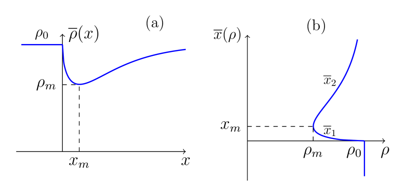
Fig. 9: (a) Initial profile $\overline{\rho}(x)$ of a non-monotonous negative pulse. (b) The inverse function $\overline{x}(\rho)$ is represented by two branches $\overline{x}_{1}(\rho)$ and $\overline{x}_{2}(\rho)$. Here $x_{m}$ is the point where $\rho$ takes its minimal value $\rho_{m}$.

For numerically testing our approach we consider a non-monotonous initial profile of the form

$$\overline{\rho}(x)=\begin{cases}\rho_{0}-(\rho_{m}-\rho_{0})\left(\frac{x}{x_{0}}-1\right)^{3}\;\mbox{if}\;x\in[0,x_{0}],\\ \rho_{0}\quad\mbox{elsewhere},\end{cases}$$ (102)

see the blue curve in Fig. 10. In this case one has $\overline{x}_{1}(\rho)=0$ and

$$\overline{x}_{2}(\rho\leq\rho_{0})=x_{0}-x_{0}\left(\frac{\rho_{0}-\rho}{\rho_{0}-\rho_{m}}\right)^{1/3}.$$ (103)

The initial velocity distribution $u(x,0)$ is determined from (102) by imposing that $r_{-}(x,0)=-r_{0}$. The typical wave pattern for the light evolved from such a pulse is shown in Fig. 10.

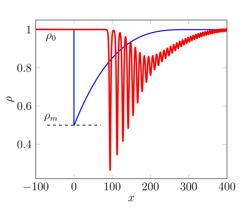
Fig. 10: Density profile $\rho(x,t=300)$ (red solid curve), which results from the time evolution of the simple-wave initial condition (102) with $\rho_{0}=1$, $\rho_{m}=0.5$ and $x_{0}=300$ (blue solid curve).

The motion of the right, small amplitude edge is determined as previously explained. Eq. (63) should be solved with the initial condition $\alpha(\rho_{m})=1$. Then, in the non-monotonous case we consider here, Eq. (98) should be solved with an initial condition different from the one used in the case of the initial profile (96). The appropriate initial value is here $\rho_{r}=\rho_{m}$ at $t=0$. As a result, the lower boundary of the integration region in (99) should be changed from $\rho_{0}$ to $\rho_{m}$.

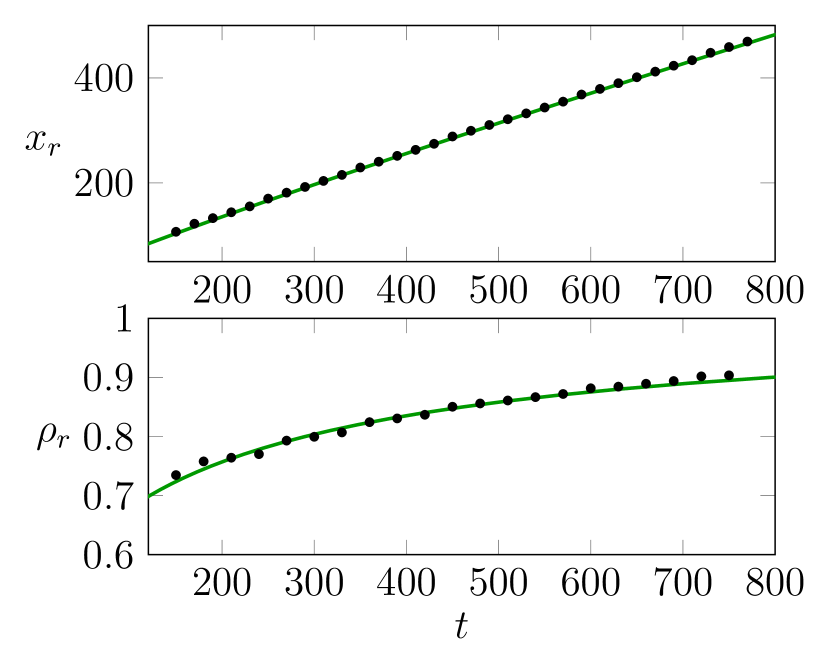
Fig. 11: Coordinate $x_{r}(t)$ and density $\rho_{r}(t)$ of the small-amplitude edge of the DSW induced by the initial profile (102). The black dots are obtained by numerical integration of Eq. (4). The green solid lines are obtained from the analytic solution, i.e., from Eqs. (99) and (101).

The theoretical results compare very well with the one extracted from the numerical simulations, as illustrated in Fig. 11. Note that the determination of the small amplitude edge of the numerical DSW is a delicate task, which is simplified if the DSW contains a large number of oscillations. This is the reason why we had to chose here an initial profile of extension larger than the one considered in the previous section 4.1.1 ($x_{0}=300$ instead of 50). Note however that the case considered here presents an advantage compared to the similar one considered in Sec. 4.1.1: the motion of the small-amplitude edge is less dependent of the precise characteristics of $\overline{\rho}(x)$ at its extremum than the motion of the solitonic edge. As a result, we need not discuss here the precise numerical implementation of the idealized discontinuous profile (102), contrarily with what has been done in Sec. 4.1.1.

At asymptotically large time the velocity of the trailing soliton generated from a localized pulse is determined from the knowledge of $\widetilde{\alpha}(\rho_{0})$, where $\widetilde{\alpha}(\rho)$ is the solution of equation (59) with the boundary condition $\widetilde{\alpha}(\rho_{m})=1$. Within this approximation, the asymptotic velocity of the soliton edge reads

$$V_{s}(t\to\infty)=\frac{\sqrt{\rho_{0}}}{1+\gamma\rho_{0}}\widetilde{\alpha}(\rho_{0}).$$ (104)

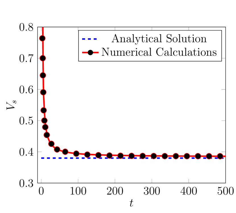
Fig. 12: Black dots: numerically determined velocity $V_{s}(t)$ of the soliton edge. The initial conditions are specified in Eq. (102) with $\rho_{0}=1$, $\rho_{m}=0.7$ and $x_{0}=300$ (blue). Continuous red line: fit of the numerical data by the formula: $V_{s}(t)=V_{s}^{\rm num}+\sum_{i=1}^{6}a_{i}t^{-i}$. One obtains $V_{s}^{\rm num}=0.39$, in good agreement with the theoretical prediction from Eq. (104): $V_{s}(t\to\infty)=0.37$ (blue dashed line).

The comparison of the analytic prediction (104) with our numerical simulations is not difficult because the soliton edge is easily identified in the numerical density profiles, and, indeed, a leading soliton is easily located at this edge of the numerically determined DSW. As we see in Fig. 12, its velocity tends at large $t$ to a constant value. In this figure, the numerical result is fitted with the empirical formula $V_{s}(t)=V_{s}^{\rm num}+\sum_{i=1}^{6}a_{i}t^{-i}$, where $V_{s}^{\rm num}$ and $a_{i}$ are fitting parameters. The trend is in excellent agreement with the prediction (104) since one obtains $V_{s}^{\rm num}=0.39$ whereas from (104) one expects $V_{s}(t\to\infty)=0.37$.

5 Conclusion

In this work we have presented a theoretical study of the dynamics of spreading of a pulse of increased (or decreased) intensity propagating over a uniform background. The initial non-dispersive stage of evolution is described by means of Riemann’s method, the result of which compares very well with numerical simulations. After the wave breaking time, we have studied the behavior of the resulting dispersive shock wave at its edges, by mean of the modification of El’s method presented in Ref. Kamchatnov-19 . Here also the results compare very well with the ones of numerical simulations.

Our work represents a comprehensive theoretical description of the spreading, of the wave breaking and of the subsequent formation of a dispersive shock in a realistic setting for a system described by a nonintegrable nonlinear equation. In particular, our approach yields a simple analytic expression for the wave-breaking time, even in situations where the initial density and velocity profiles do not reduce to a simple wave configuration. Also, in view of future experimental studies, we have devoted a special attention to the determination of the position and intensity of the solitonic edge of the DSW issued from the spreading of a region of increased light intensity.

- (1) Z. Dutton, M. Budde, C. Slowe, and L. V. Hau, Observation of Quantum Shock Waves Created with Ultra- Compressed Slow Light Pulses in a Bose-Einstein Condensate, Science 293, 663 (2001).
- (2) T. P. Simula, P. Engels, I. Coddington, V. Schweikhard, E. A. Cornell, and R. J. Ballagh, Observations on Sound Propagation in Rapidly Rotating Bose-Einstein Condensate, Phys. Rev. Lett. 94, 080404 (2005).
- (3) M. A. Hoefer, M. J. Ablowitz, I. Coddington, E. A. Cornell, P. Engels, and V. Schweikhard, Phys. Rev. A 74, 023623 (2006).
- (4) N. Ghofraniha, C. Conti, G. Ruocco, and S. Trillo, Shocks in nonlocal media, Phys. Rev. Lett. 99, 043903 (2007).
- (5) N. Ghofraniha, S. Gentilini, V. Folli, E. DelRe, and C. Conti, Shock waves in disordered media, Phys. Rev. Lett. 109, 243902 (2012).
- (6) G. Xu, A. Mussot, A. Kudlinski, S. Trillo, F. Copie, and M. Conforti, Shock wave generation triggered by a weak background in optical fibers, Optics Letters 41, 11 (2016).
- (7) G. Xu, M. Conforti, A. Kudlinski, A. Mussot, and S. Trillo, Dispersive dam-break flow of a photon fluid, Phys. Rev. Lett. 118, 254101 (2017).
- (8) G. Marcucci, M. Braidotti, S. Gentilini, and C. Conti, Time asymmetric quantum mechanics and shock waves: Exploring the irreversibility in nonlinear optics, Ann. Phys. (Berlin) 529, 1600349 (2017).
- (9) J. Nuño, C. Finot, G. Xu, G. Millot, M. Erkintalo, and J. Fatome, Vectorial dispersive shock waves in optical fibers, Commun. Phys. 2, 138 (2019).
- (10) M. G. Forest, C.-J. Rosenberg, and O. C. Wright III, On the exact solution for smooth pulses of the defocusing nonlinear Schrödinger modulation equations prior to breaking, Nonlinearity 22, 2287 (2009)
- (11) S. K. Ivanov and A. M. Kamchatnov, Collision of rarefaction waves in Bose-Einstein condensates Phys. Rev. A 99, 013609 (2019).
- (12) M. Isoard, A. M. Kamchatnov, and N. Pavloff, Wave breaking and formation of dispersive shock waves in a defocusing nonlinear optical material, Phys. Rev. A 99, 053819 (2019).
- (13) M. Isoard, A. M. Kamchatnov, and N. Pavloff, Short-distance propagation of nonlinear optical pulses, in Compte-rendus de la 22 rencontre du Non Linéaire, Eds. E. Falcon, M. Lefranc, F. Pétrélis, C.-T. Pham, (Non-Linéaire Publications, Saint-Étienne du Rouvray, 2019).
- (14) M. Isoard, A. M. Kamchatnov, and N. Pavloff, Dispersionless evolution of inviscid nonlinear pulses, EPL 129, 64003 (2020).
- (15) G. B. Whitham, Non-linear dispersive waves, Proc. R. Soc. London, Ser. A 283, 238 (1965).
- (16) G. B. Whitham, Linear and Nonlinear Waves, (Wiley Interscience, New York, 1974).
- (17) A. M. Kamchatnov, Nonlinear Periodic Waves and Their Modulations—An Introductory Course, (World Scientific, Singapore, 2000).
- (18) G. A. El and M. A. Hoefer, Dispersive shock waves and modulation theory, Physica D 333, 11 (2016).
- (19) M. G. Forest and J. E. Lee, Geometry and modulation theory for periodic nonlinear Schrödinger equation, in Oscillation Theory, Computation, and Methods of Compensated Compactness, Eds. C. Dafermos et al., IMA Volumes on Mathematics and its Applications 2, p. 35 (Springer, N.Y., 1986).
- (20) M. V. Pavlov, Nonlinear Schrödinger equation and the Bogolyubov-Whitham method of averaging, Teor. Mat. Fiz. 71, 351 (1987) [Theoret. Math. Phys. 71, 584 (1987)].
- (21) A. V. Gurevich and L. P. Pitaevskii, Nonstationary structure of a collisionless shock wave, Zh. Eksp. Teor. Fiz. 65, 590 (1973) [Sov. Phys. JETP 38, 291 (1974)].
- (22) A. V. Gurevich and A. L. Krylov, Dissipationless shock waves in media with positive dispersion, Zh. Eksp. Teor. Fiz. 92, 1684 (1987) [Sov. Phys. JETP 65, 944 (1987)].
- (23) G. El, V. Geogjaev, A. Gurevich, and A. Krylov, Decay of an initial discontinuity in the defocusing NLS hydrodynamics, Physica D 87, 186 (1995).
- (24) G. A. El, A. L. Krylov, General solution of the Cauchy problem for the defocusing NLS equation in the Whitham limit, Phys. Lett. A 203, 77 (1995).
- (25) R. Z. Sagdeev, Cooperative Phenomena and Shock Waves in Collisionless Plasmas, in Reviews of Plasma Physics, Ed. M. A. Leontovich, Vol. 4, p. 23, (Consultants Bureau, New York, 1966).
- (26) G. Couton, H. Mailotte, and M. Chauvet, Self-formation of multiple spatial photovoltaic solitons, J. Opt. B: Quantum Semiclassical Opt. 6, S223 (2004).
- (27) W. Wan, S. Jia, and J. W. Fleischer, Dispersive superfluid-like shock waves in nonlinear optics, Nat. Phys. 3, 46 (2007).
- (28) A. V. Gurevich and A. P. Meshcherkin, Expanding self-similar discontinuities and shock waves in dispersive hydrodynamics, Zh. Eksp. Teor. Fiz. 87, 1277-1291 (1984) [Sov. Phys. JETP 60, 732-740 (1984)].
- (29) L. D. Landau and E. M. Lifshitz, Fluid Mechanics, (Pergamon, Oxford, 1987).
- (30) G. A. El, Resolution of a shock in hyperbolic systems modified by weak dispersion, Chaos 15, 037103 (2005).
- (31) G. A. El, R. H. J. Grimshaw, N. F. Smyth, Unsteady undular bores in fully nonlinear shallow-water theory, Phys. Fluids 18, 027104 (2006).
- (32) G. A. El, A. Gammal, E. G. Khamis, R. A. Kraenkel, and A. M. Kamchatnov, Theory of optical dispersive shock waves in photorefractive media, Phys. Rev. A 76, 053813 (2007).
- (33) G. A. El, R. H. J. Grimshaw, N. F. Smyth, Transcritical shallow-water flow past topography: finite-amplitude theory, J. Fluid Mech. 640, 187 (2009).
- (34) J. G. Esler, J. D. Pearce, Dispersive dam-break and lock-exchange flows in a two-layer fluid, J. Fluid Mech. 667, 555 (2011).
- (35) M. A. Hoefer, Shock waves in dispersive Eulerian fluids, J. Nonlinear Sci. 24, 525 (2014).
- (36) T. Congy, A. M. Kamchatnov, and N. Pavloff, Dispersive hydrodynamics of nonlinear polarization waves in two component Bose-Einstein condensates, SciPost Phys. 1, 006 (2016).
- (37) M. A. Hoefer, G. A. El, A. M. Kamchatnov, Oblique spatial dispersive shock waves in nonlinear Schrödinger flows, SIAM J. Appl. Math. 77, 1352 (2017).
- (38) X. An, T. R. Marchant and N. F. Smyth, Dispersive shock waves governed by the Whitham equation and their stability, Proc. Roy. Soc. London A 474, 20180278 (2018).
- (39) A. M. Kamchatnov, Dispersive shock wave theory for nonintegrable equations, Phys. Rev. E 99, 012203 (2019).
- (40) S. K. Ivanov and A. M. Kamchatnov, Evolution of wave pulses in fully nonlinear shallow-water theory, Physics of Fluids 31, 057102 (2019).
- (41) T. Bienaimé, private communication.
- (42) L. D. Landau and E. M. Lifshitz, Electrodynamics of Continupous Media, (Pergamon, Oxford, 1984).
- (43) J.L. Coutaz and M. Kull, Saturation of the nonlinear index of refraction in semiconductor-doped glass, J. Opt. Soc. Am. B 8, 95 (1991).
- (44) Y. S. Kivshar and G. P. Agrawal, Optical Solitons, From Fibers to Photonic Crystals (Academic Press, San Diego, 2003).
- (45) R. W. Boyd, Nonlinear Optics (Academic Press, San Diego, 1992).
- (46) Y. Wang and M. Saffman, Experimental study of nonlinear focusing in a magneto-optical trap using a Z-scan technique, Phys. Rev. A 70, 013801 (2004).
- (47) N. Šantić, A. Fusaro, S. Salem, J. Garnier, A. Picozzi, and R. Kaiser, Nonequilibrium Precondensation of Classical Waves in Two Dimensions Propagating through Atomic Vapors, Phys. Rev. Lett. 120, 055301 (2018).
- (48) Q. Fontaine, T. Bienaimé, S. Pigeon, E. Giacobino, A. Bramati, and Q. Glorieux, Observation of the Bogoliubov Dispersion in a Fluid of Light, Phys. Rev. Lett. 121, 183604 (2018).
- (49) S. A. Akhmanov, A. P. Sukhorukov, R. V. Khokhlov, Self-focusing and diffraction of light in a Nonlinear medium, Usp. Fiz. Nauk. 93, 19 (1967) [Sov. Phys. Usp. 10, 609 (1968)].
- (50) A. Sommerfeld, Partial Differential Equations in Physics (Academic Press, N. Y., 1949).
- (51) R. Courant and D. Hilbert, Methods of Mathematical Physics, Vol. II (Interscience Publishers, N. Y., 1962).
- (52) G. S. S. Ludford, On an extension of Riemann’s method of integration, with applications to one-dimensional gas dynamics, Proc. Cambridge Philos. Soc. 48, 499 (1952).
- (53) B. A. Dubrovin and S. P. Novikov, Hydrodynamics of Soliton Lattices, Sov. Sci. Rev. Sect. C, Math. Phys. Rev. 9, 1 (1993).
- (54) A. M. Kamchatnov, New approach to periodic solutions of integrable equations and nonlinear theory of modulational instability, Phys. Rep. 286, 199 (1997).
- (55) G. G. Stokes, The Outskirts of the Solitary Wave, in Mathematical and Physical Papers, vol. V, p. 163 (UP, Cambridge, 1905).
- (56) H. Lamb, Hydrodynamics, (UP, Campridge, 1994).
- (57) G. A. El, V. V. Geogjaev, A. V. Gurevich, and A. L. Krylov, Decay of an initial discontinuity in the defocusing NLS hydrodynamics, Physica D 87, 186 (1995).