Dynamics of Atomic Steps on GaN (0001) during Vapor Phase Epitaxy

Abstract

Images of the morphology of GaN (0001) surfaces often show half-unit-cell-height steps separating a sequence of terraces having alternating large and small widths. This can be explained by the $\alpha\beta\alpha\beta$ stacking sequence of the wurtzite crystal structure, which results in steps with alternating $A$ and $B$ edge structures for the lowest energy step azimuths, i.e. steps normal to $[01\overline{1}0]$ type directions. Predicted differences in the adatom attachment kinetics at $A$ and $B$ steps would lead to alternating $\alpha$ and $\beta$ terrace widths. However, because of the difficulty of experimentally identifying which step is $A$ or $B$, it has not been possible to determine the absolute difference in their behavior, e.g. which step has higher adatom attachment rate constants. Here we show that surface X-ray scattering can measure the fraction of $\alpha$ and $\beta$ terraces, and thus unambiguously differentiate the growth dynamics of $A$ and $B$ steps. We first present calculations of the intensity profiles of GaN crystal truncation rods (CTRs) that demonstrate a marked dependence on the $\alpha$ terrace fraction $f_{\alpha}$. We then present surface X-ray scattering measurements performed in situ during homoepitaxial growth on (0001) GaN by vapor phase epitaxy. By analyzing the shapes of the $(10\overline{1}L)$ and $(01\overline{1}L)$ CTRs, we determine that the steady-state $f_{\alpha}$ increases at higher growth rate, indicating that attachment rate constants are higher at $A$ steps than at $B$ steps. We also observe the dynamics of $f_{\alpha}$ after growth conditions are changed. The results are analyzed using a Burton-Cabrera-Frank model for a surface with alternating step types, to extract values for the kinetic parameters of $A$ and $B$ steps. These are compared with predictions for GaN (0001).

I Introduction

The atomic-scale mechanisms of crystal growth are often described within the framework of Burton-Cabrera-Frank (BCF) theory Burton et al. (1951); Jeong and Williams (1999); Woodruff (2015), in which atoms are added to the growing crystal surface by preferential attachment at the steps forming the edges of each exposed atomic layer, or terrace. The motion of the steps during growth defines the classical homoepitaxial crystal growth modes of 1-dimensional step flow, 2-dimensional island nucleation and coalescence, or 3-dimensional roughening Tsao (1993). The BCF model was originally developed for crystals with simple symmetries, with step heights of a full unit cell and step properties that are identical from step to step, for a fixed step direction (in-plane azimuth). However, when the space group of the crystal includes screw axes or glide planes, the growth behavior of steps on surfaces perpendicular to one of these symmetry elements can have fundamentally different characteristics van Enckevort and Bennema (2004). In this case, each succeeding terrace has the same atomic termination, but a different in-plane orientation. These terraces are separated by fractional-unit-cell-height steps. Even for a fixed step azimuth the step structures and properties can vary from step to step. A well-studied example is the Si (001) surface, which is normal to a $4_{2}$ screw axis in the diamond cubic structure. Because the surface reconstructs strongly and reveals the orientation of each terrace, the two types of steps can be clearly identified Tromp et al. (1985).

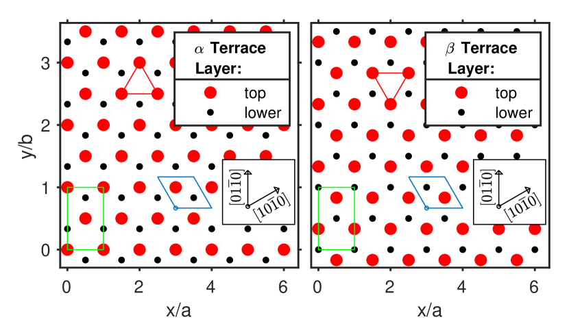
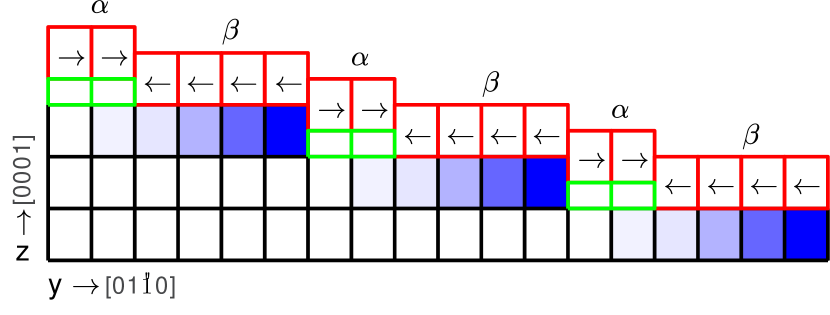
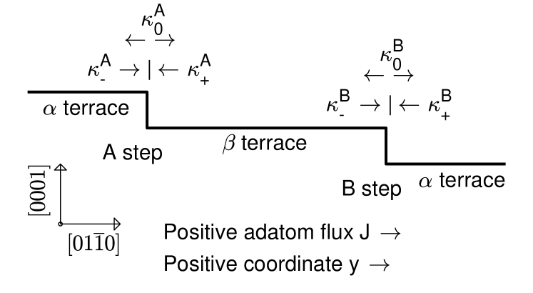
A more subtle and widespread version of this effect occurs on the basal-plane $\{0001\}$-type surfaces of crystals having hexagonal close-packed (HCP) or related structures, which are normal to a $6_{3}$ screw axis. The close-packed layers in HCP crystals have 3-fold symmetry alternating between $180^{\circ}$-rotated orientations from layer to layer, as shown by the $\alpha$ and $\beta$ terrace structures in Fig. 1. The $\alpha\beta\alpha\beta$ stacking sequence typically results in half-unit-cell-height steps on vicinal surfaces. Often the lowest energy steps are normal to $[01\overline{1}0]$-type directions. The alternating structures of these steps are conventionally labelled $A$ and $B$ Xie et al. (1999); Giesen (2001) as shown on Fig. 2. When the in-plane azimuth of an $A$ step changes by $60^{\circ}$, e.g. from $[01\overline{1}0]$ to $[10\overline{1}0]$, its structure changes to $B$, and vice versa. Differences in the dynamics of adatom attachment at $A$ and $B$ steps have strong effects on the surface morphology produced during growth.

Figure 1: Structure of $\alpha$ and $\beta$ terraces of the (0001) surface of an HCP-type crystal, e.g. the Ga sites in wurtzite-structure GaN. Red triangle of top-layer sites around $6_{3}$ screw axis shows difference between alternating $\alpha$ and $\beta$ layers. Blue rhombus shows conventional HCP unit cell; green rectangle shows orthohexagonal unit cell. Axes give coordinates in terms of orthohexagonal lattice parameters $a$ and $b=\sqrt{3}a$.

Figure 2: Terrace and step structure of vicinal (0001) surface of an HCP-type crystal. Circles show in-plane positions of top-layer atoms on each terrace, with color indicating height. Orthohexagonal lattice parameters are $a$, $b$, and $c$. Steps of height $c/2$ typically have lowest edge energy when they are normal to $[01\overline{1}0]$, $[10\overline{1}0]$, or $[1\overline{1}00]$. Steps of a given azimuth have alternating structures, $A$ and $B$. The step structure changes from $A$ to $B$ or $B$ to $A$ when they change azimuth by $60^{\circ}$.

Figure 3: AFM height image of GaN (0001) surface typical of films grown on sapphire substrates by OMVPE, showing regions of alternating step spacings and interlacing at corners where step azimuth changes by $\sim 60^{\circ}$. Step heights are c/2 (2.6 Å).

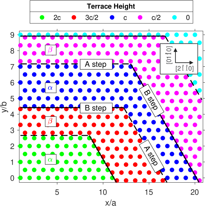
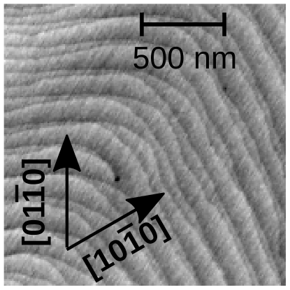
Images of $\{0001\}$ surfaces showing the alternating nature of the steps have been obtained for several HCP-related systems, including SiC Verma (1951); Sunagawa and Bennema (1979); van der Hoek et al. (1982), GaN Xie et al. (1999); Heying et al. (1999); S Vézian et al. (2001); Zauner et al. (2002); Xie et al. (2006); Krukowski et al. (2007); Zheng et al. (2008); Turski et al. (2013); Lin et al. (2013), AlN Pristovsek et al. (2017), and ZnO Chen et al. (2002). As shown in Fig. 3, such images typically indicate a tendency for local pairing of steps (i.e. alternating step spacings), and an “interlaced” structure in which the step pairs switch partners at corners where the step azimuth changes by $60^{\circ}$. In some cases of MBE-grown GaN Xie et al. (1999); S Vézian et al. (2001); Turski et al. (2013), every other step takes on a zigzag morphology, so that all steps are made of segments of only one type, $A$ or $B$. Similar alternating straight and crenellated steps have been observed in OMVPE of AlN Pristovsek et al. (2017). Observations of triangular islands Xie et al. (1999, 2006); Zheng et al. (2008) indicate that one step may grow faster, leaving behind island shapes terminated by the slower growing step. All of these features are consistent with predictions that $A$ and $B$ steps can have significantly different energies and/or attachment kinetics Xie et al. (1999, 2006); Turski et al. (2013); Załuska-Kotur et al. (2011, 2010); Xu et al. (2017); Chugh and Ranganathan (2017a); Akiyama et al. (2020a, b). In particular, different attachment kinetics at $A$ and $B$ steps can produce a tendency to step pairing during growth and thus to different local fractions of $\alpha$ and $\beta$ terraces. In limiting cases, the $\alpha$ terrace fraction $f_{\alpha}$ can approach zero or unity, when pairs of half-unit-cell-height steps join to form full-unit-cell-height steps. However, in contrast to Si (001), for $\{0001\}$ surfaces of HCP-related systems it has been difficult to distinguish experimentally the terrace orientation, and thus to determine whether a given set of steps is of $A$ or $B$ type.

The dynamic properties of $A$ and $B$ steps on GaN (0001) have been predicted in several publications. A seminal study Xie et al. (1999) of MBE growth of GaN posited a higher tendency for adatom attachment at $A$ steps than at $B$ steps, giving faster $A$ steps for a given supersaturation. The support for this result is based on an argument regarding the difference in dangling bonds between $A$ and $B$ steps, and a comparison with experimental results on GaAs (111) Avery et al. (1997); Jo et al. (2012). Face-centered cubic (FCC) materials such as GaAs have $A$ and $B$ type steps on (111) surfaces that do not alternate between successive terraces and thus can be distinguished by their orientation Giesen (2001). In contrast, subsequent theoretical studies of GaN (0001) have consistently predicted that $A$ steps have smaller adatom attachment coefficients than $B$ steps. Kinetic Monte Carlo (KMC) studies of GaN (0001) growth under organo-metallic vapor phase epitaxy (OMVPE) conditions found step pairing Załuska-Kotur et al. (2011) driven by faster kinetics at $B$ steps than $A$ steps Załuska-Kotur et al. (2010). A KMC study of growth on an HCP lattice Xu et al. (2017) found a much lower Ehrlich-Schwoebel (ES) barrier at $B$ steps than at $A$ steps, when only nearest-neighbor jumps are allowed. A recent KMC study of GaN (0001) growth under MBE conditions Chugh and Ranganathan (2017a) found triangular islands that close analysis reveals are bounded by $A$ steps, indicating faster growth of $B$ steps. An analysis of InGaN (0001) growth by MBE Turski et al. (2013) concluded that adatom attachment at $B$ steps is faster, converting them into crenelated edges terminated by $A$ steps. Ab initio calculations of kinetic barriers at steps under MBE conditions Akiyama et al. (2020a, b) found a negative ES barrier at $B$ steps and a high positive ES barrier at $A$ steps, and a Ga attachment energy of $-0.78$ or $+1.27$ eV for $B$ or $A$ steps, indicating that attachment of Ga adatoms is preferable at $B$ steps.

The differences in these predictions reflect different assumptions about the growth environment, which we expect will affect the dynamics of $A$ and $B$ steps. An experimental study of AlN (0001) surfaces grown by OMVPE Pristovsek et al. (2017) found a change in the terrace fraction as a function of the V/III ratio used during growth. Studies of islands on the FCC Pt (111) surface Kalff et al. (1998); Yin et al. (2009) have found that $A$ steps have a higher growth rate than $B$ steps, but that this relationship is reversed by the presence of adsorbates such as CO. Thus there is a clear need for a method for experimental determination of the difference between adatom attachment kinetics at $A$ and $B$ steps, especially an in situ measurement in the relevant growth environment.

Here we demonstrate the use of in situ surface X-ray scattering to distinguish the fraction of the surface covered by $\alpha$ or $\beta$ terraces during growth, and thus unambiguously determine differences in the attachment kinetics at $A$ and $B$ steps. This development is made possible by the use of micron-scale X-ray beams and high-quality single-crystal substrates to investigate surface regions that have fixed step azimuths. We first develop expressions for the surface scattering intensities that allow determination of terrace fraction $f_{\alpha}$, including the effect of surface reconstruction. We then present measurements of $(01\overline{1}L)$ and $(10\overline{1}L)$ crystal truncation rods carried out in situ during growth of GaN on the (0001) surface via OMVPE. We fit these to obtain the variation of the steady-state $f_{\alpha}$ as a function of growth conditions, as well as the relaxation times of $f_{\alpha}$ upon changing conditions. These results are compared to calculated dynamics based on an extension of the BCF model to systems with alternating step types, to quantify the differences in the attachment rates at $A$ and $B$ steps for GaN growth by OMVPE.

II Surface X-ray Scattering Theory

In this section we develop expressions for the intensity distributions along crystal truncation rods for the GaN (0001) surface and demonstrate how they are sensitive to the fraction of surface covered by $\alpha$ or $\beta$ terraces. Crystal truncation rods (CTRs) are streaks of scattering intensity extending in reciprocal space away from every Bragg peak in the direction normal to the crystal surface, due to the truncation of the bulk crystal Robinson (1986). For a vicinal surface, the CTRs are tilted away from the crystal axes, so that the CTRs from different Bragg peaks do not overlap. The intensity distribution along a CTR is sensitive to the surface structure. Here we include the effect of surface reconstruction, using relaxed atomic coordinates that have been calculated previously Walkosz et al. (2012).

For these calculations it is convenient to introduce an orthohexagonal coordinate system Otte and Crocker (1965) with an orthorhombic unit cell having orthogonal in-plane lattice parameters $a$ and $b\equiv a\sqrt{3}$, where $a$ is the in-plane lattice parameter of the conventional hexagonal unit cell, as shown in Fig. 1. The out-of-plane lattice parameter $c$ is the same in both coordinate systems. This gives Cartesian $x$, $y$, and $z$ axes parallel to the $[2\overline{1}\overline{1}0]$, $[01\overline{1}0]$, and [0001] directions, respectively. In reciprocal space, the orthohexagonal coordinates $H^{\prime}K^{\prime}L^{\prime}$ are related to the standard hexagonal Miller-Bravais reciprocal space coordinates $HKIL$ by $H^{\prime}=H$, $K^{\prime}=H+2K$, $L^{\prime}=L$. Thus the Cartesian components of the scattering wavevector $\mathbf{Q}$ are given by $Q_{x}=(2\pi/a)H$, $Q_{y}=(2\pi/b)(H+2K)$, and $Q_{z}=(2\pi/c)L$. When referring to Bragg peaks, planes, etc., we will continue to use standard hexagonal Miller-Bravais indices $HKIL$.

The X-ray reflectivity along the CTRs can be calculated by adding the complex amplitudes from the substrate crystal and the reconstructed overlayers, with proper phase relationships. We start with the simple case of an exactly-oriented (0001) surface without steps, and then extend this to the case of a vicinal surface having an array of straight steps, as in previous work Munkholm and Brennan (1999); Trainor et al. (2002). We neglect effects of refraction when the incident or exit beams are near the critical angle, and for calculating absorption effects we assume the incident and exit angles with respect to the surface are equal.

II.1 Exactly oriented surface with reconstruction

For an exactly oriented (0001) surface, the CTRs extend continuously in the $Q_{z}$ direction at fixed $Q_{x}=(2\pi/a)H_{0}$ and $Q_{y}=(2\pi/b)(H_{0}+2K_{0})$ through each Bragg peak $H_{0}K_{0}I_{0}L_{0}$, where these indices are integers. The CTRs thus connect all the Bragg peaks of different $L_{0}$ at the same $H_{0}K_{0}I_{0}$.

The contribution to the complex amplitude of the reflectivity from the truncated crystal substrate below the reconstructed overlayers is

$$r_{s}=r_{f}F_{s}\sum_{\ell=-\infty}^{0}Z^{\ell}=r_{f}F_{s}\frac{Z}{Z-1},$$ (1)

where $r_{f}\equiv 4\pi ir_{0}/(2abQ)$, $r_{0}=2.817\times 10^{-13}$ cm is the Thomson radius of the electron, and $Q$ is the magnitude of the wavevector. The substrate structure factor $F_{s}$ is

$$F_{s}=\sum_{k}f_{k}(Q)\exp(-\sigma_{k}^{2}Q^{2})\sum_{n}\exp(i\mathbf{Q}\cdot\mathbf{r}_{kn}^{s}).$$ (2)

Here the first sum is over the chemical elements present in the crystal (in our case Ga and N), $f_{k}(Q)$ is the atomic form factor of element $k$, $\sigma_{k}$ is a Debye-Waller thermal vibration length for element $k$, the second sum is over the substrate atoms of type $k$ in a unit cell, and $\mathbf{r}_{kn}^{s}$ is the position of substrate atom $n$ of type $k$. We consider Ga-face (0001) surfaces with a Ga termination for the substrate. Since the atomic coordinates for the reconstructed overlayers were calculated using a $2\times 2$ unit cell, for consistency the unit cell sums used in calculating the structure factors are carried out over two adjacent orthohexagonal unit cells having an area $2ab$, which is normalized out in the denominator of $r_{f}$. Table 9 in Appendix B lists the atomic coordinates used.

The quantity $Z$ in Eq. (1) is the ratio of the contribution from one unit cell to that from the unit cell at $\Delta z=-c$ below it. It consists of a phase factor and an absorption factor,

$$Z\equiv\exp(iQ_{z}c+\epsilon c/Q_{z}),$$ (3)

where $\epsilon=4\pi/(\lambda\ell_{abs})$ is related to the photon wavelength $\lambda$ and absorption length $\ell_{abs}$. One can see from Eq. (1) that the scattering is built up by summing the contributions from each layer of the semi-infinite crystal in the $z$ direction from $\ell=-\infty$ to $\ell=0$.

We consider reconstructions in which the Ga and N atoms in the top layer of unit cells at the surface are relaxed from their bulk crystal positions, and there can be extra Ga, N, and/or H atoms bonded to the surface Walkosz et al. (2012). The reflectivity from this reconstructed overlayer is

$$r_{r}=r_{f}F_{r}Z,$$ (4)

where the structure factor of the reconstruction $F_{r}$ is

$$F_{r}=\sum_{j}\theta_{j}\sum_{k}f_{k}\exp(-\sigma_{k}^{2}Q^{2})\sum_{n}\exp(i\mathbf{Q}\cdot\mathbf{r}_{jkn}).$$ (5)

Here the first sum is over the 6 possible domain orientations of the reconstruction, $\theta_{j}$ is the fraction of domain $j$, the second sum is over the chemical elements present in the reconstruction (Ga, N, and H), the third sum is over the atoms of type $k$ in a unit cell, and $\mathbf{r}_{jkn}$ is the position of atom $n$ of type $k$ in domain orientation $j$. The 6 domain orientations are related by 3-fold rotation about the $6_{3}$ axis, and/or reflection about a $(2\overline{1}\overline{1}0)$ plane passing through the axis (e.g. $x=0$). The total reflectivity amplitude is the sum of the complex amplitudes from the substrate and the reconstructed overlayer,

$$r_{t}=r_{s}+r_{r}.$$ (6)

The reflectivity amplitudes calculated above are for the kinematic limit in which the reflectivity is much smaller than unity. Near the Bragg peaks, where the reflectivity amplitude of the substrate approaches unity, the amplitude can be corrected using

$$r_{t}^{dyn}=\frac{2r_{t}}{1+\sqrt{1+4r_{t}^{2}}},$$ (7)

which insures the reflectivity does not exceed unity. The intensity reflectivity is the square of the modulus of the amplitude reflectivity,

$$R=|r_{t}^{dyn}|^{2}\exp[-\sigma_{R}^{2}(Q_{z}-Q_{z}^{B})^{2}],$$ (8)

where the final factor has been introduced to account for surface roughness having an RMS value of $\sigma_{R}$, with $Q_{z}^{B}$ being the $Q_{z}$ of the nearest Bragg peak on the CTR.

Figure 4: Substrate unit cells (black) and reconstructed unit cells (red), for exactly oriented (0001) surface with (a) $\alpha$ and (b) $\beta$ termination. In (a), the extra half unit cells producing the shift between $\alpha$ and $\beta$ are shown in green. Blue shade indicates index $\ell$ of sum in Eq. (1), with final term $\ell=0$ darkest.

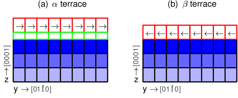
To compare the scattering from surfaces terminated at $\alpha$ and $\beta$ terraces, we terminate the substrate at a $\beta$ terrace, and incorporate an extra half unit cell of substrate atoms (in their bulk positions) into the bottom of the reconstructed overlayer for the $\alpha$ terrace case. We also reverse the relaxation amounts in the $y$ direction for the $\alpha$ terraces, relative to those for the $\beta$ terraces. Figure 4 illustrates these arrangements. Appendix B gives tables of atomic coordinates $\mathbf{r}_{jkn}$ used for the $\alpha$ and $\beta$ structure factors.

Figure 5: Calculated reflectivity of (a) (000L), (b) $(01\overline{1}L)$, and (c) $(10\overline{1}L)$ CTRs for exactly oriented surface with $\alpha$ or $\beta$ terrace terminations, with the 3H(T1) reconstruction, $\sigma_{R}=1$ Å, $\sigma_{k}=0.11$ Å.

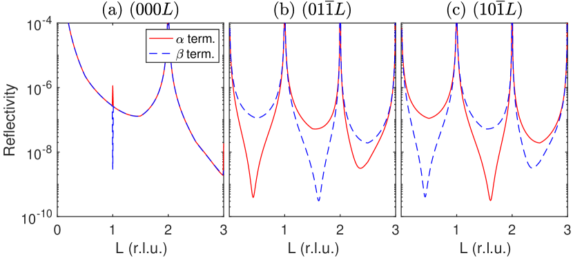
Figure 5 shows the calculated reflectivity as a function of $L$ for different integer $H_{0}K_{0}I_{0}$ values, for both $\alpha$ and $\beta$ terminations. Fits to X-ray measurements described below indicate that the GaN surface under OMVPE conditions has a 3H(T1) reconstruction, in which 3 of every 4 Ga atoms in top-layer sites shown in Fig. 2 is bonded to an adsorbed hydrogen. We thus show calculations for a surface with the 3H(T1) reconstruction, for equal fractions $\theta_{j}=1/6$ of all six domains. We use atomic form factors for each type of atom Waasmaier and Kirfel (1995) with resonant corrections for the 25.75 keV photon energy used in the experiments Henke et al. (1993), and an estimated Debye-Waller length of $\sigma_{k}=0.11$ Å  for all atoms. The (000L) CTR is insensitive to the difference between the $\alpha$ and $\beta$ terminations; both give the same intensity distribution. In contrast, the $(01\overline{1}L)$ and $(10\overline{1}L)$ CTRs show very different intensity distributions for $\alpha$ and $\beta$ terminations. There are alternating deep and shallow minima between the Bragg peaks, with the alternation being opposite for the two terminations. Furthermore, the $(01\overline{1}L)$ scattering from the $\alpha$ terrace is identical to the $(10\overline{1}L)$ scattering from the $\beta$ terrace, and vice versa, as required by symmetry. We have performed calculations using atomic coordinates for all of the GaN (0001) reconstructions found previously Walkosz et al. (2012), as well as an unreconstructed surface. All show the same qualitative behavior, with small quantitative differences. Furthermore, because the X-ray scattering is dominated by the Ga atoms, which occupy an HCP lattice, the same qualitative behavior is also obtained for an elemental HCP crystal.

II.2 Vicinal surface with reconstruction

Figure 6: Substrate unit cells (black), extra half unit cells (green) producing shift between $\alpha$ and $\beta$ terminations of neighboring terraces, and reconstructed unit cells (red), for a vicinal surface with $m=6$, $m_{\alpha}=2$, and $f_{\alpha}=1/3$. Blue shade indicates index $\ell$ of sum in Eq. (9), with final term $\ell=0$ darkest.

We now consider a vicinal surface, with a periodic array of steps. We specialize to steps normal to the $[01\overline{1}0]$ $y$ axis. We assume that the surface height decreases by a full unit cell $c$ every $m$ unit cells in $y$, so that the period of the step array is $mb$. The surface offcut angle $\gamma$ relative to (0001) is given by $\tan{\gamma}=c/(mb)$, and the surface is parallel to $(01\overline{1}2m)$ planes. The CTRs from this surface are tilted in the $Q_{y}$ direction at an angle $\gamma$ from (0001). Because of the tilt, there are $2m$ times as many CTRs as in the exactly oriented case, indexed not just by $H_{0}K_{0}I_{0}$ but also by values of $L_{0}$ from $0$ to $2m-1$. The $Q_{y}$ value varies with $L$ along the CTR according to $Q_{y}=(2\pi/b)[H_{0}+2K_{0}+(L-L_{0})/m]$, where $H_{0}K_{0}I_{0}L_{0}$ is the primary Bragg peak associated with the CTR. The spacing in $L$ along a given CTR between Bragg peak positions is $2m$, rather than unity as in the exactly oriented surface. Figure 6 shows the substrate and reconstructed unit cells used to calculate the CTRs for the vicinal surface. The width of the $\alpha$ terraces is $m_{\alpha}$ unit cells, and the width of the $\beta$ terraces is $m-m_{\alpha}$ unit cells. The $\alpha$ terrace fraction is given by $f_{\alpha}=m_{\alpha}/m$.

The reflectivity amplitude from the truncated crystal substrate is

$$r_{s}=\frac{r_{f}F_{s}}{m}\sum_{\ell=-\infty}^{0}Y^{\ell}=\frac{r_{f}F_{s}}{m}\frac{Y}{Y-1},$$ (9)

where the quantity $Y$ is now the ratio of the contribution from one unit cell to that from the unit cell at $\Delta y=-b$ beside it,

$$Y\equiv\exp(iQ_{y}b+\epsilon\,b\sin\gamma/Q_{\perp}),$$ (10)

where $Q_{\perp}=Q_{z}/\cos{\gamma}+Q_{y}\sin{\gamma}$ is the component of $\mathbf{Q}$ perpendicular to the surface. For a vicinal crystal, the scattering is built up by summing the contributions from each unit cell in the $y$ direction from $\ell=-\infty$ to $\ell=0$.

The reflectivity from the reconstructed layers on the $\alpha$ terraces can be written as

$$r_{\alpha}=\frac{r_{f}F_{\alpha}}{m}\sum_{\ell=1}^{m_{\alpha}}Y^{\ell}=\frac{r_{f}F_{\alpha}}{m}\frac{Y(Y^{m_{\alpha}}-1)}{Y-1},$$ (11)

where the unit cell structure factor $F_{\alpha}$ is given by

$$F_{\alpha}=\sum_{j}\theta_{\alpha j}\sum_{k}f_{k}\exp(-\sigma_{k}^{2}Q^{2})\sum_{n}\exp(i\mathbf{Q}\cdot\mathbf{r}_{jkn}^{\alpha}).$$ (12)

Here $\theta_{\alpha j}$ and $\mathbf{r}_{jkn}^{\alpha}$ are the domain fractions and atomic positions for the $\alpha$ terrace.

Similar expressions apply to the reflectivity from the reconstructed layers on the $\beta$ terraces,

$$r_{\beta}=\frac{r_{f}F_{\beta}}{m}\sum_{\ell=m_{\alpha}+1}^{m}Y^{\ell}=\frac{r_{f}F_{\beta}}{m}\frac{Y(Y^{m}-Y^{m_{\alpha}})}{Y-1},$$ (13)

$$F_{\beta}=\sum_{j}\theta_{\beta j}\sum_{k}f_{k}\exp(-\sigma_{k}^{2}Q^{2})\sum_{n}\exp(i\mathbf{Q}\cdot\mathbf{r}_{jkn}^{\beta}).$$ (14)

The total reflectivity amplitude is the sum of the complex amplitudes from the substrate and the reconstructed layers on the $\alpha$ and $\beta$ terraces,

$$r_{t}=r_{s}+r_{\alpha}+r_{\beta}.$$ (15)

The same expressions Eq. (7,8) given above relate the intensity reflectivity $R$ to $r_{t}$.

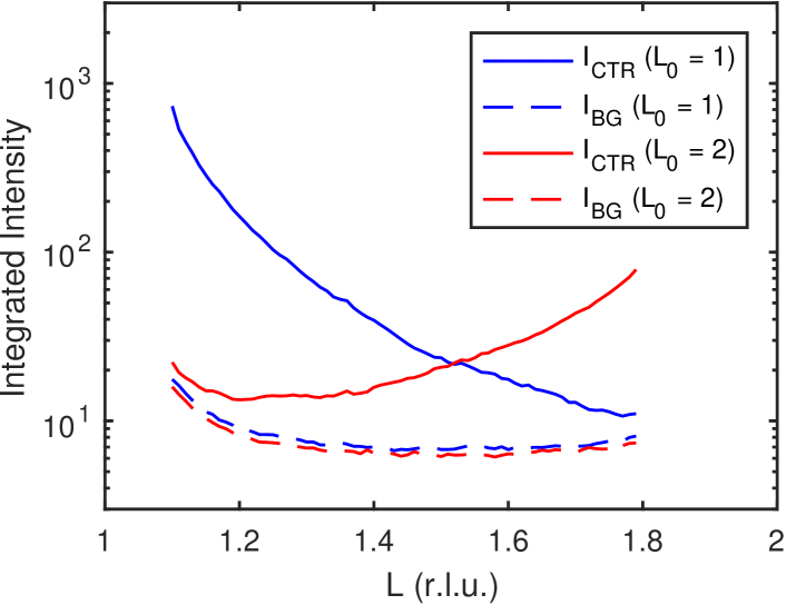
Figure 7 shows the calculated reflectivity of the $(000L_{0})$, $(01\overline{1}L_{0})$, and $(10\overline{1}L_{0})$ CTRs for $L_{0}=-1$ to $4$ for a miscut surface with three $f_{\alpha}$ values, 0.0, 0.5, and 1.0. These calculations were done for a step period of $m=100$, a surface with the 3H(T1) reconstruction with equal fractions $\theta_{\alpha j}=\theta_{\beta j}=1/6$ of all domains on both terraces, a roughness of $\sigma_{R}=1$ Å, and a Debye-Waller length of $\sigma_{k}=0.11$ Å  for all atoms. The result is insensitive to 10% changes in $m$. While as in the case of an exactly oriented surface, the $(000L_{0})$ CTRs are identical for $f_{\alpha}=0$ and $f_{\alpha}=1$, they are very different for $f_{\alpha}=0.5$, with the CTRs for even $L_{0}$ becoming stronger and the CTRs for odd $L_{0}$ becoming very weak. The $(01\overline{1}L_{0})$ and $(10\overline{1}L_{0})$ CTRs have a more monotonic dependence on $f_{\alpha}$. For $f_{\alpha}=0$ and $f_{\alpha}=1$, there are alternating stronger and weaker intensities between the Bragg peaks, with the alternation being opposite for $(01\overline{1}L_{0})$ and $(10\overline{1}L_{0})$. For $f_{\alpha}=0.5$, the intensities between the Bragg peaks are about the same, and there is no difference between the $(01\overline{1}L_{0})$ and $(10\overline{1}L_{0})$ CTRs. The $(01\overline{1}L_{0})$ CTRs with $f_{\alpha}=X$ are identical to the $(10\overline{1}L_{0})$ CTRs with $f_{\alpha}=1-X$, for any value $X$. As with the exactly oriented surface, other reconstructions or HCP bulk structures show the same qualitative behavior.

Figure 7: Calculated reflectivities of CTRs for an $m=100$ vicinal surface with the 3H(T1) reconstruction, $\sigma_{R}=1$ Å, and $\sigma_{k}=0.11$ Å. Top row: (0 0 0 L); middle row: $(01\overline{1}L)$; bottom row: $(10\overline{1}L)$. Black, red, green, blue, cyan, and magenta curves are for $L_{0}=-1$ to $4$, respectively. Values of $f_{\alpha}$ for each column are given at the top.

Figure 8: Calculated reflectivity of selected CTRs as a function of terrace fraction $f_{\alpha}$, for fixed values of $L$ near $L=1.6$. These curves use a fixed $\sigma_{R}=0.9$ Å  and $\sigma_{k}=0.11$ Å.

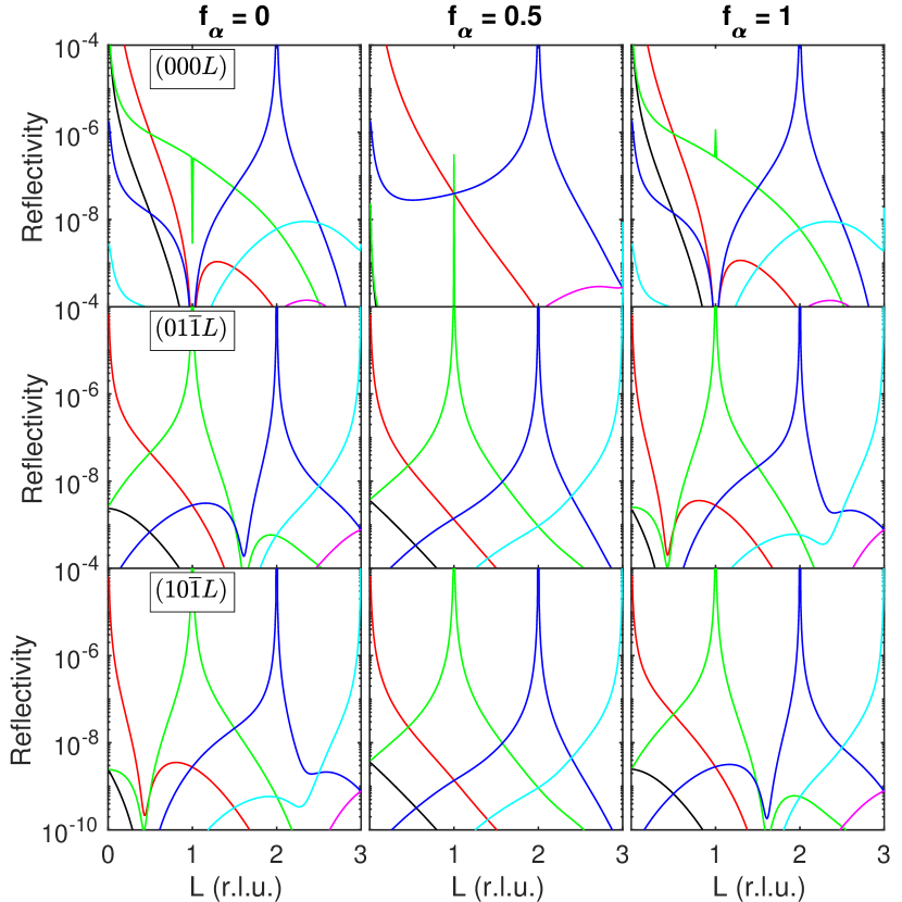
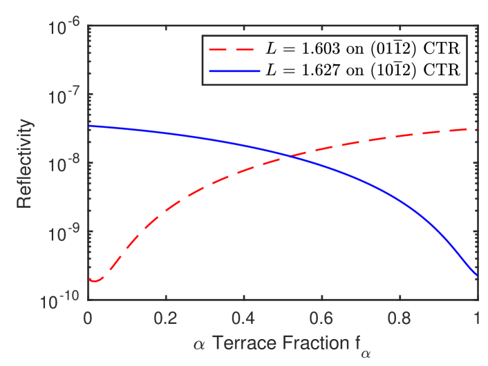
Figure 8 shows calculations of the reflectivity as a function of $f_{\alpha}$ at positions near $L=1.6$ on the $(01\overline{1}2)$ and $(10\overline{1}2)$ CTRs, for a surface with the 3H(T1) reconstruction. Here we use a roughness of $\sigma_{R}=0.9$ Å  to match the experimental fits described below. The variation in reflectivity is almost monotonic in $f_{\alpha}$ at these positions. These curves are used below to extract $f_{\alpha}(t)$ during dynamic transitions.

Table 1: For each of four OMVPE conditions, we list the net growth rate $G$ in ML/s, where 1 ML $=c/2=2.6$ Å, as well as values of $f_{\alpha}^{ss}$, $\sigma_{R}$, and $\chi^{2}$ from fits to reflectivity for each of 5 reconstructions.

Growth	TEGa flow	H2 frac.	Net growth		3H(T1)	Ga(T4)	NH(H3)+	NH(H3)+	NH(H3)
condition	($\mu$mole	in	rate				H(T1)	NH2(T1)
index	/min)	carrier	(ML/s)
				$f_{\alpha}^{ss}$	0.111	0.144	0.098	0.106	0.095
1	0.000	50%	-0.0018	$\sigma_{R}$(Å)	0.91	1.53	1.14	1.07	1.10
				$\chi^{2}$	106	130	187	200	167
				$f_{\alpha}^{ss}$	0.461	0.476	0.460	0.460	0.459
2	0.000	0%	0.0000	$\sigma_{R}$(Å)	1.13	1.53	1.39	1.34	1.37
				$\chi^{2}$	57	81	76	67	99
				$f_{\alpha}^{ss}$	0.811	0.670	0.876	0.869	0.869
3	0.033	50%	0.0109	$\sigma_{R}$(Å)	1.03	1.77	1.44	1.40	1.40
				$\chi^{2}$	118	218	205	248	168
				$f_{\alpha}^{ss}$	0.868	0.942	0.892	0.879	0.891
4	0.033	0%	0.0127	$\sigma_{R}$(Å)	0.57	1.28	1.09	1.03	1.05
				$\chi^{2}$	80	112	174	220	135

III Surface X-ray Scattering Measurements and Fits

To characterize the behavior of $A$ and $B$ steps in GaN (0001) surfaces, we performed in situ measurements of the CTRs during growth and evaporation in the OMVPE environment. We used a chamber and goniometer at the Advanced Photon Source beamline 12ID-D, which was designed for in situ surface X-ray scattering studies during growth Ju et al. (2017). A micron-scale X-ray beam illuminated a small surface area having a uniform step azimuth. To obtain sufficient signal, we used a wide-bandwidth “pink” beam setup similar to that described previously Ju et al. (2018, 2019). The beam incident on the sample had a typical intensity of $1.4\times 10^{12}$ photons per second at $E=25.75$ keV, in a spot size of $10\times 10$ $\mu$m. At the $2^{\circ}$ incidence angle, this illuminated an area of $10\times 300$ $\mu$m. X-ray scattering patterns were recorded using a photon counting area detector with a GaAs sensor having 512 $\times$ 512 pixels, 55 $\mu$m pixel size, located $1.1$ m from the sample (Amsterdam Scientific Instruments LynX 1800).

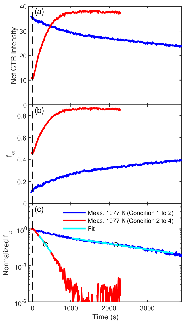
Two types of measurements were performed. We determined the steady-state terrace fractions $f_{\alpha}^{ss}$ under four different growth/evaporation conditions by scanning the detector along the $(01\overline{1}L)$ and $(10\overline{1}L)$ CTRs while continuously maintaining steady-state growth or evaporation. We also observed the dynamics of the change in $f_{\alpha}$ by recording the intensity at a fixed detector position near $L=1.6$ as a function of time before and after an abrupt change between conditions.

We studied four OMVPE conditions, summarized in Table 1. Under the conditions studied, deposition is transport limited, with the deposition rate proportional to the supply of the Ga precursor (triethylgallium, TEGa), with a large excess of the N precursor (NH₃) constantly supplied. We investigated conditions of zero deposition (no supply of TEGa) as well as deposition at a TEGa supply of 0.033 $\mu$mole/min. The NH₃ flow in both cases was 2.7 slpm or 0.12 mole/min, and the total pressure was 267 mbar. The V/III ratio during deposition was thus $3.6\times 10^{6}$. For both of these conditions, we studied two carrier gas compositions: 50% H₂ + 50% N₂, and 0% H₂ + 100% N₂. The addition of H₂ to the carrier gas enhances evaporation of GaN, so that the net growth rate (deposition rate minus evaporation rate) is slightly lower; at zero deposition rate, the net growth rate is negative. We determined the net growth rate for all four conditions as described in Appendix C. These values are given in Table 1. Substrate temperatures were calibrated to within $\pm 5$ K using laser interferometry from a standard sapphire substrate Ju et al. (2017). While we used the same heater temperature for all conditions, the calibration indicates that the substrate temperature was slightly higher in 50% H₂ (1080 K) than in 0% H₂ (1073 K).

Figure 9: AFM image of steps of height c/2 (2.6 Å) on the GaN substrate used in X-ray measurements. To emphasize the positions of steps, we plot the amplitude error signal, which is proportional to the height gradient in the scan direction $(y)$. Image was obtained ex situ at room $T$ after an anneal for 300s at 1118 K in zero-growth conditions (0% H₂, 0 TEGa). Average fraction over a $2\times 2$ $\mu$m area of “even” terraces (marked black at side) is 0.47. The average double-step spacing of $w=57.3$ nm corresponds to an offcut of $\tan^{-1}(c/w)=0.52^{\circ}$.

Figure 10: Profile of split CTRs showing offcut. Peaks correspond to the (0002), (0001), and (0000) CTRs at $L=0.9$. Measured at $T=1170$ K during growth at $0.053$ $\mu$mole/min TEGa, 50% H₂. The splitting of the CTRs $\Delta Q_{y}=0.0110$ Å^-1 corresponds to an offcut of $\tan^{-1}[\Delta Q_{y}/(2\pi/c)]=0.52^{\circ}$.

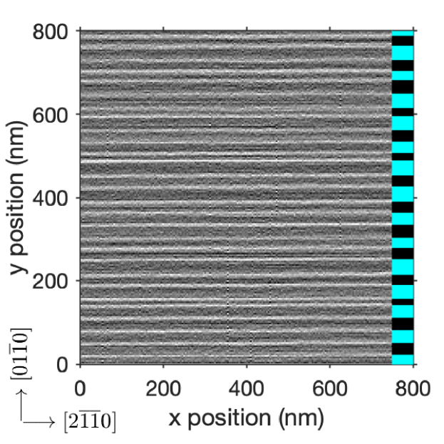
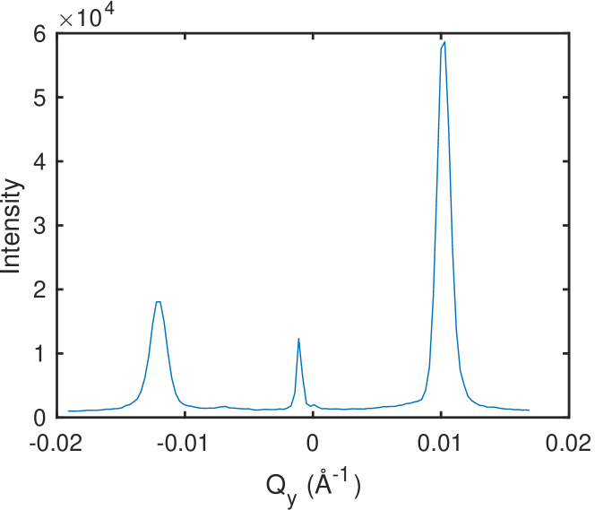
The substrate used was a GaN single crystal . Figure 9 shows its initial surface morphology determined by ex situ atomic force microscopy (AFM) following an anneal at 1118 K for 300 s in zero-growth conditions (0% H₂, 0 TEGa). One can see straight steps almost perpendicular to $y$ over large areas. An analysis of the step spacing shows a slight tendency towards pairing, with one of the two alternating terrace types having an area fraction of 0.47. AFM is insensitive to whether this fraction corresponds to the $\alpha$ or $\beta$ terraces. We also characterized the offcut by measuring the splitting of the CTRs. Figure 10 shows a transverse cut through the CTRs in the $Q_{y}$ direction near (000L) at $L=0.9$. Both the AFM and X-ray measurements give a double-step spacing of $w=573$ Å  corresponding to an offcut of $0.52^{\circ}$. To relate the $\alpha$ terrace fraction to the behavior of $A$ and $B$ steps, it is critical to determine the sign of the step azimuth. By making measurements as a function of $Q_{z}$, we verified that the peak at high $Q_{y}$ is the CTR coming from (0000), while the peak at low $Q_{y}$ is the (0002) CTR. This confirms that the “downstairs” direction of the vicinal surface is in the $+y$ or $[01\overline{1}0]$ direction, as drawn in Fig. 2. It is also useful to know the precise angle of the step azimuth with respect to the crystal planes, which determines the kink density and thus some kinetic coefficients. X-ray measurements found this to be $5^{\circ}$ off of the $[01\overline{1}0]$ direction towards $[10\overline{1}0]$. With this low-dislocation-density substrate and the low growth rates used, we did not observe the previously reported instability to step bunching during growth Murty et al. (2000).

Figure 11: Detector image from $(01\overline{1}L)$ scan at for condition 4 ($0.033\mu$mol/min TEGa, 0% H₂), showing intensity maxima from Ewald sphere cutting through CTRs from the $(01\overline{1}1)$ and $(01\overline{1}2)$ Bragg peaks. Position of central pixel, marked by cross, is $(01\overline{1}L)$ with $L=1.55$. Dark area on right is shadow of slits, white vertical line is gap in pixels between detector chips. White pixels are ignored due to excessive detector noise.

Figure 12: Cut through reciprocal space at $L=Q_{z}c/2\pi=1.55$, showing $(01\overline{1}1)$ and $(01\overline{1}2)$ CTRs. The in-plane $Q_{x}$ and $Q_{y}$ coordinates have been expressed as in-plane radial and transverse components $\Delta Q_{rad}$ and $\Delta Q_{trans}$ relative to the central pixel at position $(01\overline{1}L)$. Rectangles give regions integrated to give CTR intensities and associated backgrounds.

Figure 13: Integrated total CTR and background intensities for the $(01\overline{1}1)$ and $(01\overline{1}2)$ CTRs, as a function of $L$ between $1.1$ and $1.8$, for condition 4 ($0.033$  $\mu$mol/min TEGa, 0% H₂).

Figure 14: Symbols show measured net intensities of the $(01\overline{1}L_{0})$ CTRs (top row) and the $(10\overline{1}L_{0})$ CTRs (bottom row) for $L_{0}=0,1,2,3$ at each of four conditions. Curves show fits of all CTRs using the 3H(T1) reconstruction to obtain steady-state $\alpha$ terrace fraction $f_{\alpha}^{ss}$ at each condition.

Figure 15: Surface reconstruction phase diagram for GaN (0001), calculated in Walkosz et al. (2012). Green rectangle shows estimated position of our experimental conditions, calculated in Appendix A. Five shaded reconstructions near these conditions were considered in fits shown in Table 1.

III.1 CTR measurements

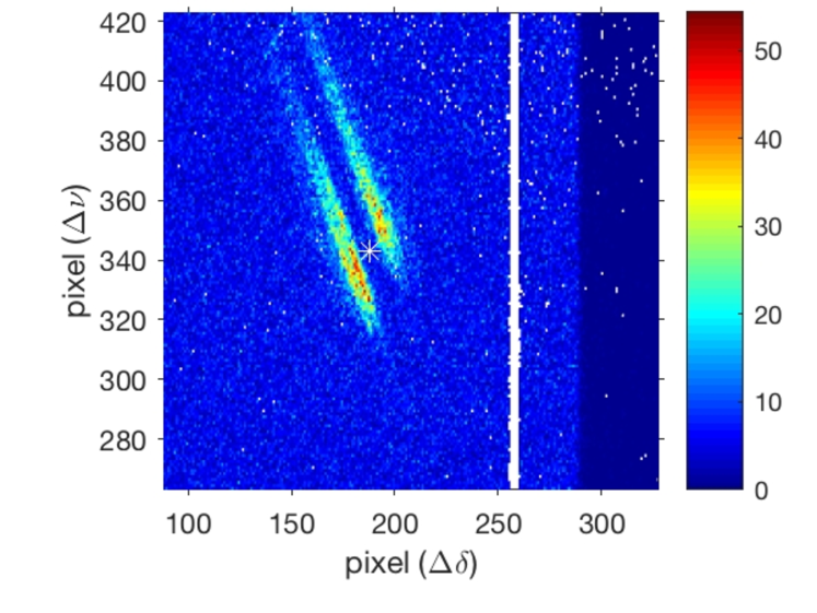
To process the X-ray data from the area detector, raw images were first corrected for detector flatfield, eliminating pixels with excessive noise, and the signal was normalized to the incident intensity. Figure 11 shows a typical corrected detector image, with streaks from the $(01\overline{1}1)$ and $(01\overline{1}2)$ CTRs. Because of the $\sim 1\%$ energy bandwidth of the pink beam Ju et al. (2019), the CTRs are broadened radially as well as being extended in the $Q_{z}$ direction. To convert the images along an $L$ scan to reciprocal space, the $Q_{x}Q_{y}Q_{z}$ coordinates of each pixel in each image were first calculated. The out-of-plane coordinate $Q_{z}$ or $L$ varies across each image, following the Ewald sphere. The in-plane coordinates $Q_{x}$ and $Q_{y}$ were converted to in-plane radial and transverse components $\Delta Q_{rad}$ and $\Delta Q_{trans}$ relative to the central position. The intensities and $L$ values of each image were interpolated onto a fixed grid of $\Delta Q_{rad}$ and $\Delta Q_{trans}$. We then interpolate the sequence of intensities from the scan at each $\Delta Q_{rad}$ and $\Delta Q_{trans}$ onto a grid of fixed $L$ values.

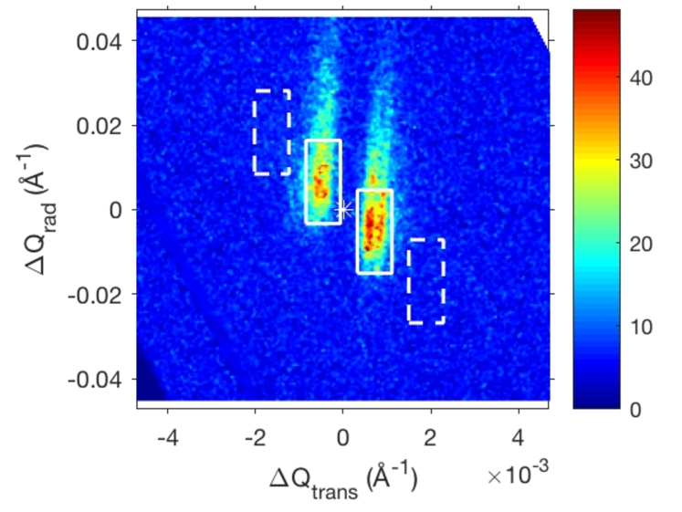
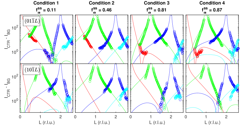
Figure 12 shows a typical cut through reciprocal space at fixed $L$. The peaks from the $(01\overline{1}1)$ and $(01\overline{1}2)$ CTRs are conveniently separated in $\Delta Q_{trans}$ because of the $5^{\circ}$ deviation of the step azimuth from $[01\overline{1}0]$; if the deviation was zero, the peaks would overlap at $\Delta Q_{trans}=0$ because of the broadening in $\Delta Q_{rad}$. Regions of $\Delta Q_{trans}$ and $\Delta Q_{rad}$ surrounding each CTR were defined to integrate the total intensity, with positions that vary with $L$ to follow the CTRs. Likewise adjacent regions were defined to integrate an equivalent volume of background scattering. Such regions are shown as rectangles in Fig. 12. Figure 13 shows the mean total CTR intensities and backgrounds in these regions as a function of $L$ for the scan between $L=1.1$ and $L=1.8$ for condition 4. The net CTR intensity was calculated by subtracting the background from the total for that CTR. We ran scans from $L=0.4$ to $L=0.9$, $L=1.1$ to $L=1.8$, and $L=2.15$ to $L=2.6$ on the $(01\overline{1}L)$ and $(10\overline{1}L)$ CTRs, skipping over the Bragg peaks to avoiding having the high intensity strike the detector. The $L$ range covered on each CTR varied depending upon the region covered by the detector in reciprocal space during the scan. Figure 14 shows the measured net CTR intensities as a function of $L$, for both the $(01\overline{1}L)$ and $(10\overline{1}L)$ CTRs and at all four conditions. Only data points at which the total and background regions were fully captured on the detector without shadowing from the chamber window were kept. This eliminated all of the data points for the $(10\overline{1}0)$ CTR. The qualitative behavior agrees with that expected from a variation in $f_{\alpha}$ shown in Fig. 7, with alternating higher and lower intensities between the Bragg peaks in some cases, and opposite behavior of the two CTRs.

In order to determine whether exposure to the X-ray beam was affecting the OMVPE growth process, we periodically scanned the sample position while monitoring the CTR intensity. For the conditions reported here, there was no indication that the spot which had been illuminated differed in any way from the neighboring regions. During growth at higher temperatures (e.g. $1250$ K), we did observe local effects of the X-ray beam on the surface morphology.

III.2 Fits to steady-state CTRs

To obtain values of the steady-state terrace fraction $f_{\alpha}^{ss}$ for each of the four conditions, we fit the measured CTR intensities as a function of $L$ using the expressions developed in Section II above. For each condition, the measurements of both the $(01\overline{1}L)$ and $(10\overline{1}L)$ CTRs were simultaneously fit. In addition to a single value of $f_{\alpha}$, parameters varied in the fit included a surface roughness $\sigma_{R}$ and intensity scale factors for each CTR. In the calculations we use $m=100$, which produces negligible difference in $R$ compared with using the experimental value of $w/b=103.4$. Note that we allow $f_{\alpha}=m_{\alpha}/m$ to vary continuously, even though Eqs. (11) and (13) were developed for integer $m_{\alpha}$. We used equal fractions $\theta_{\alpha j}=\theta_{\beta j}=1/6$ of all domains on both terraces, and fit to $\log(I)$ with equal weighting of all points. Since no fractional-order diffraction peaks from long-range ordered reconstructions are observed, we expect that the domain structure has a short correlation length and all domains are present.

Figure 16: Circles show experimental values of steady-state $\alpha$ terrace fraction as a function of growth rate obtained from fits to $(01\overline{1}L)$ and $(10\overline{1}L)$ CTRs using the 3H(T1) reconstruction, showing monotonic increase of $f_{\alpha}^{ss}$ with increasing $G$. Also shown are BCF model calculations described below.

Figure 17: Dynamics upon changing conditions. Blue curves: Evolution after changing from condition 1 to condition 2 at $t=0$, determined from the $(10\overline{1}2)$ CTR at $L=1.627$. Red curves: Evolution after changing from condition 2 to condition 4 at $t=0$, determined from the $(01\overline{1}2)$ CTR at $L=1.603$. (a) Measured net CTR intensities. (b) Evolution of terrace fraction $f_{\alpha}$ calculated from CTR intensities. (c) Normalized $f_{\alpha}$ change, plotted on a log scale, with a region fitted to a straight line to get the relaxation times $2177$ s and $341$ s as shown by circles.

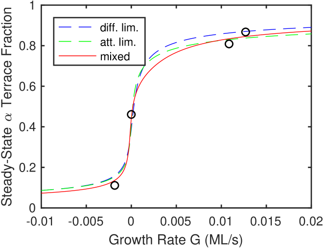
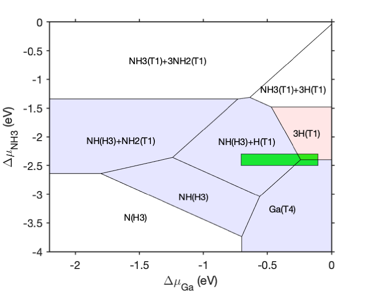
We performed fits using different potential surface reconstructions. Figure 15 shows the calculated reconstruction phase diagram for the GaN (0001) surface in the OMVPE environment Walkosz et al. (2012), as a function of Ga and NH₃ chemical potentials. Based on the chemical potential values that correspond to our experimental conditions estimated in Appendix A, shown by the green rectangle, we considered the five reconstructions highlighted in Fig. 15. (The estimate for $\Delta\mu_{Ga}$ has a large uncertainty because it depends on the nitrogen potential produced by decomposition of NH₃.) Table 1 shows the values of $f_{\alpha}^{ss}$, $\sigma_{R}$, and the goodness-of-fit parameter $\chi^{2}$ from fits to reflectivity at four conditions for each of five reconstructions. The qualitative results for the variation of $f_{\alpha}^{ss}$ with growth condition are independent of which reconstruction is assumed: $f_{\alpha}^{ss}$ increases monotonically as the net growth rate $G$ increases. The 3H(T1) reconstruction gives the best fit (minimum $\chi^{2}$) of the five potential reconstructions, for all four conditions. This is consistent with recent results on GaN (0001) reconstructions in the OMVPE environment, which found an even larger phase field for the 3H(T1) structure Kempisty and Kangawa (2019). Fig. 14 compares the fits with the 3H(T1) reconstruction to the measured CTR intensities. Figure 16 shows a plot of the resulting $f_{\alpha}^{ss}$ vs. net growth rate. As we shall see below, the increase of $f_{\alpha}^{ss}$ with increasing growth rate indicates the nature of difference between the kinetics of adatom attachment at $A$ and $B$ steps: for GaN in the OMVPE environment, $A$ steps have faster kinetics.

III.3 Dynamics of $f_{\alpha}$

We also observed the dynamics of the change in $f_{\alpha}$ by recording the intensity at a fixed detector position as a function of time before and after an abrupt change between conditions, as shown in Figure 17(a). We chose positions near $L=1.6$ where the reflectivity changes almost monotonically with $f_{\alpha}$, as shown in Fig. 8. It is thus straightforward to convert these intensity evolutions to variations in $f_{\alpha}$ by normalizing them to match the predicted change in reflectivity for the transition in $f_{\alpha}^{ss}$, and then inverting the $R(f_{\alpha})$ relation to obtain $f_{\alpha}(t)$. We assume the surface roughness is not a function of condition, and use the average value of $\sigma_{R}=0.9$ Å  from the 3H(T1) fits to calculate $R(f_{\alpha})$. The resulting $f_{\alpha}(t)$ are shown in Fig. 17(b). To extract characteristic relaxation times for these transitions, we plot the normalized change in $f_{\alpha}$, i.e. $[f_{\alpha}-f_{\alpha}(t=\infty)]/[f_{\alpha}(t=0)-f_{\alpha}(t=\infty)]$, on a log scale in Fig. 17(c). We fit the region indicated with a line and interpolated to obtain the $1/e$ decay point of these curves.

IV Burton-Cabrera-Frank theory for vicinal c-plane surfaces

To understand the behavior of the terrace fraction at steady-state and as a function of time after a change in growth rate, we have developed a model based on BCF theory for vicinal surfaces with a sequence of steps Jeong and Williams (1999). This type of one-dimensional model considers adatom diffusion on terraces with boundary conditions at the steps defining the terrace edges, and has been used extensively to understand the step-bunching instability Guin et al. (2020); Li et al. (2016); Bellmann et al. (2017); Dufay et al. (2007); Pierre-Louis (2003a); Pimpinelli and Videcoq (2000), step pairing Pierre-Louis and Métois (2004), step width fluctuations Patrone et al. (2010), growth mode transitions Ranguelov et al. (2007), and competitive adsorption Hanada (2019). Typically, all steps in a sequence are assumed have identical properties. In our case, we consider an alternating sequence of two types of terraces, $\alpha$ and $\beta$, and two types of steps, $A$ and $B$, with properties that can differ, as shown in Figs. 2 and 18. Similar BCF models of alternating $A$ and $B$ steps have been considered previously Załuska-Kotur et al. (2011, 2010); Xie et al. (2006). Here we include the effects of step transparency (also known as step permeability, the transmission of adatoms across steps) Pierre-Louis (2003b, a); Ranguelov et al. (2007) and step-step repulsion Jeong and Williams (1999); Patrone et al. (2010).

In this section we develop a quasi-steady-state expression for the dynamics of the terrace fraction $f_{\alpha}$, and give an exact solution using matrices. Examples of the adatom distributions and $f_{\alpha}$ dynamics are shown. Using further generally applicable assumptions, we develop a simplified analytical solution, and then consider cases of diffusion- or attachment-limited kinetics, and non-transparent or highly transparent steps.

IV.1 Exact quasi-steady-state solution

The continuity equation for the rate of change in the adatom density per unit area $\rho_{i}$ on terrace type $i=\alpha$ or $\beta$ is written as

$$\frac{\partial\rho_{i}}{\partial t}=D\nabla^{2}\rho_{i}-\frac{\rho_{i}}{\tau}+F,$$ (16)

where $D$ is the adatom diffusivity, $\tau$ is the adatom lifetime before evaporation, and $F$ is the deposition flux of adatoms per unit time and area. The four boundary conditions for the flux at the steps terminating each type of terrace can be written as

$$J_{\alpha}^{+} =-D\nabla\rho_{\alpha}^{+}=+\kappa_{-}^{A}(\rho_{\alpha}^{+}-\rho_{eq}^{A})+\kappa_{0}^{A}(\rho_{\alpha}^{+}-\rho_{\beta}^{-}),$$ (17)

$$J_{\alpha}^{-} =-D\nabla\rho_{\alpha}^{-}=-\kappa_{+}^{B}(\rho_{\alpha}^{-}-\rho_{eq}^{B})-\kappa_{0}^{B}(\rho_{\alpha}^{-}-\rho_{\beta}^{+}),$$ (18)

$$J_{\beta}^{+} =-D\nabla\rho_{\beta}^{+}=+\kappa_{-}^{B}(\rho_{\beta}^{+}-\rho_{eq}^{B})+\kappa_{0}^{B}(\rho_{\beta}^{+}-\rho_{\alpha}^{-}),$$ (19)

$$J_{\beta}^{-} =-D\nabla\rho_{\beta}^{-}=-\kappa_{+}^{A}(\rho_{\beta}^{-}-\rho_{eq}^{A})-\kappa_{0}^{A}(\rho_{\beta}^{-}-\rho_{\alpha}^{+}),$$ (20)

where $J_{i}$ is the adatom flux on terrace $i$, $\kappa_{+}^{j}$ and $\kappa_{-}^{j}$ are the kinetic coefficients for adatom attachment at a step of type $j=A$ or $B$ from below or above, respectively, $\kappa_{0}^{j}$ is the kinetic coefficient for transmission across the step, $\rho_{eq}^{j}$ is the equilibrium adatom density at a step of type $j$, and the $+$ or $-$ superscripts on $J_{i}$, $\rho_{i}$, and $\nabla\rho_{i}$ indicate evaluation at the terrace boundaries $y=+w_{i}/2$ or $y=-w_{i}/2$, respectively, where $w_{i}$ is the width of the terraces of type $i$ and the spatial coordinate $y$ is taken to be zero in the center of each terrace. As shown in Fig. 18, the negative “upstairs” boundary of a terrace of type $i=\alpha$ $(\beta)$ at $y=-w_{i}/2$ is a step of type $j=B$ $(A)$, while the positive “downstairs” boundary at $y=+w_{i}/2$ is a step of type $j=A$ $(B)$, respectively. A standard positive ES barrier is given by $\kappa_{+}^{j}>\kappa_{-}^{j}$.

Figure 18: Schematic of alternating terraces and steps of BCF model for HCP basal plane surfaces, showing kinetic coefficients for the $A$ and $B$ steps.

The velocity $v_{j}$ of the $j$ type step can be obtained from the adatom fluxes arriving from each side, giving

$$v_{A} =\left(J_{\alpha}^{+}-J_{\beta}^{-}\right)/\rho_{0},$$ (21)

$$v_{B} =\left(J_{\beta}^{+}-J_{\alpha}^{-}\right)/\rho_{0},$$ (22)

where $\rho_{0}$ is the density of lattice sites per unit area. In the boundary conditions Eqs. (17-20) we have neglected the “advective” terms $-\rho_{i}^{\pm}v_{j}$ due to the moving boundary Guin et al. (2020), under the assumption that the adatom coverages are small, $\rho_{i}<<\rho_{0}$.

We assume that the adatom density profiles $\rho_{i}(y)$ have reached a quasi-steady-state where we can set $\partial\rho_{i}/\partial t=0$ in the continuity equation Eq. (16). We still allow the terrace widths $w_{i}$ to evolve relatively slowly with time. At quasi-steady-state, the general solution for the adatom densities satisfying Eq. (16) is

$$\rho_{i}=F\tau+C_{1i}\cosh\left(\frac{y}{\sqrt{D\tau}}\right)+C_{2i}\sinh\left(\frac{y}{\sqrt{D\tau}}\right),$$ (23)

where $C_{1i}$ and $C_{2i}$ are coefficients to be determined from the boundary conditions for each terrace type $i=\alpha$ or $\beta$. The gradient $\nabla\rho_{i}$ with respect to $y$ is then

$$\nabla\rho_{i}=\frac{C_{1i}}{\sqrt{D\tau}}\sinh\left(\frac{y}{\sqrt{D\tau}}\right)+\frac{C_{2i}}{\sqrt{D\tau}}\cosh\left(\frac{y}{\sqrt{D\tau}}\right).$$ (24)

If we define the coefficients

$$c_{i}\equiv\cosh\left(\frac{w_{i}}{2\sqrt{D\tau}}\right),$$ (25)

$$s_{i}\equiv\sinh\left(\frac{w_{i}}{2\sqrt{D\tau}}\right),$$ (26)

for terrace types $i=\alpha$ and $\beta$, and dimensionless step kinetic parameters

$$p_{j} \equiv(\tau/D)^{1/2}\,\,\kappa_{+}^{j},$$ (27)

$$q_{j} \equiv(\tau/D)^{1/2}\,\,\kappa_{-}^{j},$$ (28)

$$r_{j} \equiv(\tau/D)^{1/2}\,\,\kappa_{0}^{j},$$ (29)

for step types $j=A$ and $B$, then we can use the quasi-steady-state solution Eq. (23,24) to write the boundary conditions Eq. (17-20) as

$$\mathcal{M}\mathcal{C}=\mathcal{B},$$ (30)

where $\mathcal{M}$ is a matrix given by

$$\mathcal{M}=\begin{bmatrix}+[s_{\alpha}+(q_{A}+r_{A})c_{\alpha}]&+[c_{\alpha}+(q_{A}+r_{A})s_{\alpha}]&-r_{A}c_{\beta}&+r_{A}s_{\beta}\\ +[s_{\alpha}+(p_{B}+r_{B})c_{\alpha}]&-[c_{\alpha}+(p_{B}+r_{B})s_{\alpha}]&-r_{B}c_{\beta}&-r_{B}s_{\beta}\\ -r_{B}c_{\alpha}&+r_{B}s_{\alpha}&+[s_{\beta}+(q_{B}+r_{B})c_{\beta}]&+[c_{\beta}+(q_{B}+r_{B})s_{\beta}]\\ -r_{A}c_{\alpha}&-r_{A}s_{\alpha}&+[s_{\beta}+(p_{A}+r_{A})c_{\beta}]&-[c_{\beta}+(p_{A}+r_{A})s_{\beta}]\end{bmatrix}$$ (31)

and the vectors $\mathcal{C}$ and $\mathcal{B}$ are given by

$$\mathcal{C}=\begin{bmatrix}C_{1\alpha}\\ C_{2\alpha}\\ C_{1\beta}\\ C_{2\beta}\end{bmatrix},$$ (32)

$$\mathcal{B}=\begin{bmatrix}q_{A}(\rho_{eq}^{A}-F\tau)\\ p_{B}(\rho_{eq}^{B}-F\tau)\\ q_{B}(\rho_{eq}^{B}-F\tau)\\ p_{A}(\rho_{eq}^{A}-F\tau)\end{bmatrix}.$$ (33)

The solution for the values of the four coefficients $C_{1i}$ and $C_{2i}$ of Eq. (23) is given by

$$\mathcal{C}=\mathcal{M}^{-1}\mathcal{B},$$ (34)

where $\mathcal{M}^{-1}$ is the inverse of $\mathcal{M}$.

The quasi-steady-state step velocities can then be evaluated from expressions obtained using Eqs. (17-24),

$$v_{A} =-\sqrt{\frac{D}{\tau}}\left(\frac{s_{\alpha}C_{1\alpha}+c_{\alpha}C_{2\alpha}+s_{\beta}C_{1\beta}-c_{\beta}C_{2\beta}}{\rho_{0}}\right),$$ (35)

$$v_{B} =-\sqrt{\frac{D}{\tau}}\left(\frac{s_{\alpha}C_{1\alpha}-c_{\alpha}C_{2\alpha}+s_{\beta}C_{1\beta}+c_{\beta}C_{2\beta}}{\rho_{0}}\right).$$ (36)

The final relationships needed are those between the equilibrium adatom densities at the steps $\rho_{eq}^{j}$ and the terrace widths. These relationships reflect an effective repulsion between the steps owing to entropic and strain effects Jeong and Williams (1999); Patrone et al. (2010). In our case, with two different types of steps, we use the relations

$$\rho_{eq}^{j}=\rho_{eq}^{0}\exp(\mu_{j}/kT),$$ (37)

where $\rho_{eq}^{0}$ is the equilibrium adatom density at zero growth rate, and the chemical potentials $\mu_{j}$ for the $j=A$ and $B$ steps are

$$\frac{\mu_{A}}{kT}=-\frac{\mu_{B}}{kT}=\mathbf{M}=\left(\frac{\ell_{\beta}}{w_{\beta}}\right)^{3}-\left(\frac{\ell_{\alpha}}{w_{\alpha}}\right)^{3}.$$ (38)

Here the $\ell_{i}$ are two step repulsion lengths, that can differ for the two types of terraces.

We consider the overall vicinal angle of the surface to fix the sum $w$ of the widths of $\alpha$ and $\beta$ terraces, so that the widths can be expressed as $w_{i}=f_{i}w$, where there is one independent terrace fraction $f_{\alpha}$, and the other is given by $f_{\beta}=1-f_{\alpha}$. In this case we can express the step chemical potentials as

$$\mathbf{M}(f_{\alpha})=\left(\frac{\ell}{w}\right)^{3}\left[\left(\frac{1-f_{\alpha}^{0}}{1-f_{\alpha}}\right)^{3}-\left(\frac{f_{\alpha}^{0}}{f_{\alpha}}\right)^{3}\right],$$ (39)

where the coefficients $\ell$ and $f_{\alpha}^{0}$ are related to the $\ell_{i}$ by

$$\ell_{\alpha} =f_{\alpha}^{0}\ell,$$ (40)

$$\ell_{\beta} =(1-f_{\alpha}^{0})\ell.$$ (41)

where $f_{\alpha}^{0}$ is the terrace fraction at zero growth rate.

The net growth rate $G$ in monolayers per second is proportional to the sum of the step velocities,

$$G=\frac{v_{A}+v_{B}}{w}=-\sqrt{\frac{D}{\tau}}\left(\frac{2s_{\alpha}C_{1\alpha}+2s_{\beta}C_{1\beta}}{w\rho_{0}}\right).$$ (42)

The rate of change of the $\alpha$ terrace fraction $f_{\alpha}$ is proportional to the step velocity difference,

$$\frac{df_{\alpha}}{dt}=\frac{v_{A}-v_{B}}{w}=\sqrt{\frac{D}{\tau}}\left(\frac{2c_{\beta}C_{2\beta}-2c_{\alpha}C_{2\alpha}}{w\rho_{0}}\right).$$ (43)

This equation can be integrated to solve for the evolution of $f_{\alpha}(t)$ at quasi-steady-state. To obtain the full steady-state value of $f_{\alpha}$, the $A$ and $B$ step velocities must be equal and stable against fluctuations,

$$\frac{df_{\alpha}}{dt}=0,$$ (44)

$$\frac{\partial(df_{\alpha}/dt)}{\partial f_{\alpha}}<0.$$ (45)

When the net growth rate is zero and the terrace fraction has reached it full steady-state value, the step velocities are both zero, the diffusion fluxes are zero, the adatom densities are constant at a value $\rho_{\alpha}=\rho_{\beta}=\rho_{eq}^{A}=\rho_{eq}^{B}=\rho_{eq}^{0}$, and $\mu_{A}=-\mu_{B}=0$. One can see that the parameter $f_{\alpha}^{0}$ is the full steady-state value of $f_{\alpha}$ at zero growth rate.

Figure 19: Rate of change of the terrace fraction $df_{\alpha}/dt$ as a function of terrace fraction $f_{\alpha}$, calculated from Eq. (43) with parameter values given in Table 2. The steady-state values of $f_{\alpha}$ are marked with a circle.

Figure 20: Excess adatom density $\rho_{i}-\rho_{eq}^{0}$ on a sequence of $\alpha$ and $\beta$ terraces corresponding to the steady-state solution, calculated with parameter values given in Table 2, for $F=0$, $G=-0.00184$ ML/s.

IV.2 Calculation of steady-state and dynamics

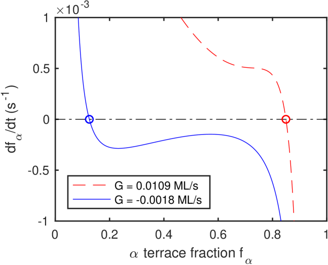
Here we show some examples calculated from the BCF theory. Figure 19 shows the quasi-steady-state rate of change of the terrace fraction $df_{\alpha}/dt$ as a function of terrace fraction $f_{\alpha}$, calculated from Eq. (43) with parameter values given in Table 2. One curve is for a situation with no deposition flux, $F=0$, where evaporation causes the net growth rate to be negative, $G=-0.00184$ ML/s, while the other is for a deposition flux of $F=1.43\times 10^{17}$ m^-2s^-1, giving a positive net growth rate of $G=0.0109$ ML/s. The steady-state values of $f_{\alpha}$ where $df_{\alpha}/dt=0$ are marked. For these parameters there is only a single steady-state solution for each curve, but from the non-monotonic shapes of the curves, one can see that two stable steady-state solutions can occur.

Figure 21: Excess adatom density $\rho_{i}-\rho_{eq}^{0}$ on a sequence of $\alpha$ and $\beta$ terraces corresponding to the steady-state solution, calculated with parameter values given in Table 2, for $F=1.43\times 10^{17}$ m^-2s^-1, $G=0.0109$ ML/s.

Figure 22: Time dependence of $f\alpha$ obtained by integrating the quasi-steady-state result, Eq. (43), following changes between $F=0$ and $F=1.43\times 10^{17}$ m^-2s^-1. The circles show examples of $1/e$ relaxation times.

Table 2: Parameter values used in BCF theory calculations shown in Figs. 19 - 22, from fits and estimates given below.

$w=5.73\times 10^{-8}$ m	$\rho_{0}=1.13\times 10^{19}$ m-2
$\ell=8.8\times 10^{-10}$ m	$\rho_{eq}^{0}=3.5\times 10^{11}$ m-2
$\tau=1.7\times 10^{-5}$ s	$D=1.4\times 10^{-7}$ m2/s
$\kappa_{+}^{A}=1.0\times 10^{4}$ m/s	$\kappa_{+}^{B}=7.4\times 10^{0}$ m/s
$\kappa_{-}^{A}=1.0\times 10^{-2}$ m/s	$\kappa_{-}^{B}=1.0\times 10^{-2}$ m/s
$\kappa_{0}^{A}=1.0\times 10^{-2}$ m/s	$\kappa_{0}^{B}=1.3\times 10^{1}$ m/s
$f_{\alpha}^{0}=0.44$	$F=0$ or $1.43\times 10^{17}$ m-2s-1

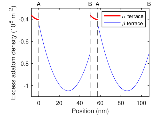
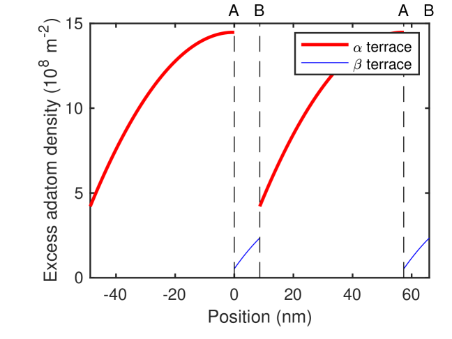
Figures 20 and 21 show the distribution of adatom density on a sequence of $\alpha$ and $\beta$ terraces at steady-state. Since the deviations from $\rho_{eq}^{0}$ are very small, these are shown as the excess density $\rho_{i}-\rho_{eq}^{0}$. In Fig. 20, where $G$ is negative (i.e. evaporation is faster than deposition), the densities tend to go through minima on each terrace, while in Fig. 21, $G$ is positive (i.e. deposition is faster than evaporation), the densities tend to go through maxima. The low values of $\kappa_{-}^{A}$ and $\kappa_{-}^{B}$ used imply large ES barriers at the downhill (positive $y$) edges of the terraces, moving the maximum or minimum to that side. The value of $\kappa_{0}^{B}$ gives significant transport across the $B$ step, reducing difference in adatom densities across the step.

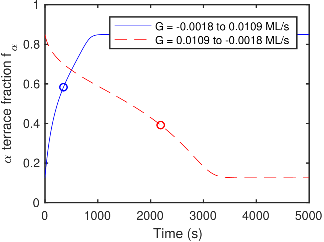
Figure 22 shows the calculated time dependence of $f_{\alpha}$ obtained by integrating the quasi-steady-state result, Eq. (43), for changes between the two conditions of $F=0$ and $F=1.43\times 10^{17}$ m^-2s^-1. While the predicted shapes are not simple exponentials in these cases, for fitting to experiments we nonetheless characterize the model dynamics using the time to reach the $1/e$ fraction of the change in steady-state $f_{\alpha}^{ss}$.

IV.3 Analytical solution for non-transparent steps

Because all four boundary conditions implied by Eq. (30) involve terms in all four coefficients $C_{1i}$ and $C_{2i}$, the explicit analytical solution of Eq. (34) for the coefficients gives very elaborate expressions. In the case of non-transparent steps, with $r_{A}=r_{B}=0$, half of the elements of $\mathcal{M}$ drop out and the boundary conditions split into two sets of two equations, each involving only two coefficients. In this case the analytical solutions are

$$C_{1\alpha} =\frac{-F\tau[2p_{B}q_{A}s_{\alpha}+(p_{B}+q_{A})c_{\alpha}]+(\rho_{eq}^{A}+\rho_{eq}^{B})p_{B}q_{A}s_{\alpha}+(q_{A}\rho_{eq}^{A}+p_{B}\rho_{eq}^{B})c_{\alpha}}{(p_{B}+q_{A})(s_{\alpha}^{2}+c_{\alpha}^{2})+2(1+p_{B}q_{A})s_{\alpha}c_{\alpha}},$$ (46)

$$C_{2\alpha} =\frac{F\tau(p_{B}-q_{A})s_{\alpha}+(\rho_{eq}^{A}-\rho_{eq}^{B})p_{B}q_{A}c_{\alpha}+(q_{A}\rho_{eq}^{A}-p_{B}\rho_{eq}^{B})s_{\alpha}}{(p_{B}+q_{A})(s_{\alpha}^{2}+c_{\alpha}^{2})+2(1+p_{B}q_{A})s_{\alpha}c_{\alpha}},$$ (47)

$$C_{1\beta} =\frac{-F\tau[2p_{A}q_{B}s_{\beta}+(p_{A}+q_{B})c_{\beta}]+(\rho_{eq}^{B}+\rho_{eq}^{A})p_{A}q_{B}s_{\beta}+(q_{B}\rho_{eq}^{B}+p_{A}\rho_{eq}^{A})c_{\beta}}{(p_{A}+q_{B})(s_{\beta}^{2}+c_{\beta}^{2})+2(1+p_{A}q_{B})s_{\beta}c_{\beta}},$$ (48)

$$C_{2\beta} =\frac{F\tau(p_{A}-q_{B})s_{\beta}+(\rho_{eq}^{B}-\rho_{eq}^{A})p_{A}q_{B}c_{\beta}+(q_{B}\rho_{eq}^{B}-p_{A}\rho_{eq}^{A})s_{\beta}}{(p_{A}+q_{B})(s_{\beta}^{2}+c_{\beta}^{2})+2(1+p_{A}q_{B})s_{\beta}c_{\beta}}.$$ (49)

IV.4 Analytical solution for transparent steps

To obtain an analytical solution of Eq. (34) including the effects of step transparency, we can work with an alternative, equivalent formulation of the boundary conditions Pierre-Louis (2003b)

$$J_{\alpha}^{+} =-D\nabla\rho_{\alpha}^{+}=+\tilde{\kappa}_{-}^{A}(\rho_{\alpha}^{+}-\tilde{\rho}_{eq}^{A}),$$ (50)

$$J_{\alpha}^{-} =-D\nabla\rho_{\alpha}^{-}=-\tilde{\kappa}_{+}^{B}(\rho_{\alpha}^{-}-\tilde{\rho}_{eq}^{B}),$$ (51)

$$J_{\beta}^{+} =-D\nabla\rho_{\beta}^{+}=+\tilde{\kappa}_{-}^{B}(\rho_{\beta}^{+}-\tilde{\rho}_{eq}^{B}),$$ (52)

$$J_{\beta}^{-} =-D\nabla\rho_{\beta}^{-}=-\tilde{\kappa}_{+}^{A}(\rho_{\beta}^{-}-\tilde{\rho}_{eq}^{A}),$$ (53)

where the quantities with tildes are defined as

$$\tilde{\kappa}_{+}^{j} \equiv\frac{\langle\kappa^{2}\rangle^{j}}{\kappa_{-}^{j}},$$ (54)

$$\tilde{\kappa}_{-}^{j} \equiv\frac{\langle\kappa^{2}\rangle^{j}}{\kappa_{+}^{j}},$$ (55)

$$\tilde{\rho}_{eq}^{j} \equiv\rho_{eq}^{j}+\frac{v_{j}\rho_{0}\kappa_{0}^{j}}{\langle\kappa^{2}\rangle^{j}},$$ (56)

$$\langle\kappa^{2}\rangle^{j} \equiv\kappa_{+}^{j}\kappa_{-}^{j}+\kappa_{+}^{j}\kappa_{0}^{j}+\kappa_{-}^{j}\kappa_{0}^{j}.$$ (57)

Note that in Eq. (56) the effective equilibrium adatom density $\tilde{\rho}_{eq}^{j}$ at a step of type $j$ depends on the step velocity $v_{j}$. The boundary conditions can be written as

$$\tilde{\mathcal{M}}\mathcal{C}=\tilde{\mathcal{B}},$$ (58)

where $\tilde{\mathcal{M}}$ and $\tilde{\mathcal{B}}$ are given by

$$\tilde{\mathcal{M}}=$$

$$\begin{bmatrix}s_{\alpha}+\tilde{q}_{A}c_{\alpha}&c_{\alpha}+\tilde{q}_{A}s_{\alpha}&0&0\\ s_{\alpha}+\tilde{p}_{B}c_{\alpha}&-c_{\alpha}-\tilde{p}_{B}s_{\alpha}&0&0\\ 0&0&s_{\beta}+\tilde{q}_{B}c_{\beta}&c_{\beta}+\tilde{q}_{B}s_{\beta}\\ 0&0&s_{\beta}+\tilde{p}_{A}c_{\beta}&-c_{\beta}-\tilde{p}_{A}s_{\beta}\end{bmatrix},$$ (59)

$$\tilde{\mathcal{B}}=\begin{bmatrix}\tilde{q}_{A}(\tilde{\rho}_{eq}^{A}-F\tau)\\ \tilde{p}_{B}(\tilde{\rho}_{eq}^{B}-F\tau)\\ \tilde{q}_{B}(\tilde{\rho}_{eq}^{B}-F\tau)\\ \tilde{p}_{A}(\tilde{\rho}_{eq}^{A}-F\tau)\end{bmatrix},$$ (60)

using new dimensionless step kinetic parameters

$$\tilde{p}_{j} \equiv\sqrt{\frac{\tau}{D}}\tilde{\kappa}_{+}^{j}=\frac{p_{j}q_{j}+p_{j}r_{j}+q_{j}r_{j}}{q_{j}},$$ (61)

$$\tilde{q}_{j} \equiv\sqrt{\frac{\tau}{D}}\tilde{\kappa}_{-}^{j}=\frac{p_{j}q_{j}+p_{j}r_{j}+q_{j}r_{j}}{p_{j}},$$ (62)

for step types $j=A$ and $B$. As in the case of non-transparent steps, these boundary conditions consist of two sets of two equations, each involving only two coefficients, $C_{1i}$ and $C_{2i}$ with $i=\alpha$ or $\beta$. The solutions are the same as Eqs. (46-49), with $p_{j}$, $q_{j}$, and $\rho_{eq}^{j}$ replaced by $\tilde{p}_{j}$, $\tilde{q}_{j}$, and $\tilde{\rho}_{eq}^{j}$, respectively. Unfortunately, since the $\tilde{\rho}_{eq}^{j}$ that appear in the $C_{1i}$ and $C_{2i}$ depend upon the step velocities $v_{j}$, which in turn depend upon the $C_{1i}$ and $C_{2i}$ via Eqs. (35-36), this still does not provide an explicit solution for the $C_{1i}$ and $C_{2i}$.

IV.5 Simplified analytical solution

It is very useful to consider some generally applicable limits which simplify the analytical solution, allowing the steady-state terrace fraction and its dynamics to to be expressed in terms of the net growth rate. We start with Eqs. (46-49), with $p_{j}$, $q_{j}$, and $\rho_{eq}^{j}$ replaced by $\tilde{p}_{j}$, $\tilde{q}_{j}$, and $\tilde{\rho}_{eq}^{j}$, respectively. In the limit where the diffusion length within an adatom lifetime is much larger than the terrace widths, $\sqrt{D\tau}>>w$, the coefficients $c_{i}$ can be set equal to unity, and the coefficients $s_{i}$ are small quantities given by $s_{i}=w_{i}/(2\sqrt{D\tau})$. In the limit $\ell_{i}<<w_{i}$, the adatom densities $\rho_{i}$ do not differ much from $\rho_{eq}^{0}$, and thus the adatom evaporation flux is relatively uniform at $\rho_{eq}^{0}/\tau$. Assuming the second term in Eq. (56) is small, we can replace $\tilde{\rho}_{eq}^{A}$ and $\tilde{\rho}_{eq}^{B}$ by $\rho_{eq}^{0}$, except in the difference $(\tilde{\rho}_{eq}^{A}-\tilde{\rho}_{eq}^{B})$. We check the self-consistency of this assumption below. If we also assume that the attachment parameters are generally greater than unity, so that $\tilde{p}_{A}\tilde{q}_{B}>>1$, $\tilde{p}_{B}\tilde{q}_{A}>>1$, the formulas for $C_{1i}$ simplify to be

$$C_{1\alpha}\approx C_{1\beta}\approx\rho_{eq}^{0}-F\tau.$$ (63)

The net growth rate is then simply given by

$$G\approx\frac{F-\rho_{eq}^{0}/\tau}{\rho_{0}},$$ (64)

which is the difference between the deposition flux $F$ and a uniform evaporation flux $\rho_{eq}^{0}/\tau$, converted to ML/s using $\rho_{0}$. We can write the expressions for the $C_{2i}$ as

$$C_{2\alpha} \approx\frac{\sqrt{D\tau}}{w}\big{[}R_{\alpha}(\tilde{\rho}_{eq}^{A}-\tilde{\rho}_{eq}^{B})+S_{\alpha}\rho_{0}G\big{]},$$ (65)

$$C_{2\beta} \approx\frac{\sqrt{D\tau}}{w}\big{[}R_{\beta}(\tilde{\rho}_{eq}^{B}-\tilde{\rho}_{eq}^{A})+S_{\beta}\rho_{0}G\big{]},$$ (66)

where each contains a term that is proportional to the net growth rate $G$. The coefficients are give by

$$R_{\alpha} \equiv\frac{w}{D}\left(\frac{\kappa_{+}^{A}}{\langle\kappa^{2}\rangle^{A}}+\frac{\kappa_{-}^{B}}{\langle\kappa^{2}\rangle^{B}}+\frac{wf_{\alpha}}{D}\right)^{-1},$$ (67)

$$R_{\beta} \equiv\frac{w}{D}\left(\frac{\kappa_{+}^{B}}{\langle\kappa^{2}\rangle^{B}}+\frac{\kappa_{-}^{A}}{\langle\kappa^{2}\rangle^{A}}+\frac{w(1-f_{\alpha})}{D}\right)^{-1},$$ (68)

$$S_{\alpha} \equiv\frac{R_{\alpha}wf_{\alpha}}{2}\left(\frac{\kappa_{+}^{A}}{\langle\kappa^{2}\rangle^{A}}-\frac{\kappa_{-}^{B}}{\langle\kappa^{2}\rangle^{B}}\right),$$ (69)

$$S_{\beta} \equiv\frac{R_{\beta}w(1-f_{\alpha})}{2}\left(\frac{\kappa_{+}^{B}}{\langle\kappa^{2}\rangle^{B}}-\frac{\kappa_{-}^{A}}{\langle\kappa^{2}\rangle^{A}}\right),$$ (70)

where the $R_{i}$ are positive and dimensionless and the $S_{i}$ have dimensions of time. The step velocities of Eqs. (35-36) become

$$v_{A} =\frac{wG}{2}+\frac{D}{\rho_{0}w}\big{[}(R_{\alpha}+R_{\beta})(\tilde{\rho}_{eq}^{B}-\tilde{\rho}_{eq}^{A})+(S_{\beta}-S_{\alpha})\rho_{0}G\big{]},$$ (71)

$$v_{B} =\frac{wG}{2}+\frac{D}{\rho_{0}w}\big{[}(R_{\alpha}+R_{\beta})(\tilde{\rho}_{eq}^{A}-\tilde{\rho}_{eq}^{B})+(S_{\alpha}-S_{\beta})\rho_{0}G\big{]}.$$ (72)

The difference of the effective equilibrium step adatom densities also contains a term that is proportional to $G$,

$$\tilde{\rho}_{eq}^{A}-\tilde{\rho}_{eq}^{B}=\frac{2\rho_{eq}^{0}\mathbf{M}+\rho_{0}G\big{[}S_{0}+R_{0}(S_{\beta}-S_{\alpha})\big{]}}{1+R_{0}(R_{\alpha}+R_{\beta})},$$ (73)

where the new coefficients are given by

$$R_{0} \equiv\frac{D}{w}\left(\frac{\kappa_{0}^{A}}{\langle\kappa^{2}\rangle^{A}}+\frac{\kappa_{0}^{B}}{\langle\kappa^{2}\rangle^{B}}\right),$$ (74)

$$S_{0} \equiv\frac{w}{2}\left(\frac{\kappa_{0}^{A}}{\langle\kappa^{2}\rangle^{A}}-\frac{\kappa_{0}^{B}}{\langle\kappa^{2}\rangle^{B}}\right).$$ (75)

The rate of change of $f_{\alpha}$ becomes

$$\frac{df_{\alpha}}{dt}=\mathbf{K}^{dyn}(f_{\alpha})\left(\frac{G}{\mathbf{K}^{ss}(f_{\alpha})}-\frac{4\mathbf{M}(f_{\alpha})\rho_{eq}^{0}}{w\rho_{0}}\right),$$ (76)

where we have introduced the combined kinetic coefficient functions $\mathbf{K}^{ss}(f_{\alpha})$ and $\mathbf{K}^{dyn}(f_{\alpha})$, defined by

$$\mathbf{K}^{ss}(f_{\alpha}) \equiv\frac{w}{2\big{[}-S_{0}+(S_{\beta}-S_{\alpha})/(R_{\alpha}+R_{\beta})\big{]}},$$ (77)

$$\mathbf{K}^{dyn}(f_{\alpha}) \equiv\frac{D(R_{\alpha}+R_{\beta})}{w[1+R_{0}(R_{\alpha}+R_{\beta})]}.$$ (78)

These functions have the same dimensions as the individual $\kappa_{x}^{j}$ coefficients (length/time). $\mathbf{K}^{dyn}(f_{\alpha})$ is always positive; $\mathbf{K}^{ss}(f_{\alpha})$ depends on the differences in the $\kappa_{x}^{j}$, such that in the limit where all $\kappa_{x}^{j}$ are equal, $\mathbf{K}^{ss}\rightarrow\infty$. In this case the influence of $G$ on $f_{\alpha}$ becomes negligible, and the steady-state $\alpha$ terrace fraction is always $f_{\alpha}^{ss}=f_{\alpha}^{0}$ (i.e. the value where $\mathbf{M}=0$), independent of $G$.

The general equation to obtain the full steady state is

$$G^{ss}(f_{\alpha})=\frac{4\,\mathbf{K}^{ss}(f_{\alpha})\,\mathbf{M}(f_{\alpha})\rho_{eq}^{0}}{w\rho_{0}}.$$ (79)

This equation for $G^{ss}(f_{\alpha})$ can be inverted to obtain a master curve for the steady-state value $f_{\alpha}^{ss}$ as a function of $G$. For both the dynamics Eq. (76) and the steady-state Eq. (79), the six step attachment parameters enter through the six combinations in the coefficients $R_{i}$, $S_{i}$, $R_{0}$, and $S_{0}$. The only dependence on $\tau$ and $F$ is through their combination into $G$, Eq. (64).

The curve $G^{ss}(f_{\alpha})$ always passes through $G=0$ at $f_{\alpha}=f_{\alpha}^{0}$, since $\mathbf{M}$ is zero there. The slope of the curve at $f_{\alpha}=f_{\alpha}^{0}$ is given by

$$G^{*} \equiv\left.\frac{dG^{ss}}{df_{\alpha}}\right|_{f_{\alpha}^{0}}=\frac{4\,\mathbf{K}^{ss}(f_{\alpha}^{0})\rho_{eq}^{0}}{w\rho_{0}}\left.\frac{d\mathbf{M}}{df_{\alpha}}\right|_{f_{\alpha}^{0}}$$

$$=\frac{12\rho_{eq}^{0}\ell^{3}\mathbf{K}^{ss}(f_{\alpha}^{0})}{\rho_{0}w^{4}f_{\alpha}^{0}(1-f_{\alpha}^{0})}.$$ (80)

The sign of the slope of $G^{ss}(f_{\alpha})$, and thus $f_{\alpha}^{ss}(G)$, is determined by the sign of $\mathbf{K}^{ss}(f_{\alpha}^{0})$.

One can see that $f_{\alpha}$ is always stable to a small perturbation from steady state $\Delta f_{\alpha}\equiv f_{\alpha}-f_{\alpha}^{ss}(G)$ by writing Eq. (76) as

$$\frac{df_{\alpha}}{dt}=\frac{\mathbf{K}^{dyn}(f_{\alpha})}{\mathbf{K}^{ss}(f_{\alpha})}\big{[}G-G^{ss}(f_{\alpha})\big{]}.$$ (81)

For example, when $\mathbf{K}^{ss}$ is positive, and $\Delta f_{\alpha}$ is positive, then $G-G^{ss}(f_{\alpha})$ will be negative, and the perturbation will decay. For $f_{\alpha}$ near $f_{\alpha}^{0}$, the relaxation time $t^{*}$ of the perturbation can be obtained using $G-G^{ss}(f_{\alpha})\approx-G^{*}\Delta f_{\alpha}$, giving

$$\frac{1}{t^{*}}\equiv\frac{-1}{\Delta f_{\alpha}}\frac{df_{\alpha}}{dt}\approx\frac{\mathbf{K}^{dyn}\,G^{*}}{\mathbf{K}^{ss}}=\frac{12\rho_{eq}^{0}\ell^{3}\mathbf{K}^{dyn}}{\rho_{0}w^{4}f_{\alpha}^{0}(1-f_{\alpha}^{0})}.$$ (82)

To check the self-consistency of the assumption that the $\tilde{\rho}_{eq}^{j}$ do not differ much from $\rho_{eq}^{0}$, used to obtain the simplified analytical solution, we require that the second term in Eq. (56) is negligible with respect to $\rho_{eq}^{0}$, or

$$\left|\frac{v_{j}\rho_{0}\kappa_{0}^{j}}{\langle\kappa^{2}\rangle^{j}}\right|<<\rho_{eq}^{0}$$ (83)

for both steps $j=A$ and $B$. We can write the expressions for the step velocities Eqs. (71,72) as

$$v_{A} =\frac{wG}{2}+\frac{2\,\mathbf{M}\,\mathbf{K}^{dyn}\rho_{eq}^{0}}{\rho_{0}}\left[\frac{G-G^{ss}}{G^{ss}}\right],$$ (84)

$$v_{B} =\frac{wG}{2}-\frac{2\,\mathbf{M}\,\mathbf{K}^{dyn}\rho_{eq}^{0}}{\rho_{0}}\left[\frac{G-G^{ss}}{G^{ss}}\right].$$ (85)

The first term gives the steady-state velocity, and the second term gives the difference in velocity when $f_{\alpha}$ differs from $f_{\alpha}^{ss}$. For the steady-state term, relation (83) gives maximum growth rate magnitudes of

$$|G|<<\frac{2\rho_{eq}^{0}\langle\kappa^{2}\rangle^{j}}{w\rho_{0}\kappa_{0}^{j}}$$ (86)

for both steps $j=A$ and $B$. For the dynamic term, relation (83) gives maximum growth rate difference magnitudes of

$$|G-G^{ss}|<<\left|\frac{w\rho_{0}[1+R_{0}(R_{\alpha}+R_{\beta})]G^{ss}\langle\kappa^{2}\rangle^{j}}{2D\mathbf{M}\rho_{eq}^{0}(R_{\alpha}+R_{\beta})\kappa_{0}^{j}}\right|.$$ (87)

For the parameter ranges we consider, these limits on growth rate are many orders of magnitude larger than the growth rates relevant to this study, confirming the validity of the simplified analytical solution. We have also checked that the exact solution obtained using the matrix equations Eqs. (30-34) agrees with the simplified analytical solution.

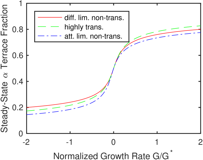
Figure 23 shows the some examples of $f_{\alpha}^{ss}$ vs. $G/G^{*}$, calculated using the simplified analytical solution Eqs. (77-80) with parameter values given in Table 3. These correspond to some of the limiting cases discussed below.

Figure 23: Master curves of $f_{\alpha}^{ss}$ vs. $G/G^{*}$ for 3 cases: diffusion-limited kinetics with non-transparent steps, attachment-limited kinetics with non-transparent steps, and either kinetics with highly transparent steps. Parameter values used are given in Table 3.

Table 3: Parameter values used in BCF theory calculations for four sub-cases shown in Fig. 23. All used $w=5.73\times 10^{-8}$ m, $\rho_{0}=1.13\times 10^{19}$ m^-2, $\ell=9\times 10^{-10}$ m, $\rho_{eq}^{0}=3.4\times 10^{11}$ m^-2, $f_{\alpha}^{0}$ = 0.5.

Kinetics limited by:	diff.	diff.	attach.	attach.
Step transparency:	zero	high	zero	high
$D$     (m2/s)	$10^{-14}$	$10^{-14}$	$10^{-4}$	$10^{-4}$
$\kappa_{+}^{A}$    (m/s)	$10^{2}$	$10^{2}$	$10^{2}$	$10^{2}$
$\kappa_{-}^{A}$    (m/s)	$10^{1}$	$10^{1}$	$10^{1}$	$10^{1}$
$\kappa_{0}^{A}$    (m/s)	$0$	$10^{3}$	$0$	$10^{3}$
$\kappa_{+}^{B}$    (m/s)	$10^{1}$	$10^{1}$	$10^{1}$	$10^{1}$
$\kappa_{-}^{B}$    (m/s)	$10^{0}$	$10^{0}$	$10^{0}$	$10^{0}$
$\kappa_{0}^{B}$    (m/s)	$0$	$10^{3}$	$0$	$10^{3}$
$G^{*}$    (10-3 ML/s)	$0.4$	$1.2$	$1.2$	$1.2$

We next use the simplified analytical solution to consider two cases, in which the adatom kinetics on the terraces are limited by diffusion or by attachment/detachment at steps Guin et al. (2020). For each, we consider the sub-cases of non-transparent or highly transparent steps, and examine the factors that determine the sign of $\mathbf{K}^{ss}$, and thus whether $f_{\alpha}^{ss}(G)$ has a positive or negative slope. We finally consider a third case in which $\alpha$ and $\beta$ terraces have different limiting kinetics.

IV.6 Diffusion-limited kinetics

In the diffusion-limited case, the first two terms are negligible in Eq. (67) for $R_{\alpha}$ and in Eq. (68) for $R_{\beta}$. These expressions reduce to $R_{\alpha}=f_{\alpha}^{-1}$ and $R_{\beta}=(1-f_{\alpha})^{-1}$. The coefficients $S_{\alpha}$ and $S_{\beta}$ become independent of $f_{\alpha}$. The expression for $\mathbf{K}^{ss}$ is given by

$$\mathbf{K}^{ss}(f_{\alpha})\approx\big{[}W_{0}^{dl}+W_{1}^{dl}f_{\alpha}(1-f_{\alpha})\big{]}^{-1},$$ (88)

where we have introduced coefficients

$$W_{0}^{dl} \equiv\frac{\kappa_{0}^{B}}{\langle\kappa^{2}\rangle^{B}}-\frac{\kappa_{0}^{A}}{\langle\kappa^{2}\rangle^{A}},$$ (89)

$$W_{1}^{dl} \equiv\frac{\kappa_{+}^{B}}{\langle\kappa^{2}\rangle^{B}}+\frac{\kappa_{-}^{B}}{\langle\kappa^{2}\rangle^{B}}-\frac{\kappa_{+}^{A}}{\langle\kappa^{2}\rangle^{A}}-\frac{\kappa_{-}^{A}}{\langle\kappa^{2}\rangle^{A}}.$$ (90)

The expression for $\mathbf{K}^{dyn}$ becomes

$$\mathbf{K}^{dyn}\approx\frac{D}{w[f_{\alpha}(1-f_{\alpha})+R_{0}]}.$$ (91)

For the sub-case of non-transparent steps, with $\kappa_{0}^{A}=\kappa_{0}^{B}=0$, we have $\langle\kappa^{2}\rangle^{j}=\kappa_{+}^{j}\kappa_{-}^{j}$ for both steps $j=A$ and $B$. The expression for $\mathbf{K}^{ss}$ becomes

$$\mathbf{K}^{ss}(f_{\alpha})\approx\left[f_{\alpha}(1-f_{\alpha})\left(\frac{1}{\kappa_{-}^{B}}+\frac{1}{\kappa_{+}^{B}}-\frac{1}{\kappa_{-}^{A}}-\frac{1}{\kappa_{+}^{A}}\right)\right]^{-1}.$$ (92)

Here the smallest of the individual $\kappa_{+}^{j}$ or $\kappa_{-}^{j}$ tends to dominate and determine the sign of $\mathbf{K}^{ss}$. The sign of $\mathbf{K}^{ss}$ is positive if the smallest coefficient is for the $B$ step, e.g. if the $B$ step has the higher ES barrier, so that $\kappa_{-}^{B}$ is smallest. If there are no ES barriers, i.e. $\kappa_{-}^{j}=\kappa_{+}^{j}$, then the step with the smaller $\kappa_{+}^{j}$ determines the sign. In this sub-case we have $R_{0}=0$, which simplifies Eq. (91) for $df_{\alpha}/dt$.

For the sub-case of highly transparent steps, with $\kappa_{0}^{j}>>\kappa_{+}^{j}$ and $\kappa_{-}^{j}$, we have $\langle\kappa^{2}\rangle^{j}=\kappa_{0}^{j}(\kappa_{+}^{j}+\kappa_{-}^{j})$ for both steps $j=A$ and $B$. The expression for $\mathbf{K}^{ss}$ becomes a constant, independent of $f_{\alpha}$,

$$\mathbf{K}^{ss}\approx\left(\frac{1}{\kappa_{-}^{B}+\kappa_{+}^{B}}-\frac{1}{\kappa_{-}^{A}+\kappa_{+}^{A}}\right)^{-1}.$$ (93)

Here the behavior just depends on the sums $\kappa_{-}^{j}+\kappa_{+}^{j}$ for each step. It does not matter whether there are ES barriers; the sign of $\mathbf{K}^{ss}$ is positive if $(\kappa_{-}^{A}+\kappa_{+}^{A})>(\kappa_{-}^{B}+\kappa_{+}^{B})$.

IV.7 Attachment-limited kinetics

In the attachment-limited case, the final term is negligible in Eq. (67) for $R_{\alpha}$ and in Eq. (68) for $R_{\beta}$. The coefficients $R_{\alpha}$ and $R_{\beta}$ become independent of $f_{\alpha}$. The expression for $\mathbf{K}^{ss}$ is given by

$$\mathbf{K}^{ss}(f_{\alpha})\approx\big{[}W_{0}^{al}+W_{1}^{al}(1-2f_{\alpha})\big{]}^{-1},$$ (94)

with coefficients

$$W_{0}^{al} \equiv\frac{\langle\kappa^{2}\rangle^{A}-\langle\kappa^{2}\rangle^{B}+(\kappa_{+}^{A}+\kappa_{-}^{A})\kappa_{0}^{B}-(\kappa_{+}^{B}+\kappa_{-}^{B})\kappa_{0}^{A}}{(\kappa_{+}^{B}+\kappa_{-}^{B})\langle\kappa^{2}\rangle^{A}+(\kappa_{+}^{A}+\kappa_{-}^{A})\langle\kappa^{2}\rangle^{B}},$$ (95)

$$W_{1}^{al} \equiv\frac{\kappa_{+}^{B}\kappa_{+}^{A}-\kappa_{-}^{B}\kappa_{-}^{A}}{(\kappa_{+}^{B}+\kappa_{-}^{B})\langle\kappa^{2}\rangle^{A}+(\kappa_{+}^{A}+\kappa_{-}^{A})\langle\kappa^{2}\rangle^{B}}.$$ (96)

The expression for $\mathbf{K}^{dyn}$ is independent of $f_{\alpha}$,

$$\mathbf{K}^{dyn}\approx\left(\left[\left(\frac{\kappa_{+}^{B}}{\langle\kappa^{2}\rangle^{B}}+\frac{\kappa_{-}^{A}}{\langle\kappa^{2}\rangle^{A}}\right)^{-1}\right.\right.$$

$$+\left.\left.\left(\frac{\kappa_{-}^{B}}{\langle\kappa^{2}\rangle^{B}}+\frac{\kappa_{+}^{A}}{\langle\kappa^{2}\rangle^{A}}\right)^{-1}\right]^{-1}+\frac{\kappa_{0}^{A}}{\langle\kappa^{2}\rangle^{A}}+\frac{\kappa_{0}^{B}}{\langle\kappa^{2}\rangle^{B}}\right)^{-1}.$$ (97)

The diffusion coefficient $D$ does not enter into the solution for the attachment-limited case; its role in the dynamics is taken by the combination of all the $\kappa$ coefficients given in Eq. (97). Since the denominators in Eqs. (95-96) are always positive, the sign of $\mathbf{K}^{ss}$ is determined by the numerators.

For the sub-case of non-transparent steps, with $\kappa_{0}^{A}=\kappa_{0}^{B}=0$, $\langle\kappa^{2}\rangle^{j}=\kappa_{+}^{j}\kappa_{-}^{j}$, the expressions for the coefficients in $\mathbf{K}^{ss}$ become

$$W_{0}^{al} \equiv\frac{\kappa_{+}^{A}\kappa_{-}^{A}-\kappa_{+}^{B}\kappa_{-}^{B}}{(\kappa_{+}^{B}+\kappa_{-}^{B})\kappa_{+}^{A}\kappa_{-}^{A}+(\kappa_{+}^{A}+\kappa_{-}^{A})\kappa_{+}^{B}\kappa_{-}^{B}},$$ (98)

$$W_{1}^{al} \equiv\frac{\kappa_{+}^{B}\kappa_{+}^{A}-\kappa_{-}^{B}\kappa_{-}^{A}}{(\kappa_{+}^{B}+\kappa_{-}^{B})\kappa_{+}^{A}\kappa_{-}^{A}+(\kappa_{+}^{A}+\kappa_{-}^{A})\kappa_{+}^{B}\kappa_{-}^{B}}.$$ (99)

This is the most complex sub-case. Near $f_{\alpha}=0.5$, the sign of $\mathbf{K}^{ss}$ is positive if $\kappa_{+}^{B}\kappa_{-}^{B}<\kappa_{+}^{A}\kappa_{-}^{A}$. At $f_{\alpha}>0.5$, if the steps have normal ES barriers with $\kappa_{-}^{j}<\kappa_{+}^{j}$, the $W_{1}^{al}$ term will favor a negative sign. Thus the sign of $\mathbf{K}^{ss}$ can change with $f_{\alpha}$. The expression for $\mathbf{K}^{dyn}$ becomes

$$\mathbf{K}^{dyn}\approx\left(\frac{1}{\kappa_{-}^{B}}+\frac{1}{\kappa_{+}^{A}}\right)^{-1}+\left(\frac{1}{\kappa_{+}^{B}}+\frac{1}{\kappa_{-}^{A}}\right)^{-1}.$$ (100)

The dynamic coefficient has an interesting form, dominated by the terrace with the largest value of the smallest attachment coefficient at its edges.

For the sub-case of highly transparent steps, with $\kappa_{0}^{j}>>\kappa_{+}^{j}$ and $\kappa_{-}^{j}$, $\langle\kappa^{2}\rangle^{j}=\kappa_{0}^{j}(\kappa_{+}^{j}+\kappa_{-}^{j})$, the expression for $\mathbf{K}^{ss}$ becomes a constant identical to that for diffusion-limited kinetics with highly transparent steps,

$$\mathbf{K}^{ss}\approx\left(\frac{1}{\kappa_{-}^{B}+\kappa_{+}^{B}}-\frac{1}{\kappa_{-}^{A}+\kappa_{+}^{A}}\right)^{-1}.$$ (101)

As before, the steady-state behavior just depends on the sums $\kappa_{-}^{j}+\kappa_{+}^{j}$ for each step. The dynamics still differs from the diffusion-limited case, since the expression for $\mathbf{K}^{dyn}$ differs from Eq. (91),

$$\mathbf{K}^{dyn}\approx\left(\frac{1}{\kappa_{-}^{B}+\kappa_{+}^{B}}+\frac{1}{\kappa_{-}^{A}+\kappa_{+}^{A}}\right)^{-1}.$$ (102)

IV.8 Mixed kinetics

The limits considered above assume that both terraces have the same kinetics, either diffusion- or attachment-limited, and that both steps have the same transparency, either zero or high. Because the attachment coefficients can be different for each step type, other limiting cases are possible. Here we consider the limit in which the $\kappa_{+}^{A}$ coefficient is much larger than the other five $\kappa_{x}^{j}$, so that the $A$ step has a high ES barrier, with $\kappa_{-}^{A}+\kappa_{0}^{A}<<D/wf_{\alpha}$ (the $A$ step is non-transparent). We also assume that $\kappa_{-}^{B}<<\kappa_{+}^{B}\kappa_{0}^{B}/(\kappa_{+}^{B}+\kappa_{0}^{B})$ so that the $B$ step also has a high ES barrier. In this case we have $\langle\kappa^{2}\rangle^{A}=\kappa_{+}^{A}(\kappa_{-}^{A}+\kappa_{0}^{A})$ and $\langle\kappa^{2}\rangle^{B}=\kappa_{+}^{B}\kappa_{0}^{B}$. The second and third terms in Eq. (67) are negligible, giving $R_{\alpha}=(w/D)(\kappa_{-}^{A}+\kappa_{0}^{A})$. The second term in Eq. (68) is negligible, giving $R_{\beta}=[D/(w\kappa_{0}^{B})+(1-f_{\alpha})]^{-1}$. The second terms in Eqs. (69) and (70) are negligible, giving $S_{\alpha}=w^{2}f_{\alpha}/(2D)$, $S_{\beta}=(w/2)(1-f_{\alpha})/[D/w+(1-f_{\alpha})\kappa_{0}^{B}]$. The first terms in Eqs. (74) and (75) are negligible, giving $R_{0}=D/(w\kappa_{+}^{B})$, $S_{0}=-w/(2\kappa_{+}^{B})$. This results in expressions

$$\mathbf{K}^{ss}(f_{\alpha})\approx\left[\frac{1}{\kappa_{+}^{B}}+\frac{(1-2f_{\alpha})}{\kappa_{0}^{B}}-\frac{wf_{\alpha}(1-f_{\alpha})}{D}\right]^{-1},$$ (103)

$$\frac{df_{\alpha}}{dt}\approx\left[\frac{D}{\kappa_{+}^{B}}+\frac{D}{\kappa_{0}^{B}}+w(1-f_{\alpha})\right]^{-1}\times$$

$$\left(G\left[\frac{D}{\kappa_{+}^{B}}+\frac{D(1-2f_{\alpha})}{\kappa_{0}^{B}}-wf_{\alpha}(1-f_{\alpha})\right]-\right.$$

$$\left.\frac{4D\rho_{eq}^{0}}{w\rho_{0}}\left(\frac{\ell}{w}\right)^{3}\left[\left(\frac{1-f_{\alpha}^{0}}{1-f_{\alpha}}\right)^{3}-\left(\frac{f_{\alpha}^{0}}{f_{\alpha}}\right)^{3}\right]\right),$$ (104)

$$G^{ss}\approx\frac{4D\rho_{eq}^{0}}{w\rho_{0}}\left(\frac{\ell}{w}\right)^{3}\left[\left(\frac{1-f_{\alpha}^{0}}{1-f_{\alpha}}\right)^{3}-\left(\frac{f_{\alpha}^{0}}{f_{\alpha}}\right)^{3}\right]\times$$

$$\left[\frac{D}{\kappa_{+}^{B}}+\frac{D(1-2f_{\alpha})}{\kappa_{0}^{B}}-wf_{\alpha}(1-f_{\alpha})\right]^{-1}.$$ (105)

Even though $\kappa_{+}^{A}$ has the largest value, the sign of $\mathbf{K}^{ss}$ can be negative depending upon the relative size of the terms in Eq. (103). It will be negative near $f_{\alpha}=0.5$ for $D/\kappa_{+}^{B}<w/4$. If $\kappa_{0}^{B}$ is small, it can become negative for $f_{\alpha}>0.5$.

V Comparison of BCF theory to X-ray measurements

The BCF model predicts the dependence of the steady-state terrace fraction on growth rate $f_{\alpha}^{ss}(G)$, as well as the dynamics of the transitions when $G$ is changed. We can compare calculated values to our measurements to understand the implications for the physics in the model, such as the differences between adatom attachment kinetics at $A$ and $B$ steps.

In the general model, e.g. Eqs. (58)-(62), there are 14 fundamental variables ($F$, $\tau$, $\rho_{0}$, $w$, $D$, $\rho_{eq}^{0}$, $\ell$, $f_{\alpha}^{0}$, and the six $\kappa_{x}^{j}$). In the simplified analytical solution presented in Section IV.D., four variables enter only through two combinations ($G=F-\rho_{eq}^{0}/\tau$, and $\rho_{eq}^{0}\ell^{3}$), leaving 12 independent variables. We control or directly determine $G$, $\rho_{0}$, and $w$, leaving 9 unknown quantities ($D$, $\rho_{eq}^{0}\ell^{3}$, $f_{\alpha}^{0}$, and the six combinations of the $\kappa_{x}^{j}$) to be determined or constrained by the measurements. This is a challenge because we have only 6 measured quantities (four steady-state $\alpha$ terrace fractions $f_{\alpha}^{ss}$ at different growth rates $G$, and two relaxation times for transitions in $G$.)

As we have seen, in some limits the number of effective parameters is smaller, since only certain combinations of $D$ and the $\kappa_{x}^{j}$ enter the solutions. The diffusion-limited kinetics solutions reduce these 7 to 4 combinations, leaving a total of 6 unknown quantities. The sub-cases of non-transparent or highly transparent steps reduce the number of effective parameters by one or two more. The attachment-limited kinetics solutions reduce these 7 to 2 combinations, leaving a total of 4 unknown quantities. The highly transparent sub-case reduces this by one. The mixed kinetics solution has a total of 4 unknown quantities, $D/\kappa_{+}^{B}$, $D/\kappa_{0}^{B}$, $D\rho_{eq}^{0}\ell^{3}$, and $f_{\alpha}^{0}$.

To calculate BCF model results to compare with the experimental conditions, we assume that the only parameter affected by the TEGa supply rate is the deposition flux $F$, and that the only parameter affected by the carrier gas composition (0% or 50% H₂) is the adatom lifetime $\tau$, and that these enter only through the net growth rates $G$ given in Table 4 for each condition, as determined in Appendix C. We use the known values $\rho_{0}=2a^{-2}/\sqrt{3}=1.13\times 10^{19}$ m^-2 and $w=c/\sin(0.52^{\circ})=5.73\times 10^{-8}$ m, where $a=3.20\times 10^{-10}$ m and $c=5.20\times 10^{-10}$ m are the lattice parameters of GaN at the growth temperature Reeber and Wang (2000).

Table 4: Comparison of measured values to best fit calculated from the simplified analytical solution of the BCF model, using parameters given in Table 5.

Cond./	$G$		Measured	Best
Trans.	(ML/s)		Value	Fit
$1$	-0.0018	$f_{\alpha}^{ss}$	$0.111\pm 0.013$	$0.136$
$2$	0.0000	$f_{\alpha}^{ss}$	$0.461\pm 0.018$	$0.440$
$3$	0.0109	$f_{\alpha}^{ss}$	$0.811\pm 0.014$	$0.836$
$4$	0.0127	$f_{\alpha}^{ss}$	$0.867\pm 0.011$	$0.847$
$1$ to $2$		$t_{rel}$	$2177\pm 218$ s	$2478$
$2$ to $4$		$t_{rel}$	$341\pm 34$ s	$331$
		$\chi^{2}$	$-$	13.6

Table 5: Parameter values used in simplified analytical BCF model calculations given in Table 4.

Parameter	Best-fit	Best-fit	Units
	Solution #1	Solution #2
$D$	$1.00\times 10^{-4}$	$1.00\times 10^{-9}$	(m2/s)
$\kappa_{+}^{A}$	(large)	(large)	(m/s)
$\kappa_{+}^{B}$	$5.27\times 10^{3}$	$5.27\times 10^{-2}$	(m/s)
$\kappa_{-}^{A}$	$\approx 0$	$\approx 0$	(m/s)
$\kappa_{-}^{B}$	$\approx 0$	$\approx 0$	(m/s)
$\kappa_{0}^{A}$	$\approx 0$	$\approx 0$	(m/s)
$\kappa_{0}^{B}$	$9.45\times 10^{3}$	$9.45\times 10^{-2}$	(m/s)
$\rho_{eq}^{0}\ell^{3}$	$3.31\times 10^{-19}$	$3.31\times 10^{-14}$	(m)
$f_{\alpha}^{0}$	$0.440$	$0.440$	$-$

We searched the space of the 9 unknown quantities of the simplified analytical solution to find the best fit to the measured quantities. Table 4 compares the six measured quantities (four steady-state values of $f_{\alpha}^{ss}$ and two relaxation times $t_{rel}$ following growth rate transitions) to the best-fit values calculated from the BCF model. The best fit was determined by minimizing the goodness-of-fit parameter $\chi^{2}\equiv\sum[(y_{i}-y_{i}^{calc})/\sigma_{i}]^{2}$, where the $y_{i}$ and $\sigma_{i}$ are the six measured quantities and their uncertainties. To estimate the uncertainties in the $f_{\alpha}^{ss}$, we multiplied those obtained in the fits to the 3H(T1) reconstruction by a factor of 4, to account for the uncertainties in the atomic coordinates used. We estimated the uncertainty in the $t_{rel}$ to be 10%. We found a family of equivalent solutions giving essentially the same results and the same minimum $\chi^{2}$. Two examples with different parameter value sets, denoted #1 and #2, are shown in Table 5. For this region of parameter space, the values of several of the parameters could be varied with no significant effect, as long as they were sufficiently large or close to zero, as indicated in Table 5. These best-fit solutions to the simplified analytical model correspond to the mixed kinetics limit described above.

Table 6: Comparison of measured values to those calculated from limiting cases of the BCF model, using parameters given in Table 7.

Cond./	$G$		Measured	Diff.	Attach.	Mixed
Trans.	(ML/s)		Value	Ltd.	Ltd.	Kin.
$1$	-0.0018	$f_{\alpha}^{ss}$	$0.111\pm 0.013$	$0.159$	$0.154$	$0.136$
$2$	0.0000	$f_{\alpha}^{ss}$	$0.461\pm 0.018$	$0.389$	$0.410$	$0.440$
$3$	0.0109	$f_{\alpha}^{ss}$	$0.811\pm 0.014$	$0.863$	$0.830$	$0.836$
$4$	0.0127	$f_{\alpha}^{ss}$	$0.867\pm 0.011$	$0.871$	$0.838$	$0.847$
$1$ to $2$		$t_{rel}$	$2177\pm 218$ s	$2204$	$2958$	$2478$
$2$ to $4$		$t_{rel}$	$341\pm 34$ s	$337$	$251$	$331$
		$\chi^{2}$	$-$	42.5	46.7	13.6

Table 7: Best-fit parameter values for the three limiting cases of the BCF model, for fits shown in Table 6 and Fig. 16.

Diffusion-limited kinetics

Parameter	Value	Units
$DW_{0}^{dl}$	$2.29\times 10^{-9}$	(m)
$DW_{1}^{dl}$	$-5.27\times 10^{-9}$	(m)
$D\rho_{eq}^{0}\ell^{3}$	$6.18\times 10^{-24}$	(m3/s)
$f_{\alpha}^{0}$	$0.389$	$-$

Attachment-limited kinetics

Parameter	Value	Units
$\mathbf{K}^{dyn}W_{0}^{al}$	$9.46\times 10^{-2}$	$-$
$\mathbf{K}^{dyn}W_{1}^{al}$	$6.30\times 10^{-2}$	$-$
$\mathbf{K}^{dyn}\rho_{eq}^{0}\ell^{3}$	$4.17\times 10^{-16}$	(m2/s)
$f_{\alpha}^{0}$	$0.410$	$-$

Mixed kinetics

Parameter	Value	Units
$D/\kappa_{+}^{B}$	$1.90\times 10^{-8}$	(m)
$D/\kappa_{0}^{B}$	$1.06\times 10^{-8}$	(m)
$D\rho_{eq}^{0}\ell^{3}$	$3.31\times 10^{-23}$	(m3/s)
$f_{\alpha}^{0}$	$0.440$	$-$

To understand how well the measurements constrain the model parameters and the physics underlying them, we have also searched for the best fit for each of the three limiting cases. For the diffusion-limited case, the best fit occurs with the parameter $R_{0}$ negligible in Eq. (91), so that only four combinations of unknown quantities are needed to specify the solution, as in the attachment-limited and mixed kinetics cases. Table 6 compares the results of these fits, and Table 7 summarizes the best-fit values of the four quantities obtained for each limiting case. We have also plotted the curves of $f_{\alpha}^{ss}(G)$ corresponding to these fits with the experimental points in Fig. 16. It is clear that the mixed kinetics limit gives a significantly better fit.

To interpret the combined parameters obtained from the fits, it is useful to estimate the adatom diffusivity $D$ and equilibrium adatom density $\rho_{eq}^{0}$. Ab initio calculations of the activation energy for Ga diffusion on the Ga-terminated (0001) surface have given values of $\Delta H_{m}=0.4$ eV Zywietz et al. (1998) and $\Delta H_{m}=0.5$ eV Chugh and Ranganathan (2017b), and similar values have been obtained for 3d transition metal adatoms González-Hernández et al. (2011). An estimate based on spatial correlations in the surface morphology of GaN films grown at two temperatures gave $\Delta H_{m}=1.6\pm 0.5$ eV Koleske et al. (2014). If we estimate the diffusivity from the ab initio calculations using $D=a^{2}\nu\exp(\Delta S_{m}/k)\exp(-\Delta H_{m}/kT)$ Shewmon (1989), with $a=3.2\times 10^{-10}$ m, $\nu=10^{14}$ s^-1, $\Delta S_{m}=0$, and $\Delta H_{m}=0.4$ eV, we obtain $D=1.4\times 10^{-7}$ m²/s at $T=1073$ K. In addition, the surface morphology analysis Koleske et al. (2014) indicated a cross-over at $T=1073$ K from surface diffusion transport to evaporation/condensation transport at a length scale of $\lambda=1.5\times 10^{-6}$ m for OMVPE growth with H₂ present in the carrier gas. Thus the adatom lifetime $\tau$ can be estimated as $\tau=\lambda^{2}/D=1.7\times 10^{-5}$ s under these conditions. Using our observed negative net growth rate for $F=0$ of $G=-\rho_{eq}^{0}/(\rho_{0}\tau)=-0.00184$ ML/s, this gives a value for the equilibrium adatom density of $\rho_{eq}^{0}=3.4\times 10^{11}$ m^-2. Using these estimates for $D$ and $\rho_{eq}^{0}$, the parameters obtained from the mixed kinetics fit imply kinetic coefficients of $\kappa_{+}^{B}=7.4$ m/s and $\kappa_{0}^{B}=13$ m/s, and a step repulsion length of $\ell=9\times 10^{-10}$ m. The example calculations shown in Figs. 19-22 correspond to these parameter values.

VI Discussion and Conclusions

Although it has not been possible using scanning-probe microscopy to observe the orientation difference of $\alpha$ and $\beta$ terraces on vicinal basal plane surfaces of HCP-type systems, our results show that this difference is robustly revealed by surface X-ray scattering. In situ X-ray measurements during growth can determine the fraction covered by each terrace, and thus distinguish the dynamics of $A$ and $B$ steps. While the CTR calculations presented here are for wurtzite-structure GaN, this method applies to many other HCP-type systems with a $6_{3}$ screw axis, including other compound semiconductors, as well as one third of the crystalline elements and many more complex crystals.

The BCF model we have developed makes detailed predictions for the behavior of the $\alpha$ terrace fraction $f_{\alpha}$ at steady-state and during transients, in terms of surface properties such as the adatom diffusivity $D$ and step kinetic coefficients $\kappa_{x}^{j}$. In particular, the steady-state fraction $f_{\alpha}^{ss}$ is predicted to depend only on the net growth rate $G=(F-\rho_{eq}^{0}\tau)/\rho_{0}$, rather than individually on the deposition rate $F$ or the adatom lifetime $\tau$. The positive or negative slope of $f_{\alpha}^{ss}(G)$ is determined by the sign of a combined kinetic parameter $\mathbf{K}^{ss}$. For diffusion- or attachment-limited kinetics, whether non-transparent or highly transparent, the sign of $\mathbf{K}^{ss}$ is determined solely by the values of the attachment parameters $\kappa_{+}^{j}$ and $\kappa_{-}^{j}$ at the two types of steps $j=A$ or $B$, independent of the transmission coefficients $\kappa_{0}^{j}$ or $D$. This is unlike the mixed-kinetics case, where the values of $\kappa_{0}^{B}$ and $D$ play a role in determining the sign.

Our primary experimental result, the positive slope of $f_{\alpha}^{ss}(G)$, determines the basic nature of the adatom attachment kinetics at $A$ and $B$ steps. In general, this slope is positive if the $A$ step attachment coefficients $\kappa_{+}^{A}$ and/or $\kappa_{-}^{A}$ are larger than the $B$ step attachment coefficients $\kappa_{+}^{B}$ and/or $\kappa_{-}^{B}$. While the same general shape of $f_{\alpha}^{ss}(G)$ can be obtained by many combinations of the parameters in the BCF model that have faster $A$ step kinetics, the best fit to our steady-state and dynamics measurements is obtained in a specific mixed kinetics limit. Assuming that both terraces are have either diffusion-limited or attachment-limited kinetics gives significantly worse fits. The agreement with the mixed kinetic limit indicates much faster attachment kinetics at the $A$ step than the $B$ step, with $\kappa_{+}^{A}>>\kappa_{+}^{B}$. It indicates that both $A$ and $B$ steps have standard positive ES barriers, with adatom attachment from below significantly faster than from above, for the same supersaturation. This limit also indicates that the $A$ step is non-transparent. The fit also gives a value for $f_{\alpha}^{0}$ differing slightly from the symmetrical value of 1/2.

In evaluating the values of the step kinetic coefficients, the $5^{\circ}$ rotation of the step azimuth away from $[01\overline{1}0]$ is potentially important, since it determines the average kink spacing on the steps to be $b/2\tan 5^{\circ}=3.2$ nm. We expect that this relatively small kink spacing will tend to produce higher values of the attachment coefficients $\kappa_{+}^{j}$ and $\kappa_{-}^{j}$ and lower values of the transmission coefficients $\kappa_{0}^{j}$, since attachment occurs when adatoms at a step diffuse along it to a kink before leaving the step Ranguelov et al. (2007).

Our result that $A$ steps have higher attachment coefficients than $B$ steps disagrees with most predictions in the literature Załuska-Kotur et al. (2010, 2011); Chugh and Ranganathan (2017a); Xu et al. (2017); Turski et al. (2013); Akiyama et al. (2020a, b). It agrees with the original proposal Xie et al. (1999) based on a specific bond-counting argument and analogy with experiments on GaAs (111) surfaces. Such predictions depend on the environmental conditions assumed, and several of these studies focused on MBE conditions. For example, arguments regarding dangling bonds at steps Xie et al. (1999); Turski et al. (2013) depend on how they are passivated by the environment, including the effects of very high or low V/III ratios Pristovsek et al. (2017) and the presence of NH₃ or H₂. Likewise, KMC studies Załuska-Kotur et al. (2011, 2010); Xu et al. (2017); Chugh and Ranganathan (2017a) typically make assumptions about bonding that determine the rates of atomic-scale processes at steps. Detailed ab initio predictions of ES barriers and adsorption energies at steps under MBE conditions Akiyama et al. (2020a, b) show that they depend strongly on the amount of excess Ga on the surface. In future theoretical work, it would be useful to consider the specific step-edge structures associated with the OMVPE environment with the 3H(T1) reconstruction found here.

We have demonstrated this X-ray method using micron-scale X-ray beams to illuminate regions of surface with a well-defined step azimuth, which is critical for success. With current synchrotron X-ray sources, it is convenient to increase the signal rate using wide-energy-bandwidth pink beam. The higher brightness synchrotron sources soon to come online worldwide will make it possible to perform these experiments with highly monochromatic beams, greatly increasing the in-plane resolution of the CTR measurements.

Appendix A Chemical potentials in OMVPE

To calculate the CTR intensities to fit to the experimental profiles, we need the coordinates $\mathbf{r}_{jkn}$ of the atoms in the reconstructed layers. The relaxed coordinates and free energies of various surface reconstructions for GaN (0001) in the OMVPE environment containing NH₃ and H₂ have been calculated Van de Walle and Neugebauer (2002a); Walkosz et al. (2012), leading to a phase diagram that can be expressed in terms of the chemical potentials of Ga and NH₃ Van de Walle and Neugebauer (2002b); Walkosz et al. (2012). In this section we estimate these chemical potentials from the conditions in our experiments, to locate the appropriate region of the phase diagram and identify the predicted reconstructions in this region.

Figure 15 shows the predicted surface phase diagram Walkosz et al. (2012). The vertical axis is the chemical potential of NH₃ relative to its value at $T=0$ K. This can be expressed as

$$\Delta\mu_{NH_{3}}(T) \equiv\mu_{NH_{3}}(T)-\mu_{NH_{3}}(0)$$

$$=G_{NH_{3}}^{\circ}(T)-G_{NH_{3}}^{\circ}(0)+kT\log p_{NH_{3}},$$ (106)

where $G_{NH_{3}}^{\circ}$ is the free energy of NH₃ gas at a pressure of 1 bar obtained from thermochemical tables Chase (1998), and $p_{NH_{3}}$ is the partial pressure of NH₃ in the experiment. These can be evaluated at the experimental conditions. For $T=1073$ K, the tables give $G_{NH_{3}}^{\circ}(T)-G_{NH_{3}}^{\circ}(0)=-2.1$ eV. Thus for $p_{NH_{3}}=0.04$ bar, one obtains $\Delta\mu_{NH_{3}}(T)=-2.4$ eV.

The horizontal axis in Fig. 15 is the chemical potential of Ga relative elemental liquid Ga. This can be related to the activity of N₂ using

$$\Delta\mu_{Ga} \equiv\mu_{Ga}(T)-\mu_{Ga}^{liq}(T)$$

$$=\Delta G_{f}^{GaN}(T)-0.5kT\log a_{N_{2}},$$ (107)

where $\Delta G_{f}^{GaN}$ is the free energy of formation of GaN from liquid Ga and N₂ gas at 1 bar, and $a_{N_{2}}$ is the activity (effective partial pressure) of N₂.

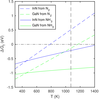
In OMVPE, a chemically active precursor such as ammonia is typically used to provide the high nitrogen activity required to grow group III nitrides. The need for this can be seen in Fig. 24, which shows the free energies of the reactions to form GaN and InN from the condensed metallic elements and either vapor N₂ or vapor NH₃ at 1 bar Chase (1998); Ambacher et al. (1996). At typical temperatures used for growth of high quality single crystal films at high rates (e.g. 1000 K for InN, 1300 K for GaN), the formation energy from N₂ is positive, indicating that the nitride is not stable and cannot be grown from N₂ at 1 bar. In contrast, the formation energies of the nitrides (plus H₂ at 1 bar) from the metals and NH₃ are negative at all relevant growth temperatures, indicating that growth from 1 bar of NH₃ is possible.

Figure 24: Free energy of formation as a function of temperature of InN and GaN from the liquid metals and either vapor N₂ or NH₃ at 1 bar Chase (1998); Ambacher et al. (1996). In the case of NH₃, this includes formation of H₂ at 1 bar.

However, actual OMVPE conditions do not correspond with equilibrium, because the very high partial pressures of N₂ and/or H₂ that would correspond to equilibrium with NH₃ at these temperatures are not allowed to accumulate. Thus, while formation of InN and GaN from NH₃ is energetically favored under OMVPE conditions, decomposition of these nitrides into N₂ is also energetically favored. This metastability is manifested in the oscillatory growth and decomposition of InN that has been observed Jiang et al. (2008). Thus the kinetics of the reaction steps that determine the nitrogen activity at the growth surface are critical to understanding and controlling OMPVE growth of metastable nitrides.

In previous work we have measured the trimethylindium (TMI) partial pressures required to condense InN and elemental In onto GaN (0001) Jiang et al. (2008). They can be analyzed to give experimentally determined values for the effective surface nitrogen activity arising from NH₃ under OMVPE conditions. The experiments were carried out using a very similar growth chamber Stephenson et al. (1999) as that used for the in-situ X-ray studies described below, using the same a total pressure of 0.267 bar, and the same NH₃ and carrier flows (2.7 standard liters per minute (slpm) NH₃ and 1.1 slpm N₂ in the group V channel, 0.9 slpm N₂ carrier gas for TMI in the group III channel). We have performed chamber flow modeling to calculate the equivalent TMI and NH₃ partial pressures $p_{TMI}$ and $p_{NH_{3}}$ above the center of the substrate surface as a function of inlet flows. At typical growth temperatures, an inlet flow of 0.184 $\mu$mol/min TMI corresponds to $p_{TMI}=1.22\times 10^{-6}$ bar, and an inlet flow of 2.7 slpm NH₃ corresponds to $p_{NH_{3}}=0.040$ bar.

Figure 25: Observed phase boundaries for condensation onto GaN (0001) of relaxed epitaxial InN (blue squares) and liquid elemental In (red circles) at $p_{NH_{3}}=0.040$ bar Jiang et al. (2008).

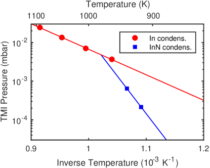
Figure 25 shows the $p_{TMI}$-$T$ boundaries determined by in-situ X-ray fluorescence and diffraction measurements for initial condensation of elemental In liquid or crystalline InN onto a GaN (0001) surface at $p_{NH_{3}}=0.040$ bar Jiang et al. (2008). At TMI partial pressures above the boundaries shown, the condensed phases nucleate and grow on the surface; at lower $p_{TMI}$, the condensed phases evaporate. The InN and In condensation boundaries intersect at 979 K.

A relationship between the nitrogen and indium activities at the InN condensation boundary can be obtained from the equilibrium

$${\rm In}_{vap}+\frac{1}{2}{\rm N}_{2}\leftrightarrow{\rm InN}_{sol},$$ (108)

which gives the chemical potential $\mu_{i}$ expression

$$\mu_{In}+\frac{1}{2}\mu_{N_{2}}=\mu_{InN},$$ (109)

and the activity $a_{i}$ expression

$$kT\log a_{In}+\frac{1}{2}kT\log a_{N_{2}}=\Delta G_{f}^{InN}(T),$$ (110)

where $\Delta G_{f}^{InN}(T)$ is the formation energy of InN from liquid In and N₂ at 1 bar shown in Figure 25. We assume that the activity of In relative to liquid In at the InN boundary is equal to the ratio $a_{In}=p_{TMI}^{InN}/p_{TMI}^{In}$, giving

$$kT\log a_{In}=kT\log p_{TMI}^{InN}-kT\log p_{TMI}^{In}$$ (111)

at the experimental condition, $p_{NH_{3}}=0.040$ bar. Equation (110) can then be used to obtain the nitrogen activity relative to 1 bar (i.e. effective partial pressure of N₂ in bar) for $p_{NH_{3}}=0.040$ bar.

Table 8: Evaluation of N₂ activity and $\Delta\mu_{Ga}$ at the GaN surface under OMVPE conditions. Formation energies of GaN and InN are from elements at standard conditions. TMI pressures at InN and In condensation boundaries are for $p_{NH_{3}}=0.04$ bar. Calculated $a_{N_{2}}$ and $\Delta\mu_{Ga}$ are thus also for $p_{NH_{3}}=0.04$ bar.

Quantity	Value as $f(T)$ (K)
	(eV)
$\Delta G_{f}^{GaN}$ Ambacher et al. (1996)	$-1.64+1.41\times 10^{-3}T$
$\Delta G_{f}^{InN}$ Ambacher et al. (1996)	$-1.39+1.78\times 10^{-3}T$
$kT\log p_{TMI}^{InN}$ Jiang et al. (2008)	$-1.309+0.88\times 10^{-3}T$
$kT\log p_{TMI}^{In}$ Jiang et al. (2008)	$-3.843+3.47\times 10^{-3}T$
$kT\log a_{In}$	$-2.534+2.59\times 10^{-3}T$
$=kT\log p_{TMI}^{InN}-kT\log p_{TMI}^{In}$
$kT\log a_{N_{2}}$	$2.288-1.63\times 10^{-3}T$
$=2(\Delta G_{f}^{InN}-kT\log a_{In})$
$\Delta\mu_{Ga}$	$-2.784+2.225\times 10^{-3}T$
$=\Delta G_{f}^{GaN}-0.5kT\log a_{N_{2}}$

Table 8 summarizes the calculations to obtain the nitrogen activity and $\Delta\mu_{Ga}$ under our OMVPE conditions. The value of $kT\log a_{N_{2}}=0.55$ eV at the experimental temperature $T=1073$ K gives the horizontal coordinate on the phase diagram from Eq. (107) as $\Delta\mu_{Ga}=-0.40$ eV. The value of $kT\log p_{NH_{3}}=-0.30$ eV at the experimental temperature $T=1073$ K gives the vertical coordinate on the phase diagram from Eq. (106) as $\Delta\mu_{NH_{3}}=-2.40$ eV. This position is shown on the predicted surface phase diagram, Fig. 15, with a rectangle representing the relatively large uncertainty in $\Delta\mu_{Ga}$.

A recent study of reconstructions on GaN (0001) in the OMVPE environment Kempisty and Kangawa (2019) included the effects of additional entropy associated with adsorbed species, which leads to a phase diagram that varies somewhat with temperature, even when expressed in chemical potential coordinates. These effects tend to stabilize reconstructions with H adsorbates at higher $T$, leading to a larger phase field for the 3H(T1) reconstruction than shown in Fig. 15. This is consistent with our finding that the 3H(T1) reconstruction agrees best with the experimental CTRs for all conditions studied.

Appendix B Atomic coordinates

Table 9: Fractional coordinates of bulk GaN used to calculate the substrate contribution to the CTRs.

Atom	Site	$x$	$y$	$z$
$k$	$n$
Ga	1	0.5000	0.1667	-0.5000
Ga	2	0.0000	0.6667	-0.5000
Ga	3	1.5000	0.1667	-0.5000
Ga	4	1.0000	0.6667	-0.5000
Ga	5	0.0000	0.0000	0.0000
Ga	6	0.5000	0.5000	0.0000
Ga	7	1.0000	0.0000	0.0000
Ga	8	1.5000	0.5000	0.0000
N	1	0.0000	0.0000	-0.6232
N	2	0.5000	0.5000	-0.6232
N	3	1.0000	0.0000	-0.6232
N	4	1.5000	0.5000	-0.6232
N	5	0.5000	0.1667	-0.1232
N	6	0.0000	0.6667	-0.1232
N	7	1.5000	0.1667	-0.1232
N	8	1.0000	0.6667	-0.1232

Table 10: Fractional coordinates $x$, $y$, $z$ of atoms in domain $j=1$ of the 3H(T1) reconstruction used to calculate the $\alpha$ terrace contribution to the CTRs, as well as their differences $\Delta x$, $\Delta y$, $\Delta z$ relative to bulk lattice positions. The differences for H atoms are relative to N sites. The lowest four Ga and N sites are an extra half unit cell of bulk lattice to account for the difference in height of the $\alpha$ and $\beta$ terraces.

Atom	Site	$x$	$y$	$z$	$\Delta x$	$\Delta y$	$\Delta z$
$k$	$n$
Ga	1	0.5000	0.1667	-0.5000	0.0000	0.0000	0.0000
Ga	2	0.0000	0.6667	-0.5000	0.0000	0.0000	0.0000
Ga	3	1.5000	0.1667	-0.5000	0.0000	0.0000	0.0000
Ga	4	1.0000	0.6667	-0.5000	0.0000	0.0000	0.0000
Ga	5	0.0000	0.0000	0.0076	0.0000	0.0000	0.0076
Ga	6	0.5075	0.4975	-0.0015	0.0075	-0.0025	-0.0015
Ga	7	1.0000	0.0050	-0.0015	0.0000	0.0050	-0.0015
Ga	8	1.4925	0.4975	-0.0015	-0.0075	-0.0025	-0.0015
Ga	9	0.4929	0.1643	0.5223	-0.0071	-0.0024	0.0223
Ga	10	0.0000	0.6667	0.4294	0.0000	0.0000	-0.0706
Ga	11	1.5071	0.1643	0.5223	0.0071	-0.0024	0.0223
Ga	12	1.0000	0.6714	0.5223	0.0000	0.0047	0.0223
N	1	0.0000	0.0000	-0.6232	0.0000	0.0000	0.0000
N	2	0.5000	0.5000	-0.6232	0.0000	0.0000	0.0000
N	3	1.0000	0.0000	-0.6232	0.0000	0.0000	0.0000
N	4	1.5000	0.5000	-0.6232	0.0000	0.0000	0.0000
N	5	0.4988	0.1663	-0.1254	-0.0012	-0.0004	-0.0022
N	6	0.0000	0.6667	-0.1201	0.0000	0.0000	0.0031
N	7	1.5012	0.1663	-0.1254	0.0012	-0.0004	-0.0022
N	8	1.0000	0.6675	-0.1254	0.0000	0.0008	-0.0022
N	9	0.0000	0.0000	0.3766	0.0000	0.0000	-0.0002
N	10	0.5064	0.4979	0.3775	0.0064	-0.0021	0.0007
N	11	1.0000	0.0043	0.3775	0.0000	0.0043	0.0007
N	12	1.4936	0.4979	0.3775	-0.0064	-0.0021	0.0007
H	13	0.5002	0.1667	0.8196	0.0002	0.0000	-0.0572
H	15	1.4998	0.1667	0.8196	-0.0002	0.0001	-0.0572
H	16	1.0000	0.6666	0.8196	0.0000	-0.0001	-0.0572

Table 11: Fractional coordinates $x$, $y$, $z$ of atoms in domain $j=1$ of the 3H(T1) reconstruction used to calculate the $\beta$ terrace contribution to the CTRs, as well as their differences $\Delta x$, $\Delta y$, $\Delta z$ relative to bulk lattice positions. The differences for H atoms are relative to N sites.

Atom	Site	$x$	$y$	$z$	$\Delta x$	$\Delta y$	$\Delta z$
$k$	$n$
Ga	1	0.5075	0.1692	-0.5015	0.0075	0.0025	-0.0015
Ga	2	0.0000	0.6667	-0.4924	0.0000	0.0000	0.0076
Ga	3	1.4925	0.1692	-0.5015	-0.0075	0.0025	-0.0015
Ga	4	1.0000	0.6617	-0.5015	0.0000	-0.0050	-0.0015
Ga	5	0.0000	0.0000	-0.0706	0.0000	0.0000	-0.0706
Ga	6	0.4929	0.5024	0.0223	-0.0071	0.0024	0.0223
Ga	7	1.0000	-0.0047	0.0223	0.0000	-0.0047	0.0223
Ga	8	1.5071	0.5024	0.0223	0.0071	0.0024	0.0223
N	1	0.0000	0.0000	-0.6201	0.0000	0.0000	0.0031
N	2	0.4988	0.5004	-0.6254	-0.0012	0.0004	-0.0022
N	3	1.0000	-0.0008	-0.6254	0.0000	-0.0008	-0.0022
N	4	1.5012	0.5004	-0.6254	0.0012	0.0004	-0.0022
N	5	0.5064	0.1688	-0.1225	0.0064	0.0021	0.0007
N	6	0.0000	0.6667	-0.1234	0.0000	0.0000	-0.0002
N	7	1.4936	0.1688	-0.1225	-0.0064	0.0021	0.0007
N	8	1.0000	0.6624	-0.1225	0.0000	-0.0043	0.0007
H	10	0.5002	0.5000	0.3196	0.0002	-0.0000	-0.0572
H	11	1.0000	0.0001	0.3196	0.0000	0.0001	-0.0572
H	12	1.4998	0.4999	0.3196	-0.0002	-0.0001	-0.0572

To provide a detailed example of how we calculate the CTR intensities including the effects of reconstruction, we here provide an example of the atomic coordinates for a particular reconstruction. The qualitative behavior we observe, that $f_{\alpha}^{ss}$ increases with growth rate, does not depend upon the reconstruction chosen or the exact values of the atomic coordinates used. These affect only the precise values of $f_{\alpha}^{ss}$ obtained, as shown in Table 1.

Tables 9, 10, and 11 give the atomic coordinates for the 3H(T1) reconstruction obtained in Walkosz et al. (2012). The fractional coordinates $x$, $y$, and $z$ given in the tables are the components of the positions $\mathbf{r}_{kn}$, $\mathbf{r}_{jkn}^{\alpha}$, and $\mathbf{r}_{jkn}^{\beta}$ used to calculate the structure factors, normalized to the respective orthohexagonal lattice parameters $a$, $b$, and $c$, i.e. $\mathbf{r}=(ax,by,cz)$. A $2\times 2$ surface unit cell is used, equivalent to two orthohexagonal unit cells, so there are 8 Ga and 8 N sites in each. These coordinates place a bulk Ga site on a $\beta$ layer at the origin. We use $u=0.3768$ for the internal lattice parameter of bulk GaN, i.e. the fractional distance between Ga and N sites, which deviates slightly from the ideal $3/8$ value as found in ab initio calculations Walkosz et al. (2012); Stampfl and Van de Walle (1999) and experiments Minikayev et al. (2015). Relaxed positions were calculated for a one-unit-cell thick layer at the surface. For the $\alpha$ terrace, and extra half unit cell of bulk (unrelaxed) atoms is attached to the bottom to account for the difference in height of the $\alpha$ and $\beta$ terraces, as shown in Fig. 6. Coordinates for only one domain are given. Those for other 5 domains are obtained by 3-fold rotation about the $6_{3}$ axis and/or reflection of the $y$ coordinate. One can see that the Ga atoms bonded to the three adsorbed hydrogens of the 3H(T1) reconstruction relax to higher $z$ positions.

Appendix C Deposition and evaporation rates

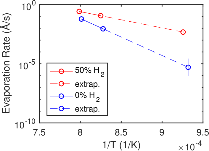
Under the OMVPE conditions used, we observe that deposition of GaN is Ga transport limited (i.e. the deposition rate is proportional to the TEGa supply rate, nearly independent of $T$ and NH₃ supply), and the net growth rate has a negative offset at zero TEGa supply corresponding to an evaporation rate that depends on $T$ and the carrier gas composition (e.g. presence or absence of H₂). To determine the deposition rate for the conditions used in the X-ray study, we used the deposition efficiency (deposition rate per TEGa supply rate) determined from previous studies of CTR oscillations during layer-by-layer growth Perret et al. (2014); Ju et al. (2019). We also measured the evaporation rates at two higher temperatures and both carrier gas compositions (0% and 50% H₂), and extrapolated them to the lower temperatures studied here.

Figure 26: Growth rate as a function of TEGa supply determined from CTR oscillations during layer-by-layer growth. Line is fit to new chamber data giving a deposition efficiency of 1.0 (Å/s)/($\mu$mole/min).

Figure 27: Reflected laser signal during growth under various conditions. Vertical dashed lines show times at which conditions changed.

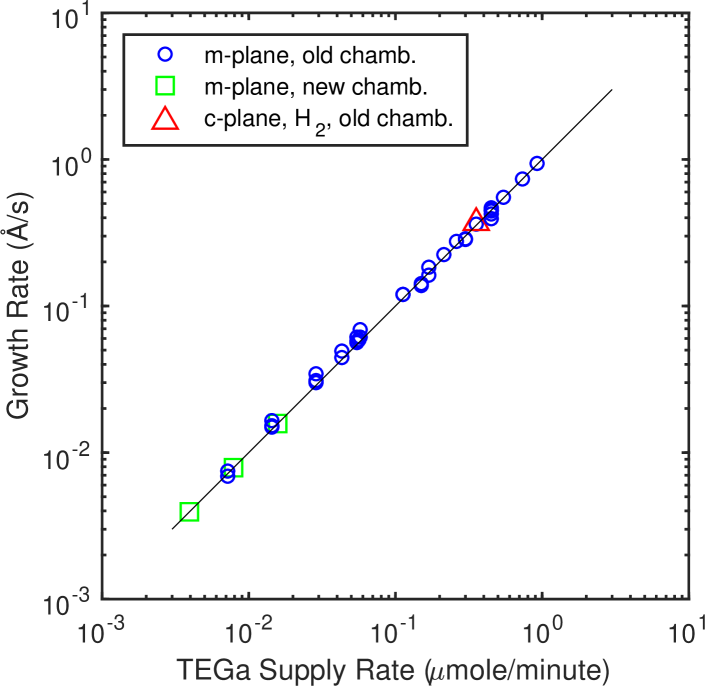
Figure 26 shows the growth rates measured from CTR oscillations during layer-by-layer growth as a function of TEGa supply Perret et al. (2014); Ju et al. (2019). In all cases the chamber flows were the same as in the X-ray study reported here (e.g. 2.7 slpm NH₃, 267 mbar total pressure). Almost all data points are for growth on m-plane $(10\overline{1}0)$ GaN in N₂ carrier gas (0% H₂), which exhibits layer-by-layer mode over a wide range of conditions. Data are shown from both a previous growth chamber (“old” chamber) Stephenson et al. (1999) and the current growth chamber (“new” chamber) Ju et al. (2017, 2019). The chambers were designed to have the same flow geometry, and the growth behavior of both appear to be identical. The data points from the previous chamber range in temperature from $848$ K to $1064$ K; the data points for the current chamber are for $867$ K. The line shown is a fit to the data from the current chamber, which gives a deposition efficiency of 1.0 (Å/s)/($\mu$mole/min). One data point is shown for growth on c-plane (0001) GaN in 50% N₂ + 50% H₂ carrier gas at $900$ K; layer-by-layer growth was only observed on (0001) GaN under this condition. It agrees with the m-plane data obtained in 0% H₂ carrier, suggesting that the same deposition efficiency can be used for (0001) GaN in either 0% or 50% H₂ carrier gas. We expect that there is negligible evaporation at $900$ K in either carrier gas.

Figure 28: Added thickness during growth under various conditions. Vertical dashed lines show times at which conditions changed.

Figure 29: Added thickness during growth under TEGa flows shown ($\mu$mol/min) at T = 1252K, 50% H₂. Vertical dashed lines show times at which conditions changed. Black lines show fits to extract net growth rates.

Figure 30: Evaporation rate at zero TEGa flow as a function of $T$, with and without H₂, with extrapolation to lower $T$.

Table 12: Values of net growth rate $Gc/2$ extracted from laser interferometry measurements for two temperatures and for carrier gas with and without H₂, as a function of TEGa flow $f_{TEGa}$. Also shown is fitted $d(Gc/2)/df_{TEGa}$ for each $T$ and carrier gas.

$T$	H2	$f_{TEGa}$	$Gc/2$	$d(Gc/2)/df_{TEGa}$
(K)	in	($\mu$mol	(Å/s)	(Å/s)/
	carr.	/min)		($\mu$mol/min)
1208	0%	0.00	$-0.009\pm 0.003$	$1.19\pm 0.03$
		0.09	$0.092\pm 0.003$
		0.33	$0.322\pm 0.004$
		1.34	$1.582\pm 0.002$
1212	50%	0.00	$-0.115\pm 0.002$	$1.38\pm 0.05$
		0.09	$-0.038\pm 0.002$
		0.33	$0.248\pm 0.003$
		1.34	$1.705\pm 0.002$
1248	0%	0.00	$-0.061\pm 0.004$	$1.27\pm 0.05$
		0.16	$0.042\pm 0.004$
		0.33	$0.268\pm 0.005$
		1.34	$1.584\pm 0.002$
1252	50%	0.00	$-0.265\pm 0.004$	$1.40\pm 0.03$
		0.16	$-0.050\pm 0.003$
		0.33	$0.134\pm 0.001$
		1.34	$1.562\pm 0.001$

To determine the evaporation rate at the temperature used in the X-ray study presented here (e.g. $1080$ K), we used laser interferometry to observe the change in thickness of an (0001) GaN film on a sapphire substrate Ju et al. (2017); Koleske et al. (2005), under conditions of both growth and evaporation at higher $T$. As the film thickness $d(t)$ changes during growth or evaporation, the back-scattered laser intensity $I(t)$ oscillates with time $t$ due to interference between light reflected from the film surface and the substrate/film interface, according to

$$I(t)-I_{min}=[I_{max}-I_{min}]\left(\frac{1+\cos[2\pi d(t)/d_{0}]}{2}\right),$$ (112)

where $I_{min}(t)$ and $I_{max}(t)$ are the envelope of the minima and maxima, which can vary with time as film roughness changes, and the thickness oscillation period is $d_{0}=\lambda/2n$, where $\lambda=6330$ Å is the wavelength of the light and $n$ is the refractive index of GaN. This can be inverted to obtain the thickness evolution as

$$d(t)=\left(\frac{d_{0}}{2\pi}\right)\cos^{-1}\left(\frac{2[I(t)-I_{min}(t)]}{I_{max}(t)-I_{min}(t)}-1\right).$$ (113)

Figure 27 shows the evolution of the laser signal with time during the experiment. We began by growing a full oscillation at a high growth rate to obtain initial values for $I_{min}$ and $I_{max}$. Once the signal had reach a value intermediate between these limits, where the phase of the oscillation is most accurately determined, we changed the TEGa flow $f_{TEGa}$ to observe the net growth or evaporation rate at some fixed values of $f_{TEGa}$. Then we changed $T$ and/or the carrier gas concentration, and repeated the process starting with growing a full oscillation at a high rate. The blue dashed curves in Fig. 27 show the interpolated $I_{min}(t)$ and $I_{max}(t)$ envelopes. Figure 28 shows the thickness change with time extracted with Eq. (113), using a value of $d_{0}=1302$ Å corresponding to $n=2.431$ Tapping and Reilly (1986); Touloulian et al. (1977). Figure 29 shows an expanded region of the thickness evolution, where we varied $f_{TEGa}$ at $T=1252$ K and 50% H₂ fraction. The solid lines show linear fits to extract the net growth rate in Å/s, $Gc/2$, at each value of $f_{TEGa}$. Similar fits were done for the regions at different $T$ and H₂ fraction, and the extracted growth rates are given in Table 12.

We observe that $Gc/2$ becomes negative at $f_{TEGa}=0$ due to evaporation, and that evaporation is more rapid at higher $T$ and when H₂ is present in the carrier gas. These evaporation rates in 50% H₂ are similar to the rate of $4.2\times 10^{18}$ m^-2s^-1 $=0.37$ ML/s obtained by Koleske et al. (2001) at 1300 K with H₂ and NH₃ at a total pressure of $267$ mbar. Also shown in Table 12 is the deposition efficiency $d(Gc/2)/df_{TEGa}$ obtained from a fit to $Gc/2$ at the four values of $f_{TEGa}$ for each $T$ and H₂ fraction. The values are all similar to but slightly higher than the value of $d(Gc/2)/df_{TEGa}=1.0$ (Å/s)/($\mu$mole/min) that we have observed from growth oscillations during layer-by-layer growth at lower $T$, described above Ju et al. (2019); Perret et al. (2014). The efficiency seems to be slightly larger for 50% H₂ compared with 0% H₂. This may indicate that the deposition efficiency can vary somewhat as the flow and diffusion fields vary in the chamber with $T$ or carrier gas composition.

To obtain the evaporation rate at $f_{TEGa}=0$ at the lower $T$ used in the x-ray experiments reported above, we extrapolated the values for 50% H₂ or 0% H₂ assuming Arrhenius behavior of the evaporation rate, as shown in Fig. 30. The fitted activation energies are $2.7\pm 0.1$ and $6.2\pm 1.2$ eV in 50% and 0% H₂, respectively. We obtain evaporation rates of $4.8\pm 0.8\times 10^{-3}$ Å/s at $T=1080$K with 50% H₂, and $5\times 10^{-6}$ Å/s (with error limits of a factor of 5) at $T=1073$K with 0% H₂. We have used these evaporation rates, as well as the low-temperature deposition efficiency of $1.0$ (Å/s)/($\mu$mole/min) and the TEGa flow rates of $0$ or $0.033$ $\mu$mole/min, to calculate the net growth rates in Table 1.

References

- Burton et al. (1951) W. Burton, N. Cabrera, and F. Frank, “The growth of crystals and the equilibrium structure of their surfaces,” Philos. Trans. Royal. Soc. London Ser. A 243, 299 (1951).
- Jeong and Williams (1999) Hyeong-Chai Jeong and Ellen D. Williams, “Steps on surfaces: experiment and theory,” Surf. Sci. Rep. 34, 171–294 (1999).
- Woodruff (2015) D. P. Woodruff, “How does your crystal grow? a commentary on Burton, Cabrera and Frank (1951) ‘The growth of crystals and the equilibrium structure of their surfaces’,” Phil. Trans. R. Soc. A. 373, 20140230 (2015).
- Tsao (1993) Jeffrey Y. Tsao, Materials Fundamentals of Molecular Beam Epitaxy (Academic Press, Inc., San Diego, CA, 1993) pp. 201–257.
- van Enckevort and Bennema (2004) W. J. P. van Enckevort and P. Bennema, “Interlacing of growth steps on crystal surfaces as a consequence of crystallographic symmetry,” Acta Crystallogr. Sec. A 60, 532–541 (2004).
- Tromp et al. (1985) R. M. Tromp, R. J. Hamers, and J. E. Demuth, “Si (001) dimer structure observed with scanning tunneling microscopy,” Phys. Rev. Lett. 55, 1303 (1985).
- Xie et al. (1999) M. H. Xie, S. M. Seutter, W. K. Zhu, L. X. Zheng, Huasheng Wu, and S. Y. Tong, “Anisotropic step-flow growth and island growth of GaN(0001) by molecular beam epitaxy,” Phys. Rev. Lett. 82, 2749–2752 (1999).
- Giesen (2001) Margret Giesen, “Step and island dynamics at solid/vacuum and solid/liquid interfaces,” Prog. Surf. Sci. 68, 1–154 (2001).
- Verma (1951) Ajit Ram Verma, “CI. Observations on carborundum of growth spirals originating from screw dislocations,” Philos. Mag. 42, 1005–1013 (1951).
- Sunagawa and Bennema (1979) I. Sunagawa and P. Bennema, “Modes of vibrations in step trains: Rhythmical bunching,” J. Cryst. Growth 46, 451–457 (1979).
- van der Hoek et al. (1982) B. van der Hoek, J. P. van der Eerden, and K. Tsukamoto, “Interpretation of double spirals on silicon carbide,” J. Cryst. Growth 58, 545–553 (1982).
- Heying et al. (1999) B. Heying, E. J. Tarsa, C. R. Elsass, P. Fini, S. P. DenBaars, and J. S. Speck, “Dislocation mediated surface morphology of GaN,” J. Appl. Phys. 85, 6470–6476 (1999).
- S Vézian et al. (2001) S. S Vézian, J. Massies, F. Semond, and N. Grandjean, “Surface morphology of GaN grown by molecular beam epitaxy,” Mater. Sci. Eng. B 82, 56–58 (2001).
- Zauner et al. (2002) A. R. A Zauner, E. Aret, W. J. P. van Enckevort, J. L. Weyher, S. Porowski, and J. J. Schermer, “Homo-epitaxial growth on the N-face of GaN single crystals: the influence of the misorientation on the surface morphology,” J. Cryst. Growth 240, 14–21 (2002).
- Xie et al. (2006) M. H. Xie, M. Gong, E. K. Y. Pang, H. S. Wu, and S. Y. Tong, “Origin of triangular island shape and double-step bunching during GaN growth by molecular-beam epitaxy under excess Ga conditions,” Phys. Rev. B 74, 085314 (2006).
- Krukowski et al. (2007) S. Krukowski, P. Kempisty, P. Str ak, G. Nowak, R. Czernecki, M. Leszczynski, T. Suski, M. Bockowski, and I. Grzegory, “Modelling the growth of nitrides in ammonia-rich environment,” Cryst. Res. Technol. 42, 1281–1290 (2007).
- Zheng et al. (2008) Hao Zheng, M. H. Xie, H. S. Wu, and Q. K. Xue, “Kinetic energy barriers on the GaN(0001) surface: A nucleation study by scanning tunneling microscopy,” Phys. Rev. B 77, 045303 (2008).
- Turski et al. (2013) H. Turski, M. Siekacz, Z. R. Wasilewski, M. Sawicka, S. Porowski, and C. Skierbiszewski, “Nonequivalent atomic step edges - role of gallium and nitrogen atoms in the growth of InGaN layers,” J. Cryst. Growth 367, 115–121 (2013).
- Lin et al. (2013) Chia-Hung Lin, Tetsuya Akasaka, and Hideki Yamamoto, “Nucleus and spiral growth of N-face GaN(000) obtained by selective-area metalorganic vapor phase epitaxy,” Appl. Phys Express 6, 035503 (2013).
- Pristovsek et al. (2017) Markus Pristovsek, Konrad Bellman, Frank Mehnke, Joachim Stellmach, Tim Wernicke, and Michael Kneissl, “Surface reconstructions of (0001) AlN during metal-organic vapor phase epitaxy,” Phys. Status Solidi B 254, 1600711 (2017).
- Chen et al. (2002) Yefan Chen, Hang-Ju Ko, Soon-Ku Hong, Takafumi Yao, and Yusaburo Segawa, “Morphology evolution of ZnO(000) surface during plasma-assisted molecular-beam epitaxy,” Appl. Phys. Lett. 80, 1358–1360 (2002).
- Załuska-Kotur et al. (2011) Magdalena A. Załuska-Kotur, Filip Krzyżewski, and Stanisław Krukowski, “Double step structure and meandering due to the many body interaction at GaN(0001) surface in N-rich conditions,” J. Appl. Phys. 109, 023515 (2011).
- Załuska-Kotur et al. (2010) Magdalena A. Załuska-Kotur, Filip Krzyżewski, and Stanisław Krukowski, “Surface patterns due to step flow anisotropy formed in crystal growth process,” J. Non-Cryst. Solids 356, 1935–1939 (2010).
- Xu et al. (2017) Dongwei Xu, Peter Zapol, G. Brian Stephenson, and Carol Thompson, “Kinetic monte carlo simulations of GaN homoepitaxy on c- and m-plane surfaces,” J. Chem. Phys. 146, 144702 (2017).
- Chugh and Ranganathan (2017a) Manjusha Chugh and Madhav Ranganathan, “Lattice kinetic monte carlo simulation study of the early stages of epitaxial GaN(0001) growth,” Appl. Surf. Sci. 422, 1120–1128 (2017a).
- Akiyama et al. (2020a) Toru Akiyama, Takumi Ohka, Kohji Nakamura, and Tomonori Ito, “Ab initio study for adsorption and desorption behavior at step edges of GaN(0001) surface,” J. Cryst. Growth 532, 125410 (2020a).
- Akiyama et al. (2020b) Toru Akiyama, Takumi Ohka, Kohji Nakamura, and Tomonori Ito, “Ab initio study for adsorption and desorption behavior at step edges of AlN(0001) and GaN(0001) surfaces,” Jpn. J. Appl. Phys. 59, SGGK03 (2020b).
- Avery et al. (1997) A. R. Avery, H. T. Dobbs, D. M. Holmes, B. A. Joyce, and D. D. Vvedensky, “Nucleation and growth of islands on GaAs surfaces,” Phys. Rev. Lett. 79, 3938–3941 (1997).
- Jo et al. (2012) Masafumi Jo, Takaaki Mano, Marco Abbarchi, Takashi Kuroda, Yoshiki Sakuma, and Kasuaki Sakoda, “Self-limiting growth of hexagonal and triangular quantum dots on (111)A,” Cryst. Growth Des. 12, 1411–1415 (2012).
- Kalff et al. (1998) Matthias Kalff, George Comsa, and Thomas Michely, “How sensitive is epitaxial growth to adsorbates?” Phys. Rev. Lett. 81, 1255–1258 (1998).
- Yin et al. (2009) Cong Yin, Xi-Jing Ning, Jun Zhuang, Yi-Qun Xie, Xiu-Fang Gong, Xiang-Xi Ye, Chen Ming, and Yun-Fei Jin, “Shape prediction of two-dimensional adatom islands on crystal surfaces during homoepitaxial growth,” Appl. Phys. Lett. 94, 183107 (2009).
- Robinson (1986) Ian K. Robinson, “Crystal truncation rods and surface roughness,” Phys. Rev. B 33, 3830 (1986).
- Walkosz et al. (2012) Weronika Walkosz, Peter Zapol, and G. Brian Stephenson, “Metallicity of InN and GaN surfaces exposed to NH3,” Phys. Rev. B 85, 033308 (2012).
- Otte and Crocker (1965) H. M. Otte and A. G. Crocker, “Crystallographic formulae for hexagonal lattices,” Phys. Status Solidi 9, 441–450 (1965).
- Munkholm and Brennan (1999) A. Munkholm and S. Brennan, “Influence of miscut on crystal truncation rod scattering,” J. Appl. Crystallogr. 32, 143–153 (1999).
- Trainor et al. (2002) Thomas P. Trainor, Peter J. Eng, and Ian K. Robinson, “Calculation of crystal truncation rod structure factors for arbitrary rational surface terminations,” J. Appl. Crystallogr. 35, 696–701 (2002).
- Waasmaier and Kirfel (1995) D. Waasmaier and A. Kirfel, “New analytical scattering-factor functions for free atoms and ions,” Acta Crystallogr. Sec. A 51, 416–431 (1995).
- Henke et al. (1993) B. L. Henke, E. M. Gullikson, and J. C. Davis, “X-ray interactions: photoabsorption, scattering, transmission, and reflection at E=50-30000 eV, Z=1-92,” At. Data Nucl. Data Tables 54, 181 (1993), updates at https://henke.lbl.gov/optical_constants/asf.html.
- Ju et al. (2017) Guangxu Ju, Matthew J. Highland, Angel Yanguas-Gil, Carol Thompson, Jeffrey A. Eastman, Hua Zhou, Sean M. Brennan, G. Brian Stephenson, and Paul H. Fuoss, “An instrument for in situ coherent x-ray studies of metal-organic vapor phase epitaxy of III-nitrides,” Rev. Sci. Instrum. 88, 035113 (2017).
- Ju et al. (2018) Guangxu Ju, Matthew J. Highland, Carol Thompson, Jeffrey A. Eastman, Paul H. Fuoss, Hua Zhou, Roger Dejus, and G. Brian Stephenson, “Characterization of the x-ray coherence properties of an undulator beamline at the Advanced Photon Source,” J. of Synchrotron Radiat. 25, 1036–1047 (2018).
- Ju et al. (2019) Guangxu Ju, Dongwei Xu, Matthew J. Highland, Carol Thompson, Hua Zhou, Jeffrey A. Eastman, Paul H. Fuoss, Peter Zapol, Hyunjung Kim, and G. Brian Stephenson, “Coherent x-ray spectroscopy reveals the persistence of island arrangements during layer-by-layer growth,” Nat. Phys. 15, 589–594 (2019).
- Note (1) GANKIBANTM from SixPoint Materials, Inc., spmaterials.com.
- Murty et al. (2000) M. V. Ramana Murty, P. Fini, G. B. Stephenson, Carol Thompson, J. A. Eastman, A. Munkholm, O. Auciello, R. Jothilingam, S. P. DenBaars, and J. S. Speck, “Step bunching on the vicinal GaN (0001) surface,” Phys. Rev. B 62, R10661 (2000).
- Kempisty and Kangawa (2019) Pawel Kempisty and Yoshihiro Kangawa, “Evolution of the free energy of the GaN (0001) surface based on first-principles phonon calculations,” Phys. Rev. B 100, 085304 (2019).
- Guin et al. (2020) L. Guin, M. E. Jabbour, L. Shaabani-Ardali, L. Benoit-Maréchal, and N. Triantafyllidis, “Stability of vicinal surfaces: Beyond the quasistatic approximation,” Phys. Rev. Lett. 124, 036101 (2020).
- Li et al. (2016) Yuan Li, Xuejiang Chen, and Juan Su, “Study on formation of step bunching on 6H-SiC (0001) surface by kinetic Monte Carlo method,” Appl. Surf. Sci. 371, 242–247 (2016).
- Bellmann et al. (2017) Konrad Bellmann, Udo W. Pohl, Christian Kuhn, Tim Wernicke, and Michael Kneissl, “Controlling the morphology transition between step-flow growth and step-bunching growth,” J. Cryst. Growth 478, 187–192 (2017).
- Dufay et al. (2007) Matthieu Dufay, Thomas Frisch, and Jean-Marc Debierre, “Role of step-flow advection during electromigration-induced step bunching,” Phys. Rev. B 75, 241304 (2007).
- Pierre-Louis (2003a) O. Pierre-Louis, “Step bunching with general step kinetics: stability analysis and macroscopic models,” Surf. Sci. 529, 114–134 (2003a).
- Pimpinelli and Videcoq (2000) A. Pimpinelli and A. Videcoq, “Novel mechanism for the onset of morphological instabilities during chemical vapour epitaxial growth,” Surf. Sci. 445, L23–L28 (2000).
- Pierre-Louis and Métois (2004) O. Pierre-Louis and J.-J. Métois, “Kinetic step pairing,” Phys. Rev. Lett. 93, 165901 (2004).
- Patrone et al. (2010) Paul N. Patrone, T. L. Einstein, and Dionisios Margetis, “One-dimensional model of interacting-step fluctuations on vicinal surfaces: Analytical formulas and kinetic Monte Carlo simulations,” Phys. Rev. E 82, 061601 (2010).
- Ranguelov et al. (2007) Bogdan Ranguelov, M. S. Altman, and Ivan Markov, “Critical terrace width for step flow growth: Effect of attachment-detachment asymmetry and step permeability,” Phys. Rev. B 75, 245419 (2007).
- Hanada (2019) Takashi Hanada, “Thermodynamic model for metalorganic vapor-phase epitaxy of N-polar group-III nitrides in step-flow growth mode: Hydrogen, competitive adsorption, and configuration entropy,” Phys. Rev. Materials 3, 103404 (2019).
- Pierre-Louis (2003b) O. Pierre-Louis, “Phase field models for step flow,” Phys. Rev. E 68, 021604 (2003b).
- Reeber and Wang (2000) Robert R. Reeber and Kai Wang, “Lattice parameters and thermal expansion of GaN,” J. Mater. Res. 15, 40–44 (2000).
- Zywietz et al. (1998) Tosja Zywietz, Jörg Neugebauer, and Matthias Scheffler, “Adatom diffusion at GaN(0001 and (000) surfaces,” Appl. Phys. Lett. 73, 487–489 (1998).
- Chugh and Ranganathan (2017b) Manjusha Chugh and Madhav Ranganathan, “Adsorbate interactions on the GaN(0001) surface and their effect on diffusion barriers and growth morphology,” Phys. Chem. Chem. Phys. 19, 2111–2123 (2017b).
- González-Hernández et al. (2011) Rafael González-Hernández, William López-Pérez, María Guadalupe Moreno-Armenta, and Jairo Arbey Rodríguez M, “Adsorption and diffusion of 3d transition metal atoms on the GaN(0001) surface,” J. Appl. Phys. 110, 083712 (2011).
- Koleske et al. (2014) D. D. Koleske, S. R. Lee, M. H. Crawford, K. C. Cross, M. E. Coltrin, and J. M. Kempisty, “Connection between GaN and InGaN growth mechanisms and surface morphology,” J. Cryst. Growth 391, 85–96 (2014).
- Shewmon (1989) Paul Shewmon, Diffusion in Solids, 2nd ed. (Springer, 1989).
- Van de Walle and Neugebauer (2002a) Chris G. Van de Walle and J. Neugebauer, “First-principles surface phase diagram for hydrogen on GaN surfaces,” Phys. Rev. Lett. 88, 066103 (2002a).
- Van de Walle and Neugebauer (2002b) Chris G. Van de Walle and J. Neugebauer, “Role of hydrogen in surface reconstructions and growth of GaN,” J. Vac. Sci. Technol. B 20, 1640–1646 (2002b).
- Chase (1998) Malcolm W. Chase, Jr., “NIST-JANAF thermochemical tables (4th edition),” J. Phys. Chem. Ref. Data, Monograph 9 , 1–1151 (1998).
- Ambacher et al. (1996) O. Ambacher, M. S. Brandt, R. Dimitrov, T. Metzger, M. Stutzmann, R. A. Fischer, A. Miehr, A. Bergmaier, and G. Dollinger, “Thermal stability and desorption of Group III nitrides prepared by metal organic chemical vapor deposition,” J. Vac. Sci. Technol. B 14, 3532–3542 (1996).
- Jiang et al. (2008) Fan Jiang, A. Munkholm, R.-V. Wang, S. K. Streiffer, Carol Thompson, P. H. Fuoss, K. Latifi, K. R. Elder, and G. B. Stephenson, “Spontaneous oscillations and waves during chemical vapor deposition of InN,” Phys. Rev. Lett. 101, 086102 (2008), (See online supplemental for trimethylindium (TMI) partial pressures required to condense InN and elemental In).
- Stephenson et al. (1999) G. B. Stephenson, J. A. Eastman, O. Auciello, A. Munkholm, Carol Thompson, P. H. Fuoss, P. Fini, S. P. DenBaars, and J. S. Speck, “Real-time x-ray scattering studies of surface structure during metalorganic chemical vapor deposition of GaN,” MRS Bull. 24[1], 21 (1999).
- Stampfl and Van de Walle (1999) C. Stampfl and C. G. Van de Walle, “Density-functional calculations for III-V nitrides using the local-density approximation and the generalized gradient approximation,” Phys. Rev. B 59, 5521–5535 (1999).
- Minikayev et al. (2015) R. Minikayev, W. Paszkowicz, P. Piszora, M. Knapp, C. Bähtz, and S. Podsiadło, “Thermal expansion of polycrystalline gallium nitride: an x-ray diffraction study,” X-Ray Spectrom. 44, 382–388 (2015).
- Perret et al. (2014) Edith Perret, M. J. Highland, G. B. Stephenson, S. K. Streiffer, P. Zapol, P. H. Fuoss, A. Munkholm, and Carol Thompson, “Real-time x-ray studies of crystal growth modes during metal-organic vapor phase epitaxy of GaN on c- and m-plane single crystals,” Appl. Phys. Lett. 105, 051602 (2014).
- Koleske et al. (2005) D. D. Koleske, M. E. Coltrin, and M. J. Russell, “Using optical reflectance to measure GaN nucleation layer decomposition layer kinetics,” J. Cryst. Growth 279, 37–54 (2005).
- Tapping and Reilly (1986) J. Tapping and M. L. Reilly, “Index of refraction of sapphire between 24 and 1060 C for wavelengths of 633 and 799 nm,” J. Opt. Soc. Am. A 3, 610–616 (1986).
- Touloulian et al. (1977) Y. S. Touloulian, R. K. Kirby, R. E. Taylor, and T. Y. Lee, Thermal Expansion: Nonmetallic Solids, Vol. 13 (Springer, 1977) pp. 154–389.
- Koleske et al. (2001) D. D. Koleske, A. E. Wickenden, R. L. Henry, Culbertson. J. C., and M. E. Twigg, “GaN decomposition in H2 and N2 at MOVPE temperatures and pressures,” J. Cryst. Growth 223, 466–483 (2001).