A Kernel-Based Approach to Non-Stationary
Reinforcement Learning in Metric Spaces
Omar D. Domingues1,2 Pierre Ménard3 Matteo Pirotta4 Emilie Kaufmann1,2,5 Michal Valko1,6 1Inria Lille 2Université de Lille 3OvGU 4Facebook AI Research 5CNRS 6DeepMind Paris
Abstract
In this work, we propose KeRNS: an algorithm for episodic reinforcement learning in non-stationary Markov Decision Processes (MDPs) whose state-action set is endowed with a metric. Using a non-parametric model of the MDP built with time-dependent kernels, we prove a regret bound that scales with the covering dimension of the state-action space and the total variation of the MDP with time, which quantifies its level of non-stationarity. Our method generalizes previous approaches based on sliding windows and exponential discounting used to handle changing environments. We further propose a practical implementation of KeRNS, we analyze its regret and validate it experimentally.
1 Introduction
In reinforcement learning (RL), an agent interacts with an environment by sequentially taking actions, receiving rewards and observing state transitions. One of the main challenges in RL is the trade-off between exploration, the act of gathering information about the environment, and exploitation, the act of using the current knowledge to maximize the sum of rewards. In non-stationary environments, handling this trade-off becomes much harder: what has been learned in the past may no longer be valid in the present. Therefore, the agent needs to constantly re-explore previously known parts of the environment to discover possible changes. In this work, we propose KeRNS,111meaning Kernel-based Reinforcement Learning in Non-Stationary environments. an algorithm that handles this problem by acting optimistically and by forgetting data that are far in the past, which naturally causes the agent to keep exploring to discover changes. KeRNS relies on non-parametric kernel estimators of the MDP, and the non-stationarity is handled by using time-dependent kernels.
The regret of an algorithm, defined as the difference between the rewards obtained by an optimal agent and the ones obtained by the algorithm, allows us to quantify how well an agent balances exploration and exploitation. We prove a regret bound for KeRNS that holds in a challenging setting, where the state-action space can be continuous and the environment can change in every episode, as long as the cumulative changes remain small when compared to the total number of episodes.
Related work Regret bounds for RL in stationary environments have been extensively studied in finite (tabular) MDPs (Jaksch et al.,, 2010; Azar et al.,, 2017; Dann et al.,, 2017; Jin et al.,, 2018; Zanette and Brunskill,, 2019), and also in metric spaces under Lipschitz continuity assumptions (Ortner and Ryabko,, 2012; Song and Sun,, 2019; Sinclair et al.,, 2019; Domingues et al.,, 2020; Sinclair et al.,, 2020). Recent works provide algorithms with regret bounds for non-stationary RL in the tabular setting (Gajane et al.,, 2018; Ortner et al.,, 2019; Cheung et al.,, 2020). These algorithms estimate the transitions and the rewards in an episode using the data observed up to episode . However, since the MDP can change from one episode to another, these estimators are biased. If nothing is done to handle this bias, the algorithms will suffer a linear regret (Ortner et al.,, 2019) that depends on the magnitude of the bias. To deal with this issue, different approaches have been proposed: Gajane et al., (2018) and Cheung et al., (2020) use sliding windows to compute estimators that use only the most recently observed transitions, whereas Ortner et al., (2019) restart the algorithm periodically and, after each restart, new estimators are build and past data are discarded. In the multi-armed bandit literature, in addition to sliding windows, exponential discounting has also been used as a mean to give more importance to recent data (Kocsis and Szepesvári,, 2006; Garivier and Moulines,, 2011; Russac et al.,, 2019). In this paper, we study the dynamic regret of the algorithm, where, in each episode , we compare the learner to the optimal policy of the MDP in episode . A related approach consists in comparing the performance of the learner to the best stationary policy in hindsight, e.g., (Even-Dar et al.,, 2009; Yu and Mannor,, 2009; Neu et al.,, 2013; Dick et al.,, 2014), which is less suited to non-stationary environments, since the performance of any fixed policy can be very bad. Non-stationary RL has also been studied outside the regret minimization framework, without, however, tackling the issue of exploration. For instance, Choi et al., (2000) propose a model where the MDP varies according to a sequence of tasks whose changes form a Markov chain. Szita et al., (2002) and Csáji and Monostori, (2008) study the convergence of Q-learning when the environment changes but remain close to a fixed MDP. Assuming full knowledge of the MDP at each time step, but with unknown evolution, Lecarpentier and Rachelson, (2019) introduce a risk-averse approach to planning in slowly changing environments. In a related setting, Lykouris et al., (2019) study episodic RL problems where the MDP can be corrupted by an adversary and provide regret bounds in this case.
Contributions We provide the first regret bound for non-stationary RL in continuous environments. More precisely, we show that the Kernel-UCBVI algorithm of Domingues et al., (2020), based on non-parametric kernel smoothing, can be modified to tackle non-stationary environments by using appropriate time- and space-dependent kernels. We analyze the resulting algorithm, KeRNS, under mild assumptions on the kernel, which in particular recover previously studied forgetting mechanisms to tackle non-stationarity in bandits and RL: sliding windows (Gajane et al.,, 2018) and exponential discounting (Kocsis and Szepesvári,, 2006; Garivier and Moulines,, 2011; Russac et al.,, 2019), and allow for combinations between those. On the practical side, kernel-based approaches can be very computationally demanding since their complexity grows with the number of data points. Building on the notion of representative states, promoted in previous work on practical kernel-based RL (Kveton and Theocharous,, 2012; Barreto et al.,, 2016) we propose an efficient version of KeRNS, called RS-KeRNS, which has constant runtime per episode. We analyze the regret of RS-KeRNS, showing that it enables a trade-off between regret and runtime, and we validate this algorithm empirically.
2 Setting
Notation
Non-stationary MDPs
We consider an episodic RL setting where, in each episode , an agent interacts with the environment for time steps. The time is indexed by , where represents an episode and the time step within the episode. The environment is modeled as a non-stationary MDP, defined by the tuple , where is the state space, is the action space, and are sets of reward functions and transition kernels, respectively. More precisely, when taking action in state at time , the agent observes a random reward with mean and makes a transition to the next state according to the probability measure . A deterministic policy is a mapping from to , and we denote by the action chosen in state at step . The action-value function of a policy in step of episode is defined as
where , and its value function is defined by . The optimal value functions, satisfy the Bellman equations (Puterman,, 2014)
and where by definition.
Dynamic regret
The agent interacts with the environment in a sequence of episodes and, in each episode , it uses a policy that can be chosen based on its observations from previous episodes. We measure its performance by the dynamic regret, defined as the sum over all episodes of the difference between the optimal value function in episode and the value of :
where is the starting state in each episode, which is chosen arbitrarily and given to the learner.
Assumptions
Since regret lower bounds scale with the number of states and actions (Jaksch et al.,, 2010), structural assumptions are needed in order to enable learning in continuous MDPs. A common assumption is that rewards and transitions are Lipschitz continuous with respect to some known metric (Ortner and Ryabko,, 2012; Song and Sun,, 2019; Domingues et al.,, 2020; Sinclair et al.,, 2020), which is the approach that we follow in this work. We make no assumptions regarding how the MDP changes, and our regret bounds will be expressed in terms of its total variation over time.
Assumption 1.
The state-action space is equipped with a metric , which is given to the learner. Also, we assume that there exists a metric on such that, for all , .333If is also a metric space, we can take , for instance. See Section 2.3 of Sinclair et al., (2019) for more examples and a discussion.
Assumption 2.
The reward functions are -Lipschitz and the transition kernels are -Lipschitz with respect to the 1-Wasserstein distance: and ,
where, for two measures and , we have and where, for any Lipschitz function with respect to , denotes its Lipschitz constant.
3 An Algorithm for Kernel-Based RL in Non-Stationary Environments
In this section, we introduce KeRNS, a model-based RL algorithm for learning in non-stationary MDPs. In each episode , we estimate the transitions and the rewards using the data observed up to episode . Using exploration bonuses that represent the uncertainty in the estimated model, KeRNS builds a -function , and plays the greedy policy with respect to it. KeRNS generalizes sliding-window and exponential discounting approaches by considering time-dependent kernel functions, which also allow us to handle exploration in continuous environments (Domingues et al.,, 2020).
3.1 Kernel-Based Estimators for Changing MDPs
Let be a non-stationary kernel function, where represents the similarity between two state action pairs in visited at an interval .
Definition 1 (kernel weights).
Let be the state-action pair visited at time . For any and , we define the weights and the normalized weights at time as
and , where and is a regularization parameter.
Using the kernel function and past data, KeRNS builds estimators of the reward function and of the transitions at time , which are defined below.
Definition 2 (empirical MDP).
At time , let represent the state, the action, the next state and the reward observed by the algorithm. Before each episode , KeRNS estimates the rewards and transitions using the data observed up to episode :
where is the Dirac measure at . Let be the MDP whose rewards and transitions at step are and .444Since the normalized weights do not sum to 1, is not a probability kernel. In this case, we suffer a bias of order and the property that is a sub-probability measure is enough for the analysis.
The weights measure the influence that the transitions and rewards observed at time will have on the estimators for the state-action pair at time . Their sum, , is a proxy for the number of visits to . Intuitively, the kernel function must be designed in order to ensure that is small when is very far from , with respect to the distance . It must also be small when is large, which means that the sample was collected too far in the past and should have a small impact on the estimators. For our theoretical analysis, we will need the assumptions below on the kernel function .
Assumption 4 (kernel properties).
Let , and be the kernel parameters. For each set of parameters, we assume that we have access to a base kernel function and we define, for any ,
We assume that is non-increasing for any . Additionally, we assume that there exists positive constants , a constant and an arbitrary function that satisfies such that
We now provide some justification for these conditions. (1) ensures that the bias due to kernel smoothing remains bounded by (Lemma 23); (2) ensures smoothness conditions that are needed to provide concentration inequalities for the rewards and transitions (Lemma 24); (3) and (4) allow us to control the bias and the variance due to non-stationarity, respectively (Lemmas 2 and 16). Intuitively, (3) says the algorithm should forget data further than episodes in the past, and (4) says that recent data in the most recent episodes must have a minimum weight. The condition is mostly technical: it is used to ensure that is not too small in a -neighborhood of (see lemmas 15 and 16). The kernels in the example below satisfy our conditions, and show that they indeed generalize sliding-window and exponential discounting approaches:
Example 1 (sliding-window and exponential discount).
The kernels (sliding-window) and (exponential discount) satisfy Assumption 4 for .
The conditions in Assumption 4 are needed to prove our regret bounds. However, if one has further knowledge about the MDP and its changes, this information can also be integrated to the kernel function . For example, if the MDP only changes in certain region of the state-action space, the kernel can be designed to forget past data only in that region. Also, the kernel can be designed to enforce restarts, as proposed by Ortner et al., (2019) for finite MDPs, by setting to zero every time exceeds a certain threshold. Although this would require a separate analysis, our proof could be combined to the one of (Ortner et al.,, 2019) to obtain a regret bound in this case.
3.2 Algorithm
KeRNS is presented in Algorithm 1. At time , let be the exploration bonus at representing the uncertainty of with respect to the true MDP:
| (1) |
where hides logarithmic terms. The exact expression for the bonuses is given in Def. 5 in Appendix A. Before starting episode , KeRNS computes, for all , the values by running backward induction on , with the bonus added to the rewards, followed by an interpolation step:
where . The interpolation is needed to ensure that and are -Lipschitz. This procedure is defined in detail in Algorithm 3 in Appendix A, which is the same kind of backward induction used by Kernel-UCBVI (Domingues et al.,, 2020). Once is computed, KeRNS plays the greedy policy associated to it. Notice that, although and are defined for all , they only need to be computed for the states and actions observed by the algorithm up to episode .
3.3 Theoretical guarantees
We introduce , the total variation of the MDP in episodes:
Definition 3 (MDP variation).
We define , where
A similar notion has been introduced, for instance, by Ortner et al., (2019); Li and Li, (2019) for MDPs and by Besbes et al., (2014) for multi-armed bandits. Here, the difference is that we use the Wasserstein distance to define the variation of the transitions, instead of the total variation (TV) distance . This choice was made in order to take into account the metric when measuring changes in the environment: our results would be analogous if we had chosen the TV distance.555More precisely, in the proof of Corollary 2, the Wasserstein distance could be replaced by the TV distance.
Using the same algorithm, we provide two regret bounds for KeRNS, which are given below. The notation omits constants and logarithmic terms (see Definition 4 in Appendix A).
Theorem 1.
The regret of KeRNS is bounded as , where
with probability at least . Here, and are the -covering numbers of and respectively, are the kernel parameters.
Proof. This result comes from combining theorems 3 and 4 in Appendix F. See Section 5 for a proof outline.
As discussed below, after optimizing the kernel parameters (Table 1), the bound has a worse dependence on , and a better dependence on . On the other hand, is better with respect to , but worse in . Concretely, this trade-off may give hints on how to choose the kernel parameters according to the amount of variation that we expect to see in the environment. Technically, the difference comes from how we handle the concentration of the transitions in the proof. To obtain , we use concentration inequalities on the term for all functions that are bounded and Lipschitz continuous. To obtain , the concentration is done only for , but this results in larger second-order terms, as in (Azar et al.,, 2017; Domingues et al.,, 2020).
Corollary 1.
Proof. Assuming that , we have that and are . Then, the bounds follow from Theorem 1. The general case, handling separately the covering dimensions of and , is stated in corollaries 6 and 9 in Appendix F.
Discussion We now discuss regret bounds for optimized kernel parameters, according to the covering dimension of , denoted by . Roughly, the covering dimension is the smallest number such that the -covering number is .666For more details about covering numbers and covering dimension, see Section 3 of Kleinberg et al., (2019) and Section 2.2 of Sinclair et al., (2019). We consider two cases: the tabular (finite MDP) case, where the covering dimension of is , and the continuous case, where .
Tabular case Let and . By taking , we have and . As shown in Table 1, the bound states that the regret of KeRNS is . This bound matches the one proved by Ortner et al., (2019) for the average reward setting using restarts, up to a factor of coming from our episodic setting, where the transitions depend on . The bound states that the regret of KeRNS can be improved to , up to second-order terms. In the bandit case (), these bounds are optimal in terms of and (Besbes et al.,, 2014).
Continuous case For , we prove the first dynamic regret bounds in our setting, which are of order (better in ) or (better in ) for two different tunings of the kernel. Deriving a lower bound in the non-stationary case for is an open problem, even for multi-armed bandits. As a sanity-check, we note that in stationary MDPs, for which , we recover the regret bound of Kernel-UCBVI 777Another choice of might allow us to avoid the dependence on of Kernel-UCBVI and get instead. (Domingues et al.,, 2020) of from the bound with , and , which is optimal for in the (stationary) bandit case (Bubeck et al.,, 2011).
In tabular MDPs, we may achieve sub-linear regret as long as .888Notice that, if scales linearly with the number of episodes , we cannot expect to learn. Indeed, according to the lower bound (Besbes et al.,, 2014), the regret is necessarily linear in this case. In the continuous case however, our bounds show that we might need (for the bound) or (for the bound) in order to avoid a linear regret, which is an immediate consequence of the bounds in Table 1.
| bound | regret | |
|---|---|---|
Knowledge of To optimally choose the kernel parameters, KeRNS requires an upper bound on the variation . Recent work has started to tackle this issue in bandit algorithms (Chen et al.,, 2019; Auer et al.,, 2019), and finite MDPs using sliding windows (Cheung et al.,, 2020). Their extension to continuous MDPs is left to future work.
4 Efficient Implementation
Since KeRNS uses non-parametric kernel estimators, its computational complexity scales with the number of observed transitions. Let be the time required to compute the maximum of . Similarly to Kernel-UCBVI, its total space complexity is and its time complexity per episode is , resulting in a total runtime of . This runtime is very prohibitive in practice, especially in changing environments, where we might need to run the algorithm for a very long time. Domingues et al., (2020) propose a version of Kernel-UCBVI with improved per-episode time complexity of based on real-time dynamic programming (RTDP) (Barto et al.,, 1995; Efroni et al.,, 2019). However, this requires the upper bounds to be non-increasing, which is not the case in KeRNS, since increases in regions that were not visited recently. This property is necessary to promote extra exploration and adapt to possible changes. Additionally, the RTDP-based approach of Domingues et al., (2020) still has a time complexity that scales with time, which can be a considerable issue in practice. Here, we propose an alternative to run KeRNS in constant time per episode, while controlling the impact of this speed-up on the regret.
4.1 Using Representative States and Actions
As proposed by Kveton and Theocharous, (2012) and Barreto et al., (2016), we take an approach based on using representative states to construct an algorithm called RS-KeRNS (for KeRNS on Representative States). In each episode , RS-KeRNS keeps and updates sets of representative states , actions and next-states , for each , whose cardinalities are denoted by and , respectively. For simplicity, we omit the dependence on of these sets and their cardinalities. Every time a new transition is observed, the representative sets are updated using Algorithm 2, which ensures that any two representative state-action pairs are at a distance greater than from each other. Similarly, it ensures that any pair of representative next-states are at a distance greater than from each other. Then, and are mapped to their nearest neighbors in and , respectively, and the estimators of the rewards and transitions are updated. Consequently, we build a finite MDP, denoted by , with states, actions and next-states, per stage . The rewards and transitions of can be stored in arrays of size and , for each .
RS-KeRNS is described precisely in Algorithm 4 in Appendix G. It computes a -function for all by running backward induction in , which is then extended to any by performing an interpolation step, as in KeRNS. In Appendix G, we explain how the rewards and transitions estimators of can be updated online. Below, we provide regret and runtime guarantees for this efficient implementation.
4.2 Theoretical Guarantees & Runtime
Theorem 2 states that RS-KeRNS enjoys the same regret bounds as KeRNS plus a bias term that can be controlled by and , as long as we use a Gaussian kernel.
Theorem 2 (regret of RS-KeRNS).
Lemma 1 (runtime of RS-KeRNS).
Consider the kernel defined in Theorem 2, and let . If we use the exponential-discount kernel , the per-episode runtime of RS-KeRNS is bounded by
where is the -covering number of , is the -covering number of , and is the time required to compute the maximum of .
Proof. By construction, in any episode , we have and . Backward induction (Algorithm 5) is performed in time, and the choice of implies that the model updates can be done in time, as detailed in Appendix G.2.
Consequently, the constants and provide a trade-off between regret and computational complexity. Since and , increasing may reduce exponentially the runtime of RS-KeRNS, while having only a linear increase in its regret.
Kveton and Theocharous, (2012) and Barreto et al., (2016) studied the idea of using representative states to accelerate kernel-based RL (KBRL), but we provide the first regret bounds in this setting. More precisely, our result improves previous work in the following aspects: (i) Kveton and Theocharous, (2012)and Barreto et al., (2016) do not tackle exploration and do not have finite-time analyses: they provide approximate versions of the KBRL algorithm of Ormoneit and Sen, (2002) which has asymptotic guarantees assuming that transitions are generated from independent samples; (ii) The error bounds of Kveton and Theocharous, (2012) scale with . In our online setting, can be chosen as a function of the horizon , and their bound could result in an error that scales exponentially with , instead of linearly, as ours. Our result comes from an improved analysis of the smoothness of kernel estimators, that leverages the regularization constant (Lemma 25); (iii) Barreto et al., (2016)propose an algorithm that also builds a set of representative states in an online way. However, their theoretical guarantees only hold when this set is fixed, i.e., cannot be updated during exploration, whereas our bounds hold in this case; (iv) unlike (Kveton and Theocharous,, 2012; Barreto et al.,, 2016), our theoretical results also hold in continuous action spaces.
4.3 Numerical Validation
To illustrate the behavior of RS-KeRNS, we consider a continuous MDP whose state-space is the unit ball in with four actions, representing a move to the right, left, up or down. The agent starts at . Let and . We consider the following mean reward function:
which do not depend on . Every episodes, the coefficients are changed, which impact the optimal policy.
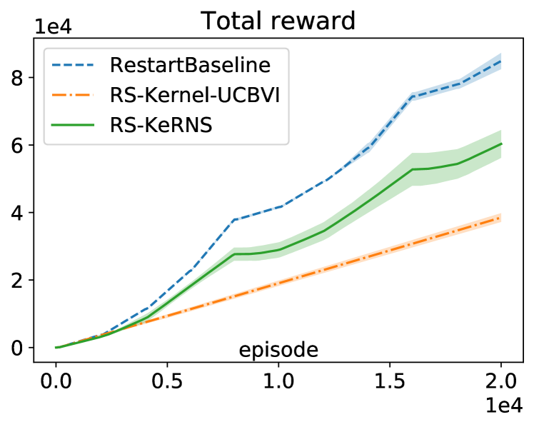
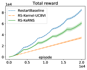
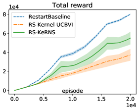
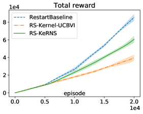
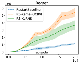
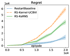
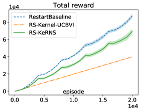
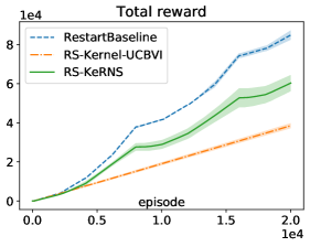
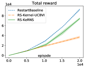
Taking , we used the kernel . We set , , , and ran the algorithm for episodes. KeRNS was compared to two baselines: (i) Kernel-UCBVIcombined with representative states, that we call RS-Kernel-UCBVI, which is designed for stationary environments. This corresponds to RS-KeRNS with , that is, ; (ii) A restart-based algorithm, called RestartBaseline, which is implemented as RS-Kernel-UCBVI, but it has full information about when the environment changes, and, at every change, it restarts its reward estimator and its bonuses. We can see that, as expected, RS-KeRNS outperforms RS-Kernel-UCBVI, which was not designed for non-stationary environments, and is able to “track” the behavior of the restart-based algorithm which has full information about how the environment changes. In Appendix I, we give more details about the experimental setup and provide more experiments, varying the period of changes in the MDP and the kernel function.
5 Proof Outline
We now outline the proof of Theorem 1 assuming, for simplicity, that the rewards are known.
Bias due to non-stationarity
To bound the bias, we introduce an average MDP with transitions :
where are the true transitions at time . We prove that, for any -Lipschitz function bounded by , (Corollary 2):
where the term is defined as
Concentration
Using concentration inequalities for weighted sums, we prove that is close to the average transition using Hoeffding- and Bernstein-type inequalities (lemmas 5, 6, 7, and 8), and define an event where our confidence sets hold (Lemma 9), such that . For instance, Lemma 5 gives us
which explains the form of the exploration bonuses.
Upper bound on the true value function
On the event , we show that (Lemma 10):
where the term is the sum of defined above, and a similar term representing the bias in the reward estimation.
Regret bounds
Let be the state-action pair among the previously visited ones that is the closest to :
We show that (see proof of Lemma 11):
Thus, to simplify the outline, for all , we assume that and add to the final regret bound. On the event , we prove that the regret of KeRNS is bounded by (lemmas 11 and 12):
where we omitted factors involving and (which depend on the type of bound considered, or ), and martingale terms (which are bounded by with probability at least ).
Finally, in Corollary 5, we prove that the bias is bounded by
6 Conclusion
In this paper, we introduced and analyzed KeRNS, the first algorithm for continuous MDPs with dynamic regret guarantees in changing environments. Building upon previous work on using representative states for kernel-based RL, we proposed RS-KeRNS, a practical version of KeRNS that runs in constant time per episode. Moreover, we provide the first analysis that quantifies the trade-off between the regret and the computational complexity of this approach. In discrete environments, our regret bound matches the existing lower bound for multi-armed bandits in terms of the number of episodes and the variation of MDP, whereas finding a lower bound in continuous environments remains an open problem.
We believe that the ideas introduced in this paper might be useful for large-scale problems. Indeed, we provide stronger online guarantees for practical kernel-based RL, which has already been shown to be empirically successful in medium-scale environments () (Kveton and Theocharous,, 2012; Barreto et al.,, 2016), and we show that kernel-based RL is naturally suited to tackle non-stationarity. In larger dimension, kernel-based exploration bonuses have been recently shown to enhance exploration in RL for Atari games (Badia et al.,, 2020), and our approach might inspire the design of bonuses for high-dimensional non-stationary environments.
Acknowledgements
The research presented was supported by European CHIST-ERA project DELTA, French Ministry of Higher Education and Research, Nord-Pas-de-Calais Regional Council, French National Research Agency project BOLD (ANR19-CE23-0026-04), FMJH PGMO project 2018-0045, and the SFI Sachsen-Anhalt for the project RE-BCI ZS/2019/10/102024 by the Investitionsbank Sachsen-Anhalt.
References
- Auer et al., (2019) Auer, P., Gajane, P., and Ortner, R. (2019). Adaptively tracking the best bandit arm with an unknown number of distribution changes. In Conference on Learning Theory, pages 138–158.
- Azar et al., (2017) Azar, M. G., Osband, I., and Munos, R. (2017). Minimax regret bounds for reinforcement learning. In Proceedings of the 34th International Conference on Machine Learning-Volume 70, pages 263–272. JMLR. org.
- Badia et al., (2020) Badia, A. P., Sprechmann, P., Vitvitskyi, A., Guo, D., Piot, B., Kapturowski, S., Tieleman, O., Arjovsky, M., Pritzel, A., Bolt, A., and Blundell, C. (2020). Never give up: Learning directed exploration strategies. In International Conference on Learning Representations.
- Barreto et al., (2016) Barreto, A. M., Precup, D., and Pineau, J. (2016). Practical kernel-based reinforcement learning. The Journal of Machine Learning Research, 17(1):2372–2441.
- Barto et al., (1995) Barto, A. G., Bradtke, S. J., and Singh, S. P. (1995). Learning to act using real-time dynamic programming. Artificial intelligence, 72(1-2):81–138.
- Besbes et al., (2014) Besbes, O., Gur, Y., and Zeevi, A. (2014). Stochastic multi-armed-bandit problem with non-stationary rewards. In Advances in neural information processing systems, pages 199–207.
- Bubeck et al., (2011) Bubeck, S., Munos, R., Stoltz, G., and Szepesvári, C. (2011). X-armed bandits. Journal of Machine Learning Research, 12:1587–1627.
- Chen et al., (2019) Chen, Y., Lee, C.-W., Luo, H., and Wei, C.-Y. (2019). A new algorithm for non-stationary contextual bandits: Efficient, optimal and parameter-free. In Conference on Learning Theory, pages 696–726. PMLR.
- Cheung et al., (2020) Cheung, W. C., Simchi-Levi, D., and Zhu, R. (2020). Reinforcement learning for non-stationary Markov decision processes: The blessing of (More) optimism. In Proceedings of the 37th International Conference on Machine Learning.
- Choi et al., (2000) Choi, S. P., Yeung, D.-Y., and Zhang, N. L. (2000). Hidden-mode markov decision processes for nonstationary sequential decision making. In Sequence Learning, pages 264–287. Springer.
- Csáji and Monostori, (2008) Csáji, B. C. and Monostori, L. (2008). Value function based reinforcement learning in changing markovian environments. Journal of Machine Learning Research, 9(Aug):1679–1709.
- Dann et al., (2017) Dann, C., Lattimore, T., and Brunskill, E. (2017). Unifying pac and regret: Uniform pac bounds for episodic reinforcement learning. In Advances in Neural Information Processing Systems, pages 5713–5723.
- Dick et al., (2014) Dick, T., Gyorgy, A., and Szepesvari, C. (2014). Online learning in markov decision processes with changing cost sequences. In International Conference on Machine Learning, pages 512–520. PMLR.
- Domingues et al., (2020) Domingues, O. D., Ménard, P., Pirotta, M., Kaufmann, E., and Valko, M. (2020). Regret Bounds for Kernel-Based Reinforcement Learning. arXiv e-prints, page arXiv:2004.05599.
- Efroni et al., (2019) Efroni, Y., Merlis, N., Ghavamzadeh, M., and Mannor, S. (2019). Tight regret bounds for model-based reinforcement learning with greedy policies. In Advances in Neural Information Processing Systems, pages 12203–12213.
- Even-Dar et al., (2009) Even-Dar, E., Kakade, S. M., and Mansour, Y. (2009). Online markov decision processes. Mathematics of Operations Research, 34(3):726–736.
- Gajane et al., (2018) Gajane, P., Ortner, R., and Auer, P. (2018). A sliding-window algorithm for markov decision processes with arbitrarily changing rewards and transitions. arXiv preprint arXiv:1805.10066.
- Garivier and Moulines, (2011) Garivier, A. and Moulines, E. (2011). On Upper-Confidence Bound Policies For Switching Bandit Problems. In Algorithmic Learning Theory (ALT), pages 174–188. PMLR.
- Jaksch et al., (2010) Jaksch, T., Ortner, R., and Auer, P. (2010). Near-optimal regret bounds for reinforcement learning. Journal of Machine Learning Research, 11(Apr):1563–1600.
- Jin et al., (2018) Jin, C., Allen-Zhu, Z., Bubeck, S., and Jordan, M. I. (2018). Is Q-learning provably efficient? In Advances in Neural Information Processing Systems, pages 4863–4873.
- Kleinberg et al., (2019) Kleinberg, R., Slivkins, A., and Upfal, E. (2019). Bandits and experts in metric spaces. Journal of the ACM (JACM), 66(4):1–77.
- Kocsis and Szepesvári, (2006) Kocsis, L. and Szepesvári, C. (2006). Discounted UCB. In 2nd PASCAL Challenges Workshop.
- Kveton and Theocharous, (2012) Kveton, B. and Theocharous, G. (2012). Kernel-based reinforcement learning on representative states. In Twenty-Sixth AAAI Conference on Artificial Intelligence.
- Lecarpentier and Rachelson, (2019) Lecarpentier, E. and Rachelson, E. (2019). Non-stationary markov decision processes, a worst-case approach using model-based reinforcement learning. In Advances in Neural Information Processing Systems, pages 7214–7223.
- Li and Li, (2019) Li, Y. and Li, N. (2019). Online learning for markov decision processes in nonstationary environments: A dynamic regret analysis. In 2019 American Control Conference (ACC), pages 1232–1237. IEEE.
- Lykouris et al., (2019) Lykouris, T., Simchowitz, M., Slivkins, A., and Sun, W. (2019). Corruption robust exploration in episodic reinforcement learning. arXiv preprint arXiv:1911.08689.
- Neu et al., (2013) Neu, G., György, A., Szepesvari, C., and Antos, A. (2013). Online markov decision processes under bandit feedback. IEEE Transactions on Automatic Control, 59(3):676–691.
- Ormoneit and Sen, (2002) Ormoneit, D. and Sen, Ś. (2002). Kernel-based reinforcement learning. Machine Learning, 49(2):161–178.
- Ortner et al., (2019) Ortner, R., Gajane, P., and Auer, P. (2019). Variational regret bounds for reinforcement learning. In Proceedings of the 35th Conference on Uncertainty in Artificial Intelligence.
- Ortner and Ryabko, (2012) Ortner, R. and Ryabko, D. (2012). Online regret bounds for undiscounted continuous reinforcement learning. In Advances in Neural Information Processing Systems, pages 1763–1771.
- Puterman, (2014) Puterman, M. L. (2014). Markov decision processes: discrete stochastic dynamic programming. John Wiley & Sons.
- Russac et al., (2019) Russac, Y., Vernade, C., and Cappé, O. (2019). Weighted linear bandits for non-stationary environments. In Advances in Neural Information Processing Systems, pages 12017–12026.
- Sinclair et al., (2020) Sinclair, S., Wang, T., Jain, G., Banerjee, S., and Yu, C. (2020). Adaptive discretization for model-based reinforcement learning. In Advances in Neural Information Processing Systems, pages 3858–3871.
- Sinclair et al., (2019) Sinclair, S. R., Banerjee, S., and Yu, C. L. (2019). Adaptive discretization for episodic reinforcement learning in metric spaces. Proceedings of the ACM on Measurement and Analysis of Computing Systems, 3(3):1–44.
- Song and Sun, (2019) Song, Z. and Sun, W. (2019). Efficient model-free reinforcement learning in metric spaces. arXiv preprint arXiv:1905.00475.
- Szita et al., (2002) Szita, I., Takács, B., and Lörincz, A. (2002). -mdps: Learning in varying environments. Journal of Machine Learning Research, 3(Aug):145–174.
- Yu and Mannor, (2009) Yu, J. Y. and Mannor, S. (2009). Online learning in markov decision processes with arbitrarily changing rewards and transitions. In 2009 international conference on game theory for networks, pages 314–322. IEEE.
- Zanette and Brunskill, (2019) Zanette, A. and Brunskill, E. (2019). Tighter problem-dependent regret bounds in reinforcement learning without domain knowledge using value function bounds. In Proceedings of the 36th International Conference on Machine Learning.
Appendix
Appendix A Preliminaries
A.1 Notation
Throughout the proof, we use the following notation when omitting constants and logarithmic terms:
Table 2 summarizes the main notations used in the paper and in the proofs.
| Notation | Meaning |
|---|---|
| metric on the state-action space | |
| metric on the state space | |
| -covering number of the metric space | |
| number of episodes | |
| horizon, length of each episode | |
| confidence parameter | |
| kernel bandwidth parameter | |
| kernel temporal decay parameter | |
| kernel temporal window parameter | |
| regularization parameter | |
| , | -covering numbers of and , respectively |
| Lipschitz constants of the rewards, transitions and value functions | |
| kernel function from to | |
| parameterized kernel function from to | |
| constants related to kernel properties, see Assumption 4 | |
| function related to kernel properties, see Assumption 4 | |
| true MDP at episode , with rewards and transitions | |
| empirical MDP built by KeRNS in episode | |
| weight at in at time w.r.t the sample (Def. 1) | |
| normalized version of (Def. 1) | |
| true value functions in episode | |
| value functions computed by KeRNS in episode | |
| value functions computed by RS-KeRNS in episode | |
| sets of representative states, actions and next states, at stage of episode | |
| mapping from to | |
| mapping from to | |
| temporal variation of the rewards and transitions (Def. 3) | |
| temporal variation of the MDP | |
| covering dimension of | |
| covering dimension of | |
| threshold distance to add a new representative state-action pair | |
| threshold distance to add a new representative state | |
| set of -Lipschitz functions from to bounded by | |
| bias in transition estimation at time , (Def. 6) | |
| bias in reward estimation at time (Def. 6) | |
| sum of biases (Def. 6) | |
| good event, on which confidence intervals hold (Lemma 9) | |
| equal to for any |
A.2 Probabilistic model
The interaction between the algorithm and the MDP defines a stochastic process for and , representing the state, the action, the next state and the reward at step of episode . Let be the history of the process up to time .
We define as the -algebra generated by , and denote its corresponding filtration by .
A.3 Exploration Bonuses and Kernel Backward Induction
A reinforcement learning algorithm can be seen as a mapping from the set of possible histories to the set of actions .
For a time , KeRNS performs this mapping in the following way:
-
1.
Build and as in Definition 2, which are -measurable.
-
2.
For each , with ,
-
•
Compute
-
•
Define, for any ,
-
•
-
3.
Choose the action .
Notice the algorithmic structure of KeRNS is the same as Kernel-UCBVI (Domingues et al.,, 2020). However, KeRNS uses non-stationary kernels to be able to adapt to changing environments.
It can be checked that Algorithm 3 returns the functions described above.
The exploration bonus is defined below:
Appendix B Proof Outline
In this section, we outline the proof of the regret bound of RS-KeRNS (Theorem 2).
B.1 Theorem 2
To prove the regret bound in Theorem 2 for RS-KeRNS, we consider the kernel:
for a given function . In each episode , RS-KeRNS has build representative sets of states , actions and next states , for each . We define of the projections:
from any to their representatives.
Let . In episode , RS-KeRNS computes the following estimate of the rewards
and the following estimate of the transitions
which are similar to the estimates that would be computed by KeRNS, but using the projections and to the representative states and actions. The values of and are defined for all , but they only need to be stored for , which corresponds to storing a finite representation of the MDP. The exploration bonuses of RS-KeRNS are defined similarly:
We prove that the estimates used by RS-KeRNS are close to the ones used by KeRNS up to bias terms. Then, this result is used to prove that the regret bound of RS-KeRNS is the same as KeRNS, but adding a bias term multiplied by the number of episodes. For any with and , we show that (consequence of Lemma 18):
and similar bounds are obtained for the rewards (Lemma 19) and the exploration bonuses (Lemma 20). This allows us to prove that the regret of RS-KeRNS is bounded as (theorems 5 and 6)
If we choose , the estimators used by RS-KeRNS can be updated online. Indeed, as detailed in Appendix G, we can related the estimates at time to the ones at time :
One issue that we need to solve is that , and were not necessarily computed before episode . This happens when is a new representative state-action pair added in episode . In Section G.2, we show that this can be easily handled by defining some auxiliary quantities that can be updated online and that can be used to initialize the values , and when necessary, with little overhead to the runtime of the algorithm.
B.2 Optimized Kernel Parameters and Regret Bounds
| condition | bound | regret | |||
|---|---|---|---|---|---|
Appendix C Handling the bias due to non-stationarity
Proof.
The result is straightforward when . Assuming , we have
where in the first inequality we used by Assumption 4 that
By symmetry, we obtain
which concludes the proof. ∎
Appendix D Concentration
In this Section, we provide confidence intervals that will be used to prove our regret bounds. The main concentration results are presented in Lemma 9, which defines an event where all the confidence intervals hold, and we show that .
D.1 Concentration inequalities for weighted sums
We reproduce here the concentration inequalities for weighted sums proved by Domingues et al., (2020), which we will need.
Lemma 3 (Hoeffding type inequality (Domingues et al.,, 2020)).
Consider the sequences of random variables and adapted to a filtration . Assume that, for all , is measurable and for all .
Let and , and assume almost surely for all . Then,for any , with probability at least , for all ,
Proof.
See Lemma 2 of Domingues et al., (2020). ∎
Lemma 4 (Bernstein type inequality (Domingues et al.,, 2020)).
Consider the sequences of random variables and adapted to a filtration . Let
Assume that, for all , (i) is measurable, (ii) , (iii) almost surely, (iv) there exists such that almost surely. Then, for all , with probability at least , for all ,
Proof.
See Lemma 3 of Domingues et al., (2020). ∎
D.2 Hoeffding-type concentration inequalities
Proof.
Let . For fixed , we have
Bounding ➀ (martingale term)
Let . From Lemma 3, we have, for a fixed tuple ,
with probability at least , since is a martingale difference sequence with respect to .
From Lemma 24, we verify that the functions
are Lipschitz continuous, with Lipschitz constants bounded by and , respectively. Let be a -covering of . Using the Lipschitz continuity of the functions above and a union bound over and over , we have
for all with probability at least .
Bounding ➁ (spatial bias term)
We have
| ➁ | |||
Putting together the bounds for ➀ and ➁ concludes the proof. ∎
Proof.
Almost identical to the proof of Lemma 5, except for the fact that the rewards are bounded by instead of . ∎
Covering
Now let be a -covering of . Using the fact that the function is 2-Lipschitz with respect to , we do a union bound over to obtain
for all and all , with probability at least , since the -covering number of is bounded by , by Lemma 5 of Domingues et al., (2020).
Covering
By Lemma 24, the functions
are -Lipschitz and , respectively, with respect to the distance . Let be a covering of . Using the continuity of the functions above, a union bound over gives us999see, for instance, Lemma 6 of Domingues et al., (2020).
for all , all and all , with probability at least
and a union bound over concludes the proof. ∎
D.3 Bernstein-type concentration inequality
Proof.
We have
Bounding ➁ (spatial bias term)
As in the proof of Lemma 5, we can show that
| ➁ |
Bounding the martingale term (➀) with a Bernstein-type inequality
Notice that is bounded by and
The conditional variance of is bounded as follows
which we use to bound its weighted average
where, in the last inequality, we used Lemma 23.
Let . Let . By Lemma 4, we have
with probability at least , since, for a fixed , is a martingale difference sequence with respect to . Using the fact that for all ,
Covering of
Covering of
The bounds for ➀ and ➁ give us
The -covering number of with respect to the infinity norm is bounded by , by Lemma 5 of Domingues et al., (2020). The functions and are -Lipschitz with respect to . Consequently, with probability at least
for all and for all , we have
which concludes the proof. ∎
D.4 Good event
Appendix E Upper bound on true value function
In this section, we show that the true value functions can be upper bounded by the value functions computed by KeRNS plus a bias term. This result will be used to upper bound the regret in the next section.
Proof.
We proceed by induction on . For , both quantities are zero, so the inequality is trivially verified. Now, assume that it is true for and let’s prove it for .
From the induction hypothesis, we have . Indeed,
and, since , we have
From the definition of the algorithm, we have
where . Hence,
The term is lower bounded as follows
by Corollary 2 and the fact that on .
Similarly, for the term , we have
which gives us
Consequently, for all and all , we have
since is -Lipschitz . Which implies the result
∎
Proof.
For any ,
where we used the fact that, for any , we have . ∎
Appendix F Regret bounds
Using the results proved in the previous sections, we are now ready to prove our regret bounds. We first start by proving that the regret is bounded by sums involving , and bias terms. Then, we provide upper bounds for these sums, which result in the final regret bounds.
In Theorem 1, we prove two regret bounds, and . Here, we refer to as a UCRL-type regret bound and to as a UCBVI-type bound, due to the technique used to bound the difference between and . Making an analogy with finite MDPs, in UCRL (Jaksch et al.,, 2010), a term analogous to is bounded (as in Lemma 7), whereas in UCBVI (Azar et al.,, 2017), the term is bounded (as in Lemma 5).
Proof.
Definition 8.
For any , let be defined as
that is, the state-action pair in the history that is the closest to .
F.1 Regret bound in terms of the sum of exploration bonuses (UCRL-type)
Proof.
Regret decomposition On , we upper bound using the following decomposition:
Now, we bound each term - separately.
Term :
Term : From Assumption 2, for any -Lipschitz function, the mapping is -Lipschitz . Consequently,
where
is a martingale difference sequence with respect to bounded by .
Putting together the bounds for - and using the definition of the bonuses , we obtain
where the constant in front of is exact (i.e., not omitted by ).
Let . The inequality above implies
| (2) |
Now, we bound in terms of , which will be later used to bound in terms of . On , we have
The inequality above, combined with (2) yields
Let be the complement of . Since , we have
This yields
Using Corollary 4, we obtain
For each , the number of episodes where the event occurs is bounded by . Hence, we can bound the sum
We conclude the proof by recalling the definition and using the fact that is a martingale difference sequence with respect to bounded by . ∎
F.2 Regret bound in terms of the sum of exploration bonuses (UCBVI-type)
Proof.
The proof follows the one of Proposition 5 of Domingues et al., (2020). The key difference is that we need to handle the temporal bias. In particular, is not an upper bound on due to the temporal bias, which makes our proof slightly more technical by introducing (see Cor. 3) when applying the Bernstein-type concentration of Lemma 8.
Regret decomposition
We use the same regret decomposition as in the proof of Lemma 11. The terms and are bounded in the same way, but we handle the term differently.
Term : To bound this term, we use corollaries 2 and 3:
where we also used the definition of and the fact that the function is -Lipschitz , from Assumption 2. Now, since
and , we have
Using again Corollary 3, we have
which gives us, since ,
where we omit constants. Notice, however, that there are no constants omitted in the term .
Putting together the bounds for -, we obtain
where the constant in front of is exact (i.e., not omitted by ).
F.3 Bounding the sum of bonuses and bias
Proof.
We have
∎
Proof.
Proof.
Definition 9.
Consider a -covering of , . We define a partition such that
with ties broken arbitrarily.
Proof.
Proof.
Here, we define the constant as , since by Assumption 4.
Bounding the sum
Bounding the sum
∎
F.4 Final regret bounds
F.4.1 UCRL-type regret bounds
Proof.
Proof.
Immediate consequence of Theorem 3 and the fact that and . ∎
F.4.2 UCBVI-type regret bounds
Proof.
Proof.
Immediate consequence of Theorem 4 and the fact that and . ∎
Appendix G RS-KeRNS: An efficient version of KeRNS using representative states
RS-KeRNS is described in Algorithm 4, which uses a backward induction on representative states (Algorithm 5) and updates the model online (algorithms 6 and 7). In this section, we introduce the main definitions used by RS-KeRNS, and we analyze its runtime and regret.
G.1 Definitions
In each episode and for each , RS-KeRNS keeps and updates sets of representative states , actions , and next-states , with cardinalities and , respectively. These sets are built using the data observed up to episode . We define the following projections:
where we also assume to have access to the metric . The definitions below introduce the kernel function and the estimated MDP used by RS-KeRNS.
At step , RS-KeRNS needs to store the quantities in Def. 11 only for the representatives in and . We will show that, using the auxiliary quantities defined below, the values of , and can be updated online in time per episode .
The following Lemma will be necessary in order to derive online updates.
Proof.
It is an immediate consequence of the definitions. For instance,
∎
G.2 Online updates & runtime
Assume that we observed a transition at time , updated the representative sets, and mapped the transition to the representatives . We wish to update the estimated MDP given in Def. 11, which, at step , are only stored for in and .
The auxiliary quantities (Def. 12) are updated as:
We need to update , and for all . The update rule will depend on whether the is a new representative state-action pair (included in episode ) or it was visited before episode . These two cases are studied below.
Case 1: and
This means that the representative state-action pair was added at time . In this case, for all , the quantities , and can be initialized using equations (29), (54) and (71). This is done in time and can happen, at most, for one pair : the one that was newly added. Therefore, we have a total per-episode runtime of taking this case into account.
Case 2:
This means that the representative state-action pair was added before episode , which implies that . Hence,
This implies that, for a fixed , the quantity can be updated in time, assuming that the mapping was previously computed (this mapping is only computed once for all the updates, and takes time).
Now, notice that
where we used again the fact that, in this case, . Hence, similarly to , the quantity can be updated in time. A similar reasoning shows that can be updated, for all , in time:
Summary
Every time a new transition is observed at time , the estimators for all must be updated. For a given representative , the updates can be done in time if it has been observed before episode (case 2). This results in a total runtime, per episode, of for all the representatives observed before episode . If the representative has not been observed before episode (case 1), the updates require time, and this can happen, at most, for one state-action pair at each time . Hence, the total runtime required for the updates is per episode.
G.3 Regret analysis
The regret analysis of RS-KeRNS is based on the following result, which is a corollary of Lemma 25, and is used to bound the bias introduced by using representative states.
Proof.
We use Corollary 10 to bound the difference between the estimators and the bonuses of KeRNS, , and the ones of RS-KeRNS, .
Proof.
To simplify the notations, let for . We have
where ➀ and ➁ are defined and bounded below. First,
| ➀ | |||
by using the fact that is -Lipschitz and Corollary 10.
To bound ➁, let and , for . Using again the fact that is -Lipschitz and Corollary 10, we obtain
| ➁ | |||
By the construction of the algorithm, , , and , which concludes the proof. ∎
Proof.
Proof.
To simplify the notations, let for . Using definitions 5, 10, and 11, we have
Using Corollary 10, we obtain
| ➀ | |||
Similarly, Corollary 10 yields
| ➁ | |||
By the construction of the algorithm, and , which concludes the proof. ∎
Proof.
Notice that, although is only computed for the representative state-action pairs, it is defined for any as
We claim that
First, , since , we have . Second, for any , there exists such that , which implies that .
Proof.
We proceed by induction on . Let
For , , and the claim holds.
Now, assume that the claim is true for . In this case, we have, for any ,
where we used induction hypothesis and the fact that, for any , we have (Fact 1).
For any with , we have
where, in the last line, we used the induction hypothesis and lemmas 18, 19 and 20.
By the construction of RS-KeRNS, we have . Consequently,
Now, take an arbitrary . By Lemma 21,
and, by definition,
we obtain, for any ,
which concludes the proof. ∎
Proof.
Let be the policy followed by RS-KeRNS in episode and let
Regret decomposition
Consider the following decomposition, also used in the proof of Lemma 11:
We will use the following results, which are a consequence of Lemmas 18, 19 and 20 and the fact that :
and, for any function that is -Lipschitz and bounded by ,
Now, we bound each term .
Term :
Term : From Assumption 2, for any -Lipschitz function, the mapping is -Lipschitz . Consequently,
where
is a martingale difference sequence with respect to bounded by .
Putting together the bounds for - and using the definition of the bonuses , we obtain
where the constant in front of is exact (i.e., not omitted by ).
Now, we follow the same arguments as in the proof of Lemma 11. Consider the event . The inequality above gives us
| (88) | ||||
| (89) |
Let be the complement of . Using the inequality above combined with (89), and the fact that , we obtain
| (192) | ||||
| (201) | ||||
| (210) | ||||
Consequently,
Now, as in the proof of Lemma 11, we show that
Recall the definition and the fact that is a martingale difference sequence with respect to bounded by . Then, as in the proof of Theorem 3, we obtain
with probability at least . ∎
Proof.
We use the same regret decomposition as in the proof of Theorem 5, but the term is bounded differently (as in Lemma 12).
Using Lemma 18, Lemma 22, and the same arguments as in the proof of Lemma 12, we have
where, in the last line, we used the fact that and that by Lemma 22.
Putting together the bounds for and using the same arguments as in the proof of Theorem 5, especially the inequalities (89), (167) and (192), we obtain
where is a martingale difference sequence with respect to bounded by .
Then, as in the proof of Theorem 4, we obtain
with probability at least . ∎
Appendix H Technical Lemmas
Lemma 23 (adapted from Domingues et al., (2020)).
Consider a sequence of non-negative real numbers and let satisfy Assumption 4. For a given , let
for . Then, we have
Proof.
For completeness, we reproduce here the proof of Lemma 7 of Domingues et al., (2020), which also applies to our setting. We split the sum into two terms:
From Assumption 4, we have . Hence, , since .
We want to find such that:
which implies, for , that .
Let . Reformulating, we want to find a value such that for all . Let . If , we have:
as we wanted.
Now, is equivalent to . Therefore, we take , which gives us
Finally, we obtain:
∎
Lemma 24.
Let be a kernel that satisfies Assumption 4. Let and be functions from to defined as
Then, for any , we have
Proof.
From Assumption 4, the function is -Lipschitz , which yields
The proofs for and are analogous. For , we also use the fact that the function is -Lipschitz . ∎
Lemma 25.
Let and be functions from to defined as
where is an arbitrary function bounded by . Then, for any , we have
Proof.
We use the fact that, for any differentiable ,
We have
which implies, by Lemma 23,
The proofs for and are analogous. ∎
Lemma 26 (value functions are Lipschitz continuous).
Proof.
This fact is proved in Lemma 4 of Domingues et al., (2020) and also in Proposition 2.5 of Sinclair et al., (2019). For completeness, we also present a proof here.
We proceed by induction. For , which is -Lipschitz by Assumption 2. Also,
| (211) | ||||
| (212) |
which verifies the induction hypothesis for , since we can invert the roles of and to obtain .
Fact 1 (small useful result).
Proof.
Since , we have
where we used the fact that . By symmetry, . which gives us the result. ∎
Appendix I Experiments
I.1 Setup
We consider a continuous MDP whose state-space is the unit ball in with four actions, representing a move to the right, left, up or down. Each action results in a displacement of in the corresponding direction, plus a Gaussian noise, in both directions, of standard variation . The agent starts at . Let and . We consider the following mean reward function:
Every episodes, the coefficients are changed, which impact the optimal policy.
Taking , we tested the Gaussian kernel and a higher-order kernel . We set , , , .
We ran the experiment with horizon for episodes. Every episodes, the coefficients were changed, according to Table 4.
| episode / | ||||
|---|---|---|---|---|
We took and used the following simplified exploration bonuses:
| (213) |
where the factor was chosen in order to ensure that the baseline is able to learn a good policy in less than episodes, i.e., before there is a change in the environment.
Additionally, to take into account the fact that the Lipschitz constant is rarely known in practical problems, we replaced the interpolation step (line 8 of Alg. 5) by a nearest-neighbor search in the representative states:
I.2 Results
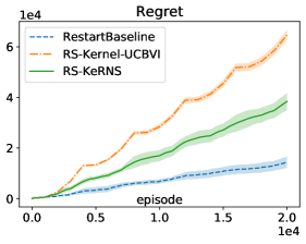
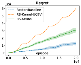
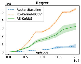
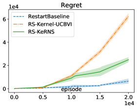
Figures 2 and 3 show the total reward and the regret of RS-KeRNS compared to baselines for the two choices of kernel function (Gaussian and 4-th order kernel), for 3 different values of , which is determined by the period of changes in the MDP (the reward changes every episodes).
In all experiments we observe that Kernel-UCBVI is not able to adapt to the changes in the environment, whereas RS-KeRNS is able to track the behavior of the baseline RestartBaseline which knows when the changes happen and resets the reward estimator when there is a change.