Line-Up Elections:
Parallel Voting with Shared Candidate Pool

Abstract

We introduce the model of line-up elections which captures parallel or sequential single-winner elections with a shared candidate pool. The goal of a line-up election is to find a high-quality assignment of a set of candidates to a set of positions such that each position is filled by exactly one candidate and each candidate fills at most one position. A score for each candidate-position pair is given as part of the input, which expresses the qualification of the candidate to fill the position. We propose several voting rules for line-up elections and analyze them from an axiomatic and an empirical perspective using real-world data from the popular video game FIFA.

Keywords— Single-winner voting, Multi-winner voting, Assignment problem,
        Axiomatic analysis, and Empirical analysis.

1 Introduction

Before the start of the soccer World Cup 2014, Germany’s head coach Joachim Löw had problems to find an optimal team formation. Due to several injuries, Löw was stuck without a traditional striker. He decided to play with three offensive midfielders instead, namely, Müller, Özil, and Götze. However, he struggled to decide who of the players should play in the center, on the right, and on the left. At the final coaching meeting, he surveyed the opinions of ten coaching assistants asking for each of the candidates, “Is this candidate suitable to play on the left/in the center/on the right?”. Coaching assistants were allowed to approve an arbitrary subset of candidate-position pairs. He got answers resulting in the following numbers of approvals for each candidate-position pair:

	Left	Center	Right
Müller	5	10	9
Özil	3	8	5
Götze	4	7	4

After collecting the results, some of the coaches argued that Müller must play in the center, as everyone agreed with this. Others argued that Müller should play on the right, as otherwise this position would be filled by a considerably less suitable player. Finally, someone pointed out that Müller should play on the left, as this was the only possibility to fill the positions such that every position gets assigned a player approved by at least half of the coaches.

The problem of assigning Müller, Özil, and Götze can be modeled as three parallel single-winner elections with a shared candidate pool, where every candidate can win at most one election and each voter is allowed to cast different preferences for each election. In our example, the coaches are the voters, the players are the candidates and the three locations on the field are the positions. Classical single-winner voting rules do not suffice to determine the winners in such settings, as a candidate may win multiple elections. Also multi-winner voting rules cannot be used, as a voter can asses the candidates differently in different elections. Other examples of parallel single-winner elections with a shared candidate pool include a company that wants to fill different positions after an open call for applications, a cooperation electing an executive board composed of different positions, and a professor who assigns students to projects.

In this paper, we introduce a framework for such settings: In a line-up election, we get as input a set of candidates, a set of positions, and for each candidate-position pair a score expressing how suitable this candidate is to win the election for this position. The goal of a line-up election is to find a “good” assignment of candidates to positions such that each position gets assigned exactly one candidate and each candidate is assigned at most once. There exist multiple possible sources of the scores. For instance, a variety of single-winner voting rules aggregate preference profiles into single scores for each candidate and then select the candidate with the highest score as the winner of the given election. Examples of such rules include Copeland’s voting rule, where the score of a candidate is the number of her pairwise victories minus the number of her pairwise defeats, positional scoring rules, or Dodgson’s voting rule. Thus, line-up elections offer a flexible framework that can be built upon a variety of single-winner voting rules.

Our Contributions.

This paper introduces line-up elections—parallel single-winner elections with a shared candidate pool—and initiates a study thereof. After stating the problem formally, we propose two classes of voting rules, sequential and OWA-rules. Sequential rules fill positions in some order—which may depend on the scores—and select the best still available candidate for a given position. In the versatile class of OWA-rules, a rule aims at maximizing some ordered weighted average (OWA) of the scores of the assigned candidate-position pairs. We highlight seven rules from these two classes. Subsequently, inspired by work on voting, we describe several desirable axioms for line-up voting rules and provide a comprehensive and diverse picture of their axiomatic properties. We complement this axiomatic analysis by empirical investigations on data from the popular soccer video game FIFA [10] and synthetic data.

As our model considers multiple, parallel single-winner elections, it can be seen as an extension of single-winner elections; indeed, we can view the scores of candidates for a position as obtained from some voting rule [2, 8, 29]. It reduces to multi-winner voting [13] if every voter casts the same vote in all elections. Most of our proposed axioms are generalizations of axioms studied in those settings [4, 11, 29]. Previously, committee elections where the committee consists of different positions were rarely considered. Aziz and Lee [6] studied multi-winner elections where a given committee is partitioned into different sub-committees and each candidate is suitable to be part of some of these sub-committees.

We defer several details of many discussions and proofs to the appendix.

2 Our Model

In a line-up election $E$, we are given a set of $m$ candidates $C=\{c_{1},\dots,c_{m}\}$ and $q$ positions $P=\{p_{1},\dots,p_{q}\}$ with $m\geq q$, together with a score matrix $\mathbf{S}\in\mathbb{Q}^{m\times q}$. For $i\in[m]$ and $j\in[q]$, $\mathbf{S}_{i,j}$ is the score of candidate $c_{i}$ for position $p_{j}$, which we denote as $\operatorname{score}_{p_{j}}(c_{i})$. An outcome of $E$ is an assignment of candidates to positions, where each position is assigned exactly one candidate and each candidate gets assigned to at most one position. We call an outcome a line-up $\pi$ and write, for a position $p\in P$, $\pi_{p}\in C$ to denote the candidate that is assigned to position $p$ in $\pi$. We write a line-up $\pi$ as a $q$-tuple $\pi=(\pi_{p_{1}},\dots\pi_{p_{q}})\in C^{q}$ with pairwise different entries.

For a candidate-position pair $(c,p)\in C\times P$, we say that $(c,p)$ is assigned in $\pi$ if $\pi_{p}=c$ and write $(c,p)\in\pi$. Moreover, for an outcome $\pi$ and a candidate $c$, let $\pi(c)\in P\cup\{\square\}$ be the position that $c$ is assigned to in $\pi$; that is, $\pi(c)=p$ if $\pi_{p}=c$ and $\pi(c)=\square$ if $c$ does not occur in $\pi$. We write $c\in\pi$ if $\pi(c)\neq\square$, and $c\notin\pi$ otherwise. For a line-up $\pi$ and a subset of positions $P^{\prime}\subseteq P$, we write $\pi|_{P^{\prime}}$ to denote the tuple $\pi$ restricted to positions $P^{\prime}$ and $\pi_{P^{\prime}}$ to denote the set of candidates assigned to positions $P^{\prime}$ in $\pi$. For a position $p\in P$ and line-up $\pi$, we write $\operatorname{score}_{p}(\pi)$ to denote $\operatorname{score}_{p}(\pi_{p})$. Moreover, we refer to $(\operatorname{score}_{p_{1}}(\pi),\dots,\operatorname{score}_{p_{q}}(\pi))$ as the score vector of $\pi$. A line-up voting rule $f$ maps a line-up election $E$ to a set of winning line-ups, where we use $f(E)\subseteq 2^{C^{q}}$ to denote the set of winning line-ups returned by rule $f$ applied to election $E$.

3 Line-Up Elections as Assignment Problems

It is possible to interpret line-up elections as instances of the Assignment Problem, which aims to find a (maximum weight) matching in a bipartite graph. The assignment graph $G$ of a line-up election $(\mathbf{S},C,P)$ is a complete weighted bipartite graph $G=(C\uplus P,E,w)$ with edge set $E:=\{\{c,p\}\mid c\in C\wedge p\in P\}$ and weight function $w(c,p):=\operatorname{score}_{p}(c)$ for $\{c,p\}\in E$. Every matching in the assignment graph which matches all positions induces a valid line-up.

The Assignment Problem and its generalizations have been mostly studied from an algorithmic and fairness perspective [17, 18, 19, 21, 23, 24]. For instance, Lesca et al. [23] studied finding assignments with balanced satisfaction from an algorithmic perspective. They utilized ordered weighted average operators and proved that finding assignments that maximize an arbitrary non-decreasing ordered weighted average is NP-hard (see next section for definitions). One generalization of the Assignment Problem is the Conference Paper Assignment Problem (CPAP), which tries to find a many-to-many assignment of papers to reviewers with capacity constraints on both sides [20]. Focusing on egalitarian considerations, Garg et al. [18] studied finding outcomes of CPAP which are optimal for the reviewer that is worst off, where they break ties by looking at the next worst reviewer. They proved that this task is computationally hard in this generalized setting. In contrast to our work and the work by Lesca et al. [23], Lian et al. [24] employed OWA-operators in the context of CPAP on a different level. Focusing on the satisfaction of reviewers, they studied finding assignments maximizing the ordered weighted average of the values a reviewer gave to her assigned papers and conducted experiments where they compare different OWA-vectors.

In contrast to previous work on the Assignment Problem, we look at the problem through the eyes of voting theorists. We come up with several axiomatic and quantitative properties that are desirable to fulfill by a mechanism if we assume that the Assignment Problem is applied in the context of an election.

4 Voting Rules

As we aim at selecting an individually-excellent line-up, a straightforward approach is to maximize the social welfare, which is determined by the scores of the assigned candidate-position pairs. However, it is not always clear which type of social welfare may be of interest. For example, the overall performance of a line-up may depend on the performance of the worst candidate. This may apply to team sports. Sometimes, however, the performance of a line-up is proportional to the sum of the scores and it does not hurt if some positions are not filled by a qualified candidate. OWA-operators provide a convenient way to express both these goals, as well as a continuum of middle-ground approaches [27].

OWA-rules $\boldsymbol{\mathcal{F}^{\Lambda}}$. For a tuple $a=(a_{1},\dots,a_{k})$ and $i\in[k]$, let $a[i]$ be the $i$-th largest entry of $a$. We call $\Lambda:=(\lambda_{1},\dots,\lambda_{k})$ an ordered weighed-average vector (OWA-vector) and define the ordered weighted average of $a$ under $\Lambda$ as $\Lambda(a_{1},\dots,a_{k}):=\sum_{i\in[k]}\lambda_{i}\cdot a[i]$ [27]. For a line-up $\pi$, we define $\Lambda(\pi)$ as the ordered weighted average of the score vector of $\pi$ under $\Lambda$. That is, $\Lambda(\pi):=\Lambda\big{(}\operatorname{score}_{p_{1}}(\pi),\dots,\operatorname{score}_{p_{q}}(\pi)\big{)}$. The score of a line-up $\pi$ assigned by an OWA-rule $f^{\Lambda}$ is $\Lambda(\pi)$. Rule $f^{\Lambda}$ chooses (possibly tied) line-ups with the highest score.

Among this class of rules, we focus on the following four natural ones, quite well studied in other contexts, such as finding a collective set of items [5, 9, 12, 26]:

• Utilitarian rule $f^{\operatorname{ut}}$: $\Lambda^{\operatorname{ut}}:=(1,\dots,1)$. This corresponds to computing a maximum weight matching in the assignment graph. It is computable in $\mathcal{O}(m^{3})$ time for $m$ candidates [21].

• Egalitarian rule $f^{\operatorname{eg}}$: $\Lambda^{\operatorname{eg}}:=(0,\dots,0,1)$. This corresponds to solving the Linear Bottleneck Assignment Problem, which can be done in $\mathcal{O}(m^{2})$ time for $m$ candidates [17].

• Harmonic rule $f^{\operatorname{har}}$: $\Lambda^{\operatorname{har}}:=(1,\frac{1}{2},\frac{1}{3},\dots,\frac{1}{q})$. The computational complexity of finding a winning line-up under this rule is open. In our experiments, we compute it using Integer Linear Programming (ILP).

• Inverse harmonic rule $f^{\operatorname{ihar}}$: $\Lambda^{\operatorname{ihar}}:=(\frac{1}{q},\frac{1}{q-1},\dots,\frac{1}{2},1)$. While computing the winning line-up for an arbitrary non-decreasing OWA-vector is NP-hard [23], the computational complexity of computing this specific rule is open. We again use an ILP to compute a winning line-up.

Sequential-rules $\boldsymbol{\mathcal{F}^{\operatorname{seq}}}$. OWA-rules require involved algorithms and cannot be applied by hand easily. In practice, humans tend to solve a line-up election in a simpler way, for instance, by determining the election winners one by one. This procedure results in a class of quite intuitive sequential voting rules. A sequential rule is defined by some function $g$ that, given a line-up election $E=(\mathbf{S},C,P)$ and a set of already assigned candidates $C_{\text{as}}$ and positions $P_{\text{as}}$, returns the next position to be filled. This position is then filled by the remaining candidate $C\setminus C_{\text{as}}$ with the highest score on this position. Sequentializing decisions which partly depend on each other has also proven to be useful in other voting-related problems, such as voting in combinatorial domains [22], or in the House Allocation problem in form of the well-known mechanism of serial dictatorship. We focus on the following three linear-time computable sequential rules.

Fixed-order rule $f^{\operatorname{seq}}_{\operatorname{fix}}$. Here, the positions are filled in a fixed order (for simplicity, we assume the order in which the positions appear in the election). The fixed-order sequential rule is probably the simplest way to generalize single-winner elections to the line-up setting and it enables us to make the decisions separately. Moreover, it is not necessary to evaluate all candidates for all positions, which is especially beneficial if evaluating the qualification of a candidate on a position comes at some (computational) cost.

Max-first rule $f^{\operatorname{seq}}_{\operatorname{max}}$. In the max-first rule, at each step the position with the highest still available score is filled. That is, $g(\mathbf{S},C,P,C_{\text{as}},P_{\text{as}}):=\operatorname*{arg\,max}_{p\in P\setminus P_{\text{as}}}\max_{c\in C\setminus C_{\text{as}}}\operatorname{score}_{p}(c)$. This is equivalent to adding at each step the remaining candidate-position pair with the highest score to the line-up. Max-first is intuitively appealing because a candidate who is outstanding at a position is likely to be assigned to it. Notably, this rule is an approximation of the utilitarian rule, as it corresponds to solving the Maximum Weight Matching problem in the assignment graph by greedily selecting the remaining edge with the highest weight. For every possible tie-breaking, this approach is guaranteed to yield a $\frac{1}{2}$-approximation of the optimal solution in polynomial time [3].

Min-first rule $f^{\operatorname{seq}}_{\operatorname{min}}$. In the min-first rule, the position with the lowest score of the most-suitable remaining candidate is filled next. That is, $g(\mathbf{S},C,P,C_{\text{as}},P_{\text{as}}):=\operatorname*{arg\,min}_{p\in P\setminus P_{\text{as}}}\max_{c\in C\setminus C_{\text{as}}}\operatorname{score}_{p}(c).$ The reasoning behind this is that the deciders focus first on filling critical positions where all candidates perform poorly.

	non	Pareto	reasonable	score	position	mono-	line-up
	wasteful	optimal	satisfaction	consistent	consistent	tonicity	enlargement
$f^{\operatorname{ut}}$	S	S	$-$	S	W	S	S
$f^{\operatorname{har}}$	S	S	$-$	$-$	$-$	$-$	$-$
$f^{\operatorname{ihar}}$	S	S	$-$	$-$	$-$	$-$	$-$
$f^{\operatorname{eg}}$	W$\dagger$	W$\dagger$	$-$	$-$	W	$-$$\dagger$	W$\dagger$
$f^{\operatorname{seq}}_{\operatorname{fix}}$	S	W	$-$	W	W	S	S
$f^{\operatorname{seq}}_{\operatorname{max}}$	S	W	S	$-$	W	S	S
$f^{\operatorname{seq}}_{\operatorname{min}}$	S	$-$	$-$	$-$	W	$-$	$-$

Table 1: Overview of axiomatic properties of all studied rules. For each of the axioms, we indicate whether this axiom is strongly satisfied (S), only weakly satisfied (W), or not satisfied at all ($-$). For the egalitarian rule, all entries marked with a $\dagger$ can be improved if a variant of this rule that selects the egalitarian outcome with the highest summed score is used.

5 Axiomatic Analysis of Voting Rules

We propose several axioms and properties that serve as a starting point to characterize and compare the introduced voting rules. We checked all introduced voting rules against all the axioms and collected the results in Table 1 (see Subsection A.3 for all proofs). We will introduce two efficiency and one fairness axiom for line-ups. These definitions extend to voting rules as follows. A voting rule $f$ strongly (weakly) satisfies a given axiom if for each line-up election $E$, $f(E)$ contains only (some) line-ups satisfying the axiom.

Efficiency axioms. As our goal is to select individually-excellent outcomes, we aim at selecting line-ups in which the score of each position is as high as possible. Independent of conflicts between positions, there exist certain outcomes which are suboptimal. For example, it is undesirable if there exists an unassigned candidate that is more suitable for some position than the currently assigned one.

Axiom 1.

Non-wastefulness: In a line-up election $(\mathbf{S},C,P)$, a line-up $\pi$ is non-wasteful if there is no unassigned candidate $c\notin\pi$ and a position $p\in P$ such that $\operatorname{score}_{p}(c)>\operatorname{score}_{p}(\pi)$.

This axiom implies that in the special case of a single position, the candidate with the highest score for the position wins the election. In the context of non-wastefulness, we only examine whether a line-up can be improved by assigning unassigned candidates. However, it is also possible to consider arbitrary rearrangements. This results in the notion of score Pareto optimality.

Axiom 2.

Score Pareto optimality: In a line-up election $(\mathbf{S},C,P)$, a line-up $\pi$ is score Pareto dominated if there exists a line-up $\pi^{\prime}$ such that for all $p\in P$, $\operatorname{score}_{p}(\pi^{\prime})\geq\operatorname{score}_{p}(\pi)$ and there exists a position $p\in P$ with $\operatorname{score}_{p}(\pi^{\prime})>\operatorname{score}_{p}(\pi)$. A line-up is score Pareto optimal if it is not score Pareto dominated.

While all OWA-rules with an OWA-vector containing no zeros are clearly strongly non-wasteful and strongly score Pareto optimal, the egalitarian rule satisfies both axioms only weakly, as this rule selects a line-up purely based on its minimum score. All sequential rules naturally satisfy strong non-wastefulness. Yet, by breaking ties in a suboptimal way, all of them may output line-ups that are not score Pareto optimal. While for the fixed-order rule and the max-first rule at least one winning outcome is always score Pareto optimal, slightly counterintuitively, there exist instances where the min-first rule does not output any score Pareto optimal line-ups.

Fairness axioms. Another criterion to judge the quality of a voting rule is to assess whether positions and candidates are treated in a fair way. The underlying assumption for fairness in this context is that every position should have the best possible candidate assigned. Similarly, from candidates’ perspective, one could argue that each candidate deserves to be assigned to the position for which the candidate is most suitable. In the following, we call a candidate or position for which fairness is violated dissatisfied. Unfortunately, line-ups in which all positions and candidates are satisfied simultaneously may not exist. That is why we consider a restricted fairness property, where we call a candidate-position pair $(c,p)\in\pi$ reasonably dissatisfied in $\pi$ if candidate $c$ has a higher score for $p$ than $\pi_{p}$ and $c$ is either unassigned or $c$’s score for $p$ is higher than for $\pi(c)$.

Axiom 3.

Reasonable satisfaction: A line-up $\pi$ is reasonably satisfying if there are no two positions $p$ and $p^{\prime}$ such that

$$\operatorname{score}_{p}(\pi_{p^{\prime}})>\operatorname{score}_{p}(\pi_{p})\text{ and }\operatorname{score}_{p}(\pi_{p^{\prime}})>\operatorname{score}_{p^{\prime}}(\pi_{p^{\prime}})$$

and there is no candidate $c\notin\pi$ and position $p$ such that $\operatorname{score}_{p}(c)>\operatorname{score}_{p}(\pi_{p}).$

It is straightforward to prove that all winning line-ups under the max-first rule are reasonably satisfying; hence, a reasonably satisfying outcome always exists. Note that it is also possible to motivate reasonable satisfaction as a notion of stability if we assume that candidates and positions are allowed to leave their currently assigned partner to pair up with a new candidate or position. Thus, reasonable satisfaction resembles the notion of stability in the context of the Stable Marriage problem [16].

However, fulfilling reasonable satisfaction may come at the cost of selecting a line-up that is suboptimal for various notions of social welfare. For some $\epsilon>0$, consider an election with $P=\{p_{1},p_{2}\}$, $C=\{a,b\}$, $\operatorname{score}_{p_{1}}(a)=2$, $\operatorname{score}_{p_{2}}(a)=\operatorname{score}_{p_{1}}(b)=2-\epsilon$, and $\operatorname{score}_{p_{2}}(b)=0$. We see that the outcome $(b,a)$ of utilitarian welfare $4-2\epsilon$ maximizes utilitarian social welfare, while the outcome $(a,b)$ of utilitarian welfare $2$ is the only outcome satisfying reasonable satisfaction. Therefore, it is interesting to measure the price of reasonable satisfaction in terms of utilitarian welfare. Analogous to the price of stability [1], we define this as the maximum utilitarian social welfare achievable by a reasonably satisfying outcome, divided by the maximum achievable utilitarian social welfare. The example from above already implies that this price is upper bounded by $\frac{1}{2}$. In fact, this bound is tight, as the max-first rule that only outputs reasonably satisfying line-ups is a $\frac{1}{2}$-approximation of the utilitarian outcome.

Voting axioms. We now formulate several axioms that are either closely related to axioms from single-winner [29] or multi-winner voting [11]. We define all axioms using two parts, (a) and (b). On a high level, condition (a) imposes that certain line-ups should be winning after modifying a line-up election, while condition (b) demands that no other line-ups become (additional) winners after the modifications. If a voting rule only fulfills condition (a), then we say that it weakly satisfies the corresponding axiom. If it fulfills both conditions, then we say that it strongly satisfies the corresponding axiom.

In single-winner and multi-winner voting, the consistency axiom requires that if a voting rule selects the same outcome in two elections (over the same candidate set), then this outcome is also winning in the combined election [28]. We consider a variant of this axiom, adapted to our setting.

Axiom 4.

Score consistency: For two line-up elections $(\mathbf{S},C,P)$ and $(\mathbf{S}^{\prime},C,P)$ with $f(\mathbf{S},C,P)\cap f(\mathbf{S}^{\prime},C,P)\neq\emptyset$ it holds that: a) $f(\mathbf{S},C,P)\cap f(\mathbf{S}^{\prime},C,P)\subseteq f(\mathbf{S}+\mathbf{S}^{\prime},C,P)$ and b) $f(\mathbf{S},C,P)\cap f(\mathbf{S}^{\prime},C,P)\supseteq f(\mathbf{S}+\mathbf{S}^{\prime},C,P).$

The utilitarian rule is the only OWA-rule that satisfies weak (and even strong) score consistency. The fixed-order rule is the only other considered rule that satisfies weak score consistency. For all other rules, it is possible to construct simple two-candidates two-positions line-up elections where this axiom is violated.

We now consider a different way of combining two line-up elections which is special to our setting. In line-up elections, it is possible to combine the set of considered positions: Imagine that we split a line-up election into two sub-elections with the same candidate set in both elections and partly overlapping sets of positions. Assume further that the considered voting rule outputs a winning outcome of the fist sub-election and a winning outcome of the second sub-election such that all shared positions are filled by the same candidates and all non-shared positions by different candidates that do not appear in the other line-up at all. Now, considering the full election on all positions, the union of these outcomes should then be a winning outcome. Formally, we say that two line-ups, $\pi^{\prime}$ defined on $P^{\prime}$ and $\pi^{\prime\prime}$ defined on $P^{\prime\prime}$, are overlapping-disjoint if they assign the same candidates on all positions from $P^{\prime}\cap P^{\prime\prime}$ and a disjoint set of candidates to the other positions. For two overlapping-disjoint line-ups $\pi^{\prime}$ and $\pi^{\prime\prime}$, we write $\pi^{\prime}\cup\pi^{\prime\prime}$ to denote the line-up $\pi^{*}$ combining the two, that is, for all $p\in P^{\prime}\colon\pi^{*}_{p}=\pi_{p}$ and for all $p\in P^{\prime\prime}\colon\pi^{*}_{p}=\pi^{\prime}_{p}$.

Axiom 5.

Position consistency: Let $(\mathbf{S},C,P)$ be a line-up election and $P^{\prime},P^{\prime\prime}\subseteq P$ two subsets of positions with $P^{\prime}\cup P^{\prime\prime}=P$. If there exist two overlapping-disjoint outcomes $\pi^{\prime}\in f(\mathbf{S},C,P^{\prime})$ and $\pi^{\prime\prime}\in f(\mathbf{S},C,P^{\prime\prime})$, then it holds that (a) $\pi^{\prime}\cup\pi^{\prime\prime}\in f(\mathbf{S},C,P)$ and (b) for all $\pi^{*}\in f(\mathbf{S},C,P)$, there exist overlapping-disjoint $\pi^{\prime}\in f(\mathbf{S},C,P^{\prime})$ and $\pi^{\prime\prime}\in f(\mathbf{S},C,P^{\prime\prime})$ such that $\pi^{*}=\pi^{\prime}\cup\pi^{\prime\prime}$.

It is easily possible to construct small instances for all considered voting rules where strong position consistency is violated. However, all rules except the two harmonic rules satisfy the axiom in the weak sense. The harmonic rules fail the axiom because it is possible to exploit the fact that by extending the election, the coefficient by which a score in the line-up is multiplied changes compared to the two sub-elections.

Besides focusing on consistency related considerations, it is also important to examine how the winning line-ups change if the election itself is modified. We start by considering a variant of monotonicity [14].

Axiom 6.

Monotonicity: Let $(\mathbf{S},C,P)$ be a line-up election with a winning line-up $\pi$. Let $(\mathbf{S}^{\prime},C,P)$ be the line-up election obtained from $(\mathbf{S},C,P)$ by increasing $\operatorname{score}_{p}(\pi_{p})$ for some $p$. Then, it holds that (a) $\pi$ is still a winning line-up, that is, $\pi\in f(\mathbf{S}^{\prime},C,P)$, and (b) no new winning line-ups are created, that is, for all $\pi^{\prime}\in f(\mathbf{S}^{\prime},C,P)$ it holds that $\pi^{\prime}\in f(\mathbf{S},C,P)$.

While the utilitarian, fixed-order, and max-first rule all satisfy strong monotonicity, all other rules fail even weak monotonicity. As these negative results are intuitively surprising, we present their proof here.

Proposition 1.

The egalitarian rule $f^{\operatorname{eg}}$, the harmonic rule $f^{\operatorname{har}}$, and the min-first rule $f^{\operatorname{seq}}_{\min}$ all violate weak monotonicity.

Proof.

We present counterexamples for all three rules:

$E_{1}:$ $p_{1}$ $p_{2}$ $a$ $0$ $3$ $b$ $3$ $0$ $c$ $4$ $0$   $E_{2}:$ $p_{1}$ $p_{2}$ $p_{3}$ $a$ $4$ $1$ $0$ $b$ $4.75$ $3$ $0$ $c$ $0$ $0$ $2$   $E_{3}:$ $p_{1}$ $p_{2}$ $a$ 2 1 $b$ 0 0

In $E_{1}$, $(b,a)$ and $(c,a)$ are winning under $f^{\operatorname{eg}}$. However, after increasing $\operatorname{score}_{p_{2}}(a)$ to $4$, $(c,a)$ has an egalitarian score of $4$ and thereby becomes the unique winning line-up. We now turn to election $E_{2}$ and voting rule $f^{\operatorname{har}}$. It is clear that $c$ will be assigned to $p_{3}$ in every outcome. In fact, $(a,b,c)$ is the winning line-up in $E_{2}$, as $\Lambda^{\operatorname{har}}(a,b,c)=1\cdot 4+\frac{1}{2}\cdot 3+\mathbf{\frac{1}{3}\cdot 2}>1\cdot 4.75+\frac{1}{3}\cdot 1+\mathbf{\frac{1}{2}\cdot 2}=\Lambda^{\operatorname{har}}(b,a,c)$. After increasing $\operatorname{score}_{p_{3}}(c)$ to $3$, $(b,a,c)$ becomes the unique winning line-up in $E_{2}$, as $\Lambda^{\operatorname{har}}(a,b,c)=1\cdot 4+\frac{1}{2}\cdot 3+\mathbf{\frac{1}{3}\cdot 3}<1\cdot 4.75+\frac{1}{3}\cdot 1+\mathbf{\frac{1}{2}\cdot 3}=\Lambda^{\operatorname{har}}(b,a,c)$. By the modification, the score of $(b,a,c)$ increases more than the score of $(a,b,c)$, because in $(b,a,c)$ $\operatorname{score}_{p_{3}}(c)$ is multiplied by a larger coefficient. Lastly, considering $f^{\operatorname{seq}}_{\min}$, $(b,a)$ is the unique winning outcome in $E_{3}$. After increasing $\operatorname{score}_{p_{2}}(a)$ to 3, the ordering in which the positions get assigned changes, and thereby, $(a,b)$ becomes the unique winning line-up. ∎

In the context of multi-winner voting, an additional monotonicity axiom is sometimes considered: Committee enlargement monotonicity deals with the behavior of the set of winning outcomes if the size of the committee is increased [7, 11]. We generalize this axiom to our setting in a straightforward way.

Axiom 7.

Line-up enlargement monotonicity: Let $(\mathbf{S},C,P)$ be a line-up election and let $(\mathbf{S}^{\prime},C,P^{\prime})$ with $P^{\prime}=P\cup\{p^{*}\}$ be an election where position $p^{*}$ and the scores of candidates for this position have been added. It holds that (a) for all $\pi\in f(\mathbf{S},C,P)$ there exists some $\pi^{\prime}\in f(\mathbf{S}^{\prime},C,P^{\prime})$ such that $\pi_{P}\subset\pi^{\prime}_{P^{\prime}}$ and (b) for all $\pi^{\prime}\in f(\mathbf{S}^{\prime},C,P^{\prime})$ there exists some $\pi\in f(\mathbf{S},C,P)$ such that $\pi_{P}\subset\pi^{\prime}_{P^{\prime}}$.

Note that line-up enlargement monotonicity does not require that the selected candidates are assigned to the same position in the two outcomes $\pi$ and $\pi^{\prime}$. Despite the fact that this axiom seems to be very natural, neither of the two harmonic rules satisfy it at all. Intuitively, the reason for this is that by introducing a new position, the coefficients in the OWA-vector “shift”. Moreover, surprisingly, the min-first rule also violates the weak version of this axiom. The proof for this consists of a rather involved counterexample (see Theorem 13 in the appendix) exploiting the fact that by introducing a new position, the order in which the positions are filled may change. All other rules, apart from the egalitarian one, satisfy strong line-up enlargement monotonicity; the egalitarian rule satisfies line-up enlargement monotonicity only in the weak sense. We conclude with presenting the proof that the utilitarian rule, $f^{\operatorname{ut}}$, satisfies weak line-up enlargement monotonicity, as the proof nicely illustrates how it is possible to reason about this axiom.

Proposition 2.

The utilitarian rule $f^{\operatorname{ut}}$ satisfies weak line-up enlargement monotonicity.

Proof.

Let $\pi$ be a winning line-up of the initial election $E=(\mathbf{S},C,P)$ and let $\pi^{\prime}$ be a winning line-up of the extended election $E^{\prime}=(\mathbf{S}^{\prime},C,P\cup\{p^{*}\})$ such that there exists a candidate $c\in C$ with $c\in\pi$ and $c\notin\pi^{\prime}$. We claim that it is always possible to construct from $\pi^{\prime}$ a winning line-up $\pi^{*}$ of the extended election such that all candidates from $\pi$ appear in $\pi^{*}$: Initially, we set $\pi^{*}:=\pi^{\prime}$. As long as there exists a candidate $c\in C$ with $c\in\pi$ and $c\notin\pi^{*}$, we set $\pi^{*}_{\pi(c)}:=c$. Let $\widetilde{P}$ be the set of all positions where $\pi^{\prime}$ and $\pi^{*}$ differ. Note that none of the replacements can change the candidate assigned to $p^{*}$. Thus, it holds that $\widetilde{P}\subseteq P$.

Obviously, all candidates from $\pi$ appear in $\pi^{*}$. For the sake of contradiction, let us assume that $\pi^{*}$ is not a winning line-up of the extended election. Consequently, the summed score of $\pi^{*}$ has decreased by the sequence of replacements described above, which implies that the summed scores of candidates on positions from $\widetilde{P}$ is higher in $\pi^{\prime}$ than in $\pi$: $\Lambda^{\operatorname{ut}}(\pi|_{\widetilde{P}})<\Lambda^{\operatorname{ut}}(\pi^{\prime}|_{\widetilde{P}})$. We claim that using this assumption, it is possible to modify $\pi$ such that its utilitarian score increases, which leads to a contradiction, as we have assumed that $\pi$ is a winning line-up. Let $\pi_{\textrm{alt}}$ be a line-up resulting from copying $\pi$ and then replacing all candidates assigned to positions in $\widetilde{P}$ by the candidates assigned to these positions in $\pi^{\prime}$. This is possible as $p^{*}\notin\widetilde{P}$. By our assumption, $\pi_{\textrm{alt}}$ has a higher utilitarian score than $\pi$. It remains to argue that $\pi_{\textrm{alt}}$ is still a valid outcome, that is, every candidate is only assigned to at most one position. This directly follows from the observation that if $p\in\widetilde{P}$ with $\pi^{\prime}_{p}\in\pi$, then at some point during the construction of $\pi^{*}$, $\pi^{\prime}_{p}$ is kicked out of the line-up and is assigned to position $\pi(\pi^{\prime}_{p})$ at some later point, which implies that $\pi(\pi^{\prime}_{p})\in\widetilde{P}$. ∎

Summary. From an axiomatic perspective, the utilitarian rule is probably the most appealing one. Indeed, it satisfies all axioms except weak reasonable satisfaction, which imposes quite rigorous restrictions on every rule fulfilling it. For the egalitarian rule, although this rule is pretty simple, both efficiency axioms are only weakly satisfied and, slightly surprisingly, score consistency and monotonicity are not satisfied at all. As in 1, most of the counterexamples for the egalitarian rule utilize that the OWA-vector of this rule contains some zeros. If one adapts the egalitarian rule such that the egalitarian outcome with the highest summed score is chosen, strong non-wastefulness, strong score Pareto optimality, strong monotonicity, and strong line-up enlargement monotonicity are additionally satisfied. Note that this variant of the egalitarian rule is still computable in polynomial time.

Both harmonic rules are less appealing from an axiomatic perspective because they do not satisfy any of our considered voting axioms. On a high level, as illustrated in 1, this is because the corresponding OWA-vectors consist of multiple different entries. Thereby, some modifications change the coefficients by which the scores are multiplied in some undesirable way. Overall, the contrast between the utilitarian rule and the harmonic rule is quite remarkable because they come both from the same class and work pretty similarly.

Turning to sequential rules, apart from reasonable dissatisfaction, the fixed-order rule outperforms the other two. However, a clear disadvantage of the fixed-order rule is that a returned winning line-up might not be score Pareto optimal. As the max-first rule fulfills all axioms—except score consistency—at least weakly, and it is the only voting rule that is reasonably satisfying, this rule is also appealing if satisfaction of the candidates or positions is an important criterion. The min-first rule, on the other hand, does not weakly satisfy any axiom except non-wastefulness. The reason for this is that in some elections modifying the election changes the order in which the positions are filled. The considerable differences between the max-first and min-first rule are quite surprising, as they first appear to be symmetric.

6 Experiments

In this section, we analyze the proposed rules experimentally. We first describe how we generated our data, and then present and analyze the results.

FIFA data. In the popular video game FIFA 19 [10], 18.207 soccer players have their own avatar. To mimic the quality of a player, experts assessed them on 29 attributes, such as sprint speed, shot power, agility, and heading [15]. From these, the game computes the quality of a player on each possible position, such as left striker or right wing-back etc., in a soccer formation, using a weighted sum of the attribute scores with coefficients depending on the position in question [25]. We used this data to model a coach of a national team $\mathcal{X}$ that wants to find an “optimal” assignment of players with nationality $\mathcal{X}$ to positions in a formation he came up with. This can be modeled as a line-up election.

In soccer, there exist several possible formations consisting of different positions a team can play in. We fixed one formation, that is, a set of ten different positions (see Figure 5 in the appendix for a visualization).

In the generated elections, the candidates are some selected number of players of a given nationality with the highest summed score, the positions are the field positions in a selected soccer formation, and the scores are those assigned by FIFA 19 for the player playing on a particular position. We considered 84 national teams (those with over ten field players in FIFA 19).

Synthetic data. We also generated a synthetic dataset (M2) consisting of $1.000$ line-up elections. Here, every candidate $c$ has a ground qualification $\mu_{c}\in[0.4,0.7]$ and every position $p$ has a difficulty $\alpha_{p}\in[1,2]$ both drawn uniformly at random. For each candidate $c$ and for each position $p$, we sample a basic score $\beta_{c,p}$ from a Gaussian distribution with mean $\mu_{c}$ and standard deviation $0.05$. The score of a candidate-position pair is then calculated as: $\operatorname{score}_{p}(c)=\beta_{c,p}^{\alpha_{p}}$. The intuition behind this is that very talented candidates are presumably not strongly affected by the difficulty of a position, whereas weaker candidates may feel completely overburdened by a difficult position. In addition, we generated another synthetic dataset (M1) that resembles the FIFA data. The description of this model and the results for it are deferred to Subsection B.3 and Subsection B.5.

For both models, we normalized each line-up election by dividing all scores by the maximum score of a candidate-position pair.

Analysis of experimental results. We focus on the case of ten candidates on ten positions, as this is the most relevant scenario in the FIFA setting. However, we also conducted experiments for twenty candidates on ten positions and twenty candidates on twenty positions, where we observed the same trends as in the case presented here (see Subsection B.6 for diagrams). For settings with more candidates than positions, however, the differences between the rules are less visible. In the following, we refer to the (possibly invalid) outcome where every position gets assigned its best candidate as the utopic outcome. To visualize our results, we use violin plots. In a violin plot, the white dot represents the median, the thick bar represents the interquartile range, and the thin line represents the range of the data without outliers. Additionally, a distribution interpolating the data is plotted on both sides of the center.

Comparison of data models. To compare the datasets, we calculated different metrics designed to measure the amount of “competition” in instances. For example, we calculated the difference between the summed score of the utopic outcome and the summed score of a utilitarian outcome (see Subsection B.4 for details). Generally speaking, the M2 model produces instances with more “competition” than the FIFA data which helps us to make the differences between the rules more pronounced.

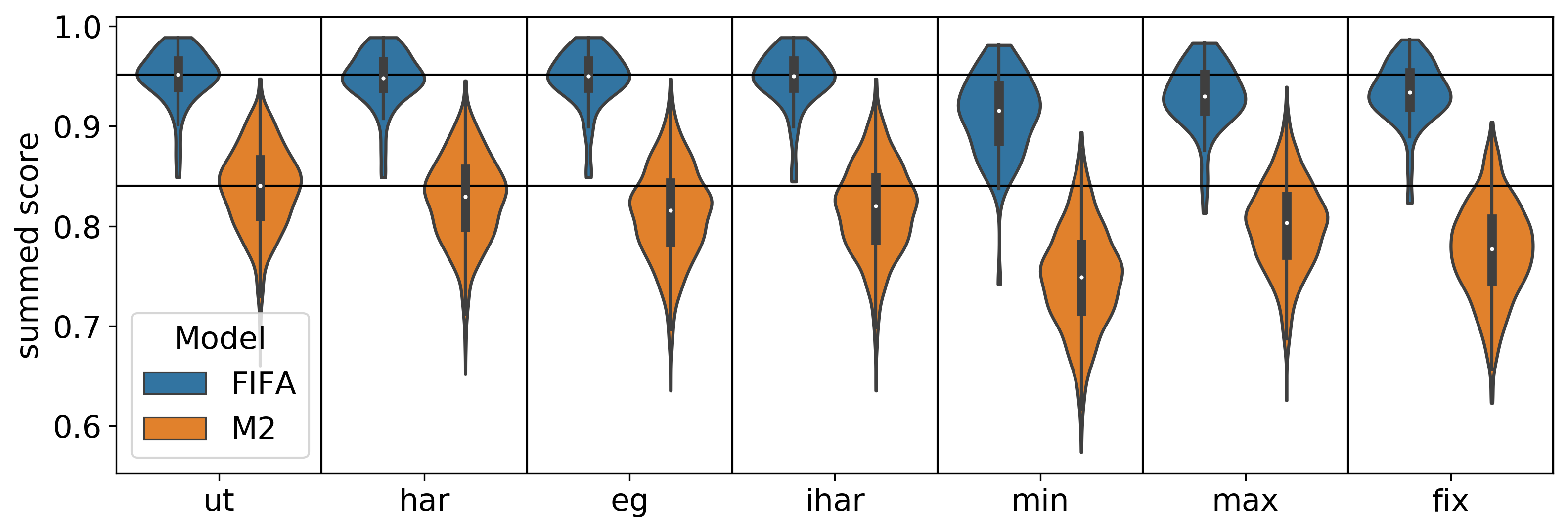
Figure 1: Summed score of winning line-ups for different voting rules. The black horizontal lines indicate the median for the utilitarian rule on the two datasets.

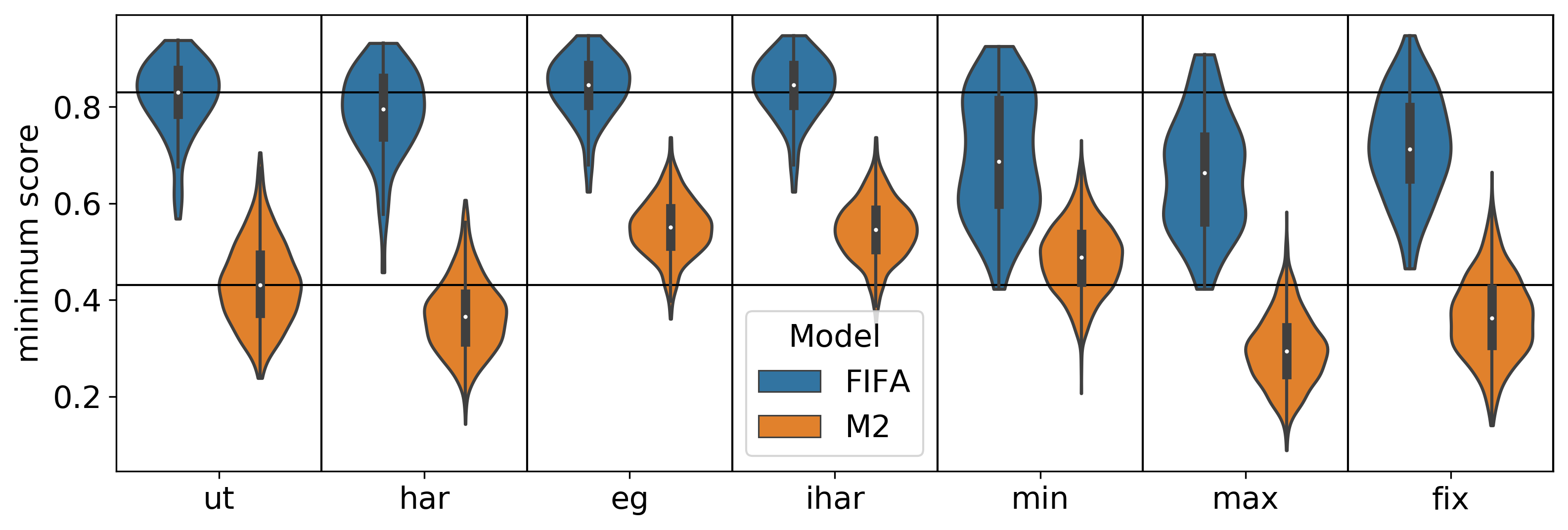
Figure 2: Minimum score in winning line-ups for different voting rules.

Comparison of voting rules. We compare the different voting rules by examining the following four metrics: (i) the summed score of the computed winning line-up $\pi$ normalized by the summed score of the utopic outcome, (ii) the minimum score of a position in the winning line-up, (iii) the Gini coefficient. of the score vector, and (iv) the amount of reasonable dissatisfaction measured as the sum of all reasonable dissatisfactions, that is, the difference between the score of a position $p$ in $\pi$ and the score of a better candidate $c$ on $p$ if the candidate-position pair $(p,c)$ is reasonably dissatisfied. For the egalitarian rule, if multiple line-ups are winning, then we always select the line-up with the highest summed score.

Concerning the summed score (see Figure 1), as expected, all four OWA-rules clearly outperform the three sequential rules. The OWA-rules all behave remarkably similar, especially on the FIFA data. The utilitarian rule produces by definition line-ups with the highest possible summed score, closely followed by the harmonic rule. Turning to the sequential rules, the min-first rule produces the worst results, while the max-first rule produces the best results.

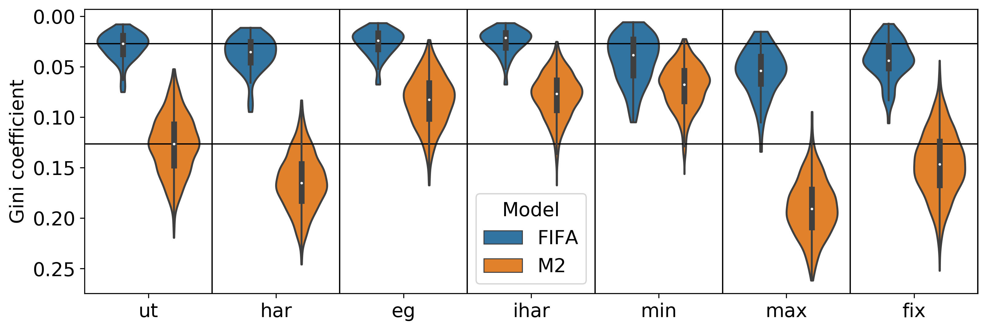
Figure 3: Gini coefficient of score vector of line-ups for different voting rules.

Turning to the minimum score (see Figure 2), the OWA-rules mostly outperform the sequential rules. The two rules with the highest minimum score are the egalitarian rule and the inverse harmonic rule. The utilitarian and harmonic rule produce slightly worse results on the easier FIFA data and significantly worse results on the more demanding M2 data. Among the sequential rules, the min-first rule performs best, sometimes even outperforming the utilitarian rule, while the max-first rule produces the worst results. For the Gini coefficient (see Figure 3), the overall picture is quite similar, i.e., rules that produce line-ups with a higher minimum score also produce line-ups that are more balanced in general.

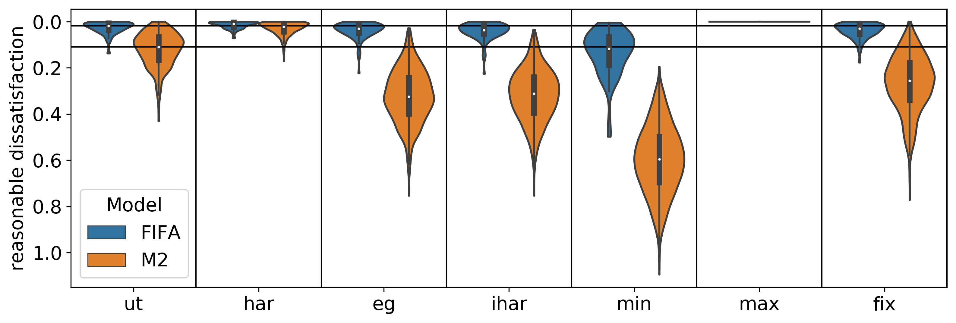
Figure 4: Reasonable dissatisfaction in winning line-ups for different voting rules.

Lastly, considering the amount of reasonable dissatisfaction (see Figure 4), by definition, the max-first rule does not produce any reasonable dissatisfaction. Among the other rules, the harmonic rule produces the best results followed by the utilitarian rule. The egalitarian, inverse harmonic, and fixed-order rule all produce around double the amount of reasonable dissatisfaction, while the min-first rule produces significantly worse results by an additional factor of two.

Summary. Somewhat surprisingly, all OWA-rules outperform all sequential rules for all quantities, with only two exceptions: The min-first rule produces pretty balanced outcomes and the max-first rule produces no reasonable dissatisfaction. However, even if one aims at optimizing mainly one of these two quantities, it is usually recommendable to use an OWA-rule. Selecting the inverse harmonic rule instead of the min-first rule results in outcomes which are comparably balanced, have significantly higher summed and minimum scores, and have way less reasonable dissatisfaction. Using the harmonic rule instead of the max-first rule will introduce only little reasonable dissatisfaction in exchange for more balanced line-ups with higher summed and minimum scores. Comparing the different OWA-rules to each other, it is possible to differentiate the utilitarian and harmonic rule on the one side, from the egalitarian and inverse harmonic rule (which behave particularly similarly) on the other side: Rules from the former class tend to favor more imbalanced line-ups with lower minimum but higher summed score and less reasonable dissatisfaction.

7 Discussion

Overall, the considered OWA-rules produce better outcomes than the sequential rules. Nevertheless, sequential rules might sometimes be at an advantage, since sequential rules are, generally speaking, more transparent, more intuitive, and easier to explain. If one requires a sequential rule, either the fixed-order rule or the max-first rule should be chosen, as the min-first rule violates nearly all studied axioms and produces undesirable outcomes. Focusing on OWA-rules, the harmonic and inverse harmonic rules are rather to be avoided, as they fail to fulfill all considered voting and fairness axioms. Comparing the utilitarian and egalitarian rule, from an axiomatic perspective, the utilitarian rule is at an advantage, because it satisfies the most axioms among all considered rules. However, choosing between these two rules in practice should depend on the application, as the line-ups produced by these rules maximize different metrics. A rule that could somehow incorporate egalitarian and utilitarian considerations is the product rule, which selects outcomes with the highest product of scores.

For future work, it would be interesting to look at line-up elections that take as input the preferences of voters instead of aggregated scores. Analogously to multi-winner voting, new rules for this setting could, for example, focus on selecting proportional and diverse, instead of individually-excellent, line-ups. Such a path would also require developing appropriate axioms. Another possible line of future research could be to run experiments using preference data to examine the influence of the selected single-winner voting rule to aggregate the preferences into scores on the selected line-up. There are also several algorithmic problems that arise from our work. For instance, the computational complexity of computing a winning outcome under the (inverse) harmonic rule and even more generally of computing winning outcomes for arbitrary non-increasing OWA-rules is open.

Appendix A Axiomatic Analysis

A.1 Reasonable Dissatisfaction

Recall that it is possible to model the following situation as a line-up election: A company wants to fill different positions in different teams of the company and publishes an open call for applications to which several candidates respond. The task is then to assign the candidates to the positions in the company. In such a setting, each group offering a job wants to get the best candidate for the job and is unsatisfied if this is not the case. Similarly, each candidate wants to be assigned to the position she is most suitable for. The reasoning behind this is that presumably every candidate prefers to do tasks for which she is qualified and wants to make most out of herself. Unfortunately, line-ups which assign all candidates to their best position and each position its best candidate may not exist. That is why it is necessary to differentiate between different types of dissatisfaction. For example, the dissatisfaction of a candidate who is way less suitable for all positions than all other candidates is hard to circumvent. In contrast, imagine there exists a candidate $c$ who is unsatisfied, as she is either not assigned or assigned to a position for which she is less qualified than for another position $p$ for which, even more, she is more suitable than the current candidate filling $p$. Then, the dissatisfaction of $c$ and the dissatisfaction of $p$ are quite reasonable and voters might agree that assigning $c$ to her current position treated her and position $p$ unfairly. This setup shall motivate and illustrate our definition of reasonable dissatisfaction presented in the main body of the paper. Interestingly, every winning line-up under the max-first rule is reasonable satisfying, which proves the following proposition.

Proposition 3.

In every line-up election, an outcome without reasonable dissatisfaction is guaranteed to exist.

Proof.

Let $E$ be a line-up election. We claim that all winning line-ups $\pi$ of $E$ under the max-first rule are reasonably satisfying, which proves the proposition. Assume that there exist two positions $p$ and $p^{\prime}$ fulfilling the first condition for reasonable dissatisfaction. Then, if $p$ has been filled by the rule before $p^{\prime}$, then it needs to hold that $\operatorname{score}_{p}(\pi_{p})\geq\operatorname{score}_{p}(\pi_{p^{\prime}})$, thereby contradicting the condition. If $p^{\prime}$ were filled by the algorithm before $p$, then it would need to hold that $\operatorname{score}_{p^{\prime}}(\pi_{p^{\prime}})\geq\operatorname{score}_{p}(\pi_{p^{\prime}})$, thereby contradicting the condition. No candidate $c\notin\pi$ and position $p$ can fulfill the second condition of reasonable satisfaction, as otherwise $c$ would have been assigned to $p$. ∎

A.2 Intuitive Explanations of Axioms

In the following, we try to give a more intuitive understanding of the considered axioms by interpreting them in the language of our introductory soccer example. Here, the candidates are the players of the team and positions are positions in a soccer formation. Scores of candidate-positions pairs are derived from approvals of the coaching staff. For all axioms, we present a plausible drawback that might occur if this axiom is violated.

Non-wastefulness

After agreeing on a line-up, the coaches realize that there exists a position and an unassigned player such that the coaches agree that he is more suitable to fill this position than the currently assigned player.

Score Pareto optimality

After agreeing on a line-up, the coaches realize that there exists a different line-up where the coaches agree that, taking all positions into account, this line-up is better than the one which they decided for.

Score consistency

The team of defensive coaches meets and agrees on a line-up. At the same time, the team of offensive coaches meets and agrees independently on the same line-up. Afterwards, all coaches meet together and agree on a line-up that is different from the one that each set of coaches came up with independently.

Position consistency

The defensive coaches agree on a line-up of defenders and midfielders. The offensive coaches agree on a line-up of strikers and midfielders. Both line-ups coincide on the midfielders and no player who is placed as a defender in the first line-up is placed as a striker in the second line-up. However, in a joint meeting, the coaches decide on a full line-up that is different from the line-up of the defensive coaches on the defenders or midfielders (despite the fact that it would have been possible to combine the two initial line-ups).

Monotonicity

The coaches agree on a line-up for a game. In this game, the center-forward plays very well, so afterwards more coaches believe that he is suitable to fill this position. All other opinions remain unchanged. In the next game, some other line-up is chosen.

Line-up enlargement monotonicity

In a training session on a smaller field, the coaches select their best line-up consisting out of five players. The day later, for the next normal game with eleven players, one of these players is benched.

Reasonable satisfaction

The team has a star player where everyone agrees that he is a perfect center-forward and better than everyone else on this position. In the current line-up, he is placed in the midfield and very unsatisfied and demotivated by this.

A.3 Missing Proofs

In the following, we provide for all considered rules and axioms proofs whether the rule satisfies the axiom strongly, weakly, or not at all. We split these proofs into two parts: We start by examining the OWA-rules, before we turn to sequential rules. Moreover, within each section, because often similar ideas are required, we group the results by the axioms. For each axiom, the proofs for the different rules from the considered class can be found next to each other. For an overview of the results, we refer to Table 1 from the main body of the paper. We present the different axioms in the same order as they appear in Table 1.

A.3.1 OWA-rules

We only consider non-negative normalized OWA-vectors $\Lambda$, that is, vectors in which all entries are non-negative and the largest entry is one. It is easily possible to normalize arbitrary OWA-vectors by dividing all entries by the maximum entry in the vector. To explain how we will reason about OWA-rules in the following, let us look at the following line-up election:

	$p_{1}$	$p_{2}$	$p_{3}$
$a$	$1$	$0$	$8$
$b$	$2$	$4$	$5$
$c$	$0$	$6$	$7$

Consider the line-up $(a,b,c)$. It consists of one candidate-position pair with score $1$, namely $a$ who is assigned to $p_{1}$, one candidate-position pair with score $4$, namely $b$ who is assigned to $p_{2}$, and one candidate-position pair of score $7$ namely, $c$ who is assigned to $p_{3}$. Now, imagine that we want to compute the score assigned to this outcome by the harmonic rule, that is, $f^{\Lambda^{\operatorname{har}}}$ with $\Lambda^{\operatorname{har}}=(1,\frac{1}{2},\frac{1}{3})$. The score is the sum of the highest score of a candidate-position pair plus $\frac{1}{2}$ times the second highest score of a candidate-position pair plus $\frac{1}{3}$ times the lowest score of a candidate-position pair. So for the line-up $(a,b,c)$ it is $7+\frac{1}{2}*4+\frac{1}{3}*1=11\frac{1}{3}$. We denote the score of $(a,b,c)$ under the harmonic rule as $\Lambda^{\operatorname{har}}(a,b,c)=\frac{1}{3}*1+\frac{1}{2}*4+7$. Note that we sort the terms of the sum by the ordering of the candidates in the line-up. For instance, the score of the line-up $(b,a,c)$ under the harmonic rule is $\Lambda^{\operatorname{har}}(b,a,c)=\frac{1}{2}*2+\frac{1}{3}*0+1*7.$ We start by examining non-wastefulness.

Theorem 1.

All OWA-rules $f^{\Lambda}$ are weakly non-wasteful and weakly score Pareto optimal. For an OWA vector $\Lambda$ with only strictly positive entries, $f^{\Lambda}$ is strongly non-wasteful and score Pareto optimal.

Proof.

First of all, note that weak score Pareto optimality implies weak non-wastefulness. To prove that all OWA-rules $f^{\Lambda}$ are weakly score Pareto optimal, for the sake of contradiction, let us assume that $f^{\Lambda}$ has returned only score Pareto dominated line-ups. Let $\pi$ be one of these line-ups, which is score Pareto dominated by some line-up $\pi^{\prime}$. However, this implies that $\Lambda(\pi^{\prime})\geq\Lambda(\pi)$, meaning that $\pi^{\prime}$ is also selected as a winning line-up.

Note that for all $\Lambda$ with strictly positive entries, it even holds that $\Lambda(\pi^{\prime})>\Lambda(\pi)$ and thereby that only score Pareto optimal line-ups are selected. However, for OWA-vectors $\Lambda$ with a zero entry at position $i$, $f^{\Lambda}$ is not strongly score Pareto optimal. To see this, consider an election where all scores are different natural numbers. Let $\pi$ be a line-up in which some position $p\in P$ has the $i$-th highest score. However, then the outcome $\pi^{\prime}$ in which each position except $p$ gets assigned the same candidate and $p$ gets assigned a candidate $c$ with $\operatorname{score}_{p}(c)=\operatorname{score}_{p}(\pi)-1$ is still a winning line-up but obviously score Pareto dominated by $\pi^{\prime}$.

The same arguments can also be used to prove the statement for non-wastefulness. ∎

Theorem 2.

For all OWA-vectors $\Lambda\neq(1,0,\dots,0)$, $f^{\Lambda}$ is not weakly reasonable satisfying. For $\Lambda=(1,0,\dots,0)$, $f^{\Lambda}$ is weakly but not strongly reasonably satisfying.

Proof.

Here and in some of the following proofs, we prove the two negative parts only for OWA-vectors of size two. However, it is easily possible to generalize the provided counterexamples to arbitrary OWAs of size $k>2$ by inserting $k-2$ positions and, for each position, a designated candidate. For each inserted position, all candidates except the designated candidate have a high negative score, while the designated candidate has a score which is either above every score used in the example or slightly below every score used in the example. By selecting how many of the $k-2$ designated candidates have a score above or below the scores from the example, it is possible to select the window in the OWA-vector the example accounts for.

Let us consider the following two-candidates two-positions line-up election. Let $\Lambda$ be an arbitrary length-two OWA-vector without zero entries and let $0<x<1$ be the smaller of the two entries of $\Lambda$ (i.e., we have either $\Lambda=(1,x)$ or $\Lambda=(x,1)$; we will treat the two cases $(1,0)$ and $(0,1)$ separately). Let us consider the following line-up election:

	$p_{1}$	$p_{2}$
$a$	$1$	$1+\frac{y}{2}$
$b$	$0$	$1$

with $y=x$. In this election, outcome $(a,b)$ has score $1+x$ under OWA-vector $\Lambda$, while outcome $(b,a)$ depending on whether $\Lambda$ is decreasing or increasing has score either  $1+\frac{x}{2}$ or $x+\frac{x\cdot x}{2}$. Consequently, $(a,b)$ is selected as the unique winner by all $f^{\Lambda}$ with $\Lambda\neq(1,0)$ and $\Lambda\neq(0,1)$. However, in the outcome $(a,b)$, the candidate-position pair $(a,p_{2})$ is reasonably dissatisfied, as $a$’s score for position $p_{2}$ is higher than $b$’s score for position $p_{2}$ and higher than $a$’s score for position $p_{1}$.

For $\Lambda=(0,1)$, we can use the election from above with arbitrary strictly positive $y$. In any case, $f^{\Lambda}$ will select $(a,b)$ as the unique winning line-up. In this line up, the candidate-position pair $(a,p_{2})$ is reasonably dissatisfied.

To prove that $f^{(1,0,\dots)}$ is weakly reasonable satisfying, let $\pi$ be a winning line-up of some line-up election under $f^{(1,0,\dots)}$. Let $(c,p)$ be the candidate-position pair with the highest score in $\pi$. It follows that this is the highest score $c$ can achieve and the highest score $p$ can achieve, as otherwise $\pi$ would not be a winning line-up. Moreover, all line-ups $\pi^{\prime}$ with $\pi_{p}=\pi^{\prime}_{p}$ are also winning line-ups. One of them is guaranteed to be reasonable satisfying, as all line-ups provided by the max-first rule are included in them. Clearly, due to the zero entries, one can easily construct examples where some of these winning line-ups cause reasonable dissatisfaction. ∎

Theorem 3.

For all OWA-vectors $\Lambda\neq(1,\dots 1)$, $f^{\Lambda}$ is not weakly score consistent. The utilitarian rule, $f^{\operatorname{ut}}$, is strongly score consistent.

Proof.

To prove the first part, let us consider the following two-candidates two-positions line-up election that can be extended to an arbitrary number of candidates and positions:

$E$: $p_{1}$ $p_{2}$ $a$ 4 3 $b$ 2 1   $E^{\prime}$: $p_{1}$ $p_{2}$ $a$ 1 3 $b$ 2 4   $E^{*}$: $p_{1}$ $p_{2}$ $a$ 5 6 $b$ 4 5

For $f^{(1,x)}$ with $x\in[0,1)$, in the first election $E$, it holds that $\Lambda(a,b)=4+x>2x+3=\Lambda(b,a)$. In the second election, it holds that $\Lambda(a,b)=x+4>2x+3=\Lambda(b,a)$. However, in the combined election $E^{*}$, where we summed up the score matrices of the first two elections, it holds that $\Lambda(a,b)=5+5x<4x+6=\Lambda(b,a)$. Hence, weak score consistency is violated.

For $f^{(x,1)}$ with $x\in[0,1)$, in the first election, it holds that $\Lambda(a,b)=4x+1<2+3x=\Lambda(b,a)$ in the first election. In the second election, it holds that $\Lambda(a,b)=1+4x<2+3x=\Lambda(b,a)$. However, in the combined election $E^{*}$, where we summed up the score matrices of the first two elections, it holds that $\Lambda(a,b)=5x+5>4+6x=\Lambda(b,a)$, which violates score consistency.

It remains to prove that $f^{\operatorname{ut}}$ is strongly score consistent. Let $\pi$ be some winning line-up in the two original elections $E=(\mathbf{S},C,P)$ and $E^{\prime}=(\mathbf{S}^{\prime},C,P)$. We show that $\pi$ is a winner in $E^{*}$. For the sake of contradiction, let us assume that there exists a line-up $\pi^{\prime}$ with a higher utilitarian score than $\pi$ in the combined election $E^{*}=(\mathbf{S}+\mathbf{S}^{\prime},C,P)$. However, as it holds that the score of a line-up in $E^{*}$ is equal to the sum of the scores of this line-up in $E$ and $E^{\prime}$, this implies that for at least one of the two initial elections it also needs to hold that the score of $\pi^{\prime}$ is higher than the score of $\pi$. However, this contradicts the assumption that $\pi$ is a winning line-up for both $E$ and $E^{\prime}$.

To prove that the utilitarian rule also satisfies condition (b) of score consistency, let $\pi$ be some winning line-up $\pi$ of the combined election $E^{*}$ that is also a winning line-up in both $E$ and $E^{\prime}$ (such $\pi$ must exist due to the above argument for the first direction). Let $\Lambda^{\operatorname{ut}}_{E}(y)$ denote the utilitarian score of a line-up $y$ in an election $E$. Let $\pi^{\prime}\neq\pi$ be another line-up that is also winning in the combined election (if such a line-up exists). We show that $\pi^{\prime}$ is a winner in $E$ and $E^{*}$ as well. Since both $\pi^{\prime}$ and $\pi$ win in $E^{*}$, it holds that $\Lambda^{\operatorname{ut}}_{E^{*}}(\pi)=\Lambda^{\operatorname{ut}}_{E^{*}}(\pi^{\prime})$. Moreover, as $\pi$ wins in $E$ and $E^{\prime}$, $\Lambda^{\operatorname{ut}}_{E}(\pi)\geq\Lambda^{\operatorname{ut}}_{E}(\pi^{\prime})$ and $\Lambda^{\operatorname{ut}}_{E^{\prime}}(\pi)\geq\Lambda^{\operatorname{ut}}_{E^{\prime}}(\pi^{\prime})$. For every line-up $x$, we have that $\Lambda^{\operatorname{ut}}_{E^{*}}(x)=\Lambda^{\operatorname{ut}}_{E}(x)+\Lambda^{\operatorname{ut}}_{E^{\prime}}(x)$, which implies that $\Lambda^{\operatorname{ut}}_{E}(\pi)=\Lambda^{\operatorname{ut}}_{E}(\pi^{\prime})$ and $\Lambda^{\operatorname{ut}}_{E^{\prime}}(\pi)=\Lambda^{\operatorname{ut}}_{E^{\prime}}(\pi^{\prime})$. Hence, $\pi^{\prime}$ is a winning line-up in $E$ and $E^{\prime}$. ∎

Theorem 4.

The harmonic rule, $f^{\operatorname{har}}$, and the inverse harmonic rule, $f^{\operatorname{ihar}}$, violate weak position consistency. The egalitarian rule, $f^{\operatorname{eg}}$, and the utilitarian rule, $f^{\operatorname{ut}}$, are weak but not strong position consistent.

Proof.

Harmonic rule $f^{\operatorname{har}}$: Let $P^{\prime}=\{p_{1},p_{2}\}$ and $P^{\prime\prime}=\{p_{2},p_{3}\}$ and let $E^{*}=(\mathbf{S},C,P^{\prime}\cup P^{\prime\prime})$ be the following line-up election:

	$p_{1}$	$p_{2}$	$p_{3}$
$a$	$1$	$3$	$0$
$b$	$3$	$4.1$	$0$
$c$	$0$	$0$	$5$

In the first sub-election, $E^{\prime}=(\mathbf{S},C,P^{\prime})$, it holds that $\Lambda^{\operatorname{har}}(a,b)=\frac{1}{2}\cdot 1+1\cdot 4.1>1\cdot 3+\frac{1}{2}\cdot 3=\Lambda^{\operatorname{har}}(b,a)$. Thus, $(a,b)$ is the unique winning line-up. In the second sub-election, $E^{\prime\prime}=(\mathbf{S},C,P^{\prime\prime})$, $(b,c)$ is the unique winning line-up. However, in the full election $E^{*}$, $\Lambda^{\operatorname{har}}(a,b,c)=\frac{1}{3}\cdot 1+\frac{1}{2}\cdot 4.1+1\cdot 5<\frac{1}{2}\cdot 3+\frac{1}{3}\cdot 3+1\cdot 5=\Lambda^{\operatorname{har}}(b,a,c)$. Thereby, $(a,b,c)$ is not a winning line-up, which violates weak position consistency.

Inverse harmonic rule $f^{\operatorname{ihar}}$: Let $P^{\prime}=\{p_{1},p_{2}\}$ and $P^{\prime\prime}=\{p_{2},p_{3}\}$ and let $E^{*}=(\mathbf{S},C,P^{\prime}\cup P^{\prime\prime})$ be the following line-up election:

	$p_{1}$	$p_{2}$	$p_{3}$
$a$	$2$	$1$	$0$
$b$	$3\frac{3}{4}$	$2$	$0$
$c$	$0$	$0$	$\frac{1}{2}$

In the first sub-election, $E^{\prime}=(\mathbf{S},C,P^{\prime})$, $(a,b)$ is the unique winning line-up, as $\Lambda^{\operatorname{ihar}}(a,b)=\frac{1}{2}\cdot 2+1\cdot 2>\frac{1}{2}\cdot 3\frac{3}{4}+1\cdot 1=\Lambda^{\operatorname{ihar}}(b,a)$. In the second sub-election, $E^{\prime\prime}=(\mathbf{S},C,P^{\prime\prime})$, $(b,c)$ is the unique winning line-up. However, in the full election $E^{*}$, $\Lambda^{\operatorname{ihar}}(a,b,c)=\frac{1}{3}\cdot 2+\frac{1}{2}\cdot 2+1\cdot\frac{1}{2}<\frac{1}{3}\cdot 3\frac{3}{4}+\frac{1}{2}\cdot 1+1\cdot\frac{1}{2}=\Lambda^{\operatorname{ihar}}(b,a,c)$. Thereby, $(a,b,c)$ is not a winning line-up, which violates weak position consistency.

Egalitarian rule $f^{\operatorname{eg}}$: We start by proving that this rule satisfies weak position consistency. Assume that $E^{*}=(\mathbf{S},C,P)$ is a line-up election and $P^{\prime},P^{\prime\prime}\subseteq P$ with $P^{\prime}\cup P^{\prime\prime}=P$. Let $\pi^{\prime}$ be a winning line-up of the election $E^{\prime}=(\mathbf{S},C,P^{\prime})$ and $\pi^{\prime\prime}$ be a winning line-up of the election $E^{\prime\prime}=(\mathbf{S},C,P^{\prime\prime})$, where $\pi^{\prime}$ and $\pi^{\prime\prime}$ are overlapping-disjoint. We claim that $\pi^{\prime}\cup\pi^{\prime\prime}$ is then a winning line-up of the full election $E^{*}$. First of all, note that for all outcomes $\pi^{*}$ of the full election $E^{*}$ it holds that $\min(\Lambda^{\operatorname{eg}}(\pi^{*}|_{P}),\Lambda^{\operatorname{eg}}(\pi^{*}|_{P^{\prime}}))=\Lambda^{\operatorname{eg}}(\pi^{*})$. Thereby, the existence of an outcome of the combined election $\pi^{*}$ with higher score than $\pi^{\prime}\cup\pi^{\prime\prime}$ implies that either $\Lambda^{\operatorname{eg}}(\pi^{*}|_{P^{\prime}})>\Lambda^{\operatorname{eg}}(\pi^{\prime})$, which contradicts the assumption that $\pi^{\prime}$ is a winning line-up of $E^{\prime}$, or $\Lambda^{\operatorname{eg}}(\pi^{*}|_{P^{\prime\prime}})>\Lambda^{\operatorname{eg}}(\pi^{\prime\prime})$, which contradicts the assumption that $\pi^{\prime\prime}$ is a winning line-up of $E^{\prime\prime}$.

To prove that $f^{\operatorname{eg}}$ does not satisfy strong position consistency, we exploit the property that not all winning line-ups are score Pareto optimal. Consider the following line-up election $E^{*}=(\mathbf{S},C,P)$:

	$p_{1}$	$p_{2}$	$p_{3}$
$a$	$1$	$0$	$0$
$b$	$0$	$3$	$2$
$c$	$0$	$2$	$3$

In the sub-election on $P^{\prime}=\{p_{1},p_{2}\}$, $(a,b)$ is the unique winning line-up. On $P^{\prime\prime}=\{p_{2},p_{3}\}$, $(b,c)$ is the unique winning line-up. However, in the full election, $(a,c,b)$ is also a winning line-up, which violates strong position consistency.

Utilitarian rule $f^{\operatorname{ut}}$: We prove that $f^{\operatorname{ut}}$ satisfies weak but not strong position consistency. Let again $E^{*}=(\mathbf{S},C,P)$ be a line-up elections and $P^{\prime},P^{\prime\prime}\subseteq P$ with $P^{\prime}\cup P^{\prime\prime}=P$. In the following, we write $L$ to denote $P^{\prime}\setminus P^{\prime\prime}$, $M$ to denote $P^{\prime}\cap P^{\prime\prime}$ and $R$ to denote $P^{\prime\prime}\setminus P^{\prime}$.

Assume that $\pi^{\prime}$ is a winning line-up of the first sub-election $E^{\prime}=(\mathbf{S},C,P^{\prime})$ on $P^{\prime}$ and $\pi^{\prime\prime}$ of the second sub-election $E^{\prime\prime}=(\mathbf{S},C,P^{\prime\prime})$ on $P^{\prime\prime}$, where $\pi^{\prime}$ and $\pi^{\prime\prime}$ are overlapping-disjoint. We claim that $\pi^{*}=\pi^{\prime}\cup\pi^{\prime\prime}$ is then a winning line-up of the full election $E^{*}$.

Assume, for the sake of contradiction, that there exists a line-up $\widetilde{\pi}^{*}$ of $E^{*}$ with a higher utilitarian score than $\pi^{*}$. Let $\widetilde{\pi}^{\prime}:=\widetilde{\pi}^{*}|_{P^{\prime}}$ and $\widetilde{\pi}^{\prime\prime}:=\widetilde{\pi}^{*}|_{P^{\prime\prime}}$. As $\pi^{\prime}$ and $\pi^{\prime\prime}$ are winning line-ups, it needs to hold that $\Lambda^{\operatorname{ut}}(\pi^{\prime})\geq\Lambda^{\operatorname{ut}}(\widetilde{\pi}^{\prime})$ and $\Lambda^{\operatorname{ut}}(\pi^{\prime\prime})\geq\Lambda^{\operatorname{ut}}(\widetilde{\pi}^{\prime\prime})$. From this it follows that

$$\Lambda^{\operatorname{ut}}(\widetilde{\pi}^{*}|_{L})+\Lambda^{\operatorname{ut}}(\widetilde{\pi}^{*}|_{M})\leq\Lambda^{\operatorname{ut}}(\pi^{*}|_{L})+\Lambda^{\operatorname{ut}}(\pi^{*}|_{M})\text{ and }$$

$$\Lambda^{\operatorname{ut}}(\widetilde{\pi}^{*}|_{M})+\Lambda^{\operatorname{ut}}(\widetilde{\pi}^{*}|_{R})\leq\Lambda^{\operatorname{ut}}(\pi^{*}|_{M})+\Lambda^{\operatorname{ut}}(\pi^{*}|_{R}).$$

Hence,

$$\Lambda^{\operatorname{ut}}(\widetilde{\pi}^{*}|_{L})+2\cdot\Lambda^{\operatorname{ut}}(\widetilde{\pi}^{*}|_{M})+\Lambda^{\operatorname{ut}}(\widetilde{\pi}^{*}|_{R})\leq\Lambda^{\operatorname{ut}}(\pi^{*}|_{L})+2\cdot\Lambda^{\operatorname{ut}}(\pi^{*}|_{M})+\Lambda^{\operatorname{ut}}(\pi^{*}|_{R})$$ (1)

Recall that, assuming that $\widetilde{\pi}^{*}$ has a higher score than $\widetilde{\pi}$, it needs to hold that:

$$\Lambda^{\operatorname{ut}}(\widetilde{\pi}^{*})= \Lambda^{\operatorname{ut}}(\widetilde{\pi}^{*}|_{L})+\Lambda^{\operatorname{ut}}(\widetilde{\pi}^{*}|_{M})+\Lambda^{\operatorname{ut}}(\widetilde{\pi}^{*}|_{R})>$$ (2)

$$\Lambda^{\operatorname{ut}}(\pi^{*}|_{L})+\Lambda^{\operatorname{ut}}(\pi^{*}|_{M})+\Lambda^{\operatorname{ut}}(\pi^{*}|_{R})=\Lambda^{\operatorname{ut}}(\pi^{*}).$$

The only possibility that both inequality (1) and (2) hold at the same time is that $\Lambda^{\operatorname{ut}}(\pi^{*}|_{M})-\Lambda^{\operatorname{ut}}(\widetilde{\pi}^{*}|_{M})=x$ and $\Lambda^{\operatorname{ut}}(\widetilde{\pi}^{*}|_{L})-\Lambda^{\operatorname{ut}}(\pi^{*}|_{L})=y$ and $\Lambda^{\operatorname{ut}}(\widetilde{\pi}^{*}|_{R})-\Lambda^{\operatorname{ut}}(\pi^{*}|_{R})=y$ for some $x,y,z>0$ with $x<y+z$.

For the sake of contradiction, assume that an outcome $\widetilde{\pi}^{*}$ that fulfills the thee conditions specified above exists. We now compare $\pi^{*}$ and $\widetilde{\pi}^{*}$ and argue why this is not possible. Let us first look at the differences of $\pi^{*}$ and $\widetilde{\pi}^{*}$ on $L$: Because of the optimality of $\pi^{\prime}$, it is not possible to increase the score of $\pi^{*}$ on $L$ by using candidates who are not already assigned in $\pi^{*}$ to positions from $M$. Thereby, in $\widetilde{\pi}^{*}|_{L}$ some candidates from $\pi^{*}|_{L}$ must have been replaced by some candidates from $\pi^{*}|_{M}$. From the optimality of $\pi^{\prime}$ it follows that by modifying $L$ as described above, an increase of $\Lambda^{\operatorname{ut}}(\pi^{*}|_{L})$ by some $x$ always results in a decrease of at least $x$ on $\Lambda^{\operatorname{ut}}(\pi^{*}|_{M})$. Moreover, it is never possible to increase the score on $R$ simultaneously by such rearrangements, as all candidates that might get free are candidates from $R$ which are—due to the optimality of $\pi^{\prime\prime}$— not usable to increase the score on $L$. As the same argument also holds for $R$, it is never possible to increase the scores as required and thereby $\pi^{*}$ is always a winning line-up.

We consider the following line-up election $E^{*}=(\mathbf{S},C,P)$ to prove that $f^{\operatorname{ut}}$ violates strong position consistency:

	$p_{1}$	$p_{2}$	$p_{3}$
$a$	$0$	$0$	$0$
$b$	$1$	$1$	$0$
$c$	$0$	$0$	$0$

In the sub-election on $P^{\prime}=\{p_{1},p_{2}\}$, $(a,b)$ is a winning outcome. On $P^{\prime\prime}=\{p_{2},p_{3}\}$, $(b,c)$ is winning outcome. However, in the full election $E^{*}$, $(b,a,c)$ is a winning outcome. However $(a,c)$ is not a winning outcome of the second sub-election on $P^{\prime\prime}$. ∎

Theorem 5.

The utilitarian rule, $f^{\operatorname{ut}}$, satisfies strong monotonicity. The egalitarian rule, $f^{\operatorname{eg}}$, violates weak monotonicity. For all OWA-vectors $\Lambda$ with at least three succeeding non-zero entries of which the last two are unequal, $f^{\Lambda}$ does not satisfy weak monotonicity.

Proof.

Utilitarian rule $f^{\operatorname{ut}}$: We show that $f^{\operatorname{ut}}$ satisfies strong monotonicity. Let $\pi$ be a winning line-up of some line-up election $(\mathbf{S},C,P)$. Then, by increasing $\operatorname{score}_{p}(c)$ for some $(c,p)\in C\times P$ with $c=\pi_{p}$ by some arbitrary $x$, the score of $\pi$ is increased by $x$. Moreover, the score of all other line-ups is also increased by at most $x$. Thereby, $\pi$ remains a winning line-up, and no new winning line-ups can be created, as every line-up that is winning in the modified elections needs to have the same utilitarian score as $\pi$ before the modification.

Egalitarian rule $f^{\operatorname{eg}}$: Consider the following line-up election:

	$p_{1}$	$p_{2}$
$a$	$0$	$3$
$b$	$3$	$0$
$c$	$4$	$0$

Under the egalitarian rule, $(b,a)$ is a winning line-up of this election. However, after increasing the score of $a$ on $p_{2}$ to four, $(b,a)$ is no longer a winning line-up, as now $(c,a)$ is the unique winning line-up.

(Inverse) harmonic rule $f^{\operatorname{har}}$/$f^{\operatorname{ihar}}$: Finally, we prove that for all OWA-vectors $\Lambda$ with at least three succeeding non-zero entries of which the last two are not equal, $f^{\Lambda}$ does not satisfy weak monotonicity. Note that this also includes the harmonic rule and inverse harmonic rule. Let $\Lambda=(x,y,z)$. We assume that $x\neq 0$ and $y\neq z$. Consider the following line-up election:

	$p_{1}$	$p_{2}$	$p_{3}$
$a$	$4$	$1$	$0$
$b$	$4+\frac{0.5y+1.5z}{x}$	$3$	$0$
$c$	$0$	$0$	$2$

Clearly, in all winning line-ups, $c$ is assigned to $p_{3}$. Thereby, the two line-ups which could be winning are $(a,b,c)$ and $(b,a,c)$ with scores $\Lambda(a,b,c)=4x+3y+2z$ and $\Lambda(b,a,c)=x\cdot(4+\frac{0.5y+1.5z}{x})+1z+2y=4x+2.5y+2.5z$. We now increase $\operatorname{score}_{p_{3}}(c)$ to $3$. The scores of $(a,b,c)$ and $(b,a,c)$ change as follows: $\Lambda(a,b,c)=4x+3y+3z$ and $\Lambda(b,a,c)=4x+3.5y+2.5z$. Assuming now that $y>z$, $(a,b,c)$ is the unique winning line-up in the original election. However, in the altered election, $(b,a,c)$ is the unique winning line-up. This violates weak monotonicity. Assuming $z>y$, $(b,a,c)$ is the unique winning line-up in the original election, while $(a,b,c)$ is the unique winning line-up in the altered election. This violates weak monotonicity. ∎

Theorem 6.

The egalitarian rule, $f^{\operatorname{eg}}$, satisfies weak line-up enlargement monotonicity but fails to satisfy strong line-up enlargement monotonicity. The utilitarian rule, $f^{\operatorname{ut}}$, satisfies strong line-up enlargement monotonicity. The harmonic rule, $f^{\operatorname{har}}$, and inverse harmonic rule, $f^{\operatorname{ihar}}$, both fail weak line-up enlargement monotonicity.

Proof.

Egalitarian rule $f^{\operatorname{eg}}$: We prove that $f^{\operatorname{eg}}$ satisfies weak line-up enlargement monotonicity. Let $\pi$ be a winning line-up of the initial election $E=(\mathbf{S},C,P)$ of egalitarian score $x$. Let $\pi^{\prime}$ be a winning line-up of the extended election $E^{\prime}=(\mathbf{S}^{\prime},C,P\cup\{p^{*}\})$ such that there exists a candidate $c\in C$ with $c\notin\pi^{\prime}$ and $c\in\pi$. Let $y$ be the egalitarian score of $\pi^{\prime}$. It needs to hold that $x\geq y$, as otherwise $\pi$ cannot be a winning line-up of the initial election. We claim that it is always possible to construct from $\pi^{\prime}$ a winning line-up $\pi^{\prime\prime}$ of the extended election such that $\pi_{P}\subseteq\pi^{\prime\prime}_{P\cup\{p^{*}\}}$. We construct $\pi^{\prime\prime}$ from $\pi$ and $\pi^{\prime}$ using the following iterative procedure. Initially, we set $\pi^{\prime\prime}:=\pi^{\prime}$. As long as there exists a candidate $c\in C$ with $c\in\pi$ and $c\notin\pi^{\prime\prime}$, we set $\pi^{\prime\prime}_{\pi(c)}=c$. As the egalitarian score of $\pi$ is $x$, for all $c\in\pi$, it holds that $\operatorname{score}_{\pi(c)}(c)\geq x$. Thus, the egalitarian score of $\pi^{\prime\prime}$ will not fall below $y$ by the described replacements. Consequently, $\pi^{\prime\prime}$ is a winning line-up of the extended election $E^{\prime}$ with all candidates appearing in $\pi$ also appearing in $\pi^{\prime\prime}$.

However, $f^{\operatorname{eg}}$ fails to satisfy strong line-up enlargement monotonicity. To see this, consider the following line-up election:

	$p_{1}$	$p_{2}$	$p^{*}$
$a$	$3$	$0$	$0$
$b$	$2$	$3$	$0$
$c$	$0$	$2$	$0$
$d$	$0$	$0$	$1$

We consider the election on $p_{1}$ and $p_{2}$ as the initial election. In this initial election, $(a,b)$ is the unique winning line-up. However, as the new position decreases the lowest score in an optimal outcome, $(b,c,d)$ is also a winning line-up in the extended election. Hence, strong line-up-monotonicity is violated.

Utilitarian rule $f^{\operatorname{ut}}$: For a proof that$f^{\operatorname{ut}}$ satisfies weak line-up enlargement monotonicity see Proposition 2.

Using a similar argument as in Proposition 2, we prove that $f^{\operatorname{ut}}$ is even strong line-up enlargement monotone. Let $\pi^{\prime}$ be a winning outcome of the extended election and $\pi$ a winning outcome of the original election where there exists a candidate $c\in C$ that is part of $\pi$ but not of $\pi^{\prime}$, that is, $c\in\pi$ but $c\notin\pi^{\prime}$. To prove that for every winning outcome of the extended election, there always exists a winning outcome of the original election consisting of a subset of candidates of the extended outcome, we construct from $\pi$ an outcome of the original election $\widetilde{\pi}$ with $\widetilde{\pi}|_{P}\subseteq\pi^{\prime}_{P\cup\{p^{*}\}}$ as follows. We start by setting $\widetilde{\pi}:=\pi$. Subsequently, as long as there exists a position $p\in P$ with $\widetilde{\pi}_{p}\notin\pi^{\prime}$ or an unassigned position $p\in P$, we set $\widetilde{\pi}_{p}=\pi^{\prime}_{p}$. If $\pi^{\prime}_{p}$ was already assigned to some other position in $\widetilde{\pi}$, then we delete $\pi^{\prime}_{p}$ from the position she was assigned to in $\widetilde{\pi}$.

It obviously holds that $\widetilde{\pi}\subseteq\pi^{\prime}$. We claim that $\widetilde{\pi}$ is a winning line-up of the initial election. For the sake of contradiction, let us assume that this is not the case, that is, $\Lambda^{\operatorname{ut}}(\widetilde{\pi})<\Lambda^{\operatorname{ut}}(\pi)$. Let $\widetilde{P}\subseteq P$ be the set of positions which have been modified in $\widetilde{\pi}$, where it needs to hold that $\Lambda^{\operatorname{ut}}(\pi^{\prime}|_{\widetilde{P}})<\Lambda^{\operatorname{ut}}(\pi|_{\widetilde{P}})$. Let $\pi^{\prime}_{\textrm{alt}}$ be a line-up resulting from taking $\pi^{\prime}$ and modifying it such that $\pi^{\prime}_{\textrm{alt}}|_{\widetilde{P}}=\pi|_{\widetilde{P}}$. Consequently, $\pi^{\prime}_{\textrm{alt}}$ has a higher utilitarian score than that of $\pi^{\prime}$. It remains to argue that after the modification $\pi^{\prime}_{\textrm{alt}}$ remains a valid line-up, that is, every candidate is assigned at most once in $\pi^{\prime}_{\textrm{alt}}$. To prove this it is enough to show that, for each $p\in\widetilde{P}$, if $\pi_{p}\in\pi^{\prime}$, then $\pi^{\prime}(\pi_{p})\in\widetilde{P}$. Let us fix some position $p\in\widetilde{P}$ such that $\pi_{p}\in\pi^{\prime}$. Note that position $p$ had to be empty at some point during the construction of $\widetilde{\pi}$. This implies that in some preceding step, $\pi_{p}$ had been assigned to some other position in $\widetilde{\pi}$. However, by the construction of $\widetilde{\pi}$, each $c\in\pi^{\prime}$ can be only assigned to position $\pi^{\prime}(c)$ in $\widetilde{\pi}$. Thus, since $\pi_{p}$ must have once been assigned, $\pi_{p}$ was assigned to position $\pi^{\prime}(\pi_{p})$; hence, $\pi^{\prime}(\pi_{p})\in\widetilde{P}$. So $\pi^{\prime}_{\textrm{alt}}$ is indeed a valid line-up.

Harmonic rule $f^{\operatorname{har}}$: To prove that $f^{\operatorname{har}}$ violates weak line-up enlargement monotonicity, consider the following line-up election:

	$p_{1}$	$p_{2}$	$p^{*}$
$a$	$0.5$	$0$	$0$
$b$	$3$	$3.3$	$0$
$c$	$0$	$1$	$0$
$d$	$0$	$0$	$4$

Let the election on $p_{1}$ and $p_{2}$ be the initial election. The underlying idea of the counterexample is that the weighting of the scores may change after adding an additional position. In the initial election, $(a,b)$ is the unique winning line-up as $\Lambda(a,b)=\frac{1}{2}\cdot 0.5+3.3>3+\frac{1}{2}\cdot 1=\Lambda(b,c)$. However, in the full election, $(b,c,d)$ is the unique winning line-up, as $\Lambda(b,c,d)=\frac{1}{2}\cdot 3+\frac{1}{3}\cdot 1+4>\frac{1}{3}\cdot 0.5+\frac{1}{2}\cdot 3.3+4=\Lambda(a,b,d)$.

Inverse harmonic rule $f^{\operatorname{ihar}}$: To prove that $f^{\operatorname{ihar}}$ violates weak line-up enlargement monotonicity, let us consider the following line-up election:

	$p_{1}$	$p_{2}$	$p^{*}$
$a$	$1.7$	$0$	$0$
$b$	$3$	$1.7$	$0$
$c$	$0$	$1$	$0$
$d$	$0$	$0$	$1$

Again, let the election on $p_{1}$ and $p_{2}$ be the initial election. In the initial election, $(a,b)$ is the unique winning line-up as $\Lambda(a,b)=\frac{1}{2}\cdot 1.7+1.7>\frac{1}{2}\cdot 3+1=\Lambda(b,c)$. However, in the full election, $(b,c,d)$ is the unique winning line-up, as $\Lambda(b,c,d)=\frac{1}{3}\cdot 3+\frac{1}{2}\cdot 1+1>\frac{1}{3}\cdot 1.7+\frac{1}{2}\cdot 1.7+1=\Lambda(a,b,d)$. ∎

A.3.2 Sequential rules

We now turn to sequential rules and prove all statements from Table 1. We group again the statements for all three rules by the axioms. Note that for the fixed-order rule, without loss of generality, we assume that the positions in $P=\{p_{1},\dots,p_{q}\}$ are filled in increasing order of their index, that is, $p_{1}$ is filled first, then $p_{2}$ is filled, and so on.

Theorem 7.

All sequential rules satisfy strong non-wastefulness.

Proof.

Assume that $\pi$ is selected as a winning line-up by some sequential rule $f^{\operatorname{seq}}$ and that $\pi$ is wasteful because there exist a $c\notin\pi$ and a position $p\in P$ such that $\operatorname{score}_{p}(c)>\operatorname{score}_{p}(\pi)$. This implies that $c$ would have been selected instead of $\pi_{p}$ to fill position $p$. ∎

Theorem 8.

The fixed-order rule, $f^{\operatorname{seq}}_{\operatorname{fix}}$, and the max-first rule, $f^{\operatorname{seq}}_{\operatorname{max}}$, are weakly but not strongly score Pareto optimal. The min-first rule, $f^{\operatorname{seq}}_{\operatorname{min}}$, fails weak score Pareto optimality.

Proof.

Fixed-order rule $f^{\operatorname{seq}}_{\operatorname{fix}}$: We prove that $f^{\operatorname{seq}}_{\operatorname{fix}}$ is weak score Pareto optimal. Assume that $\pi$ is a winning line-up which is score Pareto dominated by some line-up score Pareto optimal line-up $\pi^{\prime}$. Then, it follows that there exists a winning outcome $\widetilde{\pi}$ that score Pareto dominates $\pi$ on the first $i$ positions for some $i\in[1,k]$: This can be constructed by choosing at every position $p$ the candidate with the maximum score. If ties are present, then choose the candidate $\pi^{\prime}_{p}$ if she is among the candidates with the highest score and otherwise arbitrarily some candidate with the highest score. If, for all positions $p\in P$, $\pi^{\prime}_{p}$ got selected, then we are done, as this implies that the score Pareto optimal line-up $\pi^{\prime}$ is winning under the fixed-order rule. Otherwise, let $p_{i}$ be the first position where $\pi^{\prime}_{p_{i}}$ is not selected, which implies that there exists a candidate with a higher score for $p_{i}$ and that this candidate is selected. Thereby, the score of $\widetilde{\pi}$ is equal to the score of $\pi^{\prime}$ on the first $i-1$ positions and higher than the score of $\pi^{\prime}$ at position $p_{i}$. Now, either $\widetilde{\pi}$ is score Pareto optimal and we are done or there exists again a line-up that score Pareto dominates $\widetilde{\pi}$. If this is again the case, then we can again construct a winning outcome $\widetilde{\pi}^{\prime}$ that score Pareto dominates $\widetilde{\pi}$ on the first $i$ positions for some $i\in[1,k]$. To prove that this process converges to an outcome outputted by the fixed-order rule that is score Pareto optimal, we read the score vector of an outcome $(\operatorname{score}_{p_{1}}(\pi),\dots,\operatorname{score}_{p_{k}}(\pi))$ as a decimal number and call this the line-up’s score number. As described above, each time a winning outcome $\pi$ is score Pareto dominated by some outcome $\pi^{\prime}$, there exists a winning line-up $\widetilde{\pi}$ with a higher score number than $\pi$. The winning line-up with the highest score number needs to be score Pareto optimal.

In contrast to this, $f^{\operatorname{seq}}_{\operatorname{fix}}$ is not strongly score Pareto optimal. In the following line-up election, $(a,b)$ is a winning line-up, where $(a,b)$ is score Pareto dominated by $(b,a)$, which, of course, also is a winning outcome.

	$p_{1}$	$p_{2}$
$a$	$2$	$1$
$b$	$2$	$0$

Max-first rule $f^{\operatorname{seq}}_{\operatorname{max}}$: To prove that $f^{\operatorname{seq}}_{\operatorname{max}}$ satisfies weak score Pareto optimality, we apply the same reasoning as before. However, in this case, the score number of an outcome is the score vector sorted in decreasing order. The example from above can also be used to prove that $f^{\operatorname{seq}}_{\operatorname{max}}$ does not satisfy strong score Pareto optimality.

Min-first rule $f^{\operatorname{seq}}_{\operatorname{min}}$: Finally, we prove that $f^{\operatorname{seq}}_{\operatorname{min}}$ violates weak score Pareto optimality. Here, it is not possible to modify a dominated outcome such that certain positions or the maximum scores always improve. To prove that $f^{\operatorname{seq}}_{\operatorname{min}}$ violates weak score Pareto optimality, consider the following line-up election:

	$p_{1}$	$p_{2}$	$p_{3}$
$a$	1	1	3
$b$	1	3	2
$c$	0	0	0

Because all candidates have at most score one on $p_{1}$, $p_{1}$ is required to pick first but is indifferent between $a$ and $b$. Assuming that $p_{1}$ picks $a$, $p_{3}$ is required to pick next and picks $b$. Then, $p_{2}$ gets assigned $c$. Assuming that $p_{1}$ picks $b$, $p_{2}$ is required to pick next and picks $a$. Then, $p_{3}$ gets assigned $c$. Consequently, the two outcomes of the game are $(a,c,b)$ and $(b,a,c)$. However $(a,c,b)$ is score Pareto dominated by $(b,c,a)$ and $(b,a,c)$ is score Pareto dominated by $(a,b,c)$. Note that $(a,b,c)$ is not a winning line-up, as in the case where position $p_{1}$ picks $a$, position $p_{3}$ is required to select next, and not, as it would be necessary to achieve this outcome, position $p_{2}$. Thereby, both winning line-ups returned by $f^{\operatorname{seq}}_{\min}$ are score Pareto dominated. ∎

Theorem 9.

The max-first rule, $f^{\operatorname{seq}}_{\operatorname{max}}$, satisfies strong reasonable satisfaction. The fixed-order rule, $f^{\operatorname{seq}}_{\operatorname{fix}}$, and the min-first rule, $f^{\operatorname{seq}}_{\operatorname{min}}$, violate weak reasonable satisfaction.

Proof.

Fixed-order rule $f^{\operatorname{seq}}_{\operatorname{fix}}$ and min-first rule $f^{\operatorname{seq}}_{\operatorname{min}}$: We start by presenting a counterexample for $f^{\operatorname{seq}}_{\operatorname{fix}}$ and $f^{\operatorname{seq}}_{\operatorname{min}}$ proving that both rules do not satisfy weak reasonable satisfaction.

	$p_{1}$	$p_{2}$
$a$	$1$	$2$
$b$	$0$	$1$

Both $f^{\operatorname{seq}}_{\operatorname{fix}}$ and $f^{\operatorname{seq}}_{\operatorname{min}}$ return $(a,b)$ as the unique winner. However, in the outcome $(b,a)$, the candidate-position pair $(a,p_{2})$ is reasonably dissatisfied.

For the max-first rule $f^{\operatorname{seq}}_{\operatorname{max}}$, see Proposition 3. ∎

Theorem 10.

The fixed-order rule, $f^{\operatorname{seq}}_{\operatorname{fix}}$, satisfies weak but not strong score consistency. The max-first rule, $f^{\operatorname{seq}}_{\operatorname{max}}$, and the min-first rule, $f^{\operatorname{seq}}_{\operatorname{min}}$, both violate weak score consistency.

Proof.

Fixed-order rule $f^{\operatorname{seq}}_{\operatorname{fix}}$: If $\pi$ is a winning line-up in both $E=(\mathbf{S},C,P)$ and $E^{\prime}=(\mathbf{S}^{\prime},C,P)$, then it holds that $\pi_{p_{i}}$ had the maximum score for position $p$ among all candidates not already assigned to some position $\{p_{j}\mid 1\leq j<i\}$ in both $E$ and $E^{\prime}$. By induction and by the fact that the score of a candidate for a position in $(\mathbf{S}+\mathbf{S}^{\prime},C,P)$ is the sum of her scores in $E$ and $E^{\prime}$, it follows that the same is true in $(\mathbf{S}+\mathbf{S}^{\prime},C,P)$.

However, the strong version of this property does not hold:

$E$: $p_{1}$ $p_{2}$ $a$ 3 1 $b$ 3 3 $c$ 0 3   $E^{\prime}$: $p_{1}$ $p_{2}$ $a$ 3 3 $b$ 3 3 $c$ 0 1   $E^{*}$: $p_{1}$ $p_{2}$ $a$ 6 4 $b$ 6 6 $c$ 0 4

In both elections $E$ and $E^{\prime}$, $(a,b)$ is a winning line-up. Strong score consistency is violated, as for the combined election $E^{*}$, $(b,a)$ is also a winning line-up. However, $(b,a)$ is not a winning line-up in election $E$.

Max-first rule $f^{\operatorname{seq}}_{\operatorname{max}}$: Weak score consistency does not hold by the following example:

$E$: $p_{1}$ $p_{2}$ $a$ 4 3 $b$ 2 1   $E^{\prime}$: $p_{1}$ $p_{2}$ $a$ 1 3 $b$ 2 4   $E^{*}$: $p_{1}$ $p_{2}$ $a$ 5 6 $b$ 4 5

In both elections $E$ and $E^{\prime}$, $(a,b)$ is the unique winning line-up, while in the combined election $E^{*}$, $(b,a)$ is the unique winning line-up.

Min-first rule $f^{\operatorname{seq}}_{\operatorname{min}}$: The min-first rule violates weak score consistency by examining the following line-up election:

$E$: $p_{1}$ $p_{2}$ $a$ 1 3 $b$ 0 0   $E^{\prime}$: $p_{1}$ $p_{2}$ $a$ 0 0 $b$ 4 1   $E^{*}$: $p_{1}$ $p_{2}$ $a$ 1 3 $b$ 4 1

In both elections $E$ and $E^{\prime}$, $(a,b)$ is selected as the unique winning line-up. However, in the combined election $E^{*}$, the unique winning line-up is $(b,a)$. ∎

Theorem 11.

All three sequential rules satisfy weak position consistency but fail to satisfy strong position consistency.

Proof.

We start by proving that all considered sequential rules satisfy weak position consistency, before presenting a line-up election on which all all rules violate strong position consistency.

Fixed-order rule $f^{\operatorname{seq}}_{\operatorname{fix}}$: Let $E=(\mathbf{S},C,P)$ be a line-up election and $P^{\prime},P^{\prime\prime}\subseteq P$ two subsets of positions such that $P^{\prime}\cup P^{\prime\prime}=P$. To prove that weak position consistency is satisfied, let $\pi^{\prime}$ be a winning line-up in the election $E^{\prime}=(\mathbf{S},C,P^{\prime})$ on $P^{\prime}$ and $\pi^{\prime\prime}$ be an overlapping-disjoint winning line-up of the election $E^{\prime\prime}=(\mathbf{S},C,P^{\prime\prime})$ on $P^{\prime\prime}$. If we now consider a combination of the two elections where the order within the sets $P^{\prime}$ and $P^{\prime\prime}$ remains unchanged, then $\pi^{\prime}\cup\pi^{\prime\prime}$ is a winning line-up. This follows from the fact that $\pi^{\prime}$ and $\pi^{\prime\prime}$ are disjoint on the disjoint sets of positions. Thus, no position will “steal” a candidate from some other position.

Max-first rule $f^{\operatorname{seq}}_{\operatorname{max}}$ and min-first rule $f^{\operatorname{seq}}_{\operatorname{min}}$: For the max-first rule and min-first rule, the argument is analgous to the above one, as again the order within $P$ in which the positions are filled and the order within $P^{\prime}$ in which the positions are filled remain unchanged.

To prove that none of the three rules satisfies strong position consistency, consider the following line-up election $E=(\mathbf{S},C,P)$:

	$p_{1}$	$p_{2}$	$p_{3}$
$a$	$1$	$0$	$0$
$b$	$0$	$1$	$0$
$c$	$1$	$0$	$1$

Let $P^{\prime}=\{p_{1},p_{2}\}$ and $P^{\prime\prime}=\{p_{2},p_{3}\}$. The winning line-ups of the election $E^{\prime}=(\mathbf{S},C,P^{\prime})$ are $(a,b)$ and $(c,b)$. The unique winning line-up of the election $E^{\prime\prime}=(\mathbf{S},C,P^{\prime\prime})$ is $(b,c)$. The two line-ups $(a,b)$ and $(b,c)$ are overlapping-disjoint coalitions. Nevertheless, for the winning line-up $\pi^{*}=(c,b,a)$ of the full election $E$, there do not exist two overlapping-disjoint winning coalitions $\pi^{\prime}$ and $\pi^{\prime\prime}$ such that $\pi^{*}=\pi\cup\pi^{\prime}$. ∎

Theorem 12.

The fixed-order rule, $f^{\operatorname{seq}}_{\operatorname{fix}}$, and the max-first rule, $f^{\operatorname{seq}}_{\operatorname{max}}$, both satisfy strong monotonicity. The min-first rule, $f^{\operatorname{seq}}_{\operatorname{min}}$, violates weak monotonicity.

Proof.

Fixed-order rule $f^{\operatorname{seq}}_{\operatorname{fix}}$: The fixed-order rule satisfies strong monotonicity, as if the score of some candidate gets increased for the position she got assigned to, then this position will select again this candidate once it is the position’s turn.

Max-first rule $f^{\operatorname{seq}}_{\operatorname{max}}$: If the score of an assigned candidate-position pair from a line-up $\pi$ is increased, then this pair moves up in the list of candidate-position pairs sorted by scores. In the max-first rule, the first still realizable element from this list is always chosen as the next assigned pair. Thereby, breaking ties in the right way, all candidate-position pairs from $\pi$ will still be selected. Moreover, no new winning line-ups will be created.

Min-first rule $f^{\operatorname{seq}}_{\operatorname{min}}$: To prove that $f^{\operatorname{seq}}_{\operatorname{min}}$ violates weak monotonicity, consider the following election:

	$p_{1}$	$p_{2}$
$a$	2	1
$b$	0	0

The unique winning line-up is $(b,a)$. However, after increasing $\operatorname{score}_{p_{2}}(a)$ by two, the unique winning line-up is $(a,b)$. ∎

Theorem 13.

The fixed-order rule, $f^{\operatorname{seq}}_{\operatorname{fix}}$, and the max-first rule, $f^{\operatorname{seq}}_{\operatorname{max}}$, both satisfies strong line-up enlargement monotonicity. The min-first rule, $f^{\operatorname{seq}}_{\operatorname{min}}$, violates weak line-up enlargement monotonicity.

Proof.

Fixed-order rule $f^{\operatorname{seq}}_{\operatorname{fix}}$: To prove that $f^{\operatorname{seq}}_{\operatorname{fix}}$ satisfies weak line-up enlargement monotonicity, let $P=\{p_{1},\dots,p_{q}\}$ and let $j$ be the place in the ordering of positions at which $p^{*}$ is inserted. To prove weak line-up enlargement monotonicity, let $\pi$ be a winning outcome of the initial election without $p^{*}$. From this, we construct an outcome $\pi^{\prime}$ of the extended election as follows. For $i\in[1,j-1]$, we assign $\pi_{p_{i}}$ to $p_{i}$. For $i=j$, we assign to $p^{*}$ the remaining candidate with the highest score on $p^{*}$. For $i\in[j+1,q+1]$, we assign $\pi_{p_{i-1}}$ to $p_{i-1}$ if $\pi_{p_{i-1}}$ is still unassigned and has the highest score among all unassigned candidates; otherwise, we pick an arbitrary unassigned candidate with the highest score on $p_{j-1}$. The line-up $\pi^{\prime}$ is obviously a winning line-up under the sequential rule in the extended election.

We prove by induction that for each step $i\in[1,q+1]$ of the construction, the candidates who have been assigned to $\pi^{\prime}$ at steps $1,\dots i$ are a superset of $\pi_{\{p_{1},\dots,p_{i-1}\}}$. From this it immediately follows that $\pi_{P}\subseteq\pi^{\prime}_{P\cup\{p^{*}\}}$. For $i\in[1,j]$, the induction statement is trivially fulfilled, as it holds that $\pi^{\prime}_{p_{i}}=\pi_{p_{i}},$ for all $i\in[1,j-1]$. Let $i\in[j+1,q+1]$ and assume that the hypothesis holds for $i-1$. At step $i$, we fill position $p_{i-1}$. If it holds at this step that $\pi_{p_{i-1}}$ has been already assigned earlier, then we are done. If this it not the case, then we claim that $\pi_{p_{i-1}}$ has the highest score on $p_{i-1}$ among all remaining candidates and is therefore assigned to $p_{i-1}$ in $\pi^{\prime}$. Recalling that by the induction hypothesis the remaining candidates are a subset of $C\setminus\{\pi_{p_{1}},\dots,\pi_{p_{i-2}}\}$ and that $\pi$ is a winning line-up of the initial election, that is, $\pi_{p_{i-1}}$ has the highest score among all $C\setminus\{\pi_{p_{1}},\dots,\pi_{p_{i-2}}\}$, the claim holds. From this, the induction step directly follows.

It is possible to prove that the sequential rule also satisfies condition (b) of line-up enlargement monotonicity and, thereby, also strong line-up enlargement monotonicity using a similar argument. Let $\pi^{\prime}$ be a winning line-up of the extended election. We construct a winning line-up $\pi$ of the initial election as follows. For $i\in[1,j-1]$, we set $\pi_{p_{i}}=\pi^{\prime}_{p_{i}}$. For $i\in[j,q]$, we assign to $\pi_{p_{i}}$ the candidate with the highest score among the remaining candidates and break ties by always selecting an unassigned candidate from $\{\pi^{\prime}_{p_{j}},\dots\pi^{\prime}_{p_{i}},\pi^{\prime}_{p^{*}}\}$ if possible. Clearly, $\pi$ is a winning line-up of the initial election. For the sake of contradiction, let $i\in[j,q]$ be the smallest index where a candidate $c\in C$ not being part of $\{\pi^{\prime}_{p_{j}},\dots\pi^{\prime}_{p_{i}},\pi^{\prime}_{p^{*}}\}$ is selected. However, this implies that $\pi^{\prime}$ is not a winning line-up of the extended election, as $c$ has a higher score than $\pi^{\prime}_{p_{i}}$ on $p_{i}$. Note further that $c$ is by definition also still unassigned when $\pi_{p_{i}}$ is filled in $\pi^{\prime}$. Hence, such an index cannot exist proving that $\pi_{P}\subseteq\pi^{\prime}_{P\cup\{p^{*}\}}$.

Max-first rule $f^{\operatorname{seq}}_{\operatorname{max}}$: To prove that $f^{\operatorname{seq}}_{\operatorname{max}}$ satisfies weak line-up enlargement monotonicity, let $\pi$ be a winning outcome of some election $(\mathbf{S},C,P)$. From $\pi$, we construct an outcome $\pi^{\prime}$ of the extended election $(\mathbf{S}^{\prime},C,P\cup\{p_{q+1}\})$ as follows. At each step $i\in[1,q+1]$, we assign the candidate-position pair $(c,p)\in C\times P$ with the highest score among all remaining pairs. If there exist multiple such pairs, then we select a pair with $(c,p)\in\pi$ and if multiple such pairs exist, then we select the pair that has been first assigned in the construction of $\pi$. Line-up $\pi^{\prime}$ is obviously a winning line-up under the max-first rule. It remains to prove that $\pi_{P}\subseteq\pi^{\prime}_{P\cup\{p_{q+1}\}}$.

Let $j^{*}\in[1,q]$ denote the step in which $p_{q+1}$ is filled. Moreover, let $i_{1},\dots i_{q}$ be a list of indices such that position $p_{i_{j}}$ is filled in the $j$-th step when creating $\pi$ and let $i^{\prime}_{1},\dots i^{\prime}_{q+1}$ be a list of indices such that position $p_{i^{\prime}_{j}}$ is filled in the $j$-th step when creating $\pi^{\prime}$. We prove by induction that for all $j\in[1,q+1]$ it holds that the candidates assigned to $\pi^{\prime}$ after $j$ steps are a superset of the candidates assigned to $\pi$ after $j-1$ steps, which directly implies that $\pi_{P}\subseteq\pi^{\prime}_{P\cup\{p_{q+1}\}}$. For $j\in[1,j^{*}]$, the hypothesis clearly holds, as $i_{k}=i^{\prime}_{k}$ and $\pi_{p_{i_{k}}}=\pi^{\prime}_{p_{i^{\prime}_{k}}},\forall k\in[1,j^{*}-1]$. For $j\in[j^{*}+1,q+1]$, we assume that the induction statement holds for $j-1$. At step $j$, if $\pi_{p_{i_{j-1}}}$ is already assigned in $\pi^{\prime}$ before step $j$, then we are done. Otherwise, we claim that the candidate-position pair $(p_{i_{j-1}},\pi_{p_{i_{j-1}}})$ will be assigned in this step in the construction of $\pi^{\prime}$. First of all, note that by the induction hypothesis and as this pair has been assigned in $\pi$, $\pi_{p_{i_{j-1}}}$ has the highest score among the remaining candidates on $p_{i_{j-1}}$. Moreover, note that by the induction hypothesis, there cannot exist an earlier step where $p_{i_{j-1}}$ was assigned some other candidate because this requires that this candidate has a higher score on $p_{i_{j-1}}$ than $\pi_{p_{i_{j-1}}}$ and thereby that this candidate would have also been assigned to $p_{i_{j-1}}$ in the construction of $\pi$. Furthermore, it needs to hold that $(p_{i_{j-1}},\pi_{p_{i_{j-1}}})$ is the candidate-position pair with the highest score, as there only exist $j-2$ pairs with a higher score in the construction of $\pi$ and thereby at most $j-1$ pairs with a higher score that were all already chosen before in the construction of $\pi^{\prime}$.

To prove that condition (b) of line-up-enlargement-monotonicity holds as well, let $\pi^{\prime}$ be a winning outcome of the larger election and let $\pi$ be an outcome of the initial election on $P$ constructed from $\pi^{\prime}$ as follows. At each step $i\in[1,q]$, we assign the candidate-position pair $(c,p)\in C\times P$ with the highest score among all remaining pairs. If there exist multiple such pairs, then we select a pair $(c,p)\in\pi^{\prime}$, and if multiple such pairs exist, then we assign the pair that has been first assigned in the construction of $\pi^{\prime}$.

For the sake of contradiction, let $j$ be the first step in the construction of $\pi$ in which a candidate-position pair $(c,p)\in C\times P$ with $c\notin\pi^{\prime}$ is assigned. As otherwise $c$ would have been assigned to $p$ in $\pi^{\prime}$, this implies that $\pi^{\prime}_{p}$ has already been assigned at step $j^{\prime}<j$ in the construction of $\pi$. Thereby, it needs to hold that $\operatorname{score}_{\pi(c)}(c)>\operatorname{score}_{p}(c)$. This implies that in $\pi^{\prime}$ it needs to hold that $\operatorname{score}_{\pi(c)}(\pi^{\prime})\geq\operatorname{score}_{\pi(c)}(c)$. However, this in turn implies that $\pi^{\prime}_{\pi(c)}$ must have been assigned in $\pi$ at some step $j^{\prime\prime}<j^{\prime}$ and that it needs to hold that $\operatorname{score}_{\pi(\pi^{\prime}_{\pi(c)})}(\pi^{\prime}_{\pi(c)})>\operatorname{score}_{\pi(c)}(\pi^{\prime}_{\pi(c)})$. Then, again the argument from above applies eventually resulting in a contradiction once step $1$ is reached.

Min-first rule $f^{\operatorname{seq}}_{\operatorname{min}}$: Consider the following election where we denote by $(\mathbf{S},C,P)$ the election on the first four positions and by $(\mathbf{S}^{\prime},C,P^{\prime})$ the election on all five positions.

	$p_{1}$	$p_{2}$	$p_{3}$	$p_{4}$	$p^{*}$
$a$	$0$	$6$	$4$	$0$	$0$
$b$	$2$	$3$	$0$	$0$	$0$
$c$	$7$	$0$	$0$	$5$	$1$
$d$	$1$	$0$	$0$	$0$	$0$
$e$	$0$	$0$	$0$	$1$	$0$
$f$	$0$	$1$	$0$	$0$	$0$

We claim that $f^{\operatorname{seq}}_{\min}(\mathbf{S},C,P)=\{(d,b,a,c)\}$ and that $f^{\operatorname{seq}}_{\min}(\mathbf{S}^{\prime},C,P^{\prime})=\{(b,f,a,e,c)\}$, thus violating line-up enlargement monotonicity. For the election on the first four positions, $p_{3}$ is required to pick first and picks $a$. After that, $p_{2}$ is required to pick and picks $b$. Subsequently, $p_{4}$ picks $c$ and $p_{1}$ picks $d$. Thus, $(d,b,a,c)$ is the unique winning line-up. For the election on all five positions, the order in which the positions pick will change because of the presence of $p^{*}$: $p^{*}$ is required to pick first and picks $c$. Subsequently, $p_{4}$ picks $e$, and $p_{1}$ picks $b$. $p_{3}$ picks $a$, and $p_{2}$ picks $f$. Hence, $(b,f,a,e,c)$ is the unique winning line-up. ∎

Appendix B Experiments

In the following section, we provide several additional details for the conducted experiments. First of all, the selected soccer formation for our FIFA experiments (Subsection B.1), the definition of the Gini coefficient (Subsection B.2), and the description of the first model to generate synthetic data (Subsection B.3) are presented. Subsequently, in Subsection B.4 and Subsection B.5, we perform a comparison of the different data models and provide the missing diagrams for the analysis of ten-candidates ten-positions elections presented in the main body. Finally, we conclude in Subsection B.6 with visualizations of our results for two different setups varying the number of candidates and positions.

B.1 Soccer Formation

Figure 5 contains a visualization of the chosen formation that we want to fill in our experiments based on FIFA data. That is, the positions in the conducted experiments are the different names displayed on the field.

Figure 5: Soccer formation used in the experiments on FIFA data.

B.2 Gini Coefficient

The Gini coefficient is a metric to measure the dispersion of a probability distribution; it is zero for uniform distributions and one for distributions with a unit step cumulative distribution function. The Gini coefficient of a tuple $X=(x_{1},\dots,x_{n})$ is defined as:

$$\text{gini}(X)=\frac{\sum_{i=1}^{n}\sum_{j=1}^{n}|x_{i}-x_{j}|}{2n\sum_{i=1}^{n}x_{i}}.$$

B.3 Model M1

To model that some positions are likely to be correlated, we start by partitioning the positions into three subsets. For each candidate and each subset, we draw a ground qualification $\mu$ uniformly between 0.4 and 0.7. Subsequently, we sample the scores of this player for all positions in this subset independently from a Gaussian distribution with mean $\mu$ and standard deviation $0.15$. The results of the different voting methods on data generated using the $M1$ data can be found in Figure 10. The performance of all voting rules on this dataset is slightly worse then on the FIFA data. However, the differences between the voting rules with respect to the considered metrics is pretty similar to the patterns observed in the FIFA data.

B.4 Comparison of Data Models

To compare the three models, as the relative conflicting score, we calculated the difference between the summed score of an utopic outcome and the summed score of a utilitarian outcome divided by the summed score of the utopic outcome. Moreover, we computed for all positions the summed score of all candidates on this position. Subsequently, we calculated the Gini coefficient of the summed scores of positions to measure the distribution of scores over positions. Lastly, we calculated the social conflict defined as the lowest score in an egalitarian line-up minus the lowest score in an utilitarian line-up. We compare the three data models to each other in Figure 6. On the one hand, the M2 model produces instances with a higher relative conflicting score, a larger Gini coefficient of position scores and a higher social trade-off compared to the other models. On the other hand, the M1 model and the FIFA data produce similar instances in terms of the considered metrics.

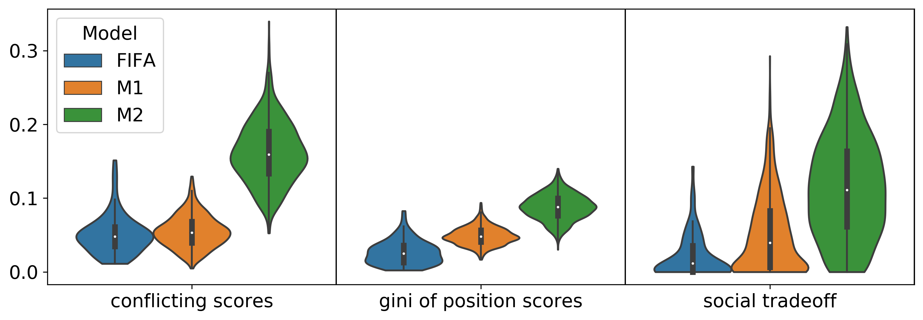
Figure 6: Comparison of different models to generate ten-candidates ten-positions elections.

B.5 Missing Experimental Results for M1 Model

In Figure 10, we present a comparison of the different voting rules on M1 and FIFA data for ten players on ten positions. Note that while the general trends are similar on both data sets, all voting rules produce slightly worse results on the M1 data. Moreover, the difference between the voting rules is more profound on the M1 data.

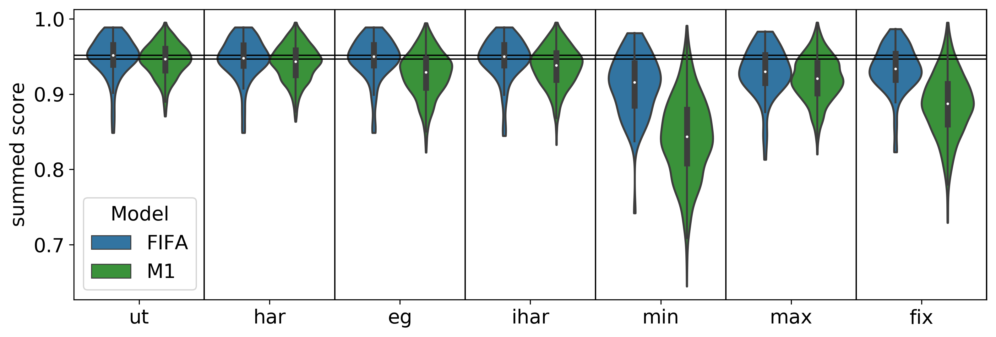
(a) Summed score.

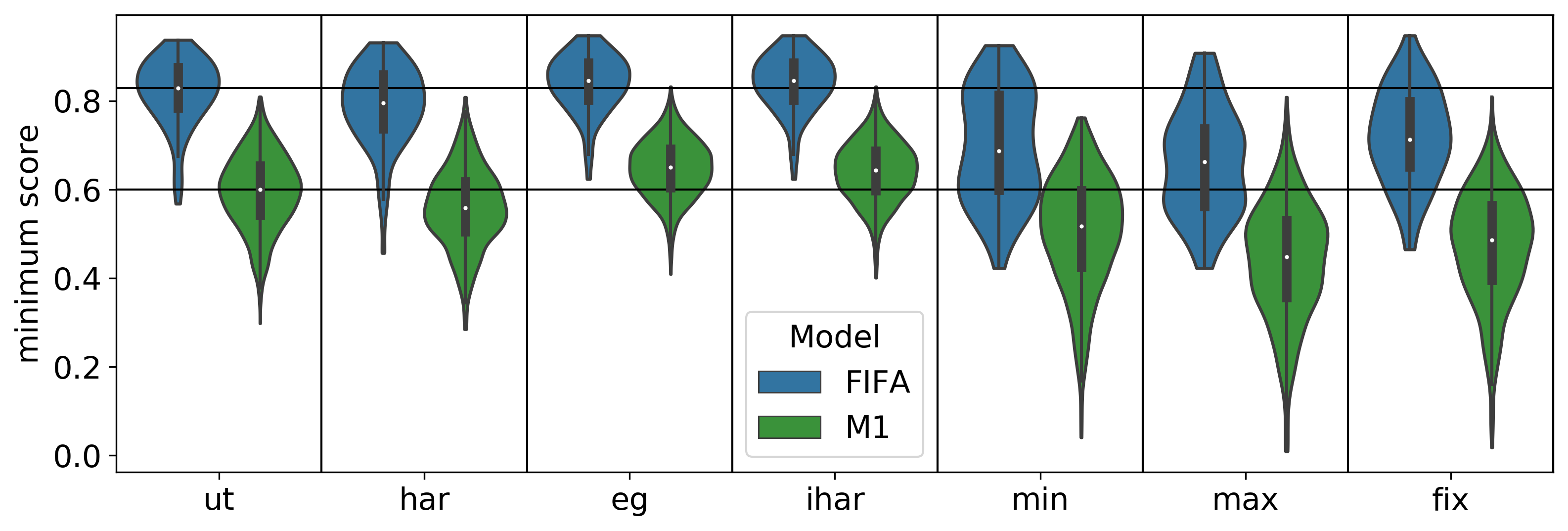
(a) Minimum score.

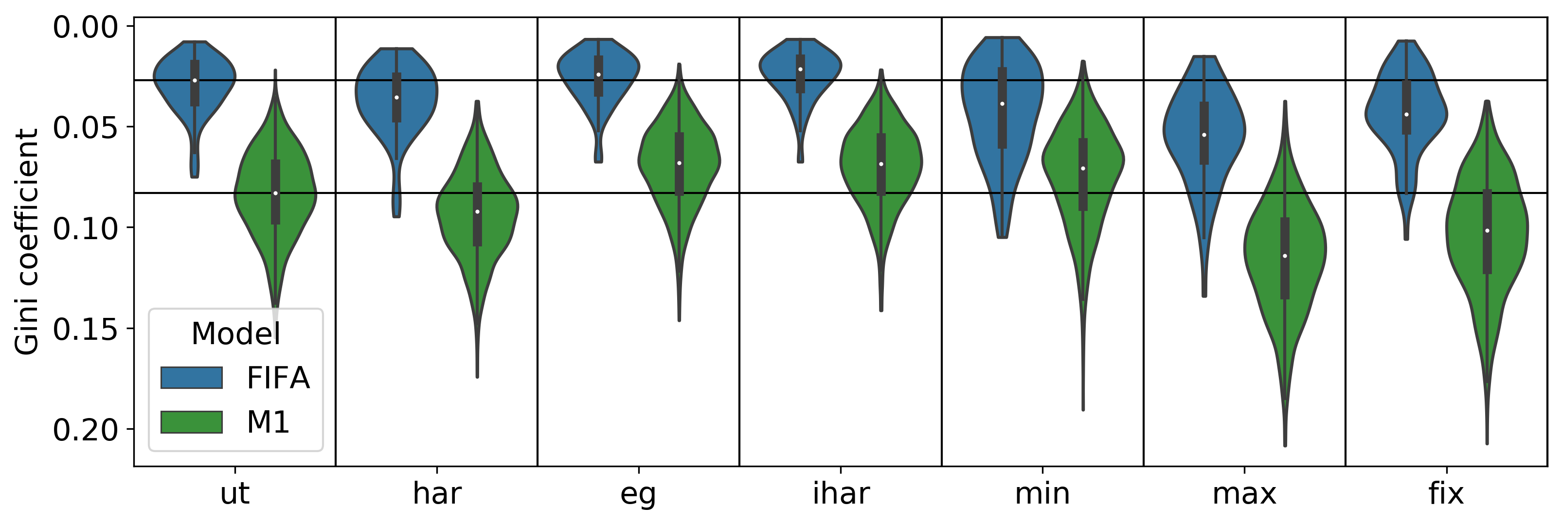
(a) Gini coefficient of score vector.

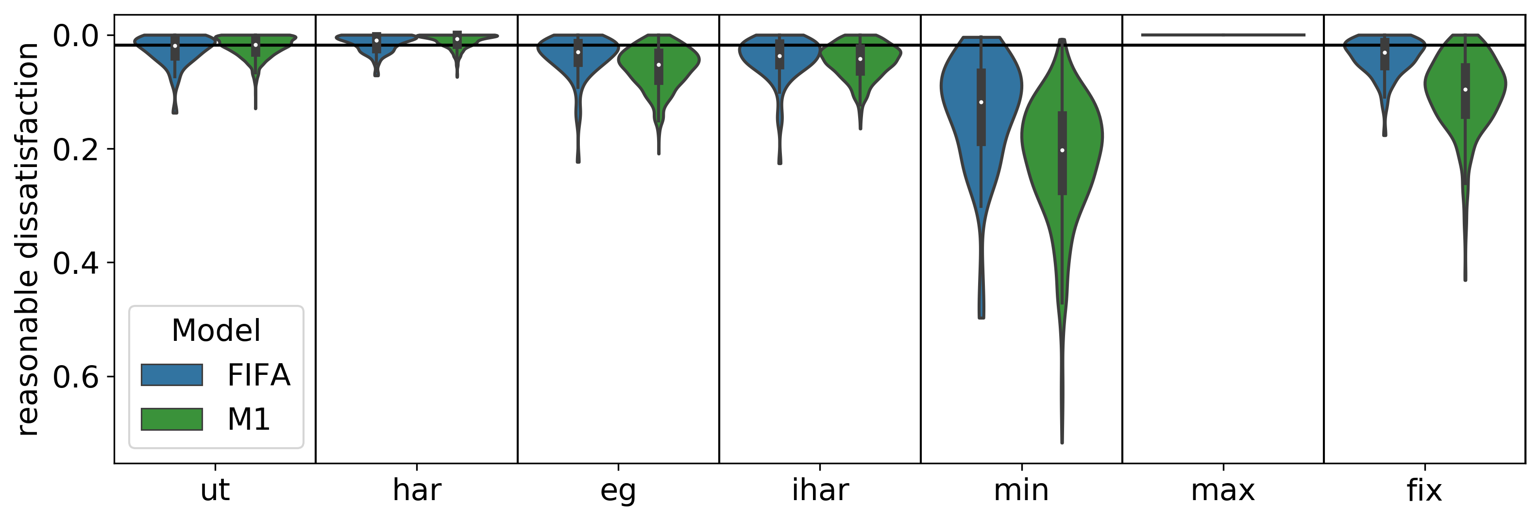
(a) Reasonable dissatisfaction.

Figure 10: Comparison of voting rules on M1 and FIFA data.

B.6 Additional Experimental Results

We also conducted experiments varying the number of positions and candidates. In the following, we exemplarily include our results for the case with twenty candidates on ten positions and twenty candidates on twenty positions.

B.6.1 Twenty candidates on ten positions

Here, diagrams for our experiments with twenty candidates on ten positions are displayed. In Figure 11, instances produced by the three different models are compared to each other. Note that the general picture is similar to the comparison of the models for ten-candidates ten-positions elections (see Figure 6). However, here, due to the higher number of available candidates, the instances exhibit less competition, as overall twenty-candidates ten-positions instances have lower conflicting score, Gini coefficient, and social conflict than ten-candidates ten-positions elections. Moreover, in Figure 15, the performance of the considered voting rules with respect to the summed score of a line-up, the minimum score in a line-up, the Gini coefficient of the score vector, and the reasonable dissatisfaction in a line-up are shown. Note that the general trends highlighted in the main body of the paper still hold while being less visible due to less competition in the data.

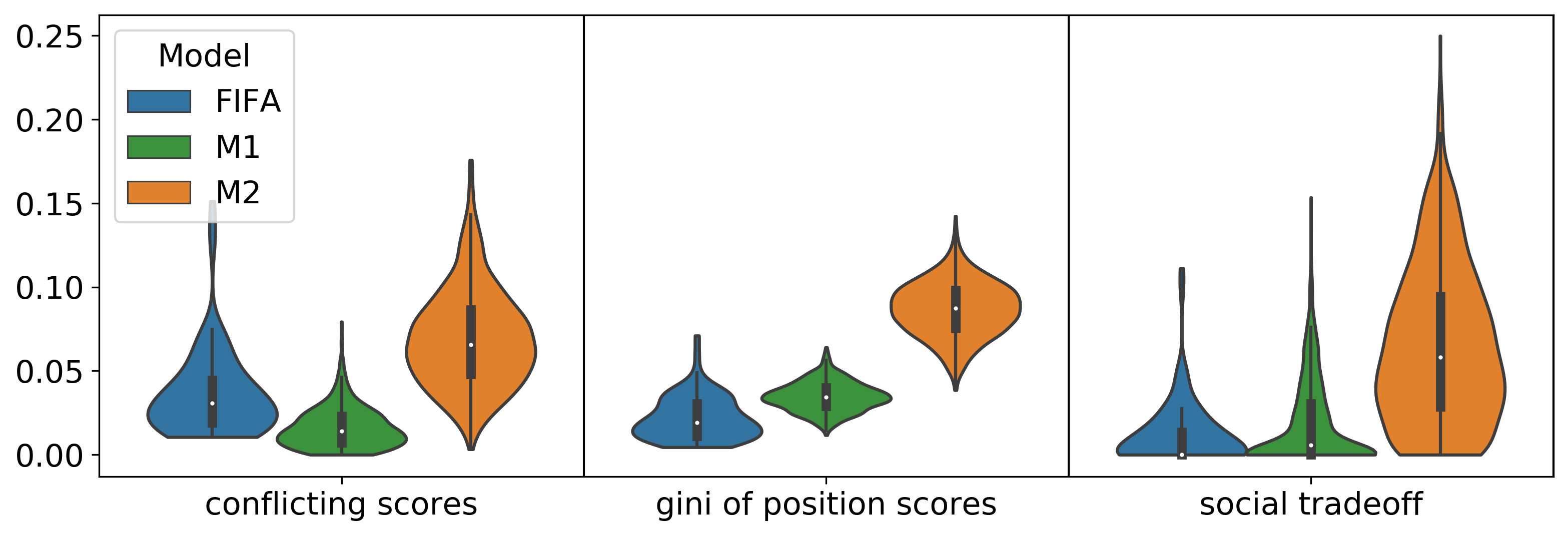
Figure 11: Comparison of different models to generate twenty-candidates ten-positions elections.

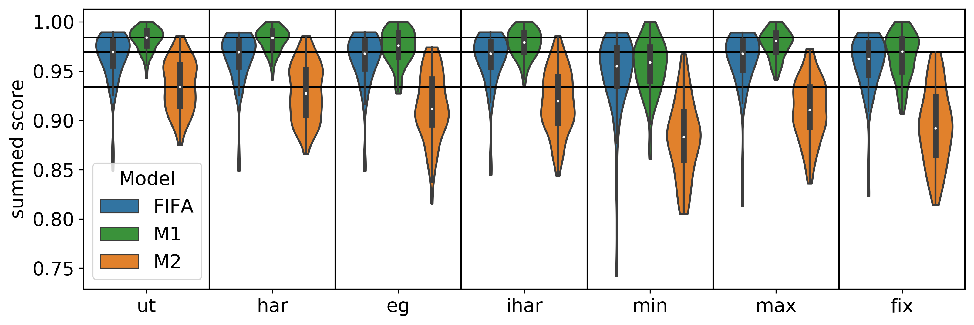
(a) Summed score.

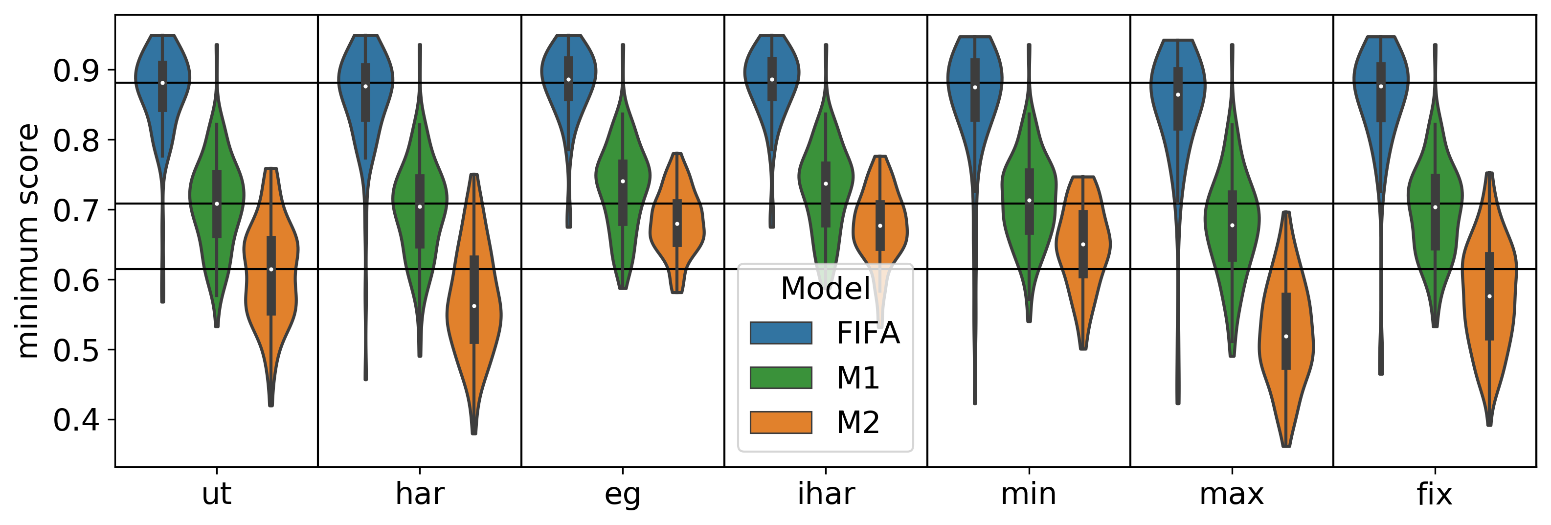
(a) Minimum score.

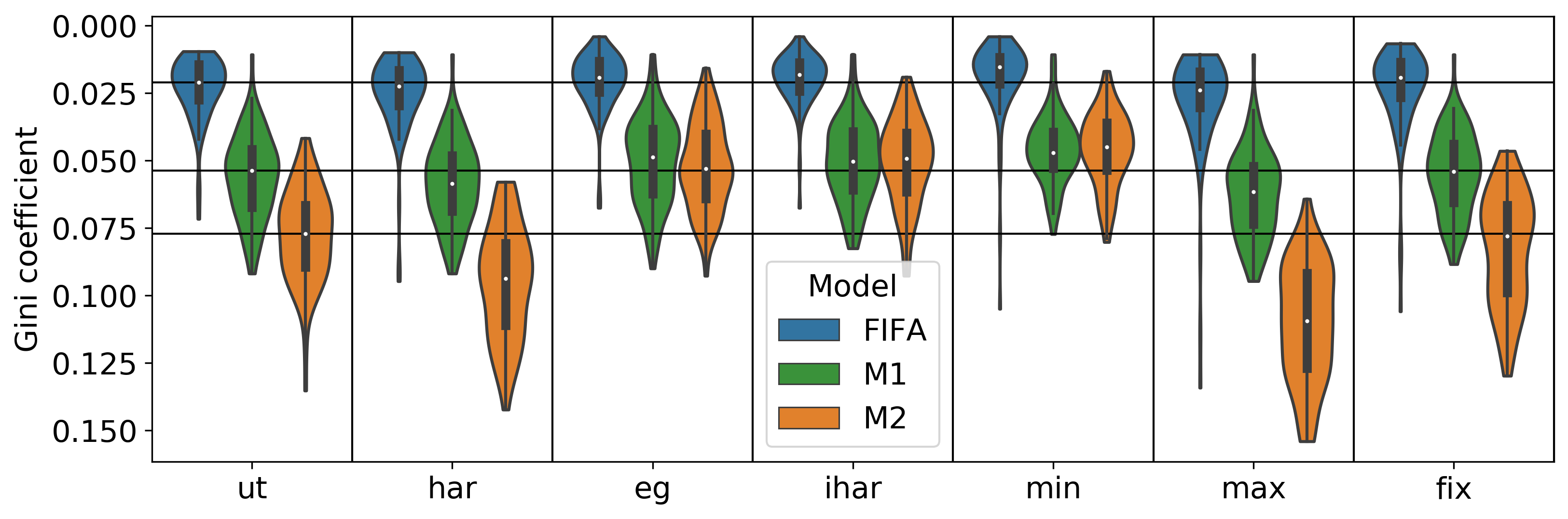
(a) Gini coefficient of score vector.

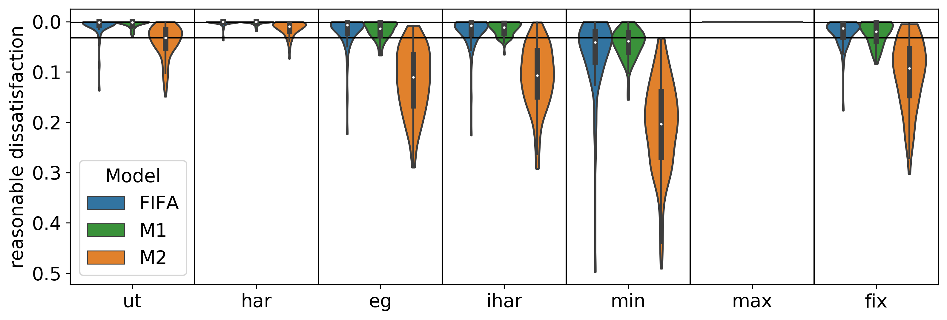
(a) Reasonable dissatisfaction.

Figure 15: Comparison of voting rules on twenty-candidates ten-positions elections using M1, M2, and FIFA data.

B.6.2 Twenty candidates on twenty positions

In the following, diagrams presenting our results for experiments with twenty candidates on twenty positions are shown. We did not use our FIFA data for these experiments, as in soccer line-ups consist only of ten (or eleven) positions. Moreover, due to limited computation time, we did not run the experiments in this setting for the inverse harmonic rule. That is why we omit this rule in all diagrams.

In Figure 16, the instances produced by the three different models are compared to each other. Considering the selected three metrics, the generated twenty-candidates twenty-positions instances seem to be pretty similar to the generated ten-candidates ten-positions instances. Additionally, the outcomes produced by all voting rules except the inverse harmonic rule are analyzed in Figure 15. Again, the results are pretty similar to the ten-candidates ten-positions case discussed in the main body of the paper.

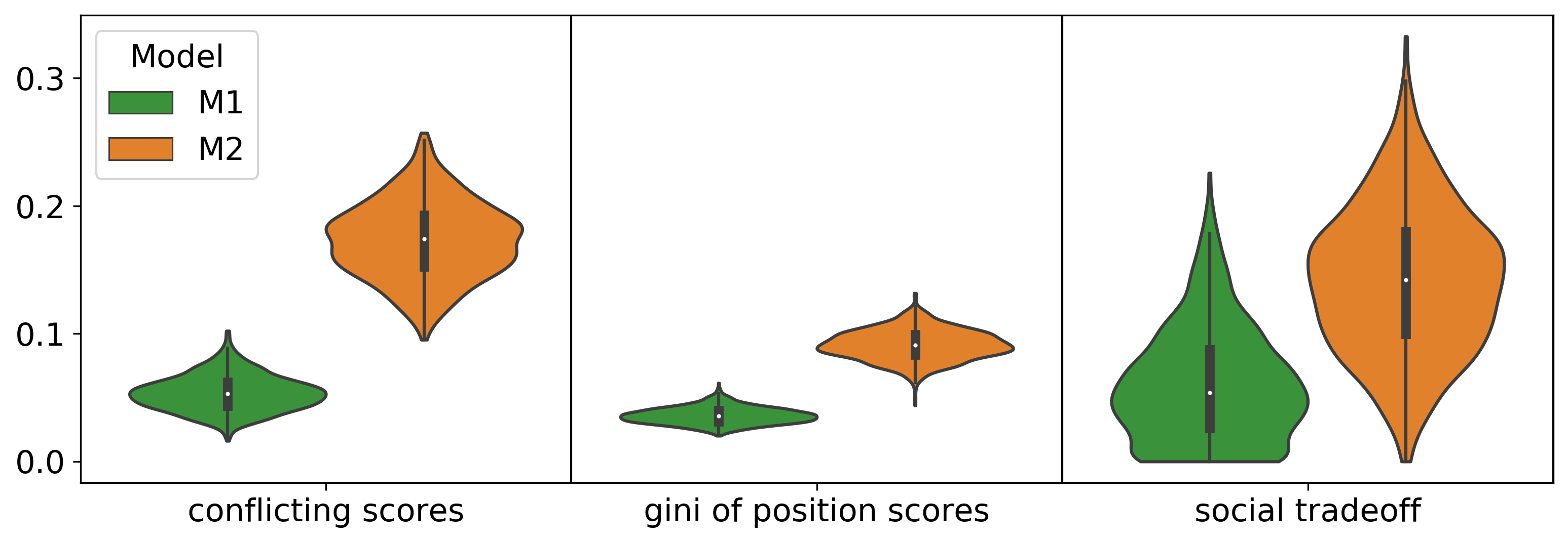
Figure 16: Comparison of different models to generate twenty-candidates twenty-positions elections.

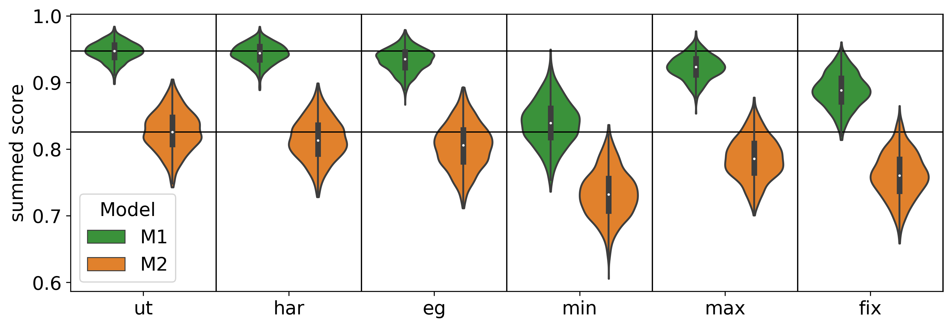
(a) Summed score.

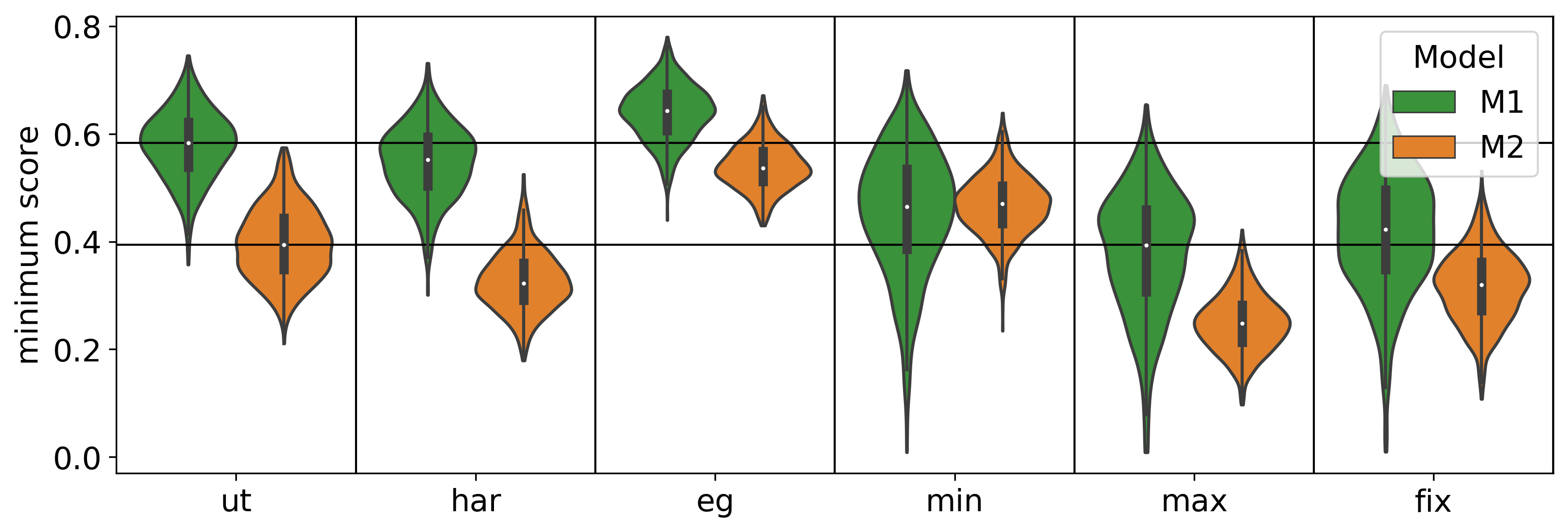
(a) Minimum score.

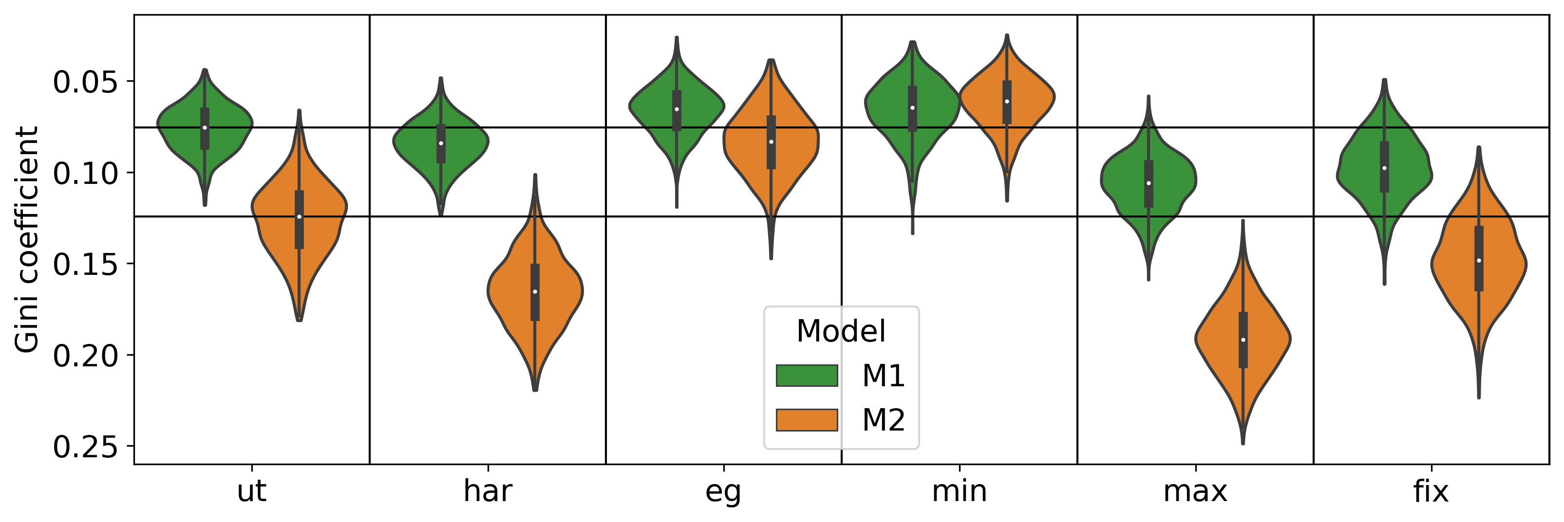
(a) Gini coefficient of score vector.

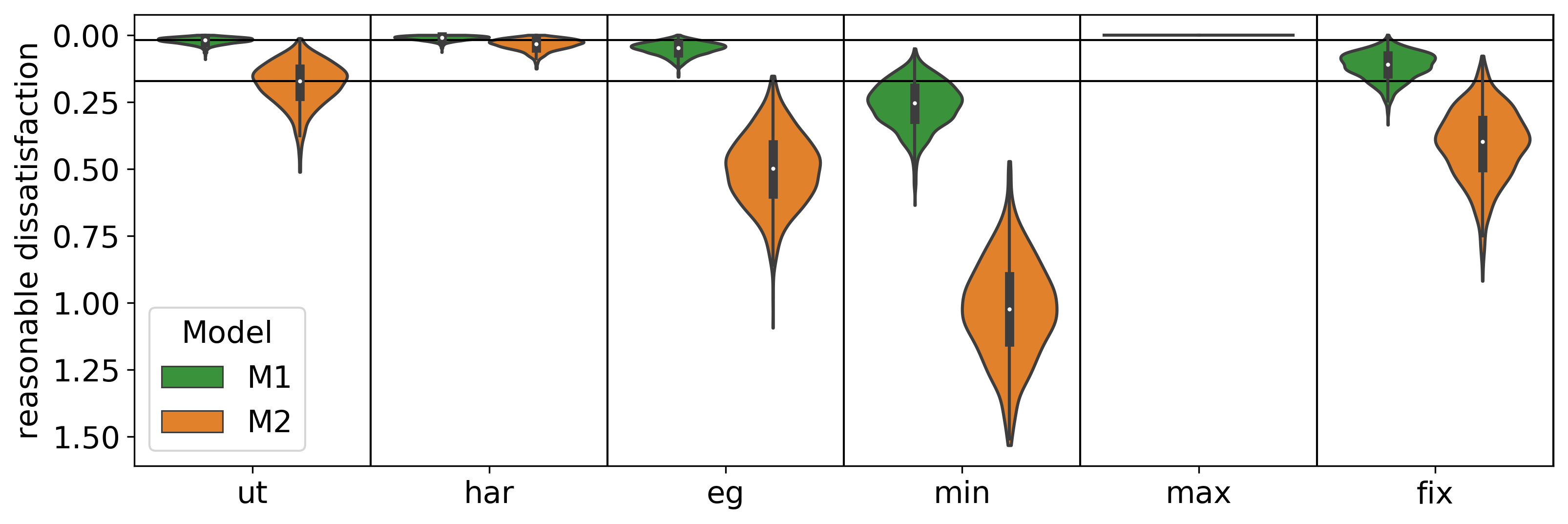
(a) Reasonable dissatisfaction.

Figure 20: Comparison of voting rules on twenty-candidates twenty-positions elections using M1 and M2 data.

References

- [1] Anshelevich, E., Dasgupta, A., Kleinberg, J.M., Tardos, É., Wexler, T., Roughgarden, T.: The price of stability for network design with fair cost allocation. SIAM J. Comput. 38(4), 1602–1623 (2008)
- [2] Arrow, K.J., Sen, A., Suzumura, K. (eds.): Handbook of social choice and welfare, vol. 2. Elsevier (2010)
- [3] Avis, D.: A survey of heuristics for the weighted matching problem. Networks 13(4), 475–493 (1983)
- [4] Aziz, H., Brill, M., Conitzer, V., Elkind, E., Freeman, R., Walsh, T.: Justified representation in approval-based committee voting. Soc. Choice Welf. 48(2), 461–485 (2017)
- [5] Aziz, H., Gaspers, S., Gudmundsson, J., Mackenzie, S., Mattei, N., Walsh, T.: Computational aspects of multi-winner approval voting. In: AAMAS ’15. pp. 107–115 (2015)
- [6] Aziz, H., Lee, B.E.: Sub-committee approval voting and generalized justified representation axioms. In: AIES ’18. pp. 3–9 (2018)
- [7] Barberà, S., Coelho, D.: How to choose a non-controversial list with names. Soc. Choice Welf. 31(1), 79–96 (2008)
- [8] Brams, S.J., Fishburn, P.C.: Voting procedures. In: Handbook of Social Choice and Welfare, chap. 4, pp. 173–236 (2002)
- [9] Bredereck, R., Faliszewski, P., Kaczmarczyk, A., Knop, D., Niedermeier, R.: Parameterized algorithms for finding a collective set of items. In: AAAI ’20. pp. 1838–1845 (2020)
- [10] EA Sports: FIFA 19. [CD-ROM] (2018)
- [11] Elkind, E., Faliszewski, P., Skowron, P., Slinko, A.: Properties of multiwinner voting rules. Soc. Choice Welf. 48(3), 599–632 (2017)
- [12] Elkind, E., Ismaili, A.: OWA-based extensions of the Chamberlin-Courant rule. In: ADT ’15. pp. 486–502 (2015)
- [13] Faliszewski, P., Skowron, P., Slinko, A., Talmon, N.: Multiwinner voting: A new challenge for social choice theory. In: Trends in Computational Social Choice, pp. 27–47 (2017)
- [14] Fishburn, P.C.: Monotonicity paradoxes in the theory of elections. Discrete Appl. Math. 4(2), 119–134 (1982)
- [15] Gadiya, K.: FIFA 19 complete player dataset (2019), https://www.kaggle.com/karangadiya/fifa19
- [16] Gale, D., Shapley, L.S.: College admissions and the stability of marriage. Am. Math. Mon. 69(1), 9–15 (1962)
- [17] Garfinkel, R.S.: Technical note - An improved algorithm for the bottleneck assignment problem. Oper. Res. 19(7), 1747–1751 (1971)
- [18] Garg, N., Kavitha, T., Kumar, A., Mehlhorn, K., Mestre, J.: Assigning papers to referees. Algorithmica 58(1), 119–136 (2010)
- [19] Golden, B., Perny, P.: Infinite order Lorenz dominance for fair multiagent optimization. In: AAMAS ’10. pp. 383–390 (2010)
- [20] Goldsmith, J., Sloan, R.: The AI conference paper assignment problem. In: MPREF ’07 (2007)
- [21] Kuhn, H.W.: The hungarian method for the assignment problem. In: 50 Years of Integer Programming, pp. 29–47 (2010)
- [22] Lang, J., Xia, L.: Sequential composition of voting rules in multi-issue domains. Math. Soc. Sci. 57(3), 304–324 (2009)
- [23] Lesca, J., Minoux, M., Perny, P.: The fair OWA one-to-one assignment problem: NP-hardness and polynomial time special cases. Algorithmica 81(1), 98–123 (2019)
- [24] Lian, J.W., Mattei, N., Noble, R., Walsh, T.: The conference paper assignment problem: Using order weighted averages to assign indivisible goods. In: AAAI ’18. pp. 1138–1145 (2018)
- [25] Murphy, R.: FIFA player ratings explained. https://www.goal.com/en-ae/news/fifa-player-ratings-explained-how-are-the-card-number-stats/1hszd2fgr7wgf1n2b2yjdpgynu (2018), accessed: 2020-07-08
- [26] Skowron, P., Faliszewski, P., Lang, J.: Finding a collective set of items: From proportional multirepresentation to group recommendation. Artif Intell 241, 191–216 (2016)
- [27] Yager, R.R.: On ordered weighted averaging aggregation operators in multicriteria decisionmaking. IEEE Trans. Syst. Man Cybern. Syst. 18(1), 183–190 (1988)
- [28] Young, H.: An axiomatization of Borda’s rule. J. Econ. Theory 9(1), 43 – 52 (1974)
- [29] Zwicker, W.S.: Introduction to the theory of voting. In: Handbook of Computational Social Choice, pp. 23–56 (2016)