On Wiener’s Violent Oscillations, Popov’s curves and Hopf’s Supercritical Bifurcation for a Scalar Heat Equation

Abstract.

A parameter dependent perturbation of the spectrum of the scalar Laplacian is studied for a class of nonlocal and non-self-adjoint rank one perturbations. A detailed description of the perturbed spectrum is obtained both for Dirichlet boundary conditions on a bounded interval as well as for the problem on the full real line. The perturbation results are applied to the study of a related parameter dependent nonlinear and nonlocal parabolic equation. The equation models a feedback system that e.g. can be interpreted as a thermostat device or in the context of an agent based price formation model for a market. The existence and the stability of periodic self-oscillations of the related nonlinear and nonlocal heat equation that arise from a Hopf bifurcation is proved. The bifurcation and stability results are obtained both for the nonlinear parabolic equation with Dirichlet boundary conditions and for a related problem with nonlinear Neumann boundary conditions that model feedback boundary control. The bifurcation and stability results follow from a Popov criterion for integral equations after reducing the stability analysis for the nonlinear parabolic equation to the study of a related nonlinear Volterra integral equation. While the problem is studied in the scalar case only it can be extended naturally to arbitrary euclidean dimension and to manifolds.

1. Introduction

In [14] the authors consider a simple model of a one-dimensional temperature control system given by

(1.1) $$\begin{cases}u_{t}-u_{xx}=0&\text{in }(0,\infty)\times(0,\pi),\\ u_{x}(t,0)=\tanh\bigl{(}\beta u(t,\pi)\bigr{)}&\text{for }t\in(0,\infty),\\ u_{x}(t,\pi)=0&\text{for }t\in(0,\infty),\\ u(0,\cdot)=u_{0}&\text{in }(0,\pi),\end{cases}$$

where heat is injected/removed from the interval $[0,\pi]$ at the left endpoint $x=0$ based on a temperature measurement taken at the other endpoint $x=\pi$. The system is controlled by the parameter $\beta>0$ which models the intensity of the heat injection/removal. The trivial solution $u\equiv 0$ represents the desired equilibrium state of the system. As it turns out, it can only be obtained with certainty (and independently of the initial state) up to the critical parameter value $\beta_{0}\approx 5.6655$, at which a Hopf bifurcation occurs causing the loss of linear stability of the trivial steady-state and the appearance of periodic solutions. The problem first introduced in [14] was inspired by a remark in N. Wiener’s book “Cybernetics” on possible violent temperature oscillations for a badly designed thermostat device that is quoted in [14]. Subsequently the problem received attention in a series of papers [9], [7], [8], [17], [18], [19], [23] mainly due to its novelty and the interesting properties hidden behind its apparent simplicity.
The Hopf bifurcation phenomenon engendered by the nonlocal nature of the boundary condition has also inspired an application, presented in [13], to a market price formation model introduced by J.M. Lasry and P.L. Lions. In particular, in that specific context a similar Hopf bifurcation scenario shows that “demand” and “supply” do not simply lead to unique equilibrium prices but can produce price oscillations. The phenomenon emerges on the basis of the modelled behaviour of the population densities of buyers and sellers positioned in a liquid market over a continuum of prospective transaction prices.
Problem (1.1) can be conventiently weakly formulated as the abstract Cauchy problem

$$\begin{cases}\dot{u}+Au=-\tanh\bigl{(}\beta u(t,\pi)\bigr{)}\delta_{0},&t>0,\\ u(0)=u_{0},&\end{cases}$$

in the space $\operatorname{H}^{-1}=\operatorname{H}^{1}(0,\pi)^{\prime}$, where the unbounded operator $A$ defined on $\operatorname{H}^{-1}$ and with domain $\operatorname{dom}(A)=\operatorname{H}^{1}(0,\pi)$ is the one induced by the Dirichlet form $a(u,v)=\int_{0}^{\pi}u_{x}v_{x}\,dx$ defined on the product space $\operatorname{H}^{1}(0,\pi)\times\operatorname{H}^{1}(0,\pi)$. We refer to [14] and [15] for additional details.

In this paper, taking inspiration from that model we consider the following heat conduction problem

(1.2) $$\begin{cases}u_{t}+A_{L}u=-f\bigl{(}\beta\langle\delta_{x_{0}},u\rangle\bigr{)}\delta_{0},&t>0,\\ u(0)=u_{0},&\end{cases}$$

for the unbounded operator $A_{L}:\operatorname{H}^{1}_{L}\subset\operatorname{H}^{-1}_{L}\to\operatorname{H}^{-1}_{L}$, where it holds that $\operatorname{H}^{1}_{L}:=\operatorname{H}^{1}_{0}\bigl{(}(-L,L)\bigr{)}$ and that $\operatorname{H}^{-1}_{L}:=\operatorname{H}^{1}_{0}\bigl{(}(-L,L)\bigr{)}^{\prime}=\operatorname{H}^{-1}\bigl{(}(-L,L)\bigr{)}$, and where $A_{L}$ is the operator induced by the Dirichlet form

$$a:\operatorname{H}^{1}_{L}\times\operatorname{H}^{1}_{L}\to\mathbb{R},\>(u,v)\mapsto a(u,v)=\int_{-L}^{L}u_{x}v_{x}\,dx$$

on the interval $(-L,L)$ with $L\in(0,\infty]$ and for a smooth bounded globally Lipschitz non-linearity $f$ satisfying the conditions $f(0)=0$, $f^{\prime}(0)=1$, and $\operatorname{sign}(f)=\operatorname{sign}(\operatorname{id}_{\mathbb{R}})$. We also assume, without loss of any generality, that $x_{0}\in(0,L)$. The Cauchy problem (1.2) can be thought of as a heat conduction model with a source placed in the origin which is controlled by a temperature measurement at another point $x_{0}$ in the domain.
The rest of the paper is organized as follows. Sections 2 and 3 are devoted to the study of the linear problems for $L=\infty$ and $L<\infty$, respectively. In particular, a detailed understanding of the dependence of the spectrum of $A_{\beta,L}=A_{L}+\beta\delta_{0}\delta_{x_{0}}^{\top}$ on the parameter $\beta$ is obtained. The main results of this paper require the preparatory ground work of Section 4 on the instrumental Volterra integral equation associated with (1.2). They are given in Section 5, Theorem 5.2 for the Volterra integral equation and, in Section 6, Theorems 6.2 and 6.5, for the nonlinear heat equation (1.2). In Section 6 we also state Theorem 6.7 that settles a conjecture of [14] and that motivates the approach described in [16] and the analysis performed in the present article. The main results are valid for $L<\infty$ only. The case when $L=\infty$ poses additional difficulties and may be the subject of further research. One difficulty incurred when $L=\infty$ is the fact that the continuous spectrum of the linearization is not bounded away from the imaginary axis. Nevertheless a partial investigation of the case $L=\infty$ is included since it is simpler, in certain aspects, and contributes to the understanding of the case $L<\infty$.

2. The Linear Problem on the Real Line

We first consider the linearized problem obtained by choosing $f=\operatorname{id}_{\mathbb{R}}$. This amounts to understanding the operator

(2.1) $$A_{L,\beta}=A_{L}+\beta\delta_{0}\delta_{x_{0}}^{\top}:\operatorname{H}^{1}_{L}\subset\operatorname{H}^{-1}_{L}\to\operatorname{H}^{-1}_{L},$$

where we use the suggestive notation $\delta_{x_{0}}^{\top}$ for the trace/evaluation operator $\gamma_{x_{0}}$ at the point $x_{0}$. The operator $A_{L,\beta}$ is a relatively bounded rank one perturbation of $A_{L}$ by $B=\beta\delta_{0}\delta_{x_{0}}^{\top}$, for which it is well-known that $-A_{L}$ generates an analytic $c_{0}$-semigroup $T_{L}(t)=e^{-tA_{L}}$ on $\operatorname{H}^{-1}_{L}$. When the case $L=\infty$ is considered, the index will be dropped for simplicity so that, e.g., $A$ and $\operatorname{H}^{\pm 1}$ will be used instead of $A_{\infty}$ and $\operatorname{H}^{\pm 1}_{\infty}$, if a more consistent notation were to be applied. When $L=\infty$, it is well-known that

$$e^{-tA}u_{0}=\frac{1}{\sqrt{4\pi t}}e^{-\frac{|\cdot|^{2}}{4t}}*u_{0},\>u_{0}\in\operatorname{L}^{1}(\mathbb{R}),$$

whereas the case $L<\infty$ will be discussed in more detail later. The perturbation $B$ satisfies

$$B\in\mathcal{L}\bigl{(}\operatorname{H}^{\frac{1}{2}+\varepsilon}_{L},\operatorname{H}^{-\frac{1}{2}-\varepsilon}_{L}\bigr{)},$$

for any $\varepsilon\in(0,\frac{1}{2}]$ and any $L\in(0,\infty]$, due to the embedding $\operatorname{H}^{\frac{1}{2}+\varepsilon}_{L}\hookrightarrow\operatorname{BUC(-L,L)}$ and due to $\delta_{0}\in\operatorname{H}^{-\frac{1}{2}-\varepsilon}_{L}$. The notation $\operatorname{BUC}(-L,L)$ refers to the space of bounded and uniformly continuous real-valued functions defined on $(-L,L)$. The following simple remark is useful for the case $L=\infty$.

Remark 2.1.

It holds that $\operatorname{H}^{1}\hookrightarrow\operatorname{C}_{0}(\mathbb{R})$. This follows from the fact that $(1+|\cdot|^{2})^{\frac{1}{2}}\hat{u}\in\operatorname{L}^{2}(\mathbb{R})$ by the definition of $\operatorname{H}^{1}$, which, in turn yields

$$\int|\hat{u}(\xi)|\,d\xi\leq\bigl{[}\int(1+|\xi|^{2})|\hat{u}(\xi)|^{2}\,d\xi\bigr{]}^{\frac{1}{2}}\bigl{[}\int\frac{1}{1+|\xi|^{2}}\,d\xi\bigr{]}^{\frac{1}{2}}\leq c\|u\|_{\operatorname{H}^{1}}$$

The Riemann-Lebesgue Lemma then gives the claimed embedding since

$$u=\mathcal{F}^{-1}(\hat{u})=\widetilde{\mathcal{F}(\hat{u})},$$

where $\tilde{f}(x):=f(-x)$ and $\hat{f}(\omega)\equiv\mathcal{F}(f)(\omega):=\int e^{-ix\omega}f(x)\,dx$ is the standard Fourier transform.

Returning to the operator $B$, we see that it is indeed a relatively bounded perturbation thanks to the interpolation inequality for Bessel potential spaces which yields

$$\|Bu\|_{\operatorname{H}^{-1}_{L}}\leq c\,|u(x_{0})|\leq c\,\|u\|_{\operatorname{H}^{\frac{1}{2}+\varepsilon}_{L}}\leq c\,\|u\|_{\operatorname{H}^{-1}_{L}}^{\frac{1}{4}+2\varepsilon}\|u\|_{\operatorname{H}^{1}_{L}}^{\frac{3}{4}-2\varepsilon}\leq\delta\|u\|_{\operatorname{H}^{1}_{L}}+c_{\delta}\|u\|_{\operatorname{H}^{-1}_{L}},$$

which is valid for any $\delta>0$ by appropriate choice of the constant $c_{\delta}>0$. It then follows from a classical perturbation result for generators of analytic semigroups (see [21, Theorem 2.4 on page 499]) that $A_{\beta}$ also generates such a semigroup on $\operatorname{H}^{-1}_{L}$ for any $\beta\in\mathbb{R}$. In [10], Desch and Schappacher show directly that relatively bounded rank one perturbations of generators of analytic $c_{0}$-semigroups preserve the generation property. They also show that this is not the case for non-analytic semigroups and, in fact, leads to an alternative characterization of analyticity of a semigroup. Later in [5], Arendt and Randy show that positive rank one perturbations of the generator of a holomorphic semigroup preserve not only the generation property but also positivity. They approach the problem via resolvent positivity which, for a given linear operator $C:\operatorname{dom}(C)\subset E\to E$ amounts to the validity of

$$(\lambda-C):\operatorname{dom}(C)\to E\text{ is bijective and }(\lambda-C)^{-1}\text{ is positive for }\lambda>\omega,$$

for some $\omega\in\mathbb{R}$ and characterizes positivity of the corresponding semigroup $T_{C}(t)$. This clearly requires $E$ to be a Banach lattice, see [5]. As it is known that $-A$ generates a positive semigroup, we see that the same remains true for $-A_{\beta}$ for any $\beta<0$. We are, however, interested in the parameter range $\beta>0$. It is therefore natural to ask whether the semigroups remains positive for any parameter value in this regime.

Proposition 2.2.

Let $\beta>0$. Then $-A_{\beta}$ is not resolvent positive and, consequently, the corresponding semigroup $T_{A_{\beta}}$ is not positive.

Proof.

The space $\operatorname{H}^{1}$ becomes a Banach lattice if one defines

$$u\geq 0\text{ iff }u(x)\geq 0\text{ for }x\in\mathbb{R}.$$

This follows from the continuity of any $u\in\operatorname{H}^{1}$. One can then make $\operatorname{H}^{-1}$ into a Banach lattice as well by defining

$$T\geq 0\text{ iff }\langle T,u\rangle\geq 0\text{ for every }u\geq 0,$$

for any given $T\in\operatorname{H}^{-1}$. Next notice that the resolvent equation for $-A_{\beta}$, given by

$$(s+A_{\beta})u=(s+A)u+\beta u(x_{0})\delta_{0}=f,$$

can be solved for $u$ by observing that

$$u=(s+A)^{-1}f-\beta u(x_{0})(s+A)^{-1}\delta_{0}\,.$$

Then, evaluating the last expression at $x_{0}\,$, solving for $u(x_{0})$, and reinserting the result back into the formula above, one obtains

$$u=(s+A_{\beta})^{-1}f=(s+A)^{-1}f-\beta\frac{\bigl{[}(s+A)^{-1}f\bigr{]}(x_{0})}{1+\beta\bigl{[}(s+A)^{-1}\delta_{0}\bigr{]}(x_{0})}(s+A)^{-1}\delta_{0},$$

for any $s>0\,$. More precisely, this holds for $s\,\in\,\rho(-A)\cap\rho(-A_{\beta})\,$, where $\rho(-A)$ and $\rho(-A_{\beta})$ denote the resolvent set of $-A$ and $-A_{\beta}\,$, respectively. It will be shown later that

$$\rho(-A)\cap\rho(-A_{\beta})=\rho(-A_{\beta})\supset(0,\infty).$$

Also observe that $(s+A)^{-1}=\text{``}(s-\partial_{xx})^{-1}\text{''}$ is given by convolution with the kernel

(2.2) $$G_{s}(x)=\frac{1}{2\sqrt{s}}\;e^{-\sqrt{s}\,|x|}\;,$$

whenever the convolution makes sense. Now take $f=\delta_{y}$ for $y\in\mathbb{R}$ to be determined later. Then the solution of $(s+A_{\beta})u=f$ is given by

(2.3) $$u(x)=G_{s}(x-y)-\beta\frac{G_{S}(x_{0}-y)}{1+\beta G_{s}(x_{0})}G_{s}(x),\>x\in\mathbb{R}\;,$$

so that

$$u(0)=\frac{1}{2\sqrt{s}}e^{-\sqrt{s}|y|}-\beta\frac{\frac{1}{2\sqrt{s}}e^{-\sqrt{s}|x_{0}-y|}}{1+\frac{\beta}{2\sqrt{s}}e^{-\sqrt{s}|x_{0}|}}\;.$$

Setting $y=x_{0}$ one gets that

$$u(0)=\frac{1}{2\sqrt{s}}e^{-\sqrt{s}|x_{0}|}\Bigl{(}1-\beta\frac{e^{\sqrt{s}|x_{0}|}}{1+\frac{\beta}{2\sqrt{s}}e^{-\sqrt{s}|x_{0}|}}\Bigr{)}.$$

As long as $\beta>0$, it follows that $u(0)<0$ for $s\geq s_{0}>0$ and some $s_{0}>0$ and, since $u\in\operatorname{H}^{1}$, also that $u\not\geq 0$, showing that

$$(s+A)^{-1}\delta_{x_{0}}\not\geq 0\text{ for }s\geq s_{0},$$

and the claim follows since $\delta_{x_{0}}\geq 0$ in $\operatorname{H}^{-1}$. ∎

Remark 2.3.

We will analyze the operator $A_{L,\beta}$ ($L<\infty$) later, in which case the above proposition remains valid. In that case, however, a weaker positivity property holds up to a critical value $\beta_{+}>0$.

By providing a careful spectral analysis of the operator $A_{\beta}$, it will be shown below that, not only positivity is lost but, in fact, (1.2) possesses oscillatory solutions.

Remark 2.4.

While $-A_{L,\beta}$ ($L\in(0,\infty]$) generates a holomoprhic semigroup, the solutions of the linear Cauchy problem are not smooth, since any solution $u$ will clearly have non-differentiable derivatives whenever $u(x_{0})\neq 0$, as follows from the fact that

$$u_{t}-u_{xx}=-\beta u(x_{0})\delta_{0}.$$

Analyticity of the semigroup entails that $e^{-tA_{L,\beta}}\bigl{(}\operatorname{H}^{-1}_{L}\bigr{)}\subset\operatorname{dom}\bigl{(}A_{L,\beta}^{n}\bigr{)}$ for $t>0$ and $n\in\mathbb{N}$ (see [26, 12]). This shows that the singularity of a solution $e^{-tA_{\beta,L}}u_{0}$ does not deteriorate as more derivatives are taken in the sense that

$$u\in\operatorname{H}^{1}_{L},\>A_{L}u+\beta u(x_{0})\delta_{0}\in\operatorname{H}^{1}_{L},$$

$$A_{L}\bigl{[}A_{L}u+\beta u(x_{0})\delta_{0}\bigr{]}+\beta\bigl{[}A_{L}u+\beta u(x_{0})\delta_{0}\bigr{]}(x_{0})\delta_{0}\in\operatorname{H}^{1}_{L},\>\dots$$

and that $u\in\operatorname{H}^{m}(\mathbb{R}\setminus\{0\})$ for any $m\in\mathbb{N}$. Thus $u(t,\cdot)\in\operatorname{C}^{\infty}(\mathbb{R}\setminus\{0\})$ for any $t>0$ and for any $u_{0}\in\operatorname{H}^{-1}$, and, consequently also $u\in\operatorname{C}^{\infty}\bigl{(}(0,\infty)\times(\mathbb{R}\setminus\{0\})\bigr{)}$.

For the case $L=\infty$ we obtain the following result on the sprectrum of the perturbed operator. Again the case $L<\infty$ will be considered later. However, for finite $L$ the results of our analysis will not be equally explicit as for $L=\infty\,$. We shall use the notation $\sigma_{p}$ and $\sigma_{c}$ for the point and continuous spectrum, respectively.

Proposition 2.5.

There is a critical value $\beta_{0}=\pi$ such that

$$\sigma(-A_{\beta})=\sigma_{c}(-A_{\beta})=(-\infty,0],\>\sigma_{p}(-A_{\beta})=\emptyset$$

for $\beta\in[0,\beta_{0})$. There is a further critical value $\beta_{1}>\beta_{0}$, whose value can be determined explicitely as $\beta_{1}=\frac{3\pi}{\sqrt{2}}e^{3\pi/4}$ such that for any $\beta\in(\beta_{0},\beta_{1})$ the continous spectrum remains unchanged, i.e.,

$$\sigma_{c}(-A_{\beta})=(-\infty,0],$$

whereas the point spectrum is genuinely complex

$$\sigma_{p}(-A_{\beta})=\big{\{}\lambda_{1,\beta},\dots,\lambda_{n_{\beta},\beta}\}\,\subset\ \mathbb{C}\backslash\mathbb{R}$$

and varies with $\beta\in(\beta_{0},\beta_{1})$. The point spectrum is never empty for $\beta\in(\beta_{0},\beta_{1})$ and consists of finitely many, genuinely complex, isolated eigenvalues that form conjugate pairs in the interior of the left complex half plane.
For $\beta=\beta_{1}$, a first pair of complex conjugate eigenvalues reaches the imaginary axis. The pair crosses into the right complex half plane for $\beta>\beta_{1}$, yet never reaches the positive real axis as $\beta\to\infty$.
As $\beta$ increases beyond $\beta_{1}$, additional pairs of complex conjugate eigenvalues are ejected from the real continuous spectrum into the left complex half-plane and migrate towards the imaginary axis, eventually crossing it, pair after pair. For any finite $\beta>0$, there is only a finite number of conjugate eigenvalue pairs. None of the pairs ever reunites on the positive real axis as $\beta\to\infty$.

Proof.

As previously mentioned, it holds that

$$(s+A_{\beta})^{-1}f=(s+A)^{-1}f-\beta\frac{\bigl{[}(s+A)^{-1}f\bigr{]}(x_{0})}{1+\beta\bigl{[}(s+A)^{-1}\delta_{0}\bigr{]}(x_{0})}(s+A)^{-1}\delta_{0}.$$

This shows that, if $s\in\rho(-A)=\rho(-A_{\beta=0})=\mathbb{C}\setminus(-\infty,0]$, then $s\in\rho(-A_{\beta})$ unless it so happens that $1+\beta\bigl{[}(s+A)^{-1}\delta_{0}\bigr{]}(x_{0})=0$. The latter equation is equivalent to

(2.4) $$2\sqrt{s}+\beta e^{-x_{0}\sqrt{s}}=0$$

thanks to (2.2). Zeros of this equation in $\mathbb{C}\setminus(-\infty,0]$ are simple poles of the resolvent and, as such, are eigenvalues of $-A_{\beta}$. This follows from a classical result found e.g. in [28, Theorem 3 on page 229].
Before tracing the path of the complex conjugate pairs in more detail, we provide a qualitative description of the consequences of varying $\beta$. The function (2.4) is holomorphic in the open domain $G:=\mathbb{C}\setminus(-\infty,0]$ and can be written as $f+g$ for $f=\beta e^{-x_{0}\sqrt{\cdot}}$ and $g=2\sqrt{\cdot}$. Since $f$ never vanishes for $\beta\neq 0$ and since $g$ is bounded on any compact subset $K$ of $G$, it is clear that $\lvert g\rvert$ can be dominated by $\lvert f\rvert$ on any such $K$ by making $\lvert\beta\rvert$ sufficiently large. It follows from Rouché’s Theorem that, for any compact $K\subset G$ with smooth boundary, there exists a $\beta(K)>0$ such that (2.4) has no zeros in $K$ for any $\beta\geq\beta(K)$. An analogous statement for $\beta<0$ clearly also holds. Thus, increasing or decreasing $\beta$, all eigenvalues of $A_{\beta}$ exit from any given compact subset of $G$.
The solutions of (2.4) with $s=-\lvert s\rvert\in(-\infty,0]$ and, consequently, with $\operatorname{Re}(\sqrt{s})=0$ can immediately be obtained from the validity of

$$\operatorname{Re}(e^{-x_{0}\sqrt{s}})=0\text{ and }2\operatorname{Im}(\sqrt{s})+\beta\operatorname{Im}(e^{-x_{0}\sqrt{s}})=0.$$

A separate discussion for positive and negative values of $\beta$ produces all negative real solutions of (2.4) for $\beta\neq 0\,$. They are given by

$$s^{+}_{k}=-\frac{(4k+1)^{2}\pi^{2}}{4x_{0}^{2}}\text{ for }\beta^{+}_{k}=\frac{(4k+1)\pi}{x_{0}}\text{ and }k=0,1,2,\dots$$

and

$$s^{-}_{k}=-\frac{(4k+3)^{2}\pi^{2}}{4x_{0}^{2}}\text{ for }\beta^{-}_{k}=-\frac{(4k+3)\pi}{x_{0}}\text{ and }k=0,1,2,\dots$$

In Section 5, the discussion of the Popov criterion will again reveal this pattern, however along the imaginary axis, where zeros are found in an alternating order and they induce a sequence of increasing positive and decreasing negative values of the parameter $\beta$. This reflects the fact, that for increasingly positive values of $\beta$ or decreasingly negative values of $\beta$, complex conjugate solution pairs of (2.4) migrate away from the negative real axis, where they originate at specific locations, towards the imaginary axis.
We now return to a more precise account of the trajectory traced by the (genuinely) complex conjugate solutions of equation (2.4) in terms of the parameter $\beta$. To that end, we write $\sqrt{s}=\alpha+i\gamma$, where $\alpha>0$ and $\gamma\geq 0$. We can restrict our search in this way since we know that $\alpha-i\gamma$ is also a solution and since we are interested in solutions such that $s\not\in(-\infty,0]$, in which case $\operatorname{Re}(\sqrt{s})\geq 0$. Equation (2.4) can then be rewritten as the system

$$\begin{cases}2\alpha+\beta e^{-\alpha}\cos(\gamma)=0,&\\ 2\gamma-\beta e^{-\alpha}\sin(\gamma)=0.&\end{cases}$$

We now fix $x_{0}=1$ in the rest of the calculation. If $0\neq x_{0}\neq 1$, the same qualitative behavior is observed for any $\beta\neq 0$ simply with different numerical values. It follows from the above system that

$$\frac{\gamma}{\alpha}=-\tan(\gamma),$$

and we look for solutions on lines of the form $\gamma/\alpha=m$, i.e. on lines $\alpha+im\alpha$ with parameter $\alpha$ where $m\in[0,\infty]$. In the extreme case when $m=0$, the equation reads $2\alpha+\beta e^{-\alpha}=0$ and has no solutions for any $\beta>0$. Next let’s fix $\frac{\gamma}{\alpha}=m$, in which case

$$\gamma=-\arctan(m)+k\pi$$

for any integer $k$ such that $\gamma\geq 0$. As $m\in(0,\infty]$, one has that $-\arctan(m)\in[-\frac{\pi}{2},0)$ and thus

$$\gamma=\underset{\gamma_{0}}{\underbrace{-\arctan(m)+\pi}},-\arctan(m)+2\pi,\dots=\gamma_{0},\gamma_{0}+\pi,\gamma_{0}+2\pi,\dots=\gamma_{0},\gamma_{1},\gamma_{2},\dots$$

where $\gamma_{0}\in[\frac{\pi}{2},\pi)$. With $\gamma$ in hand and $\alpha=\gamma/m$ we arrive at

$$2\gamma-\beta e^{-\gamma/m}\sin(\gamma)=0,$$

from which we see that we need only to consider even $k\geq 0$ due to $\sin(\gamma_{0}+\pi)<0$ and the periodicity of $\sin$. This shows that no solution exists unless $\beta\geq\beta_{0}>0$, where $\beta_{0}=2\gamma_{0}e^{\gamma_{0}/m}/\sin(\gamma_{0})$. Notice that, if $\gamma_{0}$ is not a solution, then so aren’t $\gamma_{2k}$ for $k\geq 1$ since

$$2\gamma_{2k}>2\gamma_{0}>\beta e^{-\gamma_{0}/m}\sin(\gamma_{0})>\beta e^{-\gamma_{2k}/m}\sin(\gamma_{2k}),$$

and since $\sin(\gamma_{2k})=\sin(\gamma_{0})$.

The limiting case $m=\infty$ corresponds to looking for real negative solutions of $\eqref{poleEq}$ and was discussed above separately. In that case the equation for $\gamma_{0}$ reduces to $2\gamma_{0}=\beta\sin(\gamma_{0})$ and it has no solution unless $\beta\geq 2\gamma_{0}$, i.e. unless $\beta\geq\pi$ since $\gamma_{0}=\pi/2$ for $m=\infty$. We can also conclude that no solution exists for any $m<\infty$ unless $\beta>\pi$. Next take the case when $m=1$, which corresponds to looking for purely imaginary eigenvalues. The equation then reads

$$2\gamma_{0}=\beta e^{-\gamma_{0}}\sin(\gamma_{0})$$

for $\gamma_{0}=3\pi/4$, which requires

(2.5) $$\beta\geq\beta_{1}=\frac{3\pi}{\sqrt{2}}e^{3\pi/4}\simeq 70.3134$$

for a solution to exist. For $\beta=\beta_{1}$ only one solution is found on the line $\gamma=\alpha$. Let us finally consider the case $m\geq m_{*}>1$ for some fixed $m_{*}$. The equation is

$$2\gamma_{0}=\beta e^{-\gamma_{0}/m}\sin(\gamma_{0})=0,$$

where $\gamma_{0}=\pi-\arctan(m)\leq\pi-\arctan(m_{*})=\gamma_{*}$ satisfies $\gamma_{0}\in(\frac{\pi}{2},\gamma_{*}]$ and $\gamma_{*}<\frac{3\pi}{4}$. Under these circumstances, there is no solution until $\beta$ becomes larger or equal than $2\gamma_{0}e^{\gamma_{0}/m}/\sin(\gamma_{0})$ for $m$ fixed. Clearly $\gamma_{0}$ can be thought of as a function $\gamma_{0}(m)$ of $m$, which is decreasing. It follows that the function

$$\Phi(m)=2\frac{\gamma_{0}(m)e^{\gamma_{0}(m)/m}}{\sin\bigl{(}\gamma_{0}(m)\bigr{)}}$$

is also decreasing in $m$. Thus, when considering the equation $\beta=\Phi(m)\leq\Phi(m_{*})$, we see that, for any given $\beta\leq\Phi(m_{*})$, there exists a unique $m=m(\beta)=\Phi^{-1}(\beta)$. It can be verified that $\Phi^{\prime}(1)\approx-254$ and that

$$\lim_{m\to\infty}\Phi(m)=\pi.$$

We conclude that $\sigma(-A_{\beta})=(-\infty,0]$ for $\beta<\pi\,$. We observe that all negative real solutions are also recovered in this more detailed discussion of the case of interest ($\beta>0$). Indeed, for $\beta=\pi$ and $m=\infty$, one has the appearance of the solution $s^{+}_{1}=(i\frac{\pi}{2})^{2}=-\frac{\pi^{2}}{4}$ of (2.4) on the negative real axis (note that $\gamma_{0}=\frac{\pi}{2}$). The next solution to appear from $m=\infty$ satisfies $2(\gamma_{0}+2\pi)=\beta\sin(\gamma_{0})$ yielding $\beta=5\pi$ and the solution $s^{+}_{2}=-\frac{25\pi^{2}}{4}$ of (2.4). It follows that more and more solutions of (2.4) appear on the negative real axis (with increasing absolute value) as $\beta$ increases, and, due to the monotonicity properties of the function $\Phi$, they all migrate towards the imaginary axis along complex conjugate curves which cross and move beyond it.
It remains to verify that the continuous spectrum persists. This follows from general spectral results which are found in Kato’s book [20, Theorem 5.35 in Chapter IV]. For the specific operator of interest here, it is also possible to give a direct proof, which also produces generalized eigenfunctions.

Consider $\lambda=0$ first and notice that $G=A-|x|/2$ is, for any $A\in\mathbb{R}$, a fundamental solution for $-\partial_{xx}$ and therefore it holds that

$$-\partial_{xx}G+\beta G(x_{0})\delta_{0}=\bigl{(}1+\beta A-|x_{0}|/2\bigr{)}\delta_{0}.$$

Setting $A=|x_{0}|/2-1/\beta$ one obtains $G\in N(-\partial_{xx}+\beta\delta_{0}\delta_{x_{0}}^{\top})$. While $G\notin\operatorname{H}^{1}$, it can be approximated by such functions, showing that $\lambda=0$ is indeed still in the spectrum of $A_{\beta}$ when $\beta>0$. For $\lambda=-\alpha^{2}$ and $\alpha>0$, one similarly observes that $\widetilde{G}_{\alpha}=G_{\alpha}+Ae^{i\alpha x}+Be^{-i\alpha x}$ is a fundamental solution of $-\partial_{xx}-\alpha^{2}$ provided

$$G_{\alpha}(x)=\begin{cases}\frac{1}{2i\alpha}e^{i\alpha x},&x<0,\\ \frac{1}{2i\alpha}e^{-i\alpha x},&x\geq 0,\end{cases}$$

since $Ae^{i\alpha x}+Be^{-i\alpha x}\in N(-\partial_{xx}-\alpha^{2})$. One computes that

$$A_{\beta}\widetilde{G}_{\alpha}=\alpha^{2}\widetilde{G}_{\alpha}+\bigl{[}1+\beta\widetilde{G}_{\alpha}(x_{0})\bigr{]}\delta_{0}.$$

Since it is always possible to choose $A$ and $B$ so that $\widetilde{G}_{\alpha}=-1/\beta$, the claim follows as for $\lambda=0$. ∎

The asymptotic behavior of the semigroup generated by $-A_{\beta}$ and the long time behavior of solutions to the Cauchy problem (1.2) is the focus of the remainder of this section. As in the rest of the section we consider the linear case and, again, postpone the discussion of the case when $L<\infty$ to a later section. Equation (2.3) gives an explicit formula for the Green’s function $G_{s,\beta}$ of the operator $s+A_{\beta}$, so that the Laplace transform $\mathcal{L}(u)=\hat{u}$ of a solution $u$ of the linear version of (1.2) is given by

(2.6) $$\hat{u}(s,x)=\frac{1}{2\sqrt{s}}\int e^{-\sqrt{s}|x-y|}u_{0}(y)\,dy-\beta\frac{\int e^{-\sqrt{s}|x_{0}-y|}u_{0}(y)\,dy}{2\sqrt{s}+\beta e^{-\sqrt{s}|x_{0}|}}\;\frac{1}{2\sqrt{s}}e^{-\sqrt{s}|x|}\;.$$

It holds in particular that

$$\hat{u}(s,x_{0})=\frac{1}{1+\frac{\beta}{2\sqrt{s}}e^{-\sqrt{s}|x_{0}|}}\frac{1}{2\sqrt{s}}\int e^{-\sqrt{s}|x_{0}-y|}u_{0}(y)\,dy.$$

Also notice the classical fact that $\mathcal{L}\bigl{(}\frac{1}{\sqrt{4\pi t}}e^{-\frac{|x|^{2}}{4t}}\bigr{)}(s)=\frac{1}{2\sqrt{s}}e^{-\sqrt{s}|x|}$ for $s\in\mathbb{C}\setminus(-\infty,0]$. It is a well-known fact of semigroup theory [4] that

$$\Bigl{(}\int_{0}^{\infty}e^{-st}T_{A_{\beta}}(t)u_{0}\,dt\Bigr{)}(x)=(s+A_{\beta})^{-1}u_{0}=\int G_{s,\beta}(\cdot,y)u_{0}(y)\,dy,$$

so that the kernel $k_{A_{\beta}}(t)$ of $T_{A_{\beta}}(t)$ is given by

$$k_{A_{\beta}}(t)(x,y)=\mathcal{L}^{-1}\bigl{(}G_{\cdot,\beta}(x,y)\bigr{)}.$$

Proposition 2.6.

For any $u_{0}\in\operatorname{L}^{1}(\mathbb{R})$, so in particular for any $u_{0}\in\operatorname{H}^{1}$, it holds, for any $\beta<\beta_{1}$, that

$$u(t,x_{0})=O(\frac{1}{t})\text{ as }t\to\infty,$$

and that

$$u(t,x)=O(\frac{1}{\sqrt{t}})\text{ as }t\to\infty,$$

for the corresponding solution of the linear Cauchy problem and for $x\neq x_{0}$.

Proof.

Define

$$F(s):=\hat{u}(s,x_{0})=\frac{1}{2\sqrt{s}+\beta e^{-\sqrt{s}|x_{0}|}}\int e^{-\sqrt{s}|x_{0}-y|}u_{0}(y)\,dy$$

and observe that the abscissa of convergence $abs\bigl{[}u(\cdot,x_{0})\bigr{]}$ of $u(\cdot,x_{0})$ is 0, i.e. the integral defining the Laplace transform converges for $\operatorname{Re}(s)>0$, by the explicit representation of $\hat{u}$. Then the well-known inversion theorem for the Laplace transform yields that

$$u(t,x_{0})=\frac{1}{2\pi i}\int_{\delta-i\infty}^{\delta+i\infty}e^{zt}F(z)\,dz,\>t>0,$$

where $\delta>0$. Since $\beta<\beta_{1}$, $F$ is holomorphic in a sector

$$[\,\left|\theta\right|\leq\theta_{\beta}\,]\,\setminus\{0\}\text{ for }\theta_{\beta}>\frac{\pi}{2}+\gamma\text{ and some }\gamma>0,$$

as follows from Proposition 2.5. The path of integration can therefore be deformed into

$$\Gamma_{\varepsilon}=(-\infty,-\varepsilon)e^{-i(\frac{\pi}{2}+\gamma)}\cup\underset{C_{\varepsilon}}{\underbrace{\Big{\{}\varepsilon e^{i\theta}\,\Big{|}\,\theta\in\bigl{[}-\frac{\pi}{2}-\gamma,\frac{\pi}{2}+\gamma\bigr{]}\Big{\}}}}\cup(\varepsilon,\infty)e^{i(\frac{\pi}{2}+\gamma)}$$

without changing the value of the integral. The contribution from the integration over the circular arc $C_{\varepsilon}$ is easily seen to vanish as $\varepsilon\to 0+$, so that we can simply integrate along the rays $(-\infty,0)e^{\mp i(\frac{\pi}{2}+\gamma)}$. The estimates of the integrals along both rays can be handled similarly and we therefore only consider one of them. Let $z=r\,e^{i(\frac{\pi}{2}+\gamma)}$ for $r\in(0,\infty)$, so that

$$\sqrt{z}=\sqrt{r}\Bigl{[}\cos(\frac{\pi}{4}+\frac{\gamma}{2})+i\sin(\frac{\pi}{4}+\frac{\gamma}{2})\Bigr{]}$$

and therefore that

$$\big{|}e^{zt}\big{|}\simeq e^{-r\gamma t}\,,$$

since $\cos(\frac{\pi}{2}+\gamma)\simeq-\gamma$. Next notice that

$$\big{|}F(z)\big{|}=\frac{1}{\big{|}2\sqrt{z}+\beta e^{-\sqrt{z}|x_{0}|}\big{|}}\Big{|}\int e^{-\sqrt{z}|x_{0}-y|}u_{0}(y)\,dy\Big{|}\leq C\int|u_{0}(y)|\,dy$$

since $2\sqrt{z}+\beta e^{\sqrt{z}|x_{0}|}$ has zeros which are a positive distance away from the path of integration and that $-\sqrt{z}\leq-\frac{\sqrt{2r}}{2}$. The assumption that $u_{0}\in\operatorname{L}^{1}(\mathbb{R})$ therefore yields that

$$\big{|}u(t,x_{0})\big{|}\leq C\int_{0}^{\infty}e^{-rt\gamma}\,dr=\frac{C}{t\gamma},\>t>0.$$

Notice that the decay is slower, i.e. like $\frac{1}{\sqrt{t}}$ for $\beta=0$, where we have an explicit representation of the kernel. It therefore follows from (2.6) that

$$u(t,x)\,=\,O(\frac{1}{\sqrt{t}})\text{ for }x\neq x_{0},$$

as claimed. ∎

The above proof shows that the decay of solutions varies with location. It is easily seen that the decay is slowest for $x=0$.

3. The Linear Dirichlet Problem on an Interval

We now focus our attention on the case of a finite interval $[-L,L]$ with $L>x_{0}$ with homogeneous Dirichlet condition

$$\begin{cases}u_{t}+A_{L}u=-\beta\langle\delta_{x_{0}},u\rangle\delta_{0}&\text{in }\operatorname{H}^{-1}_{L}\text{ for }t>0,\\ u(0)=u_{0},&\end{cases}$$

where $\operatorname{H}^{-1}_{L}$ was defined in the precending section as the dual of $\operatorname{H}^{1}_{L}=\operatorname{H}^{1}_{0}\bigl{(}(-L,L)\bigr{)}$. This captures the problem with homogeneous Dirichlet data $u(\mp L)=0$ in weak form. Using the orthonormal basis of eigenfuctions of $A_{L}$ that, for $k=1,2,3,\dots$, is given by

$$\varphi_{k,L}=\frac{1}{\sqrt{L}}\sin\bigl{(}k\pi\,\frac{x+L}{2L}\bigr{)},$$

it is seen that

(3.1) $$e^{-tA_{L}}=\sum_{k=1}^{\infty}e^{-t\lambda^{2}_{k}}\,\big{\langle}\cdot,\varphi_{k,L}\big{\rangle}\,\varphi_{k,L},\text{ for }\lambda_{k,L}=\frac{k\pi}{2L},$$

and therefore that

(3.2) $$e^{-tA_{L}}\delta_{0}=\sum_{k=0}^{\infty}(-1)^{k}\exp\Bigl{(}-t\frac{(2k+1)^{2}\pi^{2}}{4L^{2}}\Bigr{)}\frac{1}{L}\sin\Bigl{(}(2k+1)\pi\frac{x+L}{2L}\Bigr{)}.$$

This series can also be written in terms of classical functions by reducing the Dirichlet problem to the $4L$-periodic one by extension

(3.3) $$\operatorname{ext}(u)(x)=\begin{cases}-u(-2L-x),&x\in(-2L,-L),\\ u(x),&x\in[-L,L],\\ -u(2L-x),&x\in(L,2L].\end{cases}$$

For the periodic problem it is know that the heat kernel can be described by the theta function

(3.4) $$\theta(z,q)=\sum_{k\in\mathbb{Z}}q^{n^{2}}e^{2inz}=1+2\sum_{k=1}^{\infty}q^{n^{2}}\cos(2nz)$$

and the Dirichlet heat kernel takes the form

(3.5) $$k_{L}(t,x)=\frac{1}{4L}\Big{\{}\theta\bigl{(}\frac{\pi x}{L},e^{-\frac{\pi^{2}}{4L}t}\bigr{)}-\theta\bigl{(}\frac{\pi(x-2L)}{L},e^{-\frac{\pi^{2}}{4L}t}\bigr{)}\Big{\}}.$$

Using the variation of constant formula for the new operator $A_{L}$ and evaluating it at $x=x_{0}$, the initial boundary value problem is therefore reduced to the integral equation

(3.6) $$y(t)=\bigl{(}e^{-tA_{L}}u_{0}\bigr{)}(x_{0})-\beta\int_{0}^{t}y(\tau)k_{L}(t-\tau,x_{0})\,d\tau,$$

where $y$ plays the role of $u(\cdot,x_{0})$. As is the case on the line, the problem can actually be solved by Laplace transform methods. Reproducing the calculation of the previous section, one arrives at

$$\hat{u}(s)=(s+A_{L})^{-1}u_{0}-\beta\hat{u}(s,x_{0})(s+A_{L})^{-1}\delta_{0},$$

from which one deduces that

$$\hat{u}(s,x_{0})=\frac{\bigl{(}(s+A_{L})^{-1}u_{0}\bigr{)}(x_{0})}{1+\beta\bigl{(}(s+A_{L})^{-1}\delta_{0}\bigr{)}(x_{0})}.$$

The Green’s function $G^{L}_{s}$ of the Dirichlet problem which is given by $(s+A_{L})^{-1}\delta_{y}$ can be obtained explicitly by computing the general solution of the ODE $sz-z^{\prime\prime}=\delta_{y},\>y\in(-L,L)$, given by

$$z(x)=\sinh\bigl{(}(y-x)\sqrt{s}\bigr{)}H(x-y)+Ae^{-x\sqrt{s}}+Be^{x\sqrt{s}},$$

where $H$ is the Heaviside function, and determining the coefficients $A,B$ by imposing the boundary conditions $z(\pm L)=0$. Doing so yields

(3.7) $$G^{L}_{s}(x,y)=\begin{cases}\frac{\sinh\bigl{(}\sqrt{s}(L-y)\bigr{)}\sinh\bigl{(}\sqrt{s}(L+x)\bigr{)}}{2\sqrt{s}\cosh(\sqrt{s}L)\sinh(\sqrt{s}L)},&-L\leq x\leq y,\\ \frac{\sinh\bigl{(}\sqrt{s}(L+y)\bigr{)}\sinh\bigl{(}\sqrt{s}(L-x)\bigr{)}}{2\sqrt{s}\cosh(\sqrt{s}L)\sinh(\sqrt{s}L)},&y\leq x\leq L,\end{cases}$$

for $y\in(-L,L)$. From this, it is seen that, as $L\to\infty$,

$$G^{L}_{s}(x,y)\longrightarrow G_{s}^{\infty}(x,y)=\frac{1}{2\sqrt{s}}e^{-\sqrt{s}|x-y|}=G_{s}(x-y)$$

for $y\in(-\infty,\infty)$. The resolvent of $A_{L,\beta}=A_{L}+\beta\delta_{0}\delta_{x_{0}}^{\top}$ is given by

$$(s+A_{L,\beta})^{-1}\bullet=(s+A_{L})^{-1}\bullet-\beta\frac{\bigl{[}(s+A_{L})^{-1}\bullet\bigr{]}(x_{0})}{1+\beta\bigl{[}(s+A_{L})^{-1}\delta_{0}\bigr{]}(x_{0})}(s+A_{L})^{-1}\delta_{0}\,,$$

where $\bullet$ is a stand-in for the argument and has kernel

(3.8) $$G^{L,\beta}_{s}(x,y)=G^{L}_{s}(x,y)-\beta\frac{G_{s}^{L}(x_{0},y)}{1+\beta G_{s}^{L}(x_{0},0)}G_{L}(x,0).$$

The operator $A_{L,0}$ has positive spectrum and a principal eigenvalue with positive eigenfunction. This remains true for the non-selfadjoint operator $A_{L,\beta}$ up to a critical value $\beta_{+}>0$.

Proposition 3.1.

The operator $-A_{L,\beta}$ generates an analytic $c_{0}$-semigroup. This semigroup is positive if and only if $\beta\leq 0$. There is, however, a value $\beta_{+}>0$, below which the first eigenfunctions of the operator and of the adjoint operator both remain positive. In the parameter range $(0,\beta_{+})$, the semigroup is individually eventually positive in the sense of [8, 7].

Proof.

We compute the first eigenvalue of the operator $A_{L,\beta}$ by observing that its eigenfunction $\varphi$ is smooth away from $x=0$. We can therefore assume that

$$\varphi(x)=A_{\pm}\sin(\lambda x)+B_{\pm}\cos(\lambda x),\>\pm x>0.$$

The function $\varphi$ needs to satisfy the boundary conditions $\varphi(\pm L)=0$, is continuous in the origin $\varphi(0-)=\varphi(0+)$, where it enjoys the jump condition

$$-\varphi_{x}(0-)+\varphi_{x}(0+)=\beta\varphi(x_{0}),$$

in order for the eigenvalue equation $-\varphi_{xx}+\beta\varphi(x_{0})\delta_{0}=\lambda^{2}\varphi$ to hold. Continuity across the origin implies that $B_{-}=B_{+}$, whereas the other conditions lead to the system

$$\begin{bmatrix}-\sin(\lambda L)&0&\cos(\lambda L)\\ 0&\sin(\lambda L)&\cos(\lambda L)\\ -\lambda&\lambda-\beta\sin(\lambda x_{0})&-\beta\cos(\lambda x_{0})\end{bmatrix}\,\begin{bmatrix}A_{-}\\ A_{+}\\ B_{-}\end{bmatrix}=\begin{bmatrix}0\\ 0\\ 0\end{bmatrix}$$

A necessary condition for the existence of nontrivial solutions is given by the vanishing of the determinant which yields the equation

(3.9) $$\sin(\lambda L)\Bigl{\{}2\cos(\lambda L)+\beta\frac{\sin\bigl{(}\lambda(L-x_{0})\bigr{)}}{\lambda}\Big{\}}=0.$$

For $\beta=0$, the first zero is $\lambda^{1}_{L,0}=\frac{\pi}{2L}$ and yields the eigenvalue $\mu^{1}_{L,0}=\bigl{(}\lambda^{1}_{0}\bigr{)}^{2}=\frac{\pi^{2}}{4L^{2}}$. The associated eigenfunction $\varphi^{1}_{L,0}$ is given by $\varphi^{1}_{L,0}(x)=\frac{1}{\sqrt{L}}\sin(\pi\frac{x+L}{2L})$. Continuous dependence on $\beta$ of the equation (3.9), shows that the first eigenvalue $\mu^{1}_{L,\beta}$ will be located near $\mu^{1}_{L,0}$ and that the associated eigenfunction $\varphi^{1}_{L,\beta}$ will be close to $\varphi^{1}_{L,0}$. Due to the heat sink at $x=0$, it will develop a kink, which, with increasing $\beta$, will eventually make the eigenfunction negative in and near $x=0$. The eigenfunction $\varphi^{1}_{L,\beta}$ is depicted in Figure 1 for several values of the parameter $\beta$. The eigenfunctions are obtained numerically by a spectral discretization that is presented in Section 7.

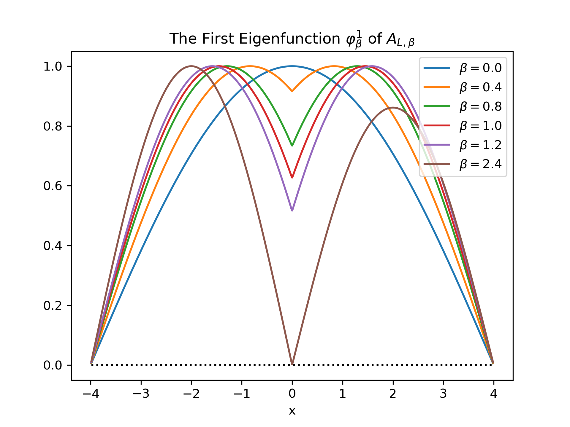
Figure 1. The first eigenfunction of $A_{L,\beta}$ as the parameter $\beta$ increases for $L=4$ and $x_{0}=1$.

Next we observe that the operator $A^{\prime}_{L,\beta}$ adjoint to $A_{L,\beta}=A_{L}+\beta\delta_{0}\delta_{x_{0}}^{\top}$ is given by $A_{L}+\beta\delta_{x_{0}}\delta_{0}^{\top}$ as immediately follows from

$$\langle A_{L,\beta}u,v\rangle=a_{L}(u,v)+\beta u(x_{0})v(0)=a_{L}(v,u)+\beta v(0)u(x_{0})=\langle u,A_{L,\beta}^{\prime}v\rangle,\>u,v\in\operatorname{H}^{1}_{L}.$$

These operators share their eigenvalues and, if we denote their eigenfunctions by $\varphi^{k}_{L,\beta}$, for $A_{L,\beta}$, and by $\psi^{k}_{L,\beta}$, for the adjoint operator, we obtain the spectral resolution given by

$$A_{L,\beta}=\sum_{k=1}^{\infty}\mu^{k}_{L,\beta}\big{\langle}\psi^{k}_{L,\beta},\cdot\big{\rangle}\varphi^{k}_{L,\beta},$$

and the associated semigroup is explicitly given by

$$e^{-tA_{L,\beta}} =\sum_{k=1}^{\infty}\exp\bigl{(}-t\mu^{k}_{L,\beta}\bigr{)}\big{\langle}\psi^{k}_{L,\beta},\cdot\big{\rangle}\varphi^{k}_{L,\beta}$$

$$=\exp\bigl{(}-t\mu^{1}_{L,\beta}\bigr{)}\varphi^{1}_{L,\beta}\Big{\{}\big{\langle}\psi^{1}_{L,\beta},\cdot\big{\rangle}+\sum_{k=2}^{\infty}\exp\Bigl{(}-t\bigl{[}\mu^{k}_{L,\beta}-\mu^{1}_{L,\beta}\bigr{]}\Bigr{)}\big{\langle}\psi^{k}_{L,\beta},\cdot\big{\rangle}\frac{\varphi^{k}_{L,\beta}}{\varphi^{1}_{L,\beta}}\Big{\}},$$

where the second equality holds provided $\varphi^{1}_{L,\beta}>0$. Notice that, in that case, the quotients ${\varphi^{k}_{L,\beta}}/{\varphi^{1}_{L,\beta}}$ are well defined up to the boundary thanks to L’Hôpital’s rule and to $\bigl{(}\varphi^{1}_{L,\beta}\bigr{)}^{\prime}(\pm L)\neq 0$. The latter is seen either by using the maximum principle or by direct inspection of the form of the eigenfunctions. Now the first eigenfunction $\psi^{1}_{L,\beta}$ of $A^{\prime}_{L,\beta}$ is also positive for small $\beta$. This can be seen either by a direct computation similar to the one we preformed above for $\varphi^{1}_{L,\beta}$ or by observing that the adjoint operator has the same structure as the original one. It follows that, given any positive initial datum $u_{0}\in\operatorname{H}^{1}_{L}$, or even in $\operatorname{H}^{-1}_{L}$, one necessarily has that $\big{\langle}u_{0},\psi^{1}_{L,\beta}\big{\rangle}>0$ and the corresponding solution will eventually be positive in $(-L,L)$. The actual time at which this happens will depend on $u_{0}$, leading to individual eventual positivity. This positivity holds as long as both $\varphi^{1}_{L,\beta}$ and $\psi_{L,\beta}^{1}$ are positive, which is the case for $\beta<\beta_{+}$ and some $\beta_{+}>0$. Figure 2 depicts the first eigenfunction of $A_{L,\beta}^{\prime}$ for several values of $\beta$. ∎

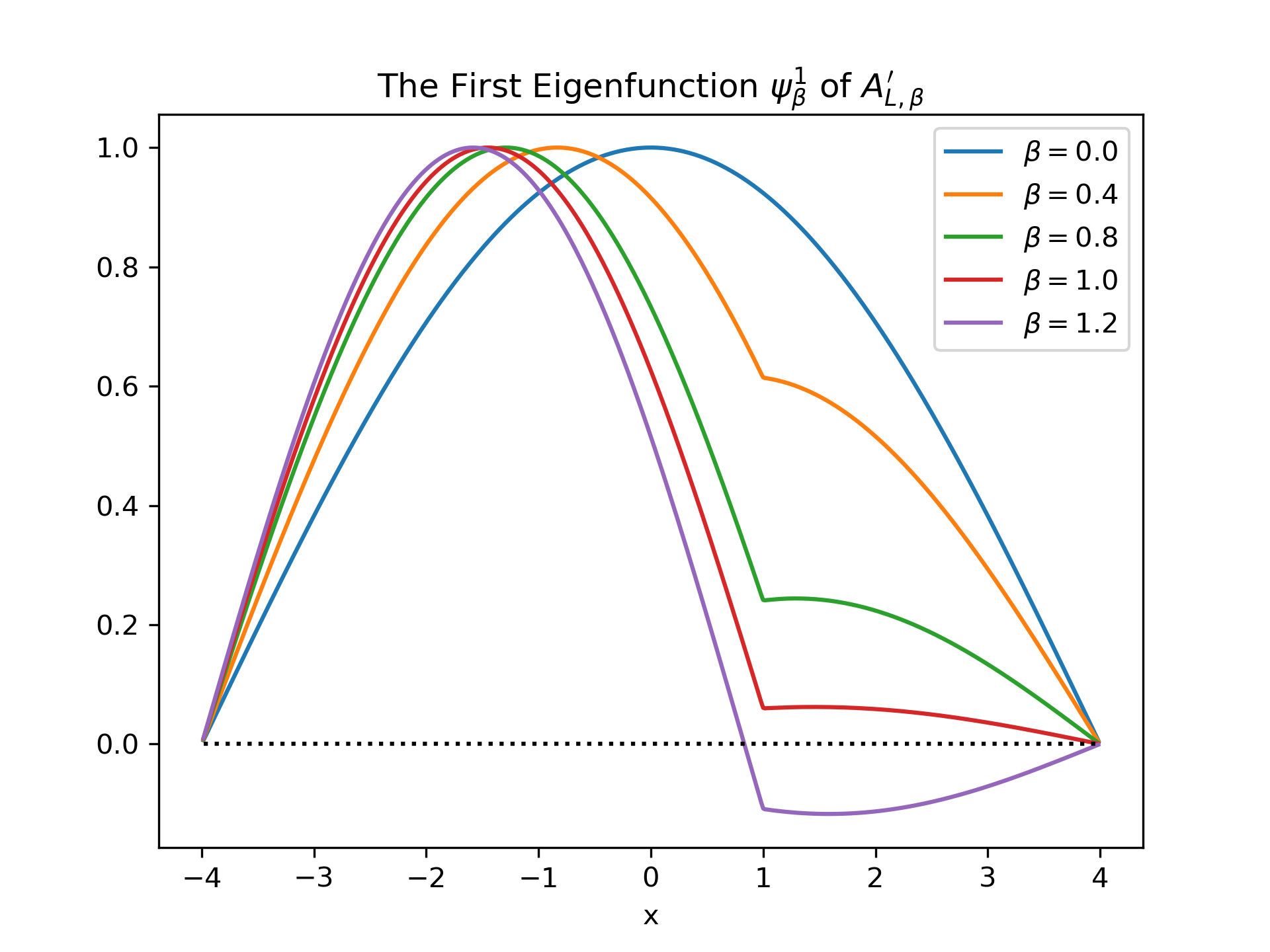
Figure 2. The first eigenfunction of $A_{L,\beta}^{\prime}$ as the parameter $\beta$ increases for $L=4$ and $x_{0}=1$.

Remark 3.2.

Notice that equation (3.9), which determines the eigenvalues of $A_{L,\beta}$ shows that “half” of the eigenvalues, those arising as zeros of $\sin(\lambda L)$, do not in fact depend on $\beta$ at all. In the limit as $L\to\infty$ they contribute to the continuous spectrum of $A_{\beta}$, which we already observed remains unchanged as $\beta$ increases.

The eigenvalues of $A_{L,\beta}$ generated by the zeros of the second factor in (3.9) are partly responsible for the onset of complex spectrum, but mostly contribute to the real spectrum.

Proposition 3.3.

The zeros of the second factor of (3.9) located in $\mathbb{C}\setminus(-\infty,0]$ coincide with those of $1+\beta G^{L}_{s}(x_{0},0)$ appearing in (3.8). For any finite $\beta>0$ and any $L>x_{0}>0$ large enough, there is only a finite number of them and they are close to the zeros of $1+\beta G_{s}(x_{0})$.

Proof.

First notice that the function $\cosh(\lambda L)$ only vanishes for $\lambda=(\frac{\pi}{2L}+\frac{\pi}{L}k)i$, $k\in\mathbb{Z}$. This means that, when looking for zeros of

$$K_{L}(\lambda)=1+\beta\frac{\sinh\bigl{(}\lambda(L-x_{0})\bigr{)}}{2\lambda\cosh(\lambda L)}$$

leading to eigenvalues $\lambda^{2}\in\mathbb{C}\setminus(-\infty,0]$, we can safely consider the equation $J_{L}(\lambda)=0$ instead, where

$$J_{L}(\lambda)=2\cosh(\lambda L)+\beta\frac{\sinh\bigl{(}\lambda(L-x_{0})\bigr{)}}{\lambda}=2\cosh(\lambda L)K_{L}(\lambda),$$

when looking for eigenvalues with non-trivial imaginary part. Zeros of $J_{L}$ in $\mathbb{C}\setminus(-\infty,0]$ therefore account for all and any non-real eigenvalues of $A_{L,\beta}$. We already know that the second factor in (3.9) is the only possible source of non-real eigenvalues of $A_{L,\beta}$, as well. We use the notation

$$H_{L}(\lambda)=2\cos(\lambda L)+\beta\frac{\sin\big{(}\lambda(L-x_{0})\bigr{)}}{\lambda}$$

for that factor. Direct computation shows that, for these functions, it holds that

$$H_{L}(\overline{\lambda})=\overline{H_{L}(\lambda)},\>J_{L}(\overline{\lambda})=\overline{J_{L}(\lambda)},\>\lambda\in\mathbb{C},$$

and that $H_{L}(-\lambda)=H_{L}(\lambda)$, $J_{L}(-\lambda)=J_{L}(\lambda)$. This shows, unsurprisingly, that complex zeros come in complex conjugate pairs. Well-known trigonometric (or hyperbolic) identities show that

$$J_{L}(\lambda)=H_{L}(i\lambda),\>J_{L}(i\lambda)=H_{L}(-\lambda)=H_{L}(\lambda).$$

It follows that

(3.10) $$J_{L}(\alpha+im\alpha)=H_{L}(i\alpha-m\alpha)=\overline{H_{L}(-i\alpha-m\alpha)}=\overline{H_{L}(m\alpha+i\alpha)},\>\alpha\in[0,\infty).$$

Varying $m\in[0,\infty)$ allows for the search of complex zeros on rays emanating from the origin covering the first quadrant (with the exception of the positive imaginary axis), and leads to the determination of all complex eigenvalues in the upper-half plane. In view of the stated properties of the functions of interest, this is sufficient in order to locate all eigenvalues in $\mathbb{C}\setminus(-\infty,0]$. Identity (3.10) readily implies that eigenvalues on $i(0,\infty)$, which are obtained searching for zeros with $m=1$, correspond to the shared zeros of $J_{L}$ and $K_{L}$ on the ray $(1+i)(0,\infty)$. For the other rays in the first quadrant, i.e. for $m\in(0,\infty)\setminus\{1\}$, zeros of $J_{L}$ on $(1,m\,i)(0,\infty)$ correspond to zeros of $H_{L}$ on $(m,i)(0,\infty)$ and vice-versa. We conclude that, while the equations for the zeros of $J_{L}$ and of $H_{L}$ are not equivalent, these two functions have identical zero sets in the open first quadrant.
Next observe that $K_{L}(\lambda)=1+\beta G_{\lambda}^{L}(x_{0},0)$ and that $K_{L}\longrightarrow 1+\beta G_{\lambda}(x_{0})=:K(\lambda)$ as $L\to\infty$, uniformly in subsets which are a positive distance away from $\mathbb{C}\setminus(-\infty,0]$. Uniform convergence holds also for the first derivative of these functions. The zeros with non-trivial imaginary part of the limiting function have been fully characterized in Proposition 2.5. It therefore follows that, for any fixed $\beta>0$ and for $L$ large enough, the zero set of $K_{L}$ in the interior of the first quadrant is close to that of $K$, which was fully understood in Proposition 2.5. This is true due to the fact that these zeros are non-degenerate, a fact that will follow from a later more detailed discussion (see the proof of Proposition 3.5 below). To be more precise, in the limit, the countable simple eigenvalues on the imaginary axis do not accuumulate and are non-degenerate as they are generated by the zeros of the function $z_{\infty}$ appearing in (3.11). As the parameter $\beta$ is dialed back down, these zeros move on smooth curves that do not cross until they reach the real line for $L=\infty$. Due to the uniform convergence mentioned above the same has to remain true away from the real line for any large $L$, as well. ∎

Remark 3.4.

While it is not possible to carry out calculations as explicitly as it was the case for $A_{\beta}$, i.e. for the full line, the fast convergence of the resolvent/kernel as $L\to\infty$ allows one to conclude that the zeros of $1+\beta G_{s}^{L}(x_{0},0)$ located in the interior of the first quadrant are very close to those of $1+\beta G_{s}(x_{0},0)$ already for modest values of $L$ (even for $L=2$ and $x_{0}=1$). In particular, the complex eigenvalues of $A_{L,\beta}$ (situated outside a neighborhood of the origin, and they all are) do behave in a manner very close to those of $A_{\beta}$. The eigenvalues on the negative real axis essentially only contribute to the continuous spectrum in the limit. This is even true for discretizations of $A_{L,\beta}$ for the first few crossings, which can be captured with relatively few grid points. We refer to Figure 4 for a plot of the curve traced by the first pair of complex conjugate eigenvalues parametrized by $\beta$ from the moment they leave the real line (for $L=4,8,16$ and $x_{0}=1$) and to the last section for details about the numerical discretization used in the computations. Notice that the imaginary axis is crossed at $\beta\simeq 70\simeq\beta_{1}$, regardless of the value of $L$.

Proposition 3.5.

For $L$ large enough, there are critical values $\beta_{0,L}>0$ and $\beta_{1,L}>\beta_{0,L}$, so that at $\beta_{0,L}>0$ genuinely complex eigenvalues appear in the spectrum of $A_{\beta,L}$ and so that at $\beta_{1,L}$ a complex conjugate eigenvalue pair crosses the imaginary axis.

Proof.

This follows again from the uniform convergence of corresponding functions determining the non-real eigenvalues of $A_{L,\beta}$ and the complete knowledge of the limiting case $L=\infty$. ∎

Remark 3.6.

The parameter value at which pairs of real eigenvalues merge and become complex conjugate with non-trivial imaginary part appears to have a non-straightfoward relation to the parameter $L$. As for the parameter $\beta_{1,L}$, more can be said analyzing the equation $1+\beta G^{L}_{s}(x_{0},0)$ more closely. To shorten the formulæ, we use the notation $\operatorname{c}$, $\operatorname{s}$, $\operatorname{ch}$, $\operatorname{sh}$, and $\operatorname{th}$ for the functions $\cos$, $\sin$, $\cosh$, $\sinh$, and $\tanh$, respectively. Morever $L_{0}$ will denote $L-x_{0}$. As observed earlier, looking for eigenvalues on the imaginary axis amounts to looking for zeros of the form $\sqrt{s}=\lambda=\alpha+i\alpha$, $\alpha>0$. Decomposing the function $G^{L}_{s}(x_{0},0)=\frac{\operatorname{sh}(L_{0}\lambda)}{2\lambda\operatorname{ch}(L\lambda)}$ into real and complex parts yields

$$\operatorname{Re}\bigl{(}G^{L}_{s}(x_{0},0)\bigr{)}=\frac{1}{4\alpha}\frac{e^{-\alpha}+e^{(1-2L)\alpha}}{1+e^{-2L\alpha}}\frac{1}{\operatorname{c}^{2}(L\alpha)+\operatorname{th}^{2}(L\alpha)\operatorname{s}^{2}(L\alpha)}\cdot\\ \Big{\{}\operatorname{c}(L\alpha)\operatorname{th}(L_{0}\alpha)\operatorname{c}(L_{0}\alpha)+\operatorname{s}(L_{0}\alpha)\operatorname{c}(L\alpha)+\operatorname{s}(L_{0}\alpha)\operatorname{th}(L\alpha)\operatorname{s}(L\alpha)-\operatorname{th}(L_{0}\alpha)\operatorname{c}(L_{0}\alpha)\operatorname{s}(L\alpha)\operatorname{th}(L\alpha)\Big{\}},$$

and

$$\operatorname{Im}\bigl{(}G^{L}_{s}(x_{0},0)\bigr{)}=\frac{1}{4\alpha}\frac{e^{-\alpha}+e^{(1-2L)\alpha}}{1+e^{-2L\alpha}}\frac{1}{\operatorname{c}^{2}(L\alpha)+\operatorname{th}^{2}(L\alpha)\operatorname{s}^{2}(L\alpha)}\cdot\\ \Big{\{}\operatorname{s}(L_{0}\alpha)\operatorname{c}(L\alpha)-\operatorname{c}(L_{0}\alpha)\operatorname{th}(L_{0}\alpha)\operatorname{c}(L\alpha)-\operatorname{th}(L_{0}\alpha)\operatorname{c}(L_{0}\alpha)\operatorname{s}(L\alpha)\operatorname{th}(L\alpha)-\operatorname{s}(L_{0}\alpha)\operatorname{th}(L\alpha)\operatorname{s}(L\alpha)\Big{\}}.$$

Since the term $\operatorname{c}^{2}(L\alpha)+\operatorname{th}^{2}(L\alpha)\operatorname{s}^{2}(L\alpha)$ never vanishes as follows from the fact that it takes the value 1 in $\alpha=0$ and that zeros would otherwise ($\alpha\neq 0$) satisfy $\tanh^{2}(L\alpha)=-\cot^{2}(L\alpha)$, the imaginary part of $1+\beta G^{L}_{s}(x_{0},0)$ can only vanish if the term in the curly brackets vanishes, equivalently iff

$$z_{L}(\alpha)=\operatorname{s}(L_{0}\alpha)\bigl{[}\operatorname{c}(L\alpha)-\operatorname{th}(L\alpha)\operatorname{s}(L\alpha)\bigr{]}-\operatorname{th}(L_{0}\alpha)\operatorname{c}(L_{0}\alpha)\bigl{[}\operatorname{s}(L\alpha)+\operatorname{th}(L\alpha)\operatorname{s}(L\alpha)\bigr{]}=0.$$

Now, for $\alpha\geq\alpha_{0}>0$ and $L>>1$, using the trigonometric addition formulæ to expand the terms with argument $L_{0}=L-x_{0}$ and observing that $\tanh(L_{0}\alpha)\simeq 1\simeq\tanh(L\alpha)$ in this regime, it can be verified that

(3.11) $$z_{L}(\alpha)\simeq-\cos(\alpha x_{0})-\sin(\alpha x_{0})=z_{\infty}(\alpha).$$

The convergence is quite fast as can be seen in Figure 3. For the first zero of interest, the curves are almost identical even for small $L$, and even more so for subsequent zeros. Once the zeros of the imaginary part are known (the first one is the one we care about), the corresponding value of $\beta$ can be recovered by setting

$$\operatorname{Re}\bigl{(}1+\beta G^{L}_{s}(x_{0},0)\bigr{)}=0,$$

and solving for $\beta$. A similar asymptotic analysis of the behavior of the real part of $G^{L}_{s}(x_{0},0)$ as that performed for the imaginary part, reveals that

$$\operatorname{Re}\bigl{(}G^{L}_{s}(x_{0},0)\bigr{)}\simeq\frac{e^{-\alpha}}{4\alpha}\bigl{[}\cos(\alpha x_{0})-\sin(\alpha x_{0})\bigr{]}\text{ for }L\simeq\infty.$$

Again the convergence is very fast and the above approximation delivers a good estimate of the critical value for moderately sized $L$. It is interesting to observe that $\beta_{1,L}$ does not exhibit monotone behavior in $L$, see Figure 3.

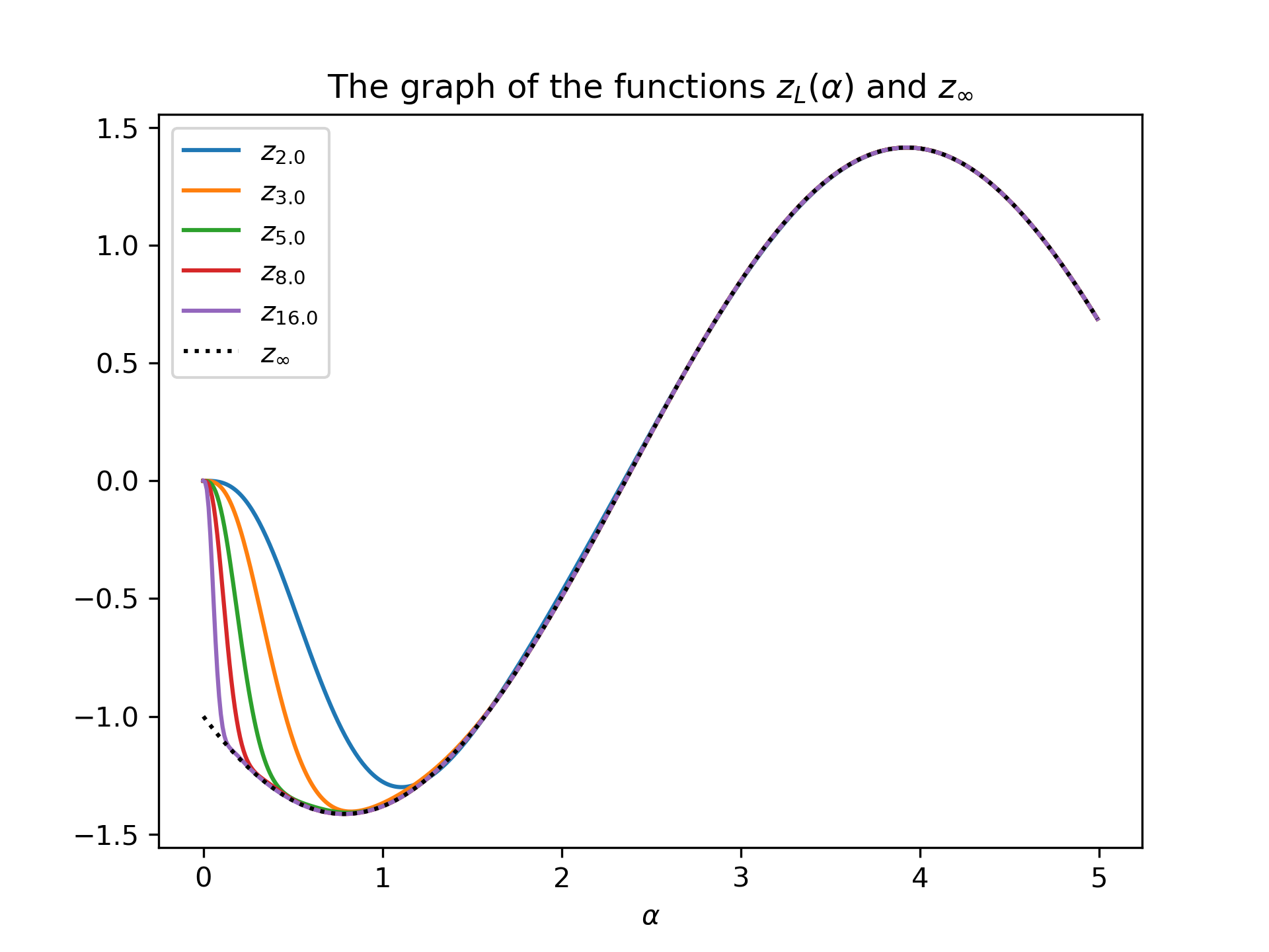
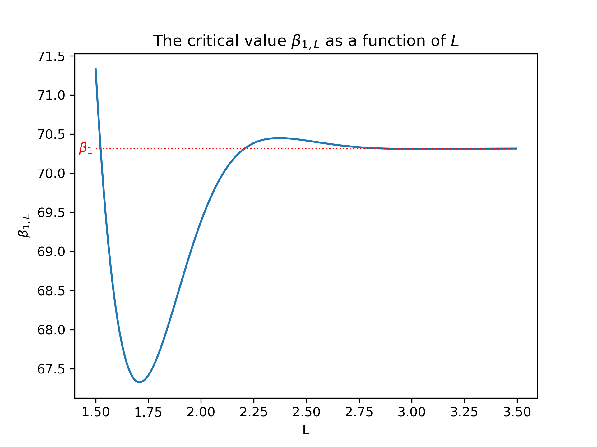
Figure 3. The behavior of the function $z_{L}(\alpha)$ as $L$ grows for $x_{0}=1$.

Remark 3.7.

The behavior of the real spectrum for $L<\infty$ as a function of $L$ is harder to pinpoint analytically. “Half” the eigenvalues do not depend on $\beta$ and just “fill” the negative real axis in the limit as $L\to\infty$. As for the other half, an increasingly small fraction (as $L$ increases) of them merge and become complex as $\beta$ gets larger. This we know since only a finite number of non-real simple eigenvalues appears with increasing $\beta$ (and for large $L$). A numerical calculation of the zeros of the second term in the explicit equation (3.9) confirms this theoretical prediction and can be seen in Figure 5.

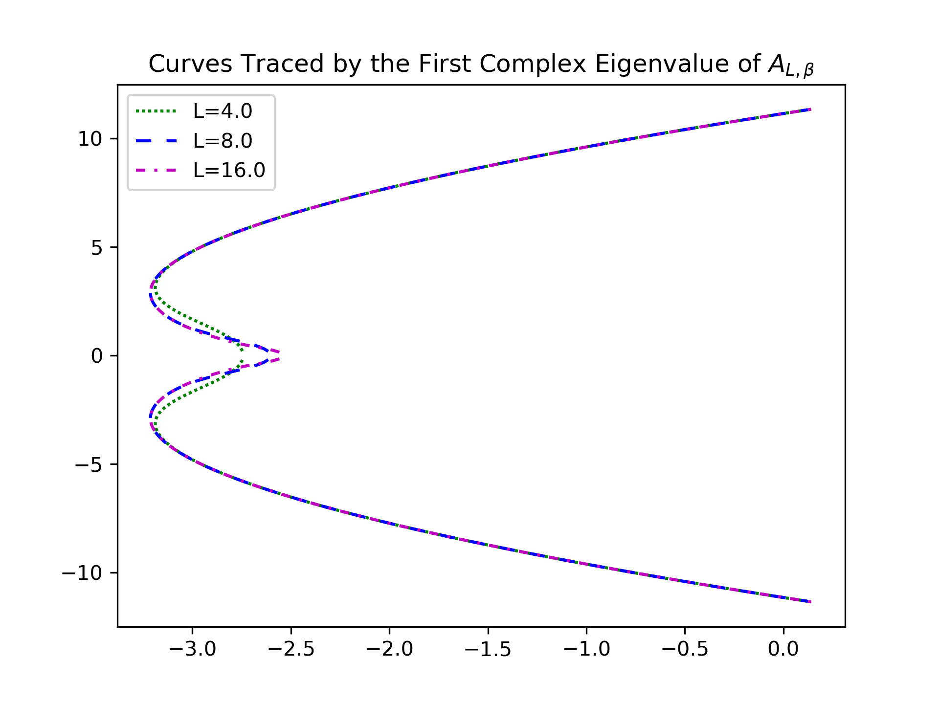
Figure 4. The curve traced by the first pair of complex eigenvalues of $A_{\beta}^{L}$ for interval half-lenghts $L=4,8,16$ and $\beta\in[3.0,73.0)$.

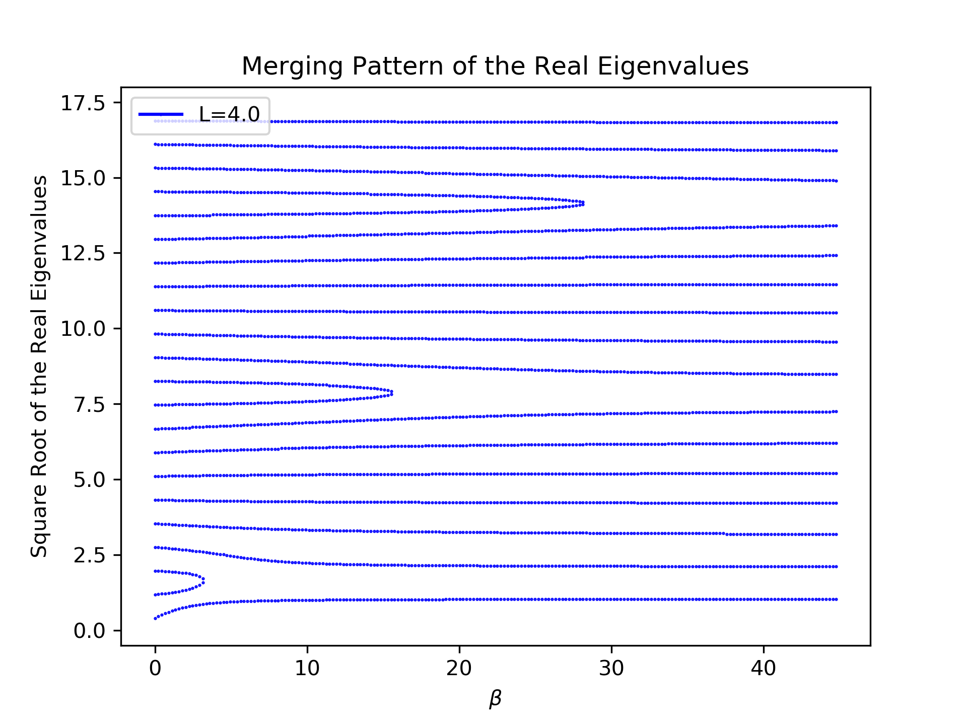
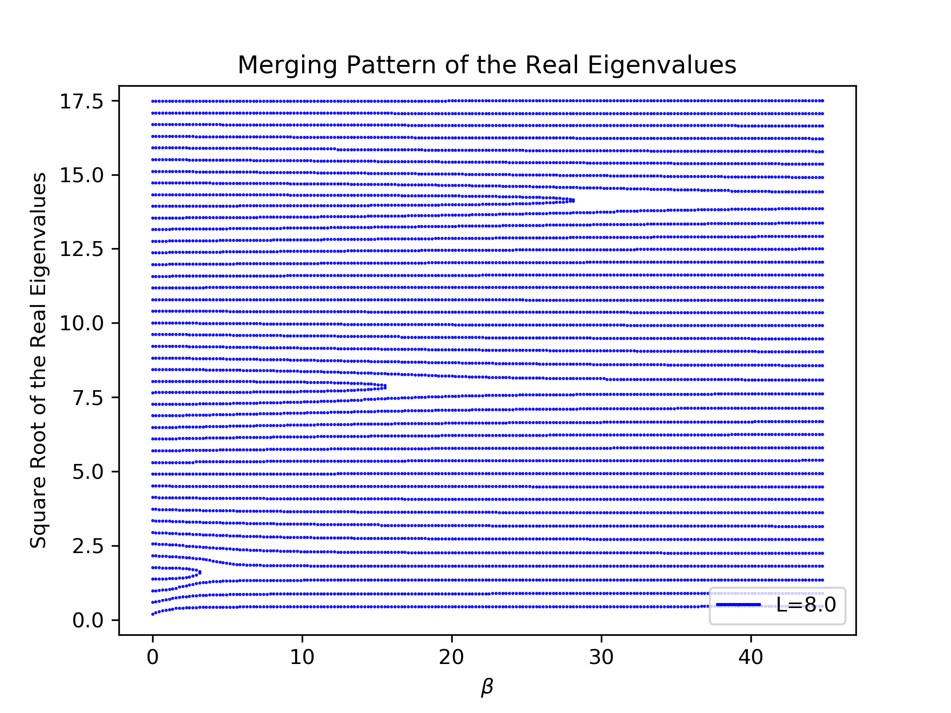
Figure 5. The merging pattern of “half” of the real eigenvalues of $A_{\beta,L}$ observed when $\beta$ is increased for different values of $L$: left $L=4$, right $L=8$.

4. The Nonlinear Equation

Using the analytic semigroup generated by $A$ on $\operatorname{H}^{-1}$, solutions of the nonlinear equation (1.2) can be looked for as fixed points of the equation

(4.1) $$u(t)=e^{-tA}u_{0}-\int_{0}^{t}f\bigl{(}\beta u(t,x_{0})\bigr{)}e^{-(t-\tau)A}\delta_{0}\,d\tau.$$

We consider $u_{0}\in\operatorname{H}^{1}$ and look for a solution $u\in\operatorname{C}\bigl{(}[0,\infty),\operatorname{H}^{1}\bigr{)}$. Evaluating at $x=x_{0}$ yields the Volterra integral equation

$$u(t,x_{0}) =\frac{1}{\sqrt{4\pi t}}\int e^{-\frac{|x_{0}-y|^{2}}{4t}}u_{0}(y)\,dy-\int_{0}^{t}f\bigl{(}\beta u(\tau,x_{0})\bigr{)}\frac{1}{\sqrt{4\pi(t-\tau)}}e^{-x_{0}^{2}/4(t-\tau)}\,d\tau$$

(4.2) $$=:g_{\infty}(t,x_{0})-\int_{0}^{t}f\bigl{(}\beta u(\tau,x_{0})\bigr{)}k_{\infty}(t-\tau,x_{0})\,d\tau.$$

An analogous equation can be obtained for the solution of the nonlinear problem on the interval $[-L,L]$ for $L>x_{0}$ simply replacing the forcing function $g_{\infty}$ and the kernel $k_{\infty}$ with

(4.3) $$g_{L}(t,x_{0})=\bigl{(}e^{-tA_{L}}u_{0}\bigr{)}(x_{0})\text{ and }k_{L}(t,x_{0}),$$

respectively, where $k_{L}$ was defined in (3.5). The main difference between these two kernels is that $k_{L}\in\operatorname{L}^{1}\bigl{(}[0,\infty)\bigr{)}$, due to the exponential decay of the semigroup while $k$ only decays like $1/\sqrt{t}$ for large $t$ and initial data in $\operatorname{H}^{1}$. We will denote by (1.2)_L the corresponding nonlinear equation on the interval $[-L,L]$ with homogeneous Dirichlet boundary condition with the same nonlinearity $f$ and initial condition in $\operatorname{H}^{1}_{L}$. To simplify the combined treatment of the Dirichlet problem on $[-L,L]$ and the problem on the line we will stipulate again that $\operatorname{H}^{1}_{L}=\operatorname{H}^{1}$ for $L=\infty$. Existence and uniqueness are a straightforward application of classical results about nonlinear Volterra integral equations.

Proposition 4.1.

Let $L\in(x_{0},\infty]$ and $u_{0}\in\operatorname{H}^{1}_{L}$ be given. Then
(i) The Volterra integral equation with forcing term $g_{L}$ and kernel $k_{L}(\cdot,x_{0})$ with $L\in(x_{0},\infty)$ has a unique global solution.
(ii) The initial value problem (1.2)_L has a unique global solution $u\in\operatorname{C}\bigl{(}[0,\infty),\operatorname{H}^{1}_{L}\bigr{)}\subset\operatorname{C}\bigl{(}[0,\infty),\operatorname{H}^{1}\bigr{)}$ to any given $u_{0}\in\operatorname{H}^{1}_{L}$ and, therefore, generates a global continuous semiflow on $\operatorname{H}^{1}_{L}$.

Proof.

(i) First notice that $g_{L}(t,\cdot)=e^{-tA_{L}}u_{0}$ is continuous with values in $\operatorname{H}^{1}$ for all $L$ in the given range since $\operatorname{H}^{1}_{L}\hookrightarrow\operatorname{H}^{1}$ for any $L$ by simply extending functions trivially. Since $\operatorname{H}^{1}\hookrightarrow\operatorname{C}$, it follows that $g_{L}(\cdot,x_{0})\in\operatorname{C}\bigl{(}[0,\infty)\bigr{)}$, and, in view of the decay properties of the semigroups, $\lim_{t\to\infty}g_{L}(t,x_{0})=0$. As we are keeping $x_{0}$ fixed in this argument, we remove it from the notation from now on. Existence is obtained by the standard iterative procedure starting with $y_{0}=g_{L}(t)$ and recursively defining

$$y_{n}(t)=g_{L}(t)-\int_{0}^{t}f\bigl{(}\beta y_{n-1}(\tau)\bigr{)}k_{L}(t-\tau)\,d\tau.$$

Setting $\varphi_{n}=y_{n}-y_{n-1}$ and $\varphi_{0}=g_{L}$, we can write $y_{n}=\sum_{k=0}^{n}\varphi_{k}$ and a simple use of the global Lipschitz continuity of the nonlinearity $f$ yields

$$\big{|}\varphi_{n}(t)\big{|}\leq C\int_{0}^{t}\big{|}\varphi_{n-1}(\tau)\big{|}\,d\tau\leq\cdots\leq\|g_{L}\|_{\infty,[0,T]}\frac{(CT)^{n}}{n!},\>t\in[0,T].$$

It follows that $y(\cdot)=\sum_{k=0}^{\infty}\varphi_{k}$ exists and is continuous on $[0,T]$ for any $T>0$. Writing

$$y=y_{n}+\sum_{k=n+1}^{\infty}\varphi_{k}=:y_{n}+\Delta_{n},$$

it is easily seen that

$$y_{n}(t)=y(t)-\Delta_{n}(t)=g_{L}-\int_{0}^{t}k_{L}(t-\tau)f\Bigl{(}\beta\bigl{[}y(\tau)-\Delta_{n}(\tau)\bigr{]}\Bigr{)},$$

from which one obtains that

$$\Big{|}y(t)-g_{L}(t)+\int_{0}^{t}k_{L}(t-\tau)f\bigl{(}\beta y(\tau)\bigr{)}\,d\tau\Big{|} \leq\big{|}\Delta_{n}(t)\big{|}+C\int_{0}^{t}\big{|}\Delta_{n-1}(\tau)\big{|}\,d\tau$$

$$\leq\big{|}\Delta_{n}(t)\big{|}+CT\|\Delta_{n-1}\|_{\infty,[0,T]}.$$

The terms after the last inequality converge to zero uniformly in $t\in[0,T]$ for any fixed $T>0$, showing that $y$ indeed satisfies the Volterra integral equation. Uniqueness follows from similar estimates for the difference of two solutions. We refer to [24, Chapter 4] for missing details.
(ii) Once a solution $y_{L}\in\operatorname{C}\bigl{(}[0,\infty)\bigr{)}$ is known, the right-hand-side of (4.1) is completely determined and the unique mild solution of (1.2) is obtained. It follows from semigroup theory (see e.g. [26, 12]) that the right-hand-side of (4.1) is in $\operatorname{C}\bigl{(}[0,\infty),\operatorname{H}^{1}_{L}\bigr{)}$. The equation (1.2)_L therefore generates a global continuous semiflow on the space $\operatorname{H}^{1}_{L}$ for any $L>x_{0}$. ∎

5. Asymptotic stability for solutions of the nonlinear Volterra integral equation

In this section we will adapt the stability analysis presented in [16, Section 4] that builds on results in [25] to the integral equation obtained from the nonlinear thermostat problem $\eqref{lineTs}_{L}$ with Dirichlet boundary conditions. The nonlinear Volterra integral equation is obtained from the global continous semiflow $\bigl{(}\Phi_{\beta},\operatorname{H}^{1}_{L}\bigr{)}$ induced by $\eqref{lineTs}_{L}$ for arbitrary fixed parameters $L,\beta\in(0,\infty)$ and $x_{0}\in(0,L)\,$. In fact, let $\Phi_{\beta}(\cdot,u_{0})$ be any orbit of the continuous semiflow $\bigl{(}\Phi_{\beta},\operatorname{H}^{1}_{L}\bigr{)}\,$, then

$$u(t):=\Phi_{\beta}(t,u_{0})(x=x_{0})$$

solves the nonlinear, convolution-kernel, Volterra integral equation of the second kind

(5.1) $$y(t)=g_{L}(t)+\int_{0}^{t}a_{L}(t-\tau)f\bigl{(}\beta y(\tau)\bigr{)}\,d\tau\,,\,t>0,$$

where the forcing function $g_{L}\equiv g_{L}(u_{0})$ and the convolution kernel $k_{L}=-a_{L}$ are defined in (4.3) in the discussion at the beginning of the previous section.

Remark 5.1.

In this and the following sections we always assume that the nonlinearity $f:\mathbb{R}\to\mathbb{R}$ has the following properties:

• $f$ is bounded, has a continuous derivative, and is globally Lipschitz continous.

• $f(0)=0$ and $f^{\prime}(0)=1$.

• $f(\beta w)(w-\frac{f(\beta w)}{\beta})>0$ for $w\neq 0\,$ and $\beta\in\mathbb{R}\backslash\{0\}$.

• For the statements on the bifurcation and the stability of periodic solutions we additionally assume that $f\in\operatorname{C}^{\infty}(\mathbb{R},\>\mathbb{R})$.

It may be helpful to think of $f(w)$ as the specific example $\tanh(w)$ that satisfies the above conditions.

The main objective of this section is to prove the following result. Its proof will be given at the end of the section.

Theorem 5.2.

Assume that either

$$L>x_{0}>0\text{ and }\beta\in\bigl{(}0,\hat{\beta}_{1}(x_{0},L)\bigr{)},\text{ for some constant }\hat{\beta}_{1}(x_{0},L)>0$$

or

$$\beta\in\bigl{(}0,\beta_{1}(x_{0})\,\bigr{)}\text{ with }\beta_{1}(x_{0}):=\frac{c_{\pi}}{x_{0}}\,,\,c_{\pi}:=\frac{3\pi}{\sqrt{2}}e^{\frac{3\pi}{4}}\text{ and }L>C(x_{0})\text{ for some constant }C(x_{0})>x_{0}>0$$

holds. Then for arbitrary $u_{0}\in\operatorname{H}^{1}_{L}$ any solution $y\in\operatorname{BC}\bigl{(}(0,\infty),\mathbb{R}\bigr{)}$ of the integral equation (5.1) with parameters $\beta,L,x_{0}$ satisfies $\lim_{t\to\infty}y(t)=0\,$.

The above constants $\hat{\beta}_{1}(x_{0},L)$ and $C(x_{0})$ will be constructed in the proof of the theorem. We proceed by adapting the steps of the proof of the analogous result in [16] to the present situation. First we introduce the following slightly modified auxiliary function.

Definition 5.3.

For $\beta,q\in(0,\infty)$ and $y\in\operatorname{BC}\bigl{(}[0,\infty),\mathbb{R}\bigr{)}$ set

$$W_{\beta,q}(y)(t):=\sum_{i=1}^{2}W_{i}(y)(t),\>t\geq 0,$$

where

$$W_{1}(y)(t) :=\int_{0}^{t}f\bigl{(}\beta y(\tau)\bigr{)}\Bigl{[}y(\tau)-\frac{f\bigl{(}\beta y(\tau)\bigr{)}}{\beta}\Bigr{]}\,d\tau\;,$$

$$W_{2}(y)(t) :=q\,F_{\beta}\bigl{(}y(t)\bigr{)}\text{ for }F_{\beta}(z):=\int_{0}^{z}f(\beta\zeta)\,d\zeta\;.$$

Note that, in the sequel, we will at times suppress the dependence on $\beta$, $q$, and on the function $y$ in the notation and simply write $W$ and $W_{i}$ for $i=1,2$.

The proof of the following lemma is identical to the one given in [16, Lemma 4.3] and is thus omitted.

Lemma 5.4.

Let $\beta,q\in(0,\infty)$ and $y\in\operatorname{BC}\bigl{(}[0,\infty),\mathbb{R}\bigr{)}$. Then

$$W_{i}(t)\geq 0,\>t\geq 0,\>i=1,2.$$

It therefore also holds that $W_{\beta,q}(t)\geq 0$ for $t\geq 0$.

The following decomposition of the auxiliary function W(y)(t) along solutions $y(t)$ of the integral equation (5.1) follows by a simple verification that is carried out in [16, Lemma 4.4] in full detail. We therefore do not reproduce the proof here.

Lemma 5.5.

Fix $L>0,x_{0}\in(0,L)$ and $\beta,q\in(0,\infty)\,$. Let $y\in\operatorname{BC}\bigl{(}(0,\infty),\mathbb{R}\bigr{)}$ be a solution of the integral equation (5.1) with parameters $L,x_{0},\beta$ and $u_{0}\in\operatorname{H}^{1}_{L}\,$. Then

(5.2) $$W_{\beta,q}(t)=V_{\beta,q}(t)+R_{\beta,q}(t),\>t\geq 0\,,$$

where

$$V_{\beta,q}(t):=\int_{0}^{t}f\bigl{(}\beta y(\tau)\bigr{)}\bigl{[}g_{L}(\tau)+qg^{\prime}_{L}(\tau)\bigr{]}\,d\tau+qF_{\beta}\bigl{(}y(0)\bigr{)}$$

and

$$R_{\beta,q}(t)\equiv R_{\beta,q,L}(t):=\int_{0}^{t}f\bigl{(}\beta y(\tau)\bigr{)}\Big{\{}\int_{0}^{\tau}\bigl{[}a_{L}(\tau-\sigma)+q\,a_{L}^{\prime}(\tau-\sigma)\bigr{]}f\bigl{(}\beta y(\sigma)\bigr{)}\,d\sigma-\frac{f\bigl{(}\beta y(\tau)\bigr{)}}{\beta}\Big{\}}\,d\tau.$$

Using convolutions, the last expression can be written more concisely as

$$R_{\beta,q}(t)=\int_{0}^{t}f\bigl{(}\beta y(\tau)\bigr{)}J_{\beta,q}(\tau)\,d\tau,$$

where $J_{\beta,q}$ is defined for $\tau\geq 0$ by

(5.3) $$J_{\beta,q}(\tau):=\Bigl{[}\bigl{[}a_{L}+qa_{L}^{\prime}\bigr{]}*f\bigl{(}\beta y(\cdot)\bigr{)}\Bigr{]}(\tau)-\frac{f\bigl{(}\beta y(\tau)\bigr{)}}{\beta}\,.$$

To apply the Parseval-Plancherel Theorem as in [16, Lemma 4.5] we first collect some properties of the Fourier transform of the kernel $a_{L}(t)$ and of its derivative $a^{\prime}_{L}(t)\,$.

Remarks 5.6.

(a) For $L>0$ and $x_{0}\in(0,L)$ the kernel $a_{L}$ of the Volterra integral equation (5.1) is given by $a_{L}(t)=-k_{L}(t,x_{0})$, i.e. it holds that

(5.4) $$a_{L}(t)=-\frac{1}{L}\sum_{k=0}^{\infty}(-1)^{k}\sin\Bigl{[}\frac{(2k+1)\pi}{2L}(x_{0}+L)\Bigr{]}\,e^{-t\,\lambda^{2}_{2k+1,L}},\>t>0,$$

for $\lambda_{k,L}=\frac{k\pi}{2L}$ according to (3.1),

The kernel $a_{L}$ can be extended to a $\operatorname{C}^{\infty}$-function on $\mathbb{R}$ by setting $a_{L}(t):=0$ for $t\leq 0$. When no confusion seems likely we will not use a different notation for this extension.
Besides the convolution kernel $a_{L}$, the forcing term $g_{L}$ can also be expressed in terms of the basis of eigenfunctions to give

(5.5) $$g_{L}(t)=\sum_{k=1}^{\infty}\langle u_{0},\varphi_{k,L}\rangle\varphi_{k,L}(x_{0})e^{-t\,\lambda^{2}_{k,L}}\;.$$

(b) For $u_{0}\in\operatorname{H}^{1}$ the forcing function $g_{L}$ and its $n$-th derivative are in $\operatorname{BUC}^{\infty}\bigl{(}(0,\infty)\bigr{)}$.
(c) As already observed in (3.5) the Dirichlet heat kernel can be obtained from the heat kernel on the whole real line and can be expressed in terms of the theta function. The (general) theta function $\theta_{1}$ is defined as

$$\theta_{1}(\tau,z):=\sum_{k\in\mathbb{Z}}e^{\pi ik^{2}\tau}\,e^{2\pi ikz}\>,\,\tau,z\in\mathbb{C}\,,\,\operatorname{Im}(\tau)>0,$$

or in less symmetric form by modifying the order of summation

$$\theta_{1}(\tau,z):=2\sum_{k=0}^{\infty}(-1)^{k}q^{(\frac{k+1}{2})^{2}}\,\sin((2k+1)z),\>\tau,z\in\mathbb{C},\>\operatorname{Im}(\tau)>0,\>q:=e^{i\pi\tau}.$$

By setting $\alpha(L,x_{0})=\frac{\pi}{2L}(x_{0}+L)$, it is directly verified from (5.4) and the definition of $\theta_{1}$ that

$$-a_{L}(t)=k_{L}(t,x_{0})=\Bigl{[}e^{-tA_{L}}\delta_{0}\Bigr{]}(x_{0})=\frac{1}{2L}\theta_{1}\Bigl{(}i\frac{4\pi}{L^{2}}t,\alpha(L,x_{0})\Bigr{)}.$$

(d) The kernel $a_{L}(t)$ satisfies

$$\lim_{t\to\infty}a_{L}(t)=0\text{ and }\lim_{t\searrow 0}a(t)=0\>.$$

The limit for $t\to\infty$ is obtained directly from (5.4). To determine the one-sided limit we observe that

$$-a_{L}(t)=\frac{1}{2L}\theta_{1}\Bigl{(}i\frac{4\pi}{L^{2}}t,\alpha(L,x_{0})\Bigr{)},$$

and therefore the limit for ${t\searrow 0}$ follows from known properties of the heat kernel and the theta function.
(e) The kernel $a_{L}(t)$ (extended by 0 for $t\leq 0$) satisfies

$$a_{L}\in\operatorname{BC}^{\infty}(\mathbb{R},\mathbb{R})$$

and its derivatives satisfy

$$a^{(n)}_{L}\in\operatorname{L}^{p}(\mathbb{R}),\>p\in[1,\infty],\>n\geq 1.$$

This again follows from the kernel’s representation (5.4).
(f) The series representation of the Fourier transforms of $a_{L}$ and its derivate $a^{\prime}_{L}$ will be needed in the sequel to recover the Popov stability criterion for the Volterra integral equation. They are given by

(5.6) $$\hat{a}_{L}(\omega)=-\frac{1}{L}\sum_{k=0}^{\infty}(-1)^{k}\frac{\sin\bigl{[}\frac{(2k+1)\pi}{2L}(x_{0}+L)\bigr{]}}{i\omega+\lambda_{2k+1,L}},$$

and by

(5.7) $$\widehat{a^{\prime}_{L}}(\omega)=i\omega\hat{a}_{L}(\omega)=-\frac{i\omega}{L}\sum_{k=0}^{\infty}(-1)^{k}\frac{\sin\bigl{[}\frac{(2k+1)\pi}{2L}(x_{0}+L)\bigr{]}}{i\omega+\lambda_{2k+1,L}},$$

respectively.
This follows from elementary properties of the Fourier transform similarly as discussed in [16, Remarks 2.2 (g)].
(g) The Laplace transform $\mathcal{L}(a_{L})$ of $a_{L}(t)$ is given by

$$\mathcal{L}(a_{L})(s)=-\frac{1}{L}\sum_{k=0}^{\infty}(-1)^{k}\frac{\sin\bigl{[}\frac{(2k+1)\pi}{2L}(x_{0}+L)\bigr{]}}{s+\lambda_{2k+1,L}}$$

for $s\in\big{\{}z\in\mathbb{C}\,\big{|}\,\operatorname{Re}(z)>0\big{\}}$. It also has the explicit representation

(5.8) $$\mathcal{L}(a_{L})(s)=-\frac{\sinh\bigl{(}\sqrt{s}(L-x_{0})\bigr{)}}{2\sqrt{s}\cosh(\sqrt{s}L)}\,.$$

The series representation of the Laplace transform is obtained from (5.4) by elementary integrations. The explicit representation follows from (3.7). A direct verification that the explicit form is represented by the above series is also given in [6] by a partial fraction expansion and by determination of the residuals of the poles of (5.8).
(h) We note that, for given parameters $L>x_{0}>0\,$, the associated transfer function

(5.9) $$G_{L,x_{0}}(s):=-\mathcal{L}(a_{L})(s)=\frac{\sinh\bigl{(}\sqrt{s}(L-x_{0})\bigr{)}}{2\sqrt{s}\cosh(\sqrt{s}L)}\,,$$

can be expressed in terms of the Fourier transforms of $a_{L}$ and that of $a_{L}^{\prime}\,$. In fact, for $\omega\in\mathbb{R}\backslash\{0\}$, it holds that

$$\operatorname{Re}\bigl{(}G_{L,x_{0}}(i\omega)\bigr{)}=-\operatorname{Re}\bigl{(}\hat{a}_{L}(\omega)\bigr{)}$$

and

$$\omega\operatorname{Im}\bigl{(}G_{L,x_{0}}(i\omega)\bigr{)}=\operatorname{Re}\bigl{(}\widehat{a^{\prime}_{L}}(\omega)\bigr{)}.$$

The inequality

(5.10) $$\operatorname{Re}\bigl{(}\hat{a}_{L}(\omega)\bigr{)}+q\operatorname{Re}\bigl{(}\widehat{a^{\prime}_{L}}(\omega)\bigr{)}-\frac{1}{\beta}\leq 0,\>\omega\in\mathbb{R}\backslash\{0\},$$

is then equivalent to

(5.11) $$\operatorname{Re}\bigl{(}G_{L,x_{0}}(i\omega)\bigr{)}-q\omega\operatorname{Im}\bigl{(}G_{L,x_{0}}(i\omega)\bigr{)}\geq-\frac{1}{\beta},\>\omega\in\mathbb{R}\backslash\{0\}.$$

We will use this relationship between $G_{L,x_{0}}(s)$ and $\hat{a}_{L}$ and $\widehat{a^{\prime}_{L}}$ to verify that the stability condition (5.10) (which we will obtain below from the analysis of the integral equation (5.1)) is equivalent to the well-known Popov stability criterion (5.11) when applied to the transfer function $G_{L,x_{0}}$.

In the next lemma we apply the Parseval-Plancherel Theorem to derive an alternative representation of $R_{\beta,q}\,$. It will reveal a condition, expressed in terms of the Fourier transforms of $a_{L}(t)$ and $a^{\prime}_{L}(t)\,$, which implies $R_{\beta,q}(t)\leq 0\;$. The nonnegativity of the quantity $W_{\beta,q}$ will then allow to bound $V_{\beta,q}$ from above. The proof is straightforward and can be found in [16, Lemma 4.5].

Lemma 5.7.

Let $\beta,q,L\in(0,\infty)$ and $x_{0}\in(0,L)\,$. Let $y\in\operatorname{BC}\bigl{(}(0,\infty),\mathbb{R}\bigr{)}$ be a solution of the integral equation (5.1) with parameters $L,x_{0},\beta$ and $u_{0}\in\operatorname{H}^{1}_{L}$. Then

$$R_{\beta,q}(t)=\frac{1}{2\pi}\int_{-\infty}^{\infty}{\hat{f}^{2}_{\beta,\theta_{t}}}(\omega)\bigl{[}\hat{a}_{L}(\omega)+q\,\widehat{a_{L}^{\prime}}(\omega)-\frac{1}{\beta}\bigr{]}\,d\omega,\>t\geq 0,$$

where

$$f_{\beta,\theta_{t}}(\tau):=f\bigl{(}\beta y(\tau)\bigr{)}\theta_{t}(\tau),\>\tau\in\mathbb{R},\>t\geq 0,$$

with

$$\theta_{t}(\tau):=\begin{cases}1,&\tau\in[0,t],\\ 0,&\tau\in\mathbb{R}\setminus[0,t]\end{cases}$$

and $y(\tau):=0$ for $\tau<0\,$.

The Fourier transforms of $a_{L}$ and $a_{L}^{\prime}$ were discussed in Remarks 5.6. Since $f_{\beta,\theta_{t}}\in\operatorname{L}^{1}(\mathbb{R})\cap\operatorname{L}^{2}(\mathbb{R})$ for each $t\geq 0\,$, its Fourier transform is defined classically.

After these clarifications we can formulate a lemma showing that controlling the sign of $R_{\beta,q,L}(t)$ for $t\geq 0$ leads to a bound for $V_{\beta,q,L}(t)$. The proof of this lemma is simpler than its counterpart in [16, Lemma 4.10] for the case of Neumann boundary conditions and boundary control. This is due to the fact that the semigroup associated with the heat equation on $(-L,L)$ subject to Dirichlet boundary conditions decays to the trivial solution exponentially for any initial state $u_{0}\in H^{1}_{L}$.

Lemma 5.8.

Let $\beta,L\in(0,\infty)$ and $x_{0}\in(0,L)\,$. Let $y\in\operatorname{BC}\bigl{(}(0,\infty),\mathbb{R}\bigr{)}$ be a solution of the integral equation (5.1) with parameters $L,x_{0},\beta$ and $u_{0}\in\operatorname{H}^{1}_{L}$. Then, if for some $q>0$ it holds that

$$R_{\beta,q,L}(t)\leq 0\text{ for }t\geq 0,$$

then the function $V(t)\equiv V_{\beta,q,L}(t)$ defined in Lemma 5.5 satisfies

$$0\leq V(t)\leq c,\>t\geq 0,$$

for a constant $c>0$ independent of $t\geq 0$.

Proof.

As $R(t)\leq 0$ and by the definition of $V$ and $W\,$, it holds that

$$0\leq V(t)=\int_{0}^{t}f\bigl{(}\beta y(\tau)\bigr{)}\bigl{[}g_{L}(\tau)+q\,g^{\prime}_{L}(\tau)\bigr{]}\,d\tau+W_{2}(y)(0),\>t\geq 0,$$

and therefore

$$V(t)\leq\int_{0}^{t}\big{|}f\bigl{(}\beta y(\tau)\bigr{)}\big{|}\,\big{|}g_{L}(\tau)\big{|}d\tau+q\int_{0}^{t}\big{|}f\bigl{(}\beta y(\tau)\bigr{)}\big{|}\,\big{|}g^{\prime}_{L}(\tau)\big{|}\,d\tau+W_{2}(y)(0),\>t\geq 0\,.$$

The assertion now follows from the assumed boundedness of $f(\beta\cdot)$ and from the exponential decay and analyticity of the semigroup $e^{-tA_{L}}$ associated with the heat equation on $(-L,L)$ subject to Dirichlet boundary conditions. Namely, in order to bound $V(t)$ by a constant independent of $t$ we use the estimate

$$\big{|}g_{L}(\tau)\big{|}=\big{|}\bigl{(}e^{-\tau A_{L}}u_{0}\bigr{)}(x_{0})\big{|}\leq c\|e^{-\tau A_{L}}u_{0}\|_{\operatorname{H}^{1}_{L}}\leq c\,e^{-\alpha_{L}\tau}\|u_{0}\|_{\operatorname{H}^{1}_{L}}\>,$$

and the estimate

$$\big{|}g^{\prime}_{L}(\tau)\big{|}=\big{|}\bigl{(}A_{L}e^{-\tau A_{L}}u_{0}\bigr{)}(x_{0})\big{|}\leq c\|e^{-\tau A_{L}}A_{L}u_{0}\|_{\operatorname{H}^{\frac{1}{2}+\varepsilon}_{L}}\leq\frac{c}{\tau^{\frac{3}{4}+\frac{\varepsilon}{2}}}e^{-\alpha_{L}\tau}\|A_{L}u_{0}\|_{\operatorname{H}^{-1}_{L}}\>,$$

which are valid for $\tau>0$, $\varepsilon\in(0,\frac{1}{2})$ and by the choice of an appropriate constant $\alpha_{L}>0\,$. We refer to [12] or [26] for these standard estimates on analytic semigroups in interpolation spaces.

∎

Next we verify that bounded and continuous solutions of the Volterra integral equation (5.1) are also uniformly continuous. As for the previous lemma, the proof turns out to be simpler than its counterpart [16, Lemma 4.11] in the case of Neumann boundary conditions.

Proposition 5.9.

Let $\beta,L\in(0,\infty)$ and $x_{0}\in(0,L)\,$. Let $y\in\operatorname{BC}\bigl{(}(0,\infty),\mathbb{R}\bigr{)}$ be a solution of the integral equation (5.1) with parameters $L,x_{0},\beta$ and $u_{0}\in\operatorname{H}^{1}_{L}$. Then $y\in\operatorname{BUC}\bigl{(}(0,\infty),\mathbb{R})\bigr{)}$.

Proof.

Since $y$ solves (5.1), we have that

$$y(t)=g_{L}(t)+\int_{0}^{t}a_{L}(t-\tau)f\bigl{(}\beta y(\tau)\bigr{)}\,d\tau,\>t\geq 0,$$

where $g_{L}(t)=\bigl{(}e^{-tA_{L}}u_{0}\bigr{)}(x_{0})$ is the forcing function induced by $u_{0}$. It suffices to verify that both terms in the above sum are uniformly continuous. Uniform continuity of the first term holds on any finite interval and the derivative of $y$ is bounded for $t\geq 1$ by the standard smoothing effect of analytic semigroups. Hence $g_{L}$ is uniformly continuous on $(0,\infty)\,$.
The second term can be written as a convolution

$$\int_{0}^{t}a_{L}(t-\tau)f\bigl{(}\beta y(\tau)\bigr{)}\,d\tau=\Bigl{[}a_{L}*\bigl{(}f\circ(\beta y)\bigr{)}\Bigr{]}(t),\>t\geq 0.$$

Since $a_{L}\in\operatorname{L}^{1}\bigl{(}[0,\infty)\bigr{)}$ and $f\circ(\beta y)\in\operatorname{L}^{\infty}\bigl{(}[0,\infty)\bigr{)}$ by the assumed boundedness of $f$, well-known results on the regularity properties of convolutions imply the uniform continuity of the second term (see e.g. [3] or [11]). ∎

We will now show the following statement: if, for a given fixed choice of the parameters $\beta,L,x_{0}$ and $u_{0}\in\operatorname{H}^{1}_{L}$, a constant $q>0$ can be determined, such that $R_{\beta,q,L}(t)\leq 0$ along the solution $y(t)$ of (5.1), then this implies the convergence of $y(t)$ to zero.
By Lemma 5.7 a suitable constant $q>0$ is found if it verifies the inequality

$$\hat{a}_{L}(\omega)+q\,\widehat{a_{L}^{\prime}}(\omega)-\frac{1}{\beta}\leq 0\text{ for }\omega\in\mathbb{R}\backslash\{0\}.$$

If such a $q>0$ can be found, then it does not depend on the initial state $u_{0}\in\operatorname{H}^{1}_{L}\,$, since $u_{0}$ does not appear in the above inequality. However, the choice of such a suitable $q>0$ may and does depend on the choice of the parameters $\beta,L,x_{0}$, as will be discussed below. By the relationship between the transfer function $G_{L}(s)$ and the Fourier transform of the kernel $a_{L}(t)$ discussed in Remarks 5.6 the search of $q$ can be reinterpreted as the task of finding a straight line in the complex plane with positive slope $\frac{1}{q}$ that intersects the real axis at $-\frac{1}{\beta}$ such that the so-called Popov curve associated with the kernel $a_{L}$ lies to the right of that straight line. We refer to [16, Section 3] for a sketch of this relationship to feedback control problems and the celebrated Popov criterion. The following proposition is a slight adaptation of the proof of [16, Proposition 4.1].

Proposition 5.10.

Fix $\beta,L\in(0,\infty)$ and $x_{0}\in(0,L)\,$. Let $y\in\operatorname{BC}\bigl{(}(0,\infty),\mathbb{R}\bigr{)}$ be a solution of the integral equation (5.1) with parameters $L,x_{0},\beta$ and $u_{0}\in\operatorname{H}^{1}_{L}$. If for some $q>0$ it holds that

$$R_{\beta,q,L}(t)\leq 0\text{ for }t\geq 0,$$

then

$$\lim_{t\to\infty}y(t)=0.$$

Proof.

By assumption there exists $q>0$ such that

$$R_{\beta,q,L}(t)\leq 0\text{ for }t\geq 0.$$

By Lemma 5.8 ther exists $c>0$ such that

$$c\geq V_{\beta,q,L}(t)\geq W_{\beta,q}(t)\geq W_{1,\beta}(t)\geq 0,$$

for $t\geq 0$, i.e. such that

$$W_{1,\beta}(t)=\int_{0}^{t}f\bigl{(}\beta y(\tau)\bigr{)}\bigl{[}y(\tau)-\frac{f\bigl{(}\beta y(\tau)\bigr{)}}{\beta}\bigr{]}\,d\tau=:\int_{0}^{t}H\bigl{(}y(\tau)\bigr{)}\,d\tau\leq c<\infty,$$

for $t\geq 0$. As shown in [16, Lemma 4.12] the function $H(y)$ is non-negative, only vanishes if $y=0$, and is uniformly continuous. Assume next by contradiction that $y(t)\not\to 0$ as $t\to\infty$. Then, since $H(\xi)>0$ for $0\neq\xi\in\mathbb{R}$, there is a sequence $(t_{m})_{m\in\mathbb{N}}$ in $\mathbb{R}$ with $t_{m}\to\infty$ and a constant $\varepsilon>0$ such that

$$H\bigl{(}y(t_{m})\bigr{)}\geq 2\varepsilon\text{ for all }m\in\mathbb{N}.$$

Since $H\circ y\in\operatorname{BUC}\bigl{(}[0,\infty)\bigr{)}$, a $\delta>0$ can be found such that

$$H\bigl{(}y(t)\bigr{)}\geq c\text{ for }t\in[t_{m}-\delta,t_{m}+\delta],$$

and all $m\in\mathbb{N}$. It follows that

$$W_{1}(t_{m})=\int_{0}^{t_{m}}H\bigl{(}y(\tau)\bigr{)}\,d\tau\geq\sum_{k=1}^{m-1}\int_{t_{k}-\delta}^{t_{k}+\delta}H\bigl{(}y(\tau)\bigr{)}\,d\tau\geq(m-1)2\delta\varepsilon,$$

which contradicts the boundedness of $W_{1}$ on $[0,\infty)$ since $m$ can be chosen arbitrarily large. ∎

In order to complete the proof of Theorem 5.2 it remains to show that, for suitably constructed constants $\hat{\beta}_{1}(x_{0},L)>0$ and $C(x_{0})$, either the assumption

$$\beta\in\bigl{(}0,\hat{\beta}_{1}(x_{0},L)\bigr{)}\text{ and arbitrary }L>x_{0}>0,$$

or the assumption

$$\beta\in\bigl{(}0,\beta_{1}(x_{0})\bigr{)}\text{ and }L>C(x_{0})>x_{0}>0,$$

are sufficient to find a $q\equiv q(x_{0},\beta)>0$ such that

$$\hat{a}_{L}(\omega)+q\,\widehat{a_{L}^{\prime}}(\omega)-\frac{1}{\beta}\leq 0\text{ for }\omega\in\mathbb{R}\backslash\{0\}.$$

We note that, by symmetry, it suffices to verify the above inequality for $\omega>0$. The following discussion of the limit of the transfer function $G_{L,x_{0}}(s)$ for large $L$ is an important element of the proof.

Remark 5.11.

Fix $x_{0}>0$ and consider the transfer function $G_{L,x_{0}}(s)$ for $L\in(x_{0},\infty)$. Then

(5.12) $$G_{L,x_{0}}(s)=\frac{\sinh\bigl{(}\sqrt{s}(L-x_{0})\bigr{)}}{2\sqrt{s}\cosh(\sqrt{s}L)}\to G_{x_{0}}(s)=\frac{e^{-\sqrt{s}\,x_{0}}}{2\sqrt{s}}\text{ as }L\to\infty,$$

uniformly on compact subsets of $\mathbb{C}\backslash(-\infty,0]$. The convergence is also uniform for $s$ in (unbounded) subsets of the imaginary axis of the form $i\,\bigl{(}\mathbb{R}\setminus(-\varepsilon,\varepsilon)\bigr{)}$.

Proof.

Note that by expanding $\sinh(z_{1}+z_{2})$ we obtain

$$G_{L,x_{0}}(s)\,=\,\frac{1}{2\sqrt{s}}\bigl{[}\cosh(\sqrt{s}x_{0})\,\tanh(\sqrt{s}L)-\sinh(\sqrt{s}x_{0})\bigr{]}.$$

Also note that whenever $\operatorname{Re}(\sqrt{s})>0\Leftrightarrow s\in\mathbb{C}\backslash(-\infty,0]$ it holds that

$$\lim\limits_{L\to\infty}\tanh(\sqrt{s}L)=1,$$

and the convergence is uniform on compact subsets of $\mathbb{C}\backslash(-\infty,0]$. Since $\frac{1}{\sqrt{s}}$ is bounded on such subsets and $\cosh(\sqrt{s}x_{0})-\sinh(\sqrt{s}x_{0})=e^{-\sqrt{s}\,x_{0}}$ the first assertion follows. Observe that we write $\sqrt{z}$ for the principal branch of the complex square root. Hence $\sqrt{\pm i}=\frac{1}{\sqrt{2}}(1\pm i)$ and $\operatorname{Re}(\sqrt{\pm i})=\frac{1}{\sqrt{2}}>0$. Therefore $\tanh(\sqrt{i\omega}L)$ converges to 1 as $L\to\infty$ uniformly for $\omega$ over any set of the form $\mathbb{R}\setminus(-\varepsilon,\varepsilon)$. Since $\frac{1}{\sqrt{s}}$ is bounded on sets of that form the second assertion follows. ∎

In analogy to [16, Proposition 4.2.] we introduce the Popov set corresponding to a given transfer function. The set contains the frequencies $\omega$ at which the Popov curve in the complex plane

$$\operatorname{Re}[G_{x_{0}}(i\omega)]+i\,\omega\,\operatorname{Im}[G_{x_{0}}(i\omega)],\>\omega>0,$$

intersects the imaginary axis. Describing the structure of the Popov set will help finding a parameter range for $\beta$ that guarantees the asymptotic stability of the trivial solution of (1.2) for given parameters $L>x_{0}>0$.

Definition 5.12.

For $L>x_{0}>0$ we set

$$\Omega^{\text{Pop}}_{x_{0}}:=\Big{\{}\omega>0\,\Big{|}\,\operatorname{Im}\Bigl{(}\>\operatorname{Re}[G_{x_{0}}(i\omega)]+i\omega\operatorname{Im}[G_{x_{0}}(i\omega)]\Bigr{)}=0\Big{\}}=\big{\{}\omega>0\,\big{|}\,\operatorname{Im}\bigl{[}G_{x_{0}}(i\omega)\bigr{]}=0\big{\}}$$

and

$$\Omega^{\text{Pop}}_{L,x_{0}}:=\Big{\{}\omega>0\,\Big{|}\,\operatorname{Im}\Bigl{(}\operatorname{Re}[G_{L,x_{0}}(i\omega)]+i\omega\operatorname{Im}[G_{L,x_{0}}(i\omega)]\Bigr{)}=0\Big{\}}=\big{\{}\omega>0\,\big{|}\,\operatorname{Im}\bigl{[}G_{L,x_{0}}(i\omega)\bigr{]}=0\big{\}}.$$

In the next proposition we show that the Popov set of the limiting transfer function $G_{x_{0}}$ can be described explicitly. By determining the first zero $\omega_{1}\approx 11.1033$ of $1+\tan(\sqrt{\frac{\omega}{2}}x_{0})\,$ for the sensor location $x_{0}=1$ we recover the constant $\beta_{1}\approx 70.3134$, found above in (2.5), by using the relationship

(5.13) $$1+\beta_{1}\,G_{L,x_{0}}(i\omega_{1})=0.$$

This relationship between the Popov set and the critical parameter values of $\beta$ is understood by observing that

$$\operatorname{Im}\bigl{[}1+\beta\,G_{L,x_{0}}(i\omega)\bigr{]}=\operatorname{Im}\bigl{[}G_{L,x_{0}}(i\omega)\bigr{]}.$$

This entails that the locations where the imaginary part of (5.13) vanishes are independent of $\beta$. Once the zeros $\omega$ of the imaginary part of the transfer function $G_{L,x_{0}}$ are found, one recovers the corresponding critical values for $\beta$ by simply equating the real part to zero, i.e. by solving

$$\operatorname{Re}\bigl{[}1+\beta\,G_{L,x_{0}}(i\omega)\bigr{]}=0,$$

for $\beta$. The smallest positive solution arising in the above procedure is precisely $\beta_{1}$. This relationship between the Popov set $\Omega^{\text{Pop}}_{x_{0}}$ and the corresponding parameter values for $\beta$ that correspond to the existence of a pair of complex conjugate eigenvalues of the operator $-A_{\beta}$ lying on the imaginary axis is also discussed in more detail in the remarks following [16, Proposition 4.9].

Proposition 5.13.

For $x_{0}>0$, the Popov set of $G_{x_{0}}$ is given as the solution set

(5.14) $$\Omega^{\text{Pop}}_{x_{0}}=\big{\{}\omega>0\,\big{|}\,1+\tan\bigl{(}x_{0}\sqrt{\omega/2}\bigr{)}=0\big{\}}=\big{\{}\omega_{k}=\frac{(4k-1)^{2}\pi^{2}}{8x_{0}^{2}}\,\big{|}\,k=1,2,3,\dots\big{\}}.$$

Hence $\Omega^{\text{Pop}}_{x_{0}}$ is an infinite countable set that consists of positive, non-degenerate (simple) roots of the function $1+\tan(x_{0}\sqrt{\omega/2})$.

Proof.

Setting $r:=-x_{0}\sqrt{\omega}<0$ we observe that

$$\operatorname{Im}[\,G_{x_{0}}(i\omega)\>\bigr{]}=0\Leftrightarrow\operatorname{Im}[\,\frac{e^{r\,\sqrt{i}}}{\sqrt{i}}\>\bigr{]}=0,$$

and since it holds that $e^{r\sqrt{i}}=e^{r\alpha}\cos(r\alpha)+ie^{r\alpha}\sin(r\alpha)$, with $\alpha:=\sin(\frac{\pi}{4})=\cos(\frac{\pi}{4})=\frac{1}{\sqrt{2}}$, we find that

$$\operatorname{Im}\Bigl{[}\frac{e^{r\sqrt{i}}}{\sqrt{i}}\Bigr{]}=0\Longleftrightarrow\operatorname{Im}\Bigl{[}\overline{\sqrt{i}}\cos(r\alpha)+\sqrt{i}\sin(r\alpha)\Bigr{]}=0\Longleftrightarrow\cos(r\alpha)=\sin(r\alpha),$$

and thus, for $\omega>0$, the assertion

$$\operatorname{Im}[G_{x_{0}}(i\omega)\>\bigr{]}=0\,\Longleftrightarrow 1+\tan\bigl{(}x_{0}\sqrt{\omega/2}\bigr{)}=0$$

follows. The other statements follow from elementary properties of $\tan(x)\,$. ∎

We note that the Popov set $\Omega^{\text{Pop}}_{x_{0}}$ also contains values $\omega_{k}$ that lead to positive values of $G_{x_{0}}(i\omega_{k})$ and thus to negative critical values $\beta(\omega_{k})$. More precisely, if we set

$$\Omega^{\text{Pop}\,+}_{x_{0}}:=\big{\{}\omega\in\Omega^{\text{Pop}}_{x_{0}}\,\big{|}\,G_{x_{0}}(i\omega)<0\big{\}}\text{ and }\Omega^{\text{Pop}\,-}_{x_{0}}:=\big{\{}\omega\in\Omega^{\text{Pop}}_{x_{0}}\,\big{|}\,G_{x_{0}}(i\omega)>0\big{\}},$$

then

$$\Omega^{\text{Pop}\,+}_{x_{0}}=\big{\{}\omega_{k}=\frac{(4k-1)^{2}\pi^{2}}{8x_{0}^{2}}\,\big{|}\,k\in 2\mathbb{N}-1\big{\}}\text{ and }\Omega^{\text{Pop}\,-}_{x_{0}}=\big{\{}\omega_{k}=\frac{(4k-1)^{2}\pi^{2}}{8x_{0}^{2}}\,\big{|}\,k\in 2\mathbb{N}\big{\}},,$$

where $\mathbb{N}:=\{1,2,3,...\}\,$. This is analogous to the discussion in [16] and in Section 3 and also captures that pairs of conjugate complex eigenvalues in the spectrum of $A_{\beta}$ do cross the imaginary axis for certain negative values of $\beta$, which are determined by

$$-\frac{1}{G_{x_{0}}(i\omega)}\text{ for }\omega\in\Omega^{\text{Pop}\,-}_{x_{0}}.$$

The positive values of $\beta$ where a crossing occurs are found by

$$-\frac{1}{G_{x_{0}}(i\omega)}\text{ for }\omega\in\Omega^{\text{Pop}\,+}_{x_{0}}.$$

Thus the Popov set $\Omega^{\text{Pop}}_{x_{0}}=\Omega^{\text{Pop}\,+}_{x_{0}}\,\cup\ \Omega^{\text{Pop}\,-}_{x_{0}}$ captures both the positive and negative values of $\beta$ where complex conjugate eigenvalue pairs of $A_{\beta}$ cross the imaginary axis. By the positivity of the semigroup for $\beta\leq 0$ the stability of the trivial solution is determined by the (real) principal eigenvalue and not by a Hopf bifurcation induced by a complex conjugate pair of eigenvalues first crossing into the unstable complex half plane. In that sense, for negative values of $\beta$, the problem has positivity properties that lead to a more familiar behavior which is well-studied in the context of semilinear parabolic equations. We also refer to [15] for a discussion of positivity aspects.

5.1. The Popov criterion in the Limit $L=\infty$

Next we show that the stability criterion (5.11) can be verified for the limiting transfer function $G_{x_{0}}(s)$.

Proposition 5.14.

For any $x_{0}>0$ there exists $\beta_{1}(x_{0})=\frac{c_{\pi}}{x_{0}}>0$ for $c_{\pi}=\frac{3\pi}{\sqrt{2}}e^{\frac{3\pi}{4}}$, such that, for $\beta\in\bigl{(}0,\beta_{1}(x_{0})\bigr{)}$, there exists $q(x_{0})>0$ which satisfies the Popov criterion, i.e. such that the inequality

(5.15) $$\operatorname{Re}\bigl{[}G_{x_{0}}(i\omega)\bigr{]}-q(x_{0})\omega\operatorname{Im}\bigl{[}G_{x_{0}}(i\omega)\bigr{]}\geq-\frac{1}{\beta}$$

holds for all $\omega\in\mathbb{R}\setminus\{0\}$.

Proof.

It is sufficient to show that the Popov curve parametrized as

$$\Gamma_{x_{0}}(\omega):=\bigl{(}x(\omega),y(\omega)\bigr{)}:=\Bigl{(}\operatorname{Re}\bigl{(}G_{x_{0}}(i\omega)\bigr{)},\>\omega\,\operatorname{Im}\bigl{(}G_{x_{0}}(i\omega)\bigr{)}\Bigr{)}$$

lies in the half-plane

$$H_{q,\beta}:=\big{\{}(x,y)\in\mathbb{R}^{2}\,\big{|}\,F_{q,\beta}(x,y)\leq 0\big{\}}$$

that is defined by the functional

$$F_{q,\beta}(x,y):=y-\frac{1}{q}\,x-\frac{1}{q\,\beta}$$

for given $q,\beta>0$. Thus verifying the Popov criterion (5.15) is equivalent to showing that

(5.16) $$F_{q,\beta}\bigl{(}\Gamma_{x_{0}}(\omega)\bigr{)}\leq 0,\>\omega>0.$$

A somewhat tedious but elementary computation yields

(5.17) $$F_{q,\beta}\bigl{(}\Gamma_{x_{0}}(\omega)\bigr{)}= -\frac{\alpha\sqrt{\omega}}{2}e^{-\alpha x_{0}\sqrt{\omega}}\>\left[\sin(\alpha x_{0}\sqrt{\omega})+\cos(\alpha x_{0}\sqrt{\omega})\right]$$

$$-\frac{\alpha}{2q\sqrt{\omega}}e^{-\alpha x_{0}\sqrt{\omega}}\,\left[\cos(\alpha x_{0}\sqrt{\omega})-\sin(\alpha x_{0}\sqrt{\omega})\right]-\frac{1}{q\beta}\>,$$

where $\alpha:=\frac{1}{\sqrt{2}}\,$. Next, for each $x_{0}>0$, we fix $\beta_{1}(x_{0})$ as follows

$$\beta_{1}(x_{0}):=-\frac{1}{\operatorname{Re}\bigl{(}G_{x_{0}}(i\omega_{1})\bigr{)}},$$

where, using (5.14), we can express $\omega_{1}$ explicitly as a function of $x_{0}$ as

$$\omega_{1}(x_{0}):=\min\Omega^{\text{Pop}}_{x_{0}}=\frac{2r_{1}^{2}}{x_{0}^{2}},\>r_{1}:=\arctan(-1)+\pi=\frac{3}{4}\pi\;,$$

i.e.

(5.18) $$\omega_{1}(x_{0})=\frac{b_{\pi}}{x_{0}^{2}}\;,\;b_{\pi}:=\frac{9\pi^{2}}{8}\;.$$

We also note that inserting the explicit expression for $\omega_{1}(x_{0})$ into $G_{x_{0}}$ we easily obtain

$$\beta_{1}(x_{0})=\frac{c_{\pi}}{x_{0}}\;,\;c_{\pi}=\frac{3\pi}{\sqrt{2}}\;e^{\frac{3\pi}{4}}.$$

By the definition of $F_{q,\beta}\,$, $\Gamma_{x_{0}}$ and $\omega_{1}(x_{0})$ or by a simple direct verification using (5.17), it follows that

$$F_{q,\beta_{1}(x_{0})}\bigl{(}\Gamma_{x_{0}}(\omega_{1}(x_{0})\bigr{)}=0,\>q>0,$$

holds for any $x_{0}>0$. Given $x_{0}$, we set $\frac{1}{q(x_{0})}$ to be the slope of the curve $\Gamma_{x_{0}}(\omega)$ at the point where it intersects the real axis for $\omega=\omega_{1}(x_{0})\,$. The first such intersection occurs for the parameter value $\omega=\omega_{1}(x_{0})\,$. In other words, we use the parametrization $\Gamma_{x_{0}}(\omega)=\bigl{(}x(\omega),y(\omega)\bigr{)}$ of the curve to define

$$\frac{1}{q(x_{0})}:=\frac{\dot{y}}{\dot{x}}\Big{|}_{\omega=\omega_{1}(x_{0})}\,.$$

In order to find an explicit formula for $\frac{1}{q(x_{0})}$, we first rewrite the coordinates $x(\omega)$ and $y(\omega)$ as follows

$$x(\omega)=\operatorname{Re}\bigl{(}G_{x_{0}}(i\omega)\bigr{)}=\frac{\alpha}{2\sqrt{\omega}}e^{-x_{0}\alpha\sqrt{\omega}}\Bigl{[}\cos\bigl{(}x_{0}\alpha\sqrt{\omega}\bigr{)}-\sin\bigl{(}x_{0}\alpha\sqrt{\omega}\bigr{)}\Bigr{]}$$

and

$$y(\omega)=\omega\operatorname{Im}\bigl{(}G_{x_{0}}(i\omega)\bigr{)}=-\frac{\alpha\sqrt{\omega}}{2}e^{-x_{0}\alpha\sqrt{\omega}}\Bigl{[}\cos\bigl{(}x_{0}\alpha\sqrt{\omega}\bigr{)}+\sin\bigl{(}x_{0}\alpha\sqrt{\omega}\bigr{)}\Bigr{]}.$$

When differentiating and evaluating these expressions at $\omega=\omega_{1}(x_{0})$ in order to compute $\dot{x}$ and $\dot{y}\,$, we use that

$$\sin\bigl{(}x_{0}\alpha\sqrt{\omega_{1}(x_{0})}\bigr{)}+\cos\bigl{(}x_{0}\alpha\sqrt{\omega_{1}(x_{0})}\bigr{)}=0$$

and that

$$\frac{d}{d\omega}\Big{|}_{\omega=\omega_{1}(x_{0})}\bigl{[}\sin\bigl{(}x_{0}\alpha\sqrt{\omega}\bigr{)}-\cos\bigl{(}x_{0}\alpha\sqrt{\omega}\bigr{)}\bigr{]}=0\,.$$

An elementary calculation then shows that

(5.19) $$\frac{1}{q(x_{0})}=\frac{2r_{1}^{2}}{x_{0}^{2}(1+\frac{1}{r_{1}})}=\frac{d_{\pi}}{x_{0}^{2}}\;,\;d_{\pi}:=\frac{9\pi^{3}}{8\pi+\frac{32}{3}}\,.$$

To complete the proof we need to show that for arbitrary $x_{0}>0$ the inequality

$$F_{q(x_{0}),\beta}\big{(}\Gamma_{x_{0}}(\omega)\bigr{)}\leq 0$$

holds for $\omega>0\,$. To that end, note that, for $\beta\in\bigl{(}0,\beta_{1}(x_{0})\bigr{)}$, it clearly holds that $-\frac{1}{\beta}<-\frac{1}{\beta_{1}(x_{0})}$ and, therefore, making use of (5.17), we see that

$$F_{q(x_{0}),\beta}\bigl{(}\Gamma_{x_{0}}(\omega)\bigr{)}<F_{q(x_{0}),\beta_{1}(x_{0})}\bigl{(}\Gamma_{x_{0}}(\omega)\bigr{)},\>\omega\in(0,\infty).$$

Hence it remains to prove that the inequality

$$F_{q(x_{0}),\beta_{1}(x_{0})}\bigl{(}\Gamma_{x_{0}}(\omega)\bigr{)}\leq 0$$

is satisfied for $\omega\in(0,\infty)$. To do so, we first use (5.19) to get

$$\frac{d}{d\omega}\Big{|}_{\omega=\omega_{1}(x_{0})}F_{q(x_{0}),\beta_{1}(x_{0})}\bigl{(}\Gamma_{x_{0}}(\omega)\bigr{)}=0,$$

and

$$\frac{d^{2}}{d^{2}\omega}\Big{|}_{\omega=\omega_{1}(x_{0})}F_{q(x_{0}),\beta_{1}(x_{0})}\bigl{(}\Gamma_{x_{0}}(\omega)\bigr{)}<0.$$

From (5.17) we also see immediately that

$$\lim_{\omega\to 0}F_{q(x_{0}),\beta_{1}(x_{0})}\bigl{(}\Gamma_{x_{0}}(\omega)\bigr{)}=-\infty$$

and

$$\lim_{\omega\to\infty}F_{q(x_{0}),\beta_{1}(x_{0})}\bigl{(}\Gamma_{x_{0}}(\omega)\bigr{)}=-\frac{1}{q(x_{0})\,\beta_{1}(x_{0})}<0.$$

This shows that $F_{q(x_{0}),\beta_{1}(x_{0})}\bigl{(}\Gamma_{x_{0}}(\omega)\bigr{)}$ achieves its maximum in the interior of a compact subset of $(0,\infty)$. Now we prove the assertion by showing that

$$\max_{\omega>0}F_{q(x_{0}),\beta_{1}(x_{0})}\bigl{(}\Gamma_{x_{0}}(\omega)\bigr{)}\leq 0\;.$$

We do this by verifying that $F_{q(x_{0}),\beta_{1}(x_{0})}\bigl{(}\Gamma_{x_{0}}(\omega)\bigr{)}$ is nonpositive in any of its critical points. In other words, we show that for any $\widehat{\omega}>0$ where

$$\frac{d}{d\omega}\Big{|}_{\omega=\widehat{\omega}}F_{q(x_{0}),\beta_{1}(x_{0})}\bigl{(}\Gamma_{x_{0}}(\omega)\bigr{)}=0,$$

it holds that $F_{q(x_{0}),\beta_{1}(x_{0})}\bigl{(}\Gamma_{x_{0}}(\widehat{\omega})\bigr{)}\leq 0$. An elementary differentiation shows that a critical point $\widehat{\omega}$ needs to be a solution of

(5.20) $$\tan\bigl{(}{y(\widehat{\omega})}\bigr{)}=T\bigl{(}y(\widehat{\omega})\bigr{)},\>y(\widehat{\omega}):=x_{0}\sqrt{\widehat{\omega}/2},$$

where, for $y>0$, the function $T$ is given by

(5.21) $$T(y):=\frac{y^{2}-d_{\pi}y-\frac{d_{\pi}}{2}}{2y^{3}-y^{2}-\frac{d_{\pi}}{2}}.$$

The cubic polynomial in the denominator of $T$ has only one real root $y_{s}\approx 1.4399094$, which generates a real pole of $T$. A discussion of the graph of $T(y)$ for $y\in(0,y_{s})$ and $y\in(y_{s},\infty)$ and the fact that $y_{s}<\pi/2$ yield that all positive solutions of $\tan(y)=T(y)$ satisfy $y>y_{s}$. Hence any critical point $\widehat{\omega}>0$ of $F_{q(x_{0}),\beta_{1}(x_{0})}\bigl{(}\Gamma_{x_{0}}(\omega)\bigr{)}$ enjoys the relationship

$$\sin\bigl{(}y(\widehat{\omega})\bigr{)}=T\bigl{(}y(\widehat{\omega})\bigr{)}\cos\bigl{(}y(\widehat{\omega})\bigr{)}\,\text{ and }y(\widehat{\omega})>y_{s}.$$

Inserting this into the expression (5.17), the verification that $F_{q(x_{0}),\beta_{1}(x_{0})}\bigl{(}\Gamma_{x_{0}}(\widehat{\omega})\bigr{)}\leq 0$ is easily seen to be equivalent to the verification that, for $y>y_{s}$,

$$2\cos(y)y^{2}\bigl{[}1+T(y)\bigr{]}+d_{\pi}\cos(y)\bigl{[}1-T(y)\bigr{]}+\frac{d_{\pi}}{c_{\pi}}ye^{y}\geq 0.$$

This follows by plotting this function or by an analytic discussion using the fact that the expression in the left-hand side of the above inequality vanishes at $y=\sqrt{\omega_{1}(1)/2}=\sqrt{b_{\pi}/2}=\frac{3\pi}{4}\,$. ∎

5.2. The Popov criterion for the Dirichlet problem

In contrast to the case for $L=\infty$ just discussed in Proposition 5.14, a direct rigorous verification of the Popov criterion for the transfer function $G_{L,x_{0}}$ associated with the Dirichlet problem is more involved analytically. To simplify the discussion in the case of Dirichlet boundary conditions for a fixed but arbitrary $L>0$, we may assume without loss of generality that $L=1$ by rescaling units of length. For notational convenience we parametrize the location of $x_{0}$ as

$$x_{0}(\delta):=1-\delta,\text{ for }\delta\in(0,1).$$

This leads to considering the one-parameter family of transfer functions

$$G_{\delta}(s):=G_{L=1,x_{0}(\delta)}(s)=\frac{\sinh(\delta\sqrt{s})}{2\sqrt{s}\cosh(\sqrt{s})},\>\delta\in(0,1),$$

and its associated one-parameter family of Popov curves

$$\Gamma_{\delta}(\omega):=\bigl{(}x(\omega),y(\omega)\bigr{)}=\Bigl{(}\operatorname{Re}\bigl{[}G_{\delta}(i\omega)\bigr{]},\>\omega\,\operatorname{Im}\bigl{[}G_{\delta}(i\omega)\bigr{]}\Bigr{)},\>\omega\in(0,\infty)\,,\,\delta\in(0,1).$$

In order to more conveniently deal with the limits as $\delta\to 0$ and as $\delta\to 1$ we consider $\widetilde{G}_{\delta}:=G_{\delta}/\delta$, so that

$$\widetilde{G}_{0}(s)=\lim_{\delta\to 0}\widetilde{G}_{\delta}(s)=\frac{1}{2\cosh(\sqrt{s})}$$

and

$$\widetilde{G}_{1}(s)=\lim_{\delta\to 1}\widetilde{G}_{\delta}(s)=\frac{\tanh(\sqrt{s})}{2\sqrt{s}}=G_{1}(s).$$

Also note that, since

$$\lim_{\omega\to 0}\frac{\sinh(\sqrt{i\omega})}{\sqrt{i\omega}\cosh(\sqrt{i\omega})}=\lim_{\omega\to 0}\frac{1}{\cosh(\sqrt{i\omega})}=\lim_{\omega\to 0}\frac{\tanh(\sqrt{i\omega})}{\sqrt{i\omega}}=1,$$

we find that

$$\lim_{\omega\to 0}{\widetilde{G}}_{\delta}(i\omega)=\frac{1}{2}\;\text{ and }\lim_{\omega\to 0}{G}_{1}(i\omega)=\frac{1}{2}\;.$$

We denote the corresponding asymptotic (rescaled for $\delta\to 0$) Popov curves accordingly by $\widetilde{\Gamma}^{0}(\omega)$ and $\Gamma^{1}(\omega)\,$. Without giving a proof, we note that

$$\tilde{\Gamma}_{\delta}(\omega)=\Gamma_{\delta}(\omega)/\delta\longrightarrow\widetilde{\Gamma}^{0}\text{ as }\delta\to 0\text{ uniformly in }[0,\infty)$$

and

$$\Gamma_{\delta}(\omega)\to\Gamma^{1}(\omega)\text{ as }\delta\to 1\text{ uniformly in intervals of the form }(0,M)\,.$$

Similarly as in the proof of Proposition 5.14 for the case $L=\infty$, the relevant parameters that determine the stability and bifurcation properties associated with $\Gamma_{\delta}(\omega)$ for $\delta\simeq 0$ can be determined explicitly by studying the corresponding properties of its rescaled limit $\widetilde{\Gamma}^{0}(\omega)$.

Remark 5.15.

The Popov set of $\widetilde{\Gamma}^{0}(\omega)$ is given by

$$\widetilde{\Omega}^{\text{Pop}}_{0}:=\Big{\{}\omega>0\,\Big{|}\,\operatorname{Im}\bigl{(}\widetilde{\Gamma}^{0}(\omega)\bigr{)}=0\Big{\}}=\big{\{}\omega_{k}=2k^{2}\pi^{2}\,\big{|}\,k=1,2,\dots\big{\}}.$$

In particular, the first intersection of $\widetilde{\Gamma}^{0}$ with the real axis occurs at the frequency

$$\omega_{1}^{0}:=\min\widetilde{\Omega}^{\text{Pop}}_{0}=2\pi^{2},$$

and the corresponding period is given by $T_{1}^{0}:=\frac{2\pi}{\omega_{1}^{0}}=\frac{1}{\pi}$. We obtain the critical parameter for $G_{\delta}$ in the limit as $\delta\to 0$ from the value of $\operatorname{Re}\Bigl{(}\widetilde{\Gamma}^{0}\bigl{(}\omega_{1}^{0}\bigr{)}\Bigr{)}=\operatorname{Re}\Bigl{(}\widetilde{G}_{0}(i\omega_{1}^{0})\Bigr{)}$, i.e.

$$\beta_{1}^{0}:=-\frac{1}{\delta\widetilde{G}_{0}(i\omega_{1}^{0})}=\frac{e^{\pi}+e^{-\pi}}{\delta}.$$

Finally, the slope of $\widetilde{\Gamma}^{0}$ at its first intersection point with the real axis, which occurs at $\omega=\omega_{1}^{0}$, can be determined explicitly. In fact, using the parametrization $\widetilde{\Gamma}^{0}=\bigl{(}x(\omega),y(\omega)\bigr{)}$ it holds that

$$\frac{1}{q_{1}^{0}}=\frac{\dot{y}}{\dot{x}}\Big{|}_{\omega=\omega_{1}^{0}}=2\pi^{2}.$$

Proof.

The proof follows from somewhat lengthy but elementary calculations that begin with splitting the function $\frac{1}{\cosh(\sqrt{i\omega})}$ into its real and imaginary part. ∎

The verification of the Popov criterion for given parameter values $\beta>0$ and $\delta\in(0,1)$ can be interpreted geometrically. It amounts to showing that it is possible to choose a straight line in the complex plane with positive slope such that it intersects the real axis at $-\frac{1}{\beta}$ and such that the entire Popov curve lies to the right of that straight line. In our case, the choice of a tangent to the Popov curve at its most negative intersection point with the negative real axis is a possible choice of such a straight line. The choice of the tangent, as a particular separating straight line, corresponds to the critical parameter $\beta_{1}$ at which a change of stability takes place and this choice leads to a “maximal” interval of stability $(0,\beta_{1})\,$. In applied problems, e.g. in electrical engineering, the verification of the Popov stability criterion is often simply reduced to plotting the Popov curve and to checking whether such a tangential (optimal) line, or any separating line, can be fitted into the Popov plot. In Figure 6 we plot the rescaled Popov curves $\widetilde{\Gamma}_{\delta}(\omega)$ for different choices of $\delta$. The two asymptotes $\Gamma^{1}(\omega)$, which is confined to the right complex halfplane, and $\widetilde{\Gamma}^{0}(\omega)$, which orginates at $(\frac{1}{2},0)$ and spirals to the origin as $\omega\to\infty\,$, are both depicted as dotted lines.

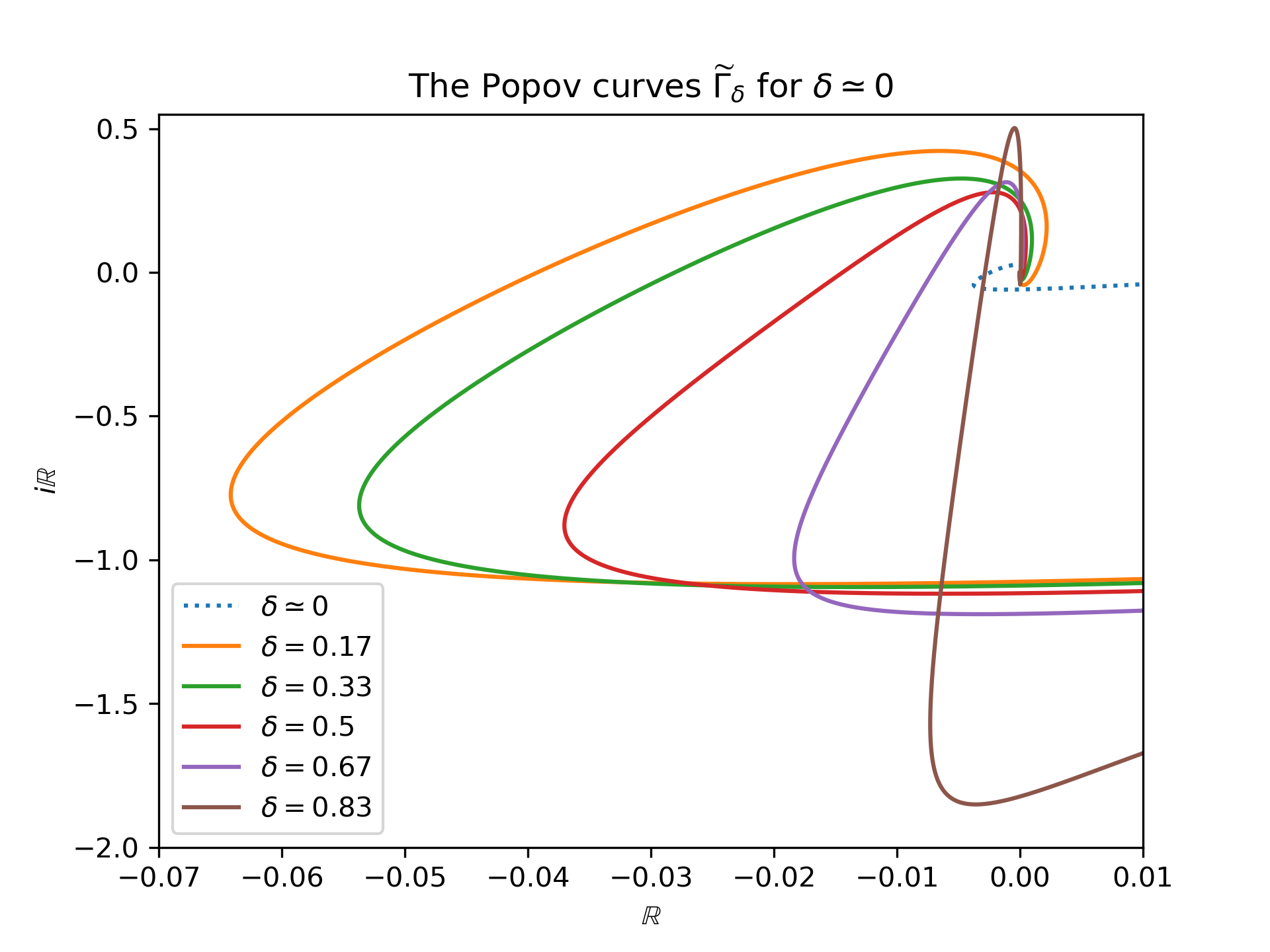
Figure 6. The Popov curves close to the limiting cases $\delta=0,1$.

The shape of the Popov curves found by the parameter study shown in Figure 6 suggests that to each $\delta\in(0,1)$ we can associate the uniquely determined line in $\mathbb{R}^{2}\cong\mathbb{C}$ that is tangent to $\Gamma_{\delta}(\omega)$ at its most negative intersection point with the real axis, i.e. where

$$\operatorname{Im}\Bigl{(}G_{\delta}\bigl{(}i\omega_{1}(\delta)\bigr{)}\Bigr{)}=0.$$

That line is obviously given by

$$F_{q(\delta),\beta(\delta)}(x,y):=y-\frac{1}{q(\delta)}x-\frac{1}{q(\delta)\,\beta(\delta)}=0,$$

where, using the coordinates

(5.22) $$\Gamma_{\delta}(\omega):=\bigl{(}x(\omega),y(\omega)\bigr{)}:=\Bigl{(}\operatorname{Re}\bigl{(}G_{\delta}(i\omega)\bigr{)},\>\omega\,\operatorname{Im}\bigl{(}G_{\delta}(i\omega)\bigr{)}\Bigr{)},$$

we set

$$\beta(\delta):=-\frac{1}{G_{\delta}(i\omega_{1}(\delta))}\text{ and }\frac{1}{q(\delta)}:=\frac{\dot{y}}{\dot{x}}\Big{|}_{\omega=\omega_{1}(\delta)}.$$

In spite of this numerical graphical evidence, which shows the existence of an optimal straight line satisfying the Popov criterion up to the maximal choice for the constant $\hat{\beta}_{1}(x_{0},L)=-1/G_{L,x_{0}}\bigl{(}i\,\omega_{1}(L,x_{0})\bigr{)}$, we chose to state Theorem 5.2 in a weaker form that does not rely on any numerical or graphical verification.

5.3. Numerical verification of the Popov criterion for $\beta\in\bigl{(}0,\beta(\delta)\bigr{]}$ in the case $L<\infty$

Before giving the proof of Theorem 5.2 we discuss how a numerical verification of the Popov criterion can be performed to see that $\bigl{(}0,\beta(\delta)\bigr{]}$ is the maximal interval of global stability for the trivial equilibrium of (1.2). Here we again rescale units of length so that for $\delta\in(0,1)$ we can consider the transfer function

$$G_{\delta}(i\omega)=\frac{\sinh(\delta\sqrt{i\omega})}{2\sqrt{i\omega}\cosh(\sqrt{i\omega})},\>\omega\geq 0.$$

While we proceed in the spirit of the proof of Proposition 5.14, we need to resort to numerical computations to check the sign of the resulting elementary function. In order to express the imaginary and the real part of $G_{\delta}(i\omega)$ explicitly in a concise manner we set

$$A_{1}:=A_{1}(\delta,\omega)=\cosh\bigl{(}\delta\sqrt{\omega/2}\bigr{)}\sin\bigl{(}\delta\sqrt{\omega/2}\bigr{)}\text{ and }A_{2}:=A_{2}(\delta,\omega)=\cos\bigl{(}\delta\sqrt{\omega/2}\bigr{)}\sinh\bigl{(}\delta\sqrt{\omega/2}\bigr{)}$$

as well as

(5.23) $$B_{1} :=B_{1}(\omega)=\cos\bigl{(}\sqrt{\omega/2}\bigr{)}\cosh\bigl{(}\sqrt{\omega/2}\bigr{)}+\sin\bigl{(}\sqrt{\omega/2}\bigr{)}\sinh\bigl{(}\sqrt{\omega/2}\bigr{)}$$

(5.24) $$B_{2} :=B_{2}(\omega)=\cos\bigl{(}\sqrt{\omega/2}\bigr{)}\cosh\bigl{(}\sqrt{\omega/2}\bigr{)}-\sin\bigl{(}\sqrt{\omega/2}\bigr{)}\sinh\bigl{(}\sqrt{\omega/2}\bigr{)}$$

and

$$D:=D(\omega)=\sqrt{2\omega}\Big{[}\cos(\sqrt{2\omega})+\cosh(\sqrt{2\omega})\Bigr{]}.$$

The one can write

$$\operatorname{Re}\bigl{[}G_{\delta}(i\omega)\bigr{]}=\frac{1}{D}\langle A,B\rangle,\>\operatorname{Im}\bigl{[}G_{\delta}(i\omega)\bigr{]}=\frac{1}{D}\det(A,B),$$

with

$$\langle A,B\rangle:=A_{1}B_{1}+A_{2}B_{2}\text{ and }\det(A,B):=A_{1}B_{2}-A_{2}B_{1}.$$

Using the coordinate representation (5.22) of the Popov curve, an explicit representation of

$$\frac{1}{q(\delta)}:=\frac{\dot{y}}{\dot{x}}\Big{|}_{\omega=\omega_{1}(\delta)}$$

can be found in the form

(5.25) $$\frac{1}{q(\delta)}=\omega_{1}(\delta)\Big{\{}\frac{\det(\dot{A},B)+\det(A,\dot{B})}{\langle\dot{A},B\rangle+\langle A,\dot{B}\rangle-\langle A,B\rangle\dot{D}/D}\Big{\}}\Big{|}_{\omega=\omega_{1}(\delta)}.$$

The dotted quantities are differentiated with respect to $\omega$ and evaluated at $\omega_{1}(\delta)$. This representation is not fully explicit since a numerical root finding procedure needs to be used in order to locate the first positive solution $\omega_{1}(\delta)$ of $\operatorname{Im}\bigl{[}G_{\delta}(i\omega)\bigr{]}=\frac{1}{D}\det(A,B)=0$. In principle, for any given $\delta\in(0,1)$, the zero $\omega_{1}(\delta)$ can be determined with arbitrary (finite) precision. Therefore, for each $\delta\in(0,1)$, the verification of the Popov criterion

(5.26) $$F_{q(\delta),\beta(\delta)}(\omega):=y(\omega)-\frac{1}{q(\delta)}x(\omega)-\frac{1}{q(\delta)\,\beta(\delta)}\leq 0\text{ for }\omega>0,$$

up to the numerical determination of $\omega_{1}(\delta)$, consists in verifying that the following combination of the elementary functions $A_{i},B_{i},D$ is nonpositive, i.e., that

(5.27) $$F_{q(\delta),\beta(\delta)}(\omega)=\omega\det(A,B)/D-\frac{1}{q(\delta)}\Bigl{[}\langle A,B\rangle/D-\big{\langle}A\bigl{(}\omega_{1}(\delta)\bigr{)},B\bigl{(}\omega_{1}(\delta)\bigr{)}\big{\rangle}/D\bigl{(}\omega_{1}(\delta)\bigr{)}\Bigr{]}\leq 0\text{ for }\omega>0,$$

where $\frac{1}{q(\delta)}$ is given by (5.25). It is clear by the definition of $F_{q(\delta),\beta(\delta)}$, as well as directly by inspection of the above formula, that $F_{q(\delta),\beta(\delta)}\bigl{(}\omega_{1}(\delta)\bigr{)}=0$ which reflects the tangency condition. The verification of condition (5.27) can thus be performed by evaluation of the above expression over a finite range for $\omega$. This follows from the fact that we know that the curve $\Gamma_{\delta}(\cdot)$ spirals into the origin of the complex plane exponentially fast. Clearly the statement of nonpositivity requires a parametric study for $\delta$ in $(0,1)$. It can be verified analytically that

$$\lim_{\delta\to 0}\omega_{1}(\delta)q(\delta)=1\text{ and }\lim_{\delta\to 1}\omega_{1}(\delta)q(\delta)=\frac{b_{\pi}}{d_{\pi}}=\frac{3\pi+4}{3\pi}.$$

Thus the limit $\delta\to 1$ corresponds to the case $L=\infty$, which is intuitively clear. In fact, observe that, owing to (5.18) and to (5.19), the product

$$\omega_{1}(x_{0})q(x_{0})=\frac{b_{\pi}}{d_{\pi}}=\frac{3\pi+4}{3\pi},$$

is an invariant of the one-parameter family of Popov curves $\big{\{}\Gamma_{x_{0}}\,\big{|}\,x_{0}>0\big{\}}$. By contrast, for $L<\infty$, the product $\omega_{1}(\delta)q(\delta)$ depends on $\delta$ but has the two known limits given above.
Based on the parameter study in Figure 7, we formulate the following conjecture. In order to safeguard rigour we are, somewhat reluctantly, forced to formulate the numerical result merely as a conjecture, since it must be conceded that any parameter study cannot replace a rigorous proof of the validity of (5.27) for arbitrary $\delta\in(0,1)$ in spite of the fact that the criterion could be checked up to arbitrary finite precision for any given specific $\delta\in(0,1)$.

Figure 7. Depicted is the function appearing in the Popov criterion (5.27) for various values of $\delta\in(0,1)$

Conjecture 5.16.

For any $\delta\in(0,1)$, let $\beta(\delta):=-1/G_{\delta}\bigl{(}i\omega_{1}(\delta)\bigr{)}$. Then, for any $\beta\in\bigl{(}0,\beta(\delta)\bigr{]}$, the pair $\beta$ and $q(\delta)>0$, given by (5.25), satisfies the Popov criterion, i.e. the inequality

(5.28) $$\operatorname{Re}\bigl{[}G_{\delta}(i\omega)\bigr{]}-q(\delta)\omega\operatorname{Im}\bigl{[}G_{\delta}(i\omega)\bigr{]}\geq-\frac{1}{\beta}$$

for all $\omega\in\mathbb{R}\setminus\{0\}$.

We finally prove the theorem as it was formulated at the beginning of this section, i.e. without making any reference to the conjecture above.

Proof of Theorem 5.2

The proof relies on the application of the criterion derived in Proposition 5.10. For arbitrary fixed $L>x_{0}>0$ we look for a parameter value $\widehat{\beta}_{1}(x_{0},L)>0$ such that, for any $\beta\in\bigl{(}0,\widehat{\beta}_{1}(x_{0},L)\bigr{)}$, it is possible to find $q(x_{0})>0$ such that

$$\widehat{a}_{L}(\omega)+q(x_{0})\,\widehat{a_{L}^{\prime}}(\omega)-\frac{1}{\beta}\leq 0\text{ for }\omega>0.$$

This then entails that all solutions of the Volterra integral equation (5.1) with arbitrary parameters $x_{0}>0$ and $L>x_{0}$ converge to zero as $t\to\infty\,$ as long as $\beta\in\bigl{(}0,\widehat{\beta}_{1}(x_{0},L)\bigr{)}$. If this is the case, we call $\bigl{(}0,\widehat{\beta}_{1}(x_{0},L)\bigr{)}$ an interval of stability for the integral equation with parameters $L>x_{0}>0$. We define the Popov curve associated with $x_{0}$ and $L$ by

$$\Gamma_{x_{0},L}(\omega)=\bigl{(}x(\omega),y(\omega)\bigr{)}=\Bigl{(}\operatorname{Re}\bigl{[}G_{x_{0},L}(i\omega)\bigr{]},\>\omega\,\operatorname{Im}\bigl{[}G_{x_{0},L}(i\omega)\bigr{]}\Bigr{)}.$$

By introducing the functional

$$F_{q,\beta}(x,y)=y-\frac{x}{q}-\frac{1}{q\,\beta}\,,$$

the verification of the stability criterion reduces to showing that suitable choices of the parameters $\beta$ and $q$ lead to

$$F_{q,\beta}\bigl{(}\Gamma_{x_{0},L}(\omega)\bigr{)}\leq 0,\>\omega>0.$$

For arbitrary $x_{0}>0$ and $L>x_{0}$ we set

(5.29) $$\widehat{\beta}_{1}(x_{0},L)=\frac{1}{M(x_{0},L)\,q(x_{0})}$$

where

$$q(x_{0})=\frac{x_{0}^{2}}{d_{\pi}},\,d_{\pi}=\frac{9\pi^{3}}{8\pi+\frac{32}{3}}$$

and

$$M(x_{0},L):=\max\limits_{\omega>0}\Bigl{\{}\omega\,\operatorname{Im}\bigl{[}G_{x_{0},L}(i\omega)\bigr{]}-\frac{1}{q(x_{0})}\operatorname{Re}\bigl{[}G_{x_{0},L}(i\omega)\bigr{]}\Bigr{\}}.$$

To show that the above maximum exists and that it is positive, observe that, by definition, the Popov set $\Omega^{\text{Pop}}_{L,x_{0}}$ contains a minimal element $\omega_{1}>0$ such that

$$\operatorname{Im}\bigl{[}G_{x_{0},L}(i\omega_{1})\bigr{]}=0\text{ and }\operatorname{Re}\bigl{[}G_{x_{0},L}(i\omega_{1})\bigr{]}<0.$$

This shows that $\widehat{\beta}_{1}(x_{0},L)>0$, if the maximum exists. In order to obtain the existence of the maximum a simple calculation yields that

$$H(\omega) :=\omega\,\operatorname{Im}\bigl{[}G_{x_{0},L}(i\omega)\bigr{]}-\frac{1}{q(x_{0})}\operatorname{Im}\bigl{[}G_{x_{0},L}(i\omega)\bigr{]}=$$

(5.30) $$\frac{\sqrt{\omega}}{2}\operatorname{Im}\Bigl{[}\;\overline{\sqrt{i}}\,\big{\{}\cosh(x_{0}\sqrt{i\omega})\tanh(L\sqrt{i\omega})-\sinh(x_{0}\sqrt{i\omega})\big{\}}\Bigr{]}$$

$$-\frac{d_{\pi}}{2\,x_{0}^{2}\,\sqrt{\omega}}\operatorname{Re}\Bigl{[}\;\overline{\sqrt{i}}\,\big{\{}\cosh(x_{0}\sqrt{i\omega})\tanh(L\sqrt{i\omega})-\sinh(x_{0}\sqrt{i\omega})\big{\}}\Bigr{]}.$$

Then notice that $\lim_{\omega\to 0^{+}}H(\omega)$ exists and that

$$\lim_{\omega\to 0^{+}}H(\omega)\;<0.$$

One also has that

$$\lim_{\omega\to\infty}H(\omega)=0,$$

which is verified by using

$$\lim_{\omega\to\infty}\tanh(L\sqrt{i\omega})=1,$$

and that

$$\lim_{\omega\to\infty}\sqrt{\omega}\Bigl{[}\cosh(x_{0}\sqrt{i\omega})\tanh(L\sqrt{i\omega})-\sinh(x_{0}\sqrt{i\omega})\Bigr{]}=0.$$

To study $\lim_{\omega\to 0^{+}}H(\omega)$, one observes that

$$\lim_{\omega\to 0^{+}}\frac{\overline{\sqrt{i}}}{\sqrt{\omega}}\Bigl{[}\cosh(x_{0}\sqrt{i\omega})\tanh(L\sqrt{i\omega})-\sinh(x_{0}\sqrt{i\omega})\Bigr{]}>0.$$

Since $H(\omega)$ is negative for sufficiently small arguments, converges to zero as $\omega\to\infty$, and has positive values, the maximum must be attained and be positive. Now for any $\beta\in\bigl{(}0,\widehat{\beta}_{1}(x_{0},L)\bigr{)}$, we obtain the estimate

$$F_{q(x_{0}),\beta}\bigl{(}\Gamma_{x_{0},L}(\omega)\bigr{)}<F_{q(x_{0}),\widehat{\beta}_{1}(x_{0},L)}\bigl{(}\Gamma_{x_{0},L}(\omega)\bigr{)},\>\omega>0.$$

It only remains to verify that

$$F_{q(x_{0}),{\widehat{\beta}}_{1}(x_{0},L)}\bigl{(}\Gamma_{x_{0},L}(\omega)\bigr{)}=H(\omega)-\frac{1}{q(x_{0})\,\widehat{\beta}_{1}(x_{0},L)}\leq 0,\>\omega>0,$$

which follows from the definition of $\widehat{\beta_{1}}(x_{0},L)$ since

$$F_{q(x_{0}),\widehat{\beta}_{1}(x_{0},L)}\bigl{(}\Gamma_{x_{0},L}(\omega)\bigr{)}\leq\max\limits_{\omega>0}H(\omega)-\frac{1}{q(x_{0})\widehat{\beta}_{1}(x_{0},L)}=M(x_{0},L)-\frac{1}{q(x_{0})\,\widehat{\beta}_{1}(x_{0},L)}=0.$$

Next we present the argument producing the alternative interval of stability $\bigl{(}0,\beta_{1}(x_{0})\bigr{)}=(0,\frac{c_{\pi}}{x_{0}})$ for any $x_{0}>0$ and all sufficiently large $L>x_{0}$. For fixed $x_{0}>0$, we have shown in Remark 5.11 that

$$G_{x_{0},L}(i\omega)\to G_{x_{0}}(i\omega)\text{ as }L\to\infty,$$

uniformly for $\omega$ in intervals of the form $(c,\infty)$ with arbitrary $c>0$. This also implies that

$$\Gamma_{x_{0},L}(\omega)\to\Gamma_{x_{0}}(\omega)\text{ in }\mathbb{C}\text{ as }L\to\infty,$$

and that

$$F_{q(x_{0}),\beta_{1}(x_{0})}\bigl{(}\Gamma_{x_{0},L}(\omega)\bigr{)}\to F_{q(x_{0}),\beta_{1}(x_{0})}\bigl{(}\Gamma_{x_{0}}(\omega)\bigr{)}\text{ as }L\to\infty,$$

uniformly for $\omega$ in $(c,\infty)$ with arbitrary $c>0$. Hence, for any $\varepsilon>0$ and any $c>0$, there exists $C(\varepsilon,c)>0$ such that

$$F_{q(x_{0}),\beta_{1}(x_{0})}\bigl{(}\Gamma_{x_{0},L}(\omega)\bigr{)}\leq F_{q(x_{0}),\beta_{1}(x_{0})}\bigl{(}\Gamma_{x_{0}}(\omega)\bigr{)}+\varepsilon\text{ for }L\geq C(\varepsilon,c),$$

and $\omega\in(c,\infty)$. For any $\beta\in\bigl{(}0,\beta_{1}(x_{0})\bigr{)}$ we can choose $\delta(\beta):=\frac{\delta}{q(x_{0})}\bigl{[}\frac{1}{\beta}-\frac{1}{\beta_{1}(x_{0})}\bigr{]}$, $\delta\in(0,1)$, to obtain

$$F_{q(x_{0}),\beta}\bigl{(}\Gamma_{x_{0},L}(\omega)\bigr{)}+\delta(\beta)\leq F_{q(x_{0}),\beta_{1}(x_{0})}\bigl{(}\Gamma_{x_{0},L}(\omega)\bigr{)}\text{ for }\omega>0.$$

Thus, for $L\geq C\bigl{(}\delta(\beta),c\bigr{)}$ and for $\omega\in(c,\infty)$ we have that

$$F_{q(x_{0}),\beta}\bigl{(}\Gamma_{x_{0},L}(\omega)\bigr{)}+\delta(\beta)\leq F_{q(x_{0}),\beta_{1}(x_{0})}\bigl{(}\Gamma_{x_{0},L}(\omega)\bigr{)}\leq F_{q(x_{0}),\beta_{1}(x_{0})}\bigl{(}\Gamma_{x_{0}}(\omega)\bigr{)}+\delta(\beta).$$

Consequently, by Proposition 5.14, it holds that

$$F_{q(x_{0}),\beta}\bigl{(}\Gamma_{x_{0},L}(\omega)\bigr{)}\leq F_{q(x_{0}),\beta_{1}(x_{0})}\bigl{(}\Gamma_{x_{0}}(\omega)\bigr{)}\leq 0$$

for $L\geq C\bigl{(}\delta(\beta),c\bigr{)}$ and $\omega\in(c,\infty)$. Since we know from the first part of the proof that

$$\lim_{\omega\to 0^{+}}F_{q(x_{0}),\beta}\bigl{(}\Gamma_{x_{0},L}(\omega)\bigr{)}<-\frac{1}{\beta q(x_{0})}<0,$$

and $c>0$ can be chosen arbitrarily small, the inequality

$$F_{q(x_{0}),\beta}\bigl{(}\Gamma_{x_{0},L}(\omega)\bigr{)}\leq 0,$$

holds for $\omega\in(0,\infty)$ and $L\geq C(x_{0})$ for a large enough $C(x_{0})>0$. ∎

6. Global stability and Hopf bifurcation results for the nonlinear PDE

The stability result obtained in the previous section for the Volterra integral equation will now be applied to the nonlinear partial differential equation (1.2). It will be instrumental to infer the decay of the solutions of the PDE from the decay of the associated solutions of the integral equation. The following proposition is proved in [16, Proposition 2.3.] in a slightly different setting, yet its proof can readily be adapted to the present situation.

Proposition 6.1.

For fixed parameters $\beta,L\in(0,\infty)$ and $x_{0}\in(0,L)$ consider orbits $\Phi_{\beta}(\cdot,u_{0})$ of the semiflow $\bigl{(}\Phi_{\beta},\operatorname{H}_{L}^{1}\bigr{)}$ associated with (1.2). Then, as $t\to\infty\,$, for any $u_{0}\in\operatorname{H}_{L}^{1}$, it holds that

$$\Phi_{\beta}(t,u_{0})\longrightarrow 0\text{ in }\operatorname{H}_{L}^{1}\iff\bigl{(}\Phi_{\beta}(t,u_{0})\bigr{)}(x_{0})\longrightarrow 0\text{ in }\mathbb{R}.$$

Proof.

“$\Rightarrow$”: If $\Phi_{\beta}(t,u_{0})\to 0$ as $t\to\infty$, then the operation of “taking the trace” defines a bounded linear operator $\gamma_{x_{0}}\in\mathcal{L}(\operatorname{H}_{L}^{1},\mathbb{R})$ and therefore its continuity implies

$$\gamma_{x_{0}}\bigl{(}\Phi_{\beta}(t,u_{0})\bigr{)}=\bigl{(}\Phi_{\beta}(t,u_{0})\bigr{)}(x_{0})\to 0\text{ as }t\to\infty.$$

“$\Leftarrow$”: If $y(t):=\bigl{(}\Phi_{\beta}(t,u_{0})\bigr{)}(x_{0})\to 0$ as $t\to\infty$, then by (5.1) we have that

$$\lim_{t\to\infty}y(t)=\lim_{t\to\infty}\Bigl{[}g_{L}(t)+\int_{0}^{t}a_{L}(t-\tau)f\bigl{(}\beta u(\tau,x_{0})\bigr{)}\,d\tau\Bigr{]}\,=\,0,$$

which entails

$$\lim_{t\to\infty}\int_{0}^{t}a(t-\tau)f\bigl{(}\beta u(\tau,x_{0})\bigr{)}\,d\tau=0,$$

since we know by the properties of the semigroup $e^{-tA_{L}}$ that $\lim_{t\to\infty}g_{L}(t)=0$. Next notice that, for arbitrary $x\in(-L,L)$, it holds that

$$u(t,x):=\Phi_{\beta}(t,u_{0})(x)=\bigl{(}e^{-tA_{L}}u_{0}\bigr{)}(x)+\int_{0}^{t}k_{L}(t-\tau,x)f\bigl{(}\beta u(\tau,x_{0})\bigr{)}\,d\tau,$$

where, by definition (5.4), it holds that

$$k_{L}(t,x)=-a_{L}(t,x)=-\bigl{(}e^{-tA_{L}}\delta_{0}\bigr{)}(x).$$

Again from $\lim_{t\to\infty}\bigl{(}e^{-tA_{L}}u_{0}\bigr{)}(x)=0$ we obtain

(6.1) $$\lim_{t\to\infty}u(t,x)=-\lim_{t\to\infty}\int_{0}^{t}k_{L}(t-\tau,x)f\bigl{(}\beta u(\tau,x_{0})\bigr{)}\,d\tau,\>x\neq x_{0}.$$

Since we know by assumption that $\lim_{t\to\infty}f\bigl{(}\beta u(\tau,x_{0})\bigr{)}=0$ and, by inserting the spectral decomposition (3.2) of $k_{L}$ in (6.1), we conclude similarly as in [16] that for arbitrary $x\in(-L,L)$ and $t\to\infty$

$$\lim_{t\to\infty}u(t,x)=0\;,$$

i.e. we obtain the pointwise convergence of $\Phi_{\beta}(t,u_{0})$ to the zero function.
To prove that convergence to zero also occurs in the topology of $\operatorname{H}_{L}^{1}$ we use (4.1) to derive the equation satisfied by $\hat{u}_{n}(t)$, which is the $n$-th coefficient in the spectral basis expansion of the solution

$$u(t,x)=\sum_{k=1}^{\infty}\langle u(t,\cdot),\varphi_{k}\rangle\varphi_{k}(x)=\sum_{k=1}^{\infty}\hat{u}_{k}(t)\varphi_{k}(x).$$

Observe that the $\operatorname{H}^{1}$ norm of a function $u(t,\cdot)$ of $x$ obtained for fixed $t$ is equivalent to

$$\|u(t,\cdot)\|_{\operatorname{H}_{L}^{1}}^{2}=\sum_{k=1}^{\infty}(1+k^{2})|\hat{u}_{k}|^{2}.$$

This is seen by extending $u(t,\cdot)$ to a periodic function ${\tilde{u}}(t,\cdot)$ by reflection as described in (3.3) and noticing the direct relation between the standard Fourier series of $\tilde{u}$ and the spectral basis expansion of $u\,$. We also use the fact that $u\in\operatorname{H}_{L}^{1}$ if and only if $\tilde{u}\in\operatorname{H}^{1}_{\pi}(-2L,2L)$, where the index indicates periodicity.
Next look at the evolution of the single modes of the solution, which is determined by

$$\hat{u}_{n}(t)=e^{-t\lambda_{L,n}^{2}}\,\langle\hat{u}_{0},\varphi_{L,n}\rangle-\int_{0}^{t}f\bigl{(}\beta u(\tau,x_{0})\bigr{)}e^{-(t-\tau)\lambda_{L,n}^{2}}\,d\tau.$$

A simple calculation exploiting the boundedness of $f$ then yields

$$(1+n^{2})\big{|}\hat{u}_{n}(t)\big{|}^{2}\leq c(1+n^{2})|\hat{u}_{0n}|+\frac{c}{\lambda_{L,n}^{4}}(1+n^{2}),\>n\geq 1.$$

This, together with the fact that $u_{0}\in\operatorname{H}^{1}$ and that $\lambda_{L,n}^{4}\sim n^{4}$ as $n\to\infty$, implies that the series

(6.2) $$\sum_{n\geq 1}(1+n^{2})|\hat{u}_{n}(t)|^{2}$$

converges uniformly in $t\geq 0$. This shows that the tail of the Fourier representation of the solution can be made smaller than any given $\varepsilon>0$ independently of $t\geq 0$. For the remaining finitely many terms, a direct estimate of the integral yields smallness. It namely follows from the solution representation that

$$|\hat{u}_{n}(t)| \leq e^{-t\lambda_{L,0}t}|\widehat{u_{0}}_{n}|+\int_{0}^{t_{\varepsilon}}e^{-(t-\tau)\lambda_{L,0}^{2}}\,d\tau+\max_{\tau\geq t_{\varepsilon}}|f\bigl{(}\beta u(\tau,x_{0})|\int_{t_{\varepsilon}}^{t}e^{-(t-\tau)\lambda_{L,0}^{2}}\,d\tau$$

$$\leq e^{-(t-t_{\varepsilon})\lambda_{L,0}^{2}}\Big{\{}|\widehat{u_{0}}_{n}|+\frac{1}{\lambda_{L,0}^{2}}\Big{\}}+c\max_{\tau\geq t_{\varepsilon}}|f\bigl{(}\beta u(\tau,x_{0})|\leq\varepsilon$$

for $t$ large enough. This shows that

$$\sum_{n\geq 1}(1+n^{2})|\hat{u}_{n}(t)|^{2}\to 0\text{ as }t\to\infty,$$

or, in other words that $u(t)\to 0$ in $\operatorname{H}^{1}$. ∎

We can now proceed to summarize the main results of our analysis.

Theorem 6.2.

For arbitrary choice of the paramters $L>x_{0}>0$ the following assertions hold:

• There exsist $\varepsilon>0$ such that for any $\beta\in\bigl{(}\beta_{1}(x_{0},L),\beta_{1}(x_{0},L)+\varepsilon\bigr{)}$, with

  $$\beta_{1}(x_{0},L)=-\frac{1}{G_{L,x_{0}}\bigl{(}i\omega_{1}(L,x_{0})\bigr{)}}\text{ and }\omega_{1}(L,x_{0})=\min\Omega^{Pop}_{L,x_{0}},$$

  the semiflow $\bigl{(}\Phi_{\beta},\operatorname{H}_{L}^{1}\bigr{)}$ associated with (1.2)${}_{L,x_{0}}$ possesses a non-trivial periodic orbit.

• For $\beta\in\bigl{(}0,\widehat{\beta_{1}}(x_{0},L)\bigr{)}$ where $\widehat{\beta}_{1}(x_{0},L)>0$ is defined in (5.29), every (semi-)orbit of the semiflow $\bigl{(}\Phi_{\beta},\operatorname{H}_{L}^{1}\bigr{)}$ associated with (1.2)${}_{L,x_{0}}$ converges to zero as $t\to\infty$.

• If we assume that $L\geq C(x_{0})$ for some sufficiently large constant $C(x_{0})$, then for any $\beta\in\bigl{(}0,\beta_{1}(x_{0})\bigr{)}=\bigl{(}0,\frac{c_{\pi}}{x_{0}}\bigr{)}$, for $c_{\pi}=\frac{3\pi}{\sqrt{2}}e^{\frac{3\pi}{4}}$, every (semi-)orbit of the semiflow $\bigl{(}\Phi_{\beta},\operatorname{H}_{L}^{1}\bigr{)}$ associated with (1.2)${}_{L,x_{0}}$ converges to zero as $t\to\infty$.

Proof.

The second and third assertion follows directly from our main result on the Volterra integral equation, Theorem 6.1, and from Proposition 5.2.
The first statement is a consequence of the general results obtained in [2, Theorem 1],[22, Theorem I.8.2.], or [27]. They can be applied analogously as in [14]. We have shown in Proposition 2.5 and in our discussion of the Popov set that

$$\sigma\bigl{(}A_{\beta_{1}(x_{0},L)}\bigr{)}\cap i\mathbb{R}=\big{\{}\pm i\omega_{1}(L,x_{0})\big{\}}.$$

The non-degeneracy condition for the crossing of the imaginary axis by the complex conjugate pair of eigenvalues of the operator $-A_{\beta}$ needs to be checked to conclude the proof. We need to verify that

$$\frac{d}{d\beta}\operatorname{Re}\bigl{[}\lambda(\beta)\bigr{]}\,\Big{|}_{\beta=\beta_{1}(x_{0},L)}>0,$$

where, for some $\varepsilon>0$, there exists

$$\lambda:\Bigl{(}\beta_{1}(x_{0},L)-\varepsilon,\beta_{1}(x_{0},L)+\varepsilon\Bigr{)}\to\mathbb{C}\text{ with }\lambda\bigl{(}\beta_{1}(x_{0},L)\bigr{)}=+i\omega_{1}(L,x_{0}),$$

i.e. a local parametrization of the eigenvalue’s path as it crosses the imaginary axis in the complex upper halfplane as $\beta$ increases. This follows from Proposition 3.5 and Remark 3.7. ∎

Remark 6.3.

Supported by numerical evidence, we conjecture that the definition (5.29) leads to

$$\widehat{\beta_{1}}(x_{0},L)=\beta_{1}(x_{0},L)=-\frac{1}{G_{L,x_{0}}\bigl{(}i\,\omega_{1}(L,x_{0})\bigr{)}}\text{ with }\omega_{1}(L,x_{0})=\min\Omega^{Pop}_{L,x_{0}}.$$

We note that one inequality $\widehat{\beta_{1}}(x_{0},L)\leq\beta_{1}(x_{0},L)$ follows from the knowledge that the asymptotic stability of the equilbrium $u=0$ is lost at $\beta_{1}(x_{0},L)$ due to the Hopf bifurcation. Thus proving this conjecture reduces to showing $\widehat{\beta_{1}}(x_{0},L)\geq\beta_{1}(x_{0},L)$. This, in turn, would follow if we could verify that the value of $M(x_{0},L)$ in the definition (5.29) is achieved by $\omega_{1}(L,x_{0})$ as a maximizer. Clearly, if one were able to prove this statement then Conjecture 5.16 would no longer be needed. In that case the parameter range of global stability $(0,\widehat{\beta_{1}}(x_{0},L)\bigr{)}$ would be maximal due to $\widehat{\beta_{1}}(x_{0},L)=\beta_{1}(x_{0},L)$, i.e. the interval of stability constructed for the Volterra integral equation then extends up to the critical parameter value where the Hopf bifurcation occurs.

To discuss the stability of the bifurcating periodic solutions for the one-parameter family of semiflows $\bigl{(}\Phi_{\beta},\operatorname{H}_{L}^{1}\bigr{)},\>\beta>0$, observe that the Ljapunov-Schmidt reduction used in [1] to discuss the Hopf bifurcation phenomenon in the finite dimensional case leads to more precise statements about the structure of the bifurcating periodic solutions. In particular, the local uniqueness of the bifurcating solutions can be described in more detail and is made explicit in the next remark. As highlighted in [1] the Liapunov-Schmidt reduction, which the author applies to ODEs, can often be extended naturally to semi-flows in infinite dimensional phase spaces stemming from reaction-diffusions problems. We refrain from executing that approach here and refer to [2]. Instead we prefer to apply the results on the existence of a center manifold in the infinite dimensional situation. In fact, our problem, for $L<\infty$, formulated in the Sobolev space $\operatorname{H}_{L}^{1}$ falls into the rather general class of quasilinear parabolic systems discussed in [27]. The possibility to restrict our semiflow to its finite dimensional center manifold, allows us to discuss the stability of the bifurcating solutions by studying the ODE that governs the dynamics on the center manifold.

Remark 6.4.

For the stability analysis of the bifurcating periodic solutions the results in [1, Theorems 26.21 and 27.11] provide a more precise description of the local structure at the bifurcation locus. There exists $\varepsilon>0$ and a map

$$\Big{[}s\mapsto(u(s),T(s),\beta(s))\Big{]}\in C^{\infty}\Big{(}(-\varepsilon,\varepsilon)\;,\;\delta\mathbb{B}_{H^{1}_{L}}(0)\times\delta\mathbb{B}_{\mathbb{R}}(\frac{2\pi}{\omega_{1}(x_{0},L)})\times\delta\mathbb{B}_{\mathbb{R}}(\beta_{1}(x_{0},L))\Big{)}$$

with

$$\bigl{(}u(0),T(0),\beta(0)\bigr{)}=\bigl{(}0,\frac{2\pi}{\omega_{1}(x_{0},L)},\beta_{1}(x_{0},L)\bigr{)}\in H^{1}_{L}\times(0,\infty)\times(0,\infty),$$

for some suitably chosen factor $\delta>0$, that shrinks the open unit balls appropriately. The above map has the property that, for $0<s<\varepsilon$, the orbit of $u(s)$ under $\Phi_{\beta(s)}$ denoted by

$$\gamma(s):=\Big{\{}\Phi_{\beta(s)}(t,u(s))\,\big{|}\,t\geq 0\Big{\}}$$

is a noncritical periodic orbit of the semiflow $\bigl{(}\Phi_{\beta(s)},\operatorname{H}_{L}^{1}\bigr{)}$ with period $T(s)$ passing through the point $u(s)\in\delta\mathbb{B}_{H^{1}_{L}}(0)$ and with

(6.3) $$\gamma(s_{1})\neq\gamma(s_{2}),$$

for $0<s_{1}<s_{2}<\varepsilon$. Every noncritical periodic orbit of the semiflow $\bigl{(}\Phi_{\beta(s)},\operatorname{H}_{L}^{1}\bigr{)}$ in a sufficiently small neighbourhood of $\bigl{(}0,\frac{2\pi}{\omega_{1}(x_{0},L)},\beta_{1}(x_{0},L)\bigr{)}$ in the cartesian product $H^{1}_{L}\times(0,\infty)\times(0,\infty)$ is contained in the family

$$\big{\{}\gamma(s)\,\big{|}\,0<s<\varepsilon\big{\}}.$$

The map

$$\big{[}s\mapsto\beta(s)\big{]}\,:\,(0,\varepsilon)\rightarrow(0,\infty)$$

is injective. This follows directly from (6.3), since otherwise identical noncritical periodic orbits for $s_{1}\neq s_{2}$ could be obtained from $\beta(s_{1})=\beta(s_{2})$ and the identity of the semiflows $\bigl{(}\Phi_{\beta(s_{i})},\operatorname{H}_{L}^{1}\bigr{)}$, $i=1,2$.

Theorem 6.5.

Fix arbitrary $L>x_{0}>0$ and assume that, for any $\beta\in\bigl{(}0,\beta_{1}(x_{0},L)\bigr{)}$, the trivial solution of the semiflow $\bigl{(}\Phi_{\beta},\operatorname{H}_{L}^{1}\bigr{)}$ is globally asymptotically stable. Then the noncritical periodic orbits of the semiflow $\bigl{(}\Phi_{\beta},\operatorname{H}_{L}^{1}\bigr{)}$ originating from the Hopf bifurcation at $\beta_{1}(x_{0},L)>0$ are (orbitally) stable for any $\beta\in\bigl{(}\beta_{1}(x_{0},L),\beta_{1}(x_{0},L)+\delta\bigr{)}$ for some $\delta>0$. In fact, using the map $\big{[}s\mapsto\beta(s)\big{]}$ discussed in Remark 6.4, it holds that

$$\dot{\beta}(s)>0,$$

for $0<s<\varepsilon(\delta)$, which means that the Hopf bifuration at $\beta_{1}(x_{0},L)$ is supercritical.

Proof.

The map $\big{[}s\mapsto\beta(s)\big{]}:(0,\varepsilon)\rightarrow(0,\infty)$ is continuous and injective for $0<s<\varepsilon$. Hence it is strictly monotone on $(0,\varepsilon)$. Since $\beta(\cdot)$ is differentiable either $\dot{\beta}(s)<0$ or $\dot{\beta}(s)>0$ must hold for $s\in(0,\varepsilon)$. The case $\dot{\beta}(s)<0$ can be excluded since it implies the existence of a noncritical periodic orbit of the semiflow $\bigl{(}\Phi_{\beta},\operatorname{H}_{L}^{1}\bigr{)}$ for $\beta<\beta_{1}(x_{0},L)$. Since this cannot happen by Theorem 6.2 and by the assumption that $\bigl{(}0,\beta_{1}(x_{0},L)\bigr{)}$ is an interval of global stability for the trivial equilibrium, we conclude that $\dot{\beta}(s)>0$ and that the bifurcating noncritical periodic orbits are stable. ∎

Remark 6.6.

The assumption that the trivial solution of the semiflow $\bigl{(}\Phi_{\beta},\operatorname{H}_{L}^{1}\bigr{)}$ is globally asymptotically stable for any $\beta\in\bigl{(}0,\beta_{1}(x_{0},L)\bigr{)}$ can be dropped if either Conjecture 5.16 were shown to be true or if the condition $\widehat{\beta_{1}}(x_{0},L)=\beta_{1}(x_{0},L)$ discussed in Remark 6.3 were shown to hold.

The next result settles a conjecture formulated in [14, Remarks 4.4. (c)] for the problem (1.1). It was not stated in [16] even though, in the light of the above results, it is an immediate corollary to [16, Theorem 5.1.]. We add the result here for the sake of completeness and due to the fact that the conjecture in [14] provided the initial motivation for both [16] and the present paper.

Theorem 6.7.

The noncritical periodic orbits of the semiflow $\bigl{(}\Phi_{\beta},\operatorname{H}^{1}(0,\pi)\bigr{)}$ associated with (1.1) that originate from the Hopf bifurcation at $\beta_{0}\approx 5.6655$ are (orbitally) stable for $\beta\in(\beta_{0},\beta_{0}+\delta)$ for some $\delta>0$. In other words, the Hopf bifuration from the trivial solution at $\beta=\beta_{0}$ is supercritical.

Proof.

The statement follows analogously as in the proof of Theorem 6.5 since the trivial critical point of the semiflow $\bigl{(}\Phi_{\beta},\operatorname{H}^{1}(0,\pi)\bigr{)}$ is shown to be globally attractive on the maximal interval of stability, i.e. for $\beta\in(0,\beta_{0})$ in [16, Theorem 5.1.]. ∎

7. Implementation used in the numerical calculations

In order to generate Figures 1, 2, and 4, we made used of a discretization of the operator $A^{L}_{\beta}$ which is described in this section. As for Figures 3 and 5, the computations are based on the zeros of the spectrum determining functions $z_{L}$ found in (3.11) inside the proof of Proposition 3.5, and on (3.9), respectively. Since $A_{L,\beta}=A_{L}+\beta\delta_{0}\delta_{x_{0}}^{\top}$ and $A_{L}=A_{L,0}$ has an explicit spectral resolution in terms of its eigenvalues $\mu^{k}_{L,0}=\frac{\pi^{2}k^{2}}{4L^{2}}$, $k\in\mathbb{N}$, and eigenfunctions $\varphi_{k,L}=\frac{1}{\sqrt{L}}\sin\bigl{(}k\pi\,\frac{x+L}{2L}\bigr{)}$, we opt for a spectral discretization. In order to obtain it, we introduce the grid of equidistant points $x^{m}=(x^{m}_{k})_{k=1,\dots 2^{m}-1}$ given by

$$x^{m}_{k}=-L+k\frac{2L}{2^{m}},\>k=1,\dots,2^{m}-1,$$

and the discrete sine transform matrix $S_{m}$ with entries

$$S_{m}(k,j)=\varphi_{k,L}(x^{m}_{j}).$$

Then we approximate $A_{L}$ spectrally by

$$A_{L}^{m}=\frac{2L}{2^{m}}\,S_{m}^{\top}\operatorname{diag}\bigl{[}\frac{k^{2}\pi^{2}}{4L^{2}}\bigr{]}_{k=1,\dots,2^{m}-1}\,S_{m},$$

where $S_{m}^{\top}=S_{m}^{-1}$ and the scalar factor amounts to the application of the quadrature rule (the trapezoidal rule in this case) required in the discrete transform to approximate the corresponding continuous integral. The Dirac distribution supported at $y\in(-L,L)$ is also discretized spectrally as

$$\delta^{m}_{y}=\sum_{k=1}^{2^{m}-1}\varphi_{k,L}(y)\varphi_{k,L}(x^{m}).$$

This yields a spectral approximation through

$$\langle\delta_{y},u\rangle_{\operatorname{H}^{-1}_{L},\operatorname{H}^{1}_{L}}\simeq\frac{2L}{2^{m}}\bigl{(}\delta^{m}_{y}\bigr{)}^{\top}u^{m},$$

if $u^{m}$ is the vector approximating $u\in\operatorname{H}^{1}_{L}$. Again the scalar factor is dictated by the quadrature rule used to approximate the duality pairing. Finally the operator $A_{L,m}$ of interest is approximated by

$$A^{m}_{L,\beta}=A^{m}_{L}+\beta\frac{2L}{2^{m}}\delta^{m}_{0}\bigl{(}\delta^{m}_{x_{0}}\bigr{)}^{\top},$$

and its adjoint by the transpose $\bigl{(}A^{m}_{L,\beta}\bigr{)}^{\top}$. Again, this discretization is used for the spectral calculations leading to Figures 1, 2, and 4.

References

- [1] H. Amann. Ordinary Differential Equations. de Gruyter, Berlin, 1990.
- [2] H. Amann. Hopf bifurcation in quasilinear reaction-diffusion systems. In Delay Differential Equations and Dynamical Systems, volume 1455 of Lect. Notes in Math. Springer Verlag, Berlin, 1991.
- [3] H. Amann. Linear and Quasilinear Parabolic Problems. Birkhäuser, Basel, 1995.
- [4] W. Arendt, C.J.K. Batty, M. Hieber, and F. Neubrander. Vector-valued Laplace transforms and Cauchy problems, volume 96 of Monographs in Mathematics. Birkhäuser Verlag, Basel, 2001.
- [5] W. Arendt and A. Rhandi. Perturbations of positive semigroups. Arch. Math., 56:107–119, 1991.
- [6] R. Curtain and K. Morris. Transfer functions of distributed parameter systems: A tutorial. Automatica, 45(5):1101–1116, 2009.
- [7] D. Daners and J. Glück. A Criterion for the Uniform Eventual Positivity of Operator Semigroups. Integral Equations and Operator Theory, 90(4):19 pp., 2018.
- [8] D. Daners, J. Glück, and J.B. Kennedy. Eventually and asymptotically positive semigroups on Banach lattices. J. Differential Equations, 261(5):2607–2649, 2016.
- [9] D.S. de Cássia, R. Broche, L.A.F. de Oliveira, and A.L. Pereira. Global attractor for an equation modelling a thermostat. Electron. J. Differential Equations, 2003(100):7 pp, 2003.
- [10] W. Desch and W. Schappacher. Some Perturbations Results for Analytic Semigroups. Mathematische Annalen, 281:157–162, 1988.
- [11] G. B. Folland. Real analysis: modern techniques and their applications. Wiley, New York, 1984.
- [12] J. A. Goldstein. Semigroups of Linear Operators and Applications. Oxford University Press, Oxford, 1985.
- [13] M. Gonzalez, M. Gualdani, and J. Solà Morales. Instability and Bifurcation in a Trend Depending Pricing Model. Acta Aplicandae Mathematicae, 144(1):121–136, 2013.
- [14] P. Guidotti and S. Merino. Hopf bifurcation in a scalar reaction diffusion equation. Journal of Differential Equations, 140(1):209–222, 1997.
- [15] P. Guidotti and S. Merino. Gradual loss of positivity and hidden invariant cones in a scalar heat equation. Differential and Integral Equations, 13(10–12):1551–1568, 2000.
- [16] P. Guidotti and S. Merino. On the Maximal Parameter Range of Global Stability for a Nonlocal Thermostat Model. Submitted, arXiv:1909.08589, 2020.
- [17] G. Infante and J. R. L. Webb. Loss of positivity in a nonlinear scalar heat equation. NoDEA Nonlinear Differential Equations Appl., 13:249–261, 2006.
- [18] G. Infante and J. R. L. Webb. Nonlinear nonlocal boundary value problems and perturbed Hammerstein integral equations. Proc. Edinb. Math. Soc., 49:637–656, 2006.
- [19] G. Kalna and S. McKee. The thermostat problem with a nonlocal nonlinear boudary condition. IMA J. Appl. Math., 69(5):437–462, 2004.
- [20] T. Kato. Perturbation Theory for Linear Operators. Springer Verlag, New York, 1966.
- [21] T. Kato. Perturbation Theory for Linear Operators. Classics in Mathematics. Springer Verlag, Berlin, Heidelberg New York, 1980.
- [22] H. Kielhöfer. Bifurcation Theory, volume 156 of Applied Mathematical Sciences. Springer, New York, 2012.
- [23] S.D. Lawley. Blowup from Randomly Switching between Stable Boundary Conditions for the Heat Equation. Commun. Math. Sci., 16(4):1131–1154, 2018.
- [24] Peter Linz. Analytical and numerical methods for Volterra equations. Number 7 in SIAM studies in applied mathematics. SIAM, Philadelphia, 1985.
- [25] R.K. Miller. Nonlinear Volterra Integral Equations. Mathematics Lecture Notes Series. W.A. Benjamin, Menlo Park, CA, 1971.
- [26] A. Pazy. Semigroups of Linear Operators and Application to Partial Differential Equations. Springer Verlag, New York, 1983.
- [27] G. Simonett. Center manifolds for quasilinear reaction-diffusion systems. Differential and Integral Equations, 8(4):753–796, 1995.
- [28] Kôsaku Yosida. Functional Analysis, volume 123 of Die Grundlehren der matematischen Wissenschaft. Springer Verlag, Berlin, Heidelberg, New York, 1974.