Graph Neural Network Based Coarse-Grained Mapping Prediction

Abstract

The selection of coarse-grained (CG) mapping operators is a critical step for CG molecular dynamics (MD) simulation. It is still an open question about what is optimal for this choice and there is a need for theory. The current state-of-the art method is mapping operators manually selected by experts. In this work, we demonstrate an automated approach by viewing this problem as supervised learning where we seek to reproduce the mapping operators produced by experts. We present a graph neural network based CG mapping predictor called Deep Supervised Graph Partitioning Model(DSGPM) that treats mapping operators as a graph segmentation problem. DSGPM is trained on a novel dataset, Human-annotated Mappings (HAM), consisting of 1,206 molecules with expert annotated mapping operators. HAM can be used to facilitate further research in this area. Our model uses a novel metric learning objective to produce high-quality atomic features that are used in spectral clustering. The results show that the DSGPM outperforms state-of-the-art methods in the field of graph segmentation. Finally, we find that predicted CG mapping operators indeed result in good CG MD models when used in simulation.

1 Introduction

Coarse grained (CG) models can be viewed as a two part problem of selecting a suitable CG mapping and a CG force field. In this work we focus on addressing the issue of CG mapping selection for a given system. A CG mapping is a representation of how atoms in a molecule are grouped to create CG beads. Once the CG mapping is selected, CG force field parameters required for the CG simulation can be determined via existing bottom-up¹⁷ or top-down³¹ CG methods. The former use atomistic simulations for parameterization of the CG force fields while the latter use experimental data.

Conventionally, a CG mapping for a molecule is selected using chemical and physical intuition. For example, the widely used MARTINI CG model uses mapping of four heavy (non-hydrogen) atoms to one CG bead as chosen by experts²⁵. Another popular choice of CG mapping for proteins and peptides is to assign one CG bead centered at the $\alpha$-carbon for each amino acid. These choices are not built on any thermodynamic or theoretical argument. A recent discussion on commonly used mapping strategies is summarized in Ingólfsson et al. ¹⁶. There have been recent efforts in developing systematic and automated methods in selecting a CG mapping for a molecule. Automation of CG mapping is important to enhance scalability and transferability.

Webb et al. ³⁶ proposed a spectral and progressive clustering on molecular graphs to identify vertex groups for subsequent iterative bond contractions that lead to CG mappings with hierarchical resolution. Wang and Gómez-Bombarelli ³⁵ developed an auto-encoder based method that simultaneously learns the optimal CG mapping of a given resolution and the corresponding CG potentials. mappingEnt proposed a mapping entropy based method to simplify the model representation of biomolecules. Their thoeretical model focuses on preserving most information content in the lower resolution model compared to the all atom model. Chakraborty et al. ⁴ reported a hierarchical graph method where multiple mappings of a given molecule are encoded in a hierarchical graph, which can further be used to auto-select a particular mapping using algorithms like uniform-entropy flattening⁴⁰. In a recent systematic study on the effects of CG resolution on reproducing on and off target properties of a system, Khot et al. ²¹ hypothesized that low-resolution CG models might be information limited, instead of having a representability limitation. This hypothesis suggests that there might be ways of enhancing the information of CG models without increasing their dimension and complexity. This is supported by a recent study of 26 CG mappings for 7 alkane molecules that found little correlation between mapping resolution and CG model performance ^{Chakraborty2020b}. There is not only a lack of methods to compute mapping operators, there is no agreed upon goal in choosing mapping operators.

Mapping operators used in practice for CG simulations are usually rule-based ^{25, 16},but recent advances have been made in algorithmic ^{4, 36, 41, 1, 12, 24} and unsupervised methods¹³. Rule-based schemes have fixed resolution and must be created for each molecular functional group, limiting their application to sequence-defined biomolecules or polymers. Algorithmic and unsupervised methods have only been qualitatively evaluated on specific systems. The Chakraborty et al. ⁴, Gómez-Bombarelli et al. ¹³ methods also required explicit molecular dynamics simulations, which leads to questions about hyperparameters (e.g., sampling, atomistic force field) and requires at least hours per system. Such methods also are not learning nor optimizing mapping operator correctness directly. Supervised learning has not been used in previous work because there are no datasets and no obvious optimality criteria.

Here we have avoided the open question of "which is the best mapping?", by choosing to match human intuition, the main selection method of past mapping operators. We demonstrate a supervised learning based approach using a graph neural network framework, Deep Supervised Graph Partitioning Model(DSGPM). To train and evaluate the DSGPM, we compiled a Human-annotated Mappings (HAM) dataset with expert annotated CG mappings of 1,206 organic molecules, where each molecule has one or more coarse graining annotations by human experts. We expect this dataset can facilitate research on coarse graining and the graph partition problem. The HAM database allows DSGPM to learn CG mappings directly from annotations. Our framework is closely related to the problem of graph partitioning and has molecular feature extraction and embedding as major components. The graph neural network is trained via metric learning objectives to produce good atom embeddings of molecular graph, which creates better affinity matrix for spectral clustering ²⁷. Should there be a consensus in the field on what are “best” mappings, our model can be easily adapted to match a new dataset of annotations.

2 Related Work

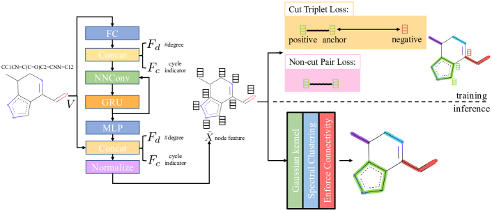
Figure 1: Overview of the method. Adjacency matrix $E$ is omitted from the figure. FC stands for fully-connected layer and MLP stands for multilayer perceptron. Concat denotes concatenation. NNConv and GRU are explained in Eq. 1 and Eq. 2, respectively. “Normalize” means $L_{2}$ normalization.

2.1 Molecular Feature Extraction

The applications of graph convolutional neural networks (GCNN) to molecular modeling is an emerging approach for “featurizing” molecular structures. Featurizing a molecule is a challenging process which extracts useful information from a molecule to a fixed representation. This is important since conventional machine learning algorithms can accept only a fixed length input. However, a molecule can have arbitrary sizes and varying connectivities. GCNNs have become a useful tool for molecular featurization as they can be used for deep learning of raw representations of data which are less application specific unlike molecular fingerprints. Kearnes et al. ²⁰ have shown in their work that GCNNs can be used to extract molecular features with little preprocessing as possible. Furthermore, it is shown that the results from the GCNN are comparable to neural networks trained on molecular fingerprint representations. Wu et al. ³⁹ have implemented a GCNN featurization method in MoleculeNet. The GCNN is used to compute an initial feature vector which describe an atom’s chemical environment and a neighbor list for each atom³⁹. Additionally, they show that unlike the fingerprints methods, GCNNs create a learnable process to extract molecular features using differentiable network layers. Gilmer et al. ¹¹ have developed a generalized message passing nerural network (MPNN) to predict molecular properties. In this work, authors have used a GCNN to extract molecular features and to learn them from molecular graphs. The authors also state that there is a lack of a generalized framework which can work on molecular graphs for feature extraction. Given the proven success of GCNNs in feature extraction, the motivation for our work was to develop a generalized deep learning based method apt for chemistry problems.

2.2 Graph Partitioning and Graph Neural Network

If a molecule is viewed as a graph, the problem of selecting a CG mapping is analogous to partitioning the molecular graph. While there has been limited application of molecular graph for the purpose of selecting CG mappings, as discussed earlier, we would like to highlight some strategies employed for problems relevant to graph partitioning. Spectral clustering ^{37, 18, 27} is one of the baseline method used in graph clustering task. Compared with Expectation-Maximization (EM) ⁷, spectral clustering has a better modeling on pairwise affinity given by the adjacency matrix of a graph. METIS ¹⁹ solves the graph partition problem in a multilevel scheme via coarsening, partition, and refinement steps. Graclus ⁸ proposed a generalized kernel k-means method with better speed, memory efficiency, and graph clustering result. Fortunato ¹⁰ has a comprehensive review of the methods developed for community detection in graphs. Safro et al. ³² compared different graph coarsening schemes for graph partitioning using algebraic distance between nodes of the graph. Recently, some graph neural network ² based graph partitioning methods have been proposed. GAP ²⁶ uses graph neural networks to predict node-partition assignment probability, which is learned through normalized cut loss and balanced cut loss. ClusterNet ³⁸ adds differentiable k-means clustering at the end of graph neural network to enable end-to-end training. Compared to the aforementioned methods, our DSGPM combines the advantages of both spectral clustering and a graph neural network, leading to better results than either alone. We also propose and justify a novel metric learning loss to train the graph neural network.

2.3 Metric Learning

The goal of the metric learning is to learn a model which encodes the input data to an embedding space, where embeddings (usually represented by fixed length vector) of similar data objects are separated by short distances in the embedding space and different data objects are separated by larger distances in the embedding space. Hadsell et al. ¹⁴ proposed a siamese network trained via contrastive loss which 1) minimizes $L_{2}$ distance for instances from the same group, and 2) maximizes $L_{2}$ distance for instances from the different groups if the $L_{2}$ distance is larger than a margin. Instead of only considering a pair of data, Schroff et al. ³³ considered a triplet of data $\langle$anchor, positive, negative$\rangle$ and triplet loss to ensure $L(\text{anchor},\text{negative})$ (distance between anchor and negative) should be larger than $L(\text{anchor},\text{positive})$ (distance between anchor and positive) by a margin. However, the methods above have only been applied to nonstructural data (e.g., image clustering). Furthermore, one of challenging problem is sampling pairs or triplets of data from the dataset. In contrast, our proposed method can efficiently enumerate pairs or triplets by explicitly treating the graph structure.

3 Method

3.1 Problem Formulation

Deep Supervised Graph Partitioning Model (DSGPM)  formulates the CG mapping prediction as a graph partitioning problem. Suppose $Q$ is the set of atom types existing in the dataset. An atom in a molecule is represented as a one-hot encoding of its atom type. Similarly, a bond is represented as a one-hot encoding of its bond type (e.g., single, double, aromatic, etc.). Therefore, a molecule with $n$ atoms is formulated as a graph $G=(V,E)$ , where $V\in\mathbb{R}^{n\times|Q|}$ represents atoms and $E\in\mathbb{R}^{n\times n\times 4}$ denotes the adjacency matrix with encoded bond types.

3.2 Motivation

One strong baseline method to solve the graph partitioning problem is spectral clustering ²⁷. The performance of spectral clustering is mainly decided by the quality of affinity matrix $S\in\mathbb{R}^{n\times n}$, where $S_{ij}$ denotes the affinity (ranging from 0 to 1) between vertex $i$ and vertex $j$. In this task, the adjacency matrix (ignoring bond type information in $E$) can serve as the affinity matrix fed into spectral clustering. However, for the CG mapping prediction problem, an ideal affinity matrix should have low affinity value of cut (edge connecting two atoms from different CG beads) and high affinity of an edge which is not a cut, while adjacency matrix only contains “0”s and “1”s to represent the existence of edges.

3.3 Deep Supervised Graph Partitioning Model

The main difference from the baseline method is a graph neural network $\mathcal{F}$ that is used to obtain a better affinity matrix, where $\mathcal{F}$ follows the architecture design of MPNN ¹¹. The overview of the method is shown in Fig. 1. With the molecular graph $G$ as the input, $\mathcal{F}$ extracts $q$-dimensional atom features $\tilde{X}\in\mathbb{R}^{n\times q}$ through message passing (i.e., $\tilde{X}=\mathcal{F}(G)$). Concretely, $\mathcal{F}$ first uses a fully-connected layer to project one-hot atom type encoding into the feature space. Then, we concatenate the embedded feature with two numbers: 1) number of degree; 2) cycle indicator (i.e., whether the atom is in a cycle) (zero or one) to obtain $d$-dimensional feature $X^{0}\in\mathbb{R}^{n\times d}$. We find out that adding these two features improves the result (Sec. 4.5). Next, $X^{0}$ is iteratively updated $T$ time steps to obtain $X^{T}$:

$$\hat{X}^{t-1}_{u} =\mathbf{W}^{\prime}X^{t-1}_{u}+\sum_{v\in\mathcal{N}(u)}X^{t-1}_{v}\phi^{e}(E_{uv}),$$ (1)

$$X^{t}_{u} =\text{GRU}(\hat{X}^{t-1}_{u},H^{t-1}_{u}),$$ (2)

where underscript $u$ denotes $u$-th atom and superscript $t$ denotes time step; $\mathcal{N(\cdot)}$ denotes the set of neighboring nodes of the given vertex; $\mathbf{W}\in\mathbb{R}^{d\times d}$ is a weight matrix; superscript ^′ denotes transpose; $\phi^{e}(\cdot):\{0,1\}^{4}\mapsto\mathbb{R}^{d\times d}$ is function mapping bond type to edge-conditioned weight matrix, which is implemented as multilayer perceptron; GRU stands for Gated Recurrent Unit ⁶. Finally, the output feature $\tilde{X}$ is obtained by:

$$\tilde{X}^{\prime} =\text{Concat}(\text{MLP}(X^{T}),V,F_{d},F_{c}),$$ (3)

$$\tilde{X} =\frac{\tilde{X}^{\prime}}{||\tilde{X}^{\prime}||_{2}},$$ (4)

where Concat denotes concatenation; MLP denotes multilayer perceptron; $F_{d}\in\mathbb{N}^{n}$ denotes degree of each atom and $F_{c}\in\{0,1\}^{n}$ is cycle indicator (i.e.whether an atom is in a cycle).

After computing the atom feature $\tilde{X}$, the affinity matrix $A\in\mathbb{R}^{n\times n}$ can be calculated by a Gaussian kernel:

$$A_{ij}=\exp\left(\frac{-||\tilde{X}_{i}-\tilde{X}_{j}||_{2}^{2}}{2\sigma^{2}}\right)\tilde{E},$$ (5)

where $\sigma$ is the bandwidth and is set to $\sigma=1$ in the experiment. $\tilde{E}\in\mathbb{R}^{n\times n}$ denotes the adjacency matrix ($\tilde{E}_{ij}=1$ if atom $i$ and atom $j$ are bonded, otherwise $\tilde{E}_{ij}=0$).

Therefore, in order to obtain a good affinity matrix, $||\tilde{X}_{i}-\tilde{X}_{j}||_{2}$ should be large when edge $\langle i,j\rangle$ is a cut and small when edge $\langle i,j\rangle$ is not a cut. Hence, by utilizing the ground-truth partition $B\in\mathbb{N}^{n}$ ($B_{i}$ denotes coarse grain (partition) index of $i$-th atom), we design Cut Triplet Loss and Non-cut Pair Loss to guide the network outputting good node feature $\tilde{X}$ during training.

3.4 Training

3.4.1 Cut Triplet Loss.

The goal of Cut Triplet Loss is to push pairs of node embeddings far away from each other when they belong to different partitions. To this end, we first extract all triplets from the given molecular graph $G$ where each triplet contains three atoms: (anchor atom, positive atom, negative atom) denoted by $\{\mathtt{a,p,n}\}$ such that $B_{\mathtt{a}}=B_{\mathtt{p}}$ but $B_{\mathtt{a}}\neq B_{\mathtt{n}}$ (see “green” features and “red” feature on top-right of Fig. 1). In other words, we extract non-cut edge $\langle\mathtt{a},\mathtt{p}\rangle$ and cut edge $\langle\mathtt{a},\mathtt{n}\rangle$ sharing one common vertex $\mathtt{a}$. The set of triplets is denoted by $P$. Then, Cut Triplet Loss is defined by:

$$L_{\text{triplet}}=\frac{1}{|P|}\sum_{\begin{subarray}{c}P_{i}=\{\mathtt{a,p,n}\}\\ i\in[1,|P|]\end{subarray}}\text{max}(||\tilde{X}_{\mathtt{a}}-\tilde{X}_{\mathtt{p}}||_{2}-||\tilde{X}_{\mathtt{a}}-\tilde{X}_{\mathtt{n}}||_{2}+\alpha,0),$$ (6)

where $\alpha$ is a hyperparameter denoting the margin in triplet loss. By optimizing Cut Triplet Loss, the objective $||\tilde{X}_{\mathtt{a}}-\tilde{X}_{\mathtt{p}}||_{2}+\alpha\leq||\tilde{X}_{\mathtt{a}}-\tilde{X}_{\mathtt{n}}||_{2}$ can be satisfied for all triplets.

3.4.2 Non-cut Pair Loss.

The purpose of Non-cut Pair Loss is to pull pairs of node embeddings as close as possible when they are from the same partition. Therefore, all pairs of node $\mathtt{a}$ and $\mathtt{a}^{\prime}$ are extracted when edge $\langle\mathtt{a},\mathtt{a}^{\prime}\rangle$ is not a cut. The set of pairs of node is denoted as $S$. Then, Non-cut Pair Loss is defined by:

$$L_{\text{pair}}=\frac{1}{|S|}||\tilde{X}_{\mathtt{a}}-\tilde{X}_{\mathtt{a}^{\prime}}||_{2}.$$ (7)

The final loss function to train the network is defined by:

$$L=L_{\text{triplet}}+\lambda L_{\text{pair}},$$ (8)

where the coefficient is taken to be $\lambda=0.1$.

3.5 Inference

In the inference stage, we first apply Eq. 5 on the extracted node feature $\tilde{X}$. Then, based on affinity matrix $A$, spectral clustering is used to obtain the graph clustering result. Note that graph clustering is slightly different to graph partitioning. The latter requires the predicted partition must be a connected-component. Hence, we post-process the graph clustering result by enforcing connectivity of each graph partition: for each predicted graph cluster, if it contains more than one connected-component, we assign new indices to each connected-components.

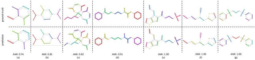
Figure 2: Visualization of the CG mapping prediction and the ground-truth. Atoms and corresponding edges belongs to the same CG bead are highlighted with the same color. Cut edges are not highlighted (i.e., in black). Note that colors between prediction and ground-truth may not match since colors are randomly selected.

4 Experiment

4.1 Dataset

Human-annotated Mappings (HAM) dataset  contains CG mappings of 1,206 organic molecules with less than 25 heavy atoms. Each molecule was downloaded from the PubChem database as SMILES ²². One molecule was assigned to two annotators to compare the human agreement between CG mappings. These molecules were hand-mapped using a web-app. The completed annotations were reviewed by a third person, to identify and remove unreasonable mappings which did not agree with the given guidelines. Hence, there are 1.68 annotations per molecule in the current database (16% removed). To preserve the chemical and physical information of the all atom structure accurately, the annotators were instructed to group chemically similar atoms together into CG beads while preserving the connectivity of the molecular structure. They were also instructed to preserve the planar configuration of rings if possible by grouping rings into 3 or more beads.

4.2 Evaluation Metrics

Adjusted Mutual Information (AMI) ³⁴ is used to evaluate the graph partition result in terms of nodes in the graph. Nodes from the same CG bead are assigned with the same cluster index and AMI compares predicted nodes’ cluster indices with ground-truth nodes’ cluster indices. We also evaluate graph partition result in terms of accuracy of predicting cuts from a graph. We report the precision, recall, and F1-score on cuts prediction (denoted by Cut Prec., Cut Recall, and Cut F1-score, respectively). Our method is trained and evaluated through 5-fold cross-validation ²³ to mitigate the bias of data split. Concretely, the dataset is split into 5 non-overlapping partitions (i.e., one molecule only exists in one data partition). The experiment will run 5 iterations. At $i$-th iteration ($i\in[1,5]$), the $i$-th split of the dataset is regarded as testing set (ground-truth partition $B$ is not used) and rest 4 splits of the dataset is regarded as the training set (ground-truth partition $B$ is used for training). Therefore, after training, DSGPM is evaluated on unseen molecules in the testing set. The final results are the average values over all iterations. Since one molecule may have multiple annotations, we choose one of the annotations that produces the best result for both AMI and cut accuracy.

4.3 Implementation Details

DSGPM is trained with at most 500 epochs and we choose the epoch at which model achieves the best performance over the 5-fold cross validation . The hidden feature dimension is 128. The implementation of spectral clustering used in the inference stage is from Scikit-learn ³⁰. Since spectral clustering requires a hyperparameter to indicate the expected number of clusterings, we provide the ground-truth number of clusters based on CG annotations. Cycles of each molecular graph are obtained via “cycle_basis” ²⁹ function implemented by NetworkX ¹⁵. The code of graph neural network is based on PyTorch ²⁸ and PyTorch Geometric ⁹.

Method	AMI	Cut Prec.	Cut recall	Cut F1-score
GAP 26	0.33	0.47	0.73	0.54
Graclus 8	0.45	0.58	0.81	0.65
ClusterNet 38	0.52	0.64	0.62	0.58
METIS 19	0.56	0.63	0.56	0.58
Cut Cls.	0.67	0.75	0.73	0.73
Spec. Cluster. 27	0.73	0.75	0.75	0.75
DSGPM (Ours)	0.79	0.80	0.80	0.80
Human	0.81	0.81	0.81	0.81

Table 1: Comparison with state-of-the-art methods. Average results over 5-fold cross validation are shown. Here, “Spec. Cluster.” means spectral clustering. The standard deviation of 5-fold cross-validation result under all evaluation metrics of our method is smaller than 0.01. Evaluation on human agreement (last row) is based on 128 molecules with 129 pairs of mappings, where mappings in each have the same number of CG beads.

4.4 Comparison with State-of-the-Art

We compare our method with five state-of-the-art graph partitioning methods. We used officially released code of the comparing methods on HAM dataset. Here, we also show an alternative of our method (denoted by Cut Cls.): by regarding the graph partitioning problem of edge cut binary classification problem (i.e., predicting the probability that an edge is a cut or not), we train DSGPM with binary cross-entropy loss. In the inference stage, we rank “cut probability” of each edge in descending order and take top-$k$ edges as the final cut prediction, where $k$ is the ground-truth number of cuts computed from the CG annotation. The result of comparison is shown in Tab. 1. The result shows that our method outperforms all state-of-the-art methods in terms of both AMI and cut accuracy. Moreover, DSGPM also outperforms Cut Cls., proving the effectiveness the metric learning training objectives and the importance of spectral clustering stage in our method. Additionally, by treating one annotation as prediction and the other annotation as ground-truth, we can show the agreement between different annotations (see last row in Tab. 1), which can be regarded as human annotator’s performance. The result shows that our proposed DSGPM is very closed to human-level performance.

input	AMI	Cut Prec.	Cut Recall	Cut F1-score
w/o $F_{d}$ & $F_{c}$	0.781	0.797	0.801	0.798
w/o $F_{c}$	0.783	0.800	0.803	0.801
w/o $F_{d}$	0.790	0.806	0.807	0.806
DSGPM	0.790	0.806	0.809	0.807

Table 2: Ablation study on the input of DSGPM. $F_{d}$ and $F_{c}$ denote number of degree and cycle indicator, respectively.

loss terms	AMI	Cut Prec.	Cut Recall	Cut F1-score
w/o $L_{\text{triplet}}$	0.73	0.75	0.76	0.7
w/o $L_{\text{pair}}$	0.78	0.80	0.80	0.80
DSGPM	0.79	0.80	0.80	0.80

Table 3: Ablation study on loss terms. $L_{\text{triplet}}$ denotes Cut Triplet Loss and $L_{\text{pair}}$ denotes Non-cut Pair Loss.

$\lambda$	AMI	Cut Prec.	Cut Recall	Cut F1-score
0.1	0.79	0.80	0.80	0.80
0.5	0.78	0.80	0.80	0.80
1	0.78	0.80	0.80	0.80
2	0.78	0.80	0.80	0.80
10	0.78	0.80	0.80	0.80

Table 4: Ablation study on loss terms. $\lambda$ denotes the coefficient for Non-cut Pair Loss (Eq. 8).

$\sigma$	AMI	Cut Prec.	Cut Recall	Cut F1-score
0.5	0.77	0.79	0.79	0.79
1	0.79	0.80	0.80	0.80
1.5	0.77	0.79	0.79	0.79
2	0.76	0.78	0.78	0.78

Table 5: Ablation study on bandwidth of Gaussian kernel. $\sigma$ denotes the bandwidth for Gaussian kernel in Eq. 5.

4.5 Ablation Study

We study the contribution of degree and cycle indicator in the input. The results are shown in Tab. 2. Degree feature (w/o $F_{c}$ in Tab. 2) improves the edge-based metrics (cut precision, cut recall, cut F1-score) and cycle indicator (w/o $F_{d}$ in Tab. 2) contributes to all evaluation metrics. Combining both input feature boosts the performance further.

We also examined the contribution of each loss terms, cut triplet loss and non-cut pair loss. The result in Tab. 3 shows that Cut Triplet Loss plays the major role in the training objective and combining both loss terms will produce better performance, which proves that $L_{\text{triplet}}$ and $L_{\text{pair}}$ ’s objectives, separating atoms connected by an cut edge and concentrating features of atoms from the same partition, are reciprocal during training.

Furthermore, we study the impact of different values for the hyperparameters $\lambda$ (see Eq. 8) and $\sigma$ (see Eq. 5) in Tab. 4 and Tab. 5, respectively. The ablation results show that DSGPM is not sensitive to changes of $\lambda$ and choosing $\sigma=1$ yields best results.

4.6 Visualization

4.6.1 CG Mapping Result

We visualize the CG mapping prediction results against ground-truth in Fig. 2. Predicted mappings (e)-(g) are indistinguishable from the human annotations. Even though AMI values of structures (a)-(c) are comparatively lower, our predictions in (a)-(c) are still able to capture the essential features such as functional groups and ring conformations from the ground truth mappings. (a),(b),(e)-(g) also show that when rings in molecules are grouped into three CG beads by the human annotators, DSGPM model is able to capture this pattern. When rings are grouped into one CG bead (2 (d)), the model similarly chose this. Overall this shows that DSGPM can reproduce mappings which are significantly close to the human annotations. We have further compared our predictions with the widely used MARTINI mapping scheme. Results are shown in Fig. S3 in the SI.

4.6.2 SARS-CoV-2 Structure Prediction

Using our trained DSGPM, we predict the CG mappings for previously unseen SARS-CoV-2 protease structure (PDB ID:6M03³). In Fig. 3 we compare our result with three baseline methods. Even though our training dataset did not contain peptide sequences we show that our model is capable of predicting CG mappings of complex proteins. We see in Fig. 3 that our prediction is similar to predicted mapping from the spectral clustering method. This is an expected result as we use spectral clustering in the inference stage of our model. In spectral clustering, METIS methods and our model the resolution of the CG mapping can be controlled as the number of partitions is a hyper parameter. Mappings predicted by these three methods in Fig.3 contain 32 beads. However, in the Graclus method the resolution cannot be controlled. In Fig. 3 d), the predicted mapping from Graclus method contain 1455 CG beads. This is not a reasonable prediction as the fine grain structure contains 2367 atoms.

To gain a better understanding of the mappings, in Fig. S1 in the SI, we use the FASTA representation of the SARS-CoV-2 protease and color each one-letter code by the color of the CG beach to which each alpha-carbon belong. We see that our model is able to group amino acids with reasonable cuts along the backbone of the protein. Our model and spectral clustering method group 7-11 amino acids while the METIS method group 2-11 amino acids into CG beads. This shows that while DSGPM is capable of predicting state-of-the-art mapping for small molecules it can also be scaled to predict reasonable mappings for arbitrarily large structures.

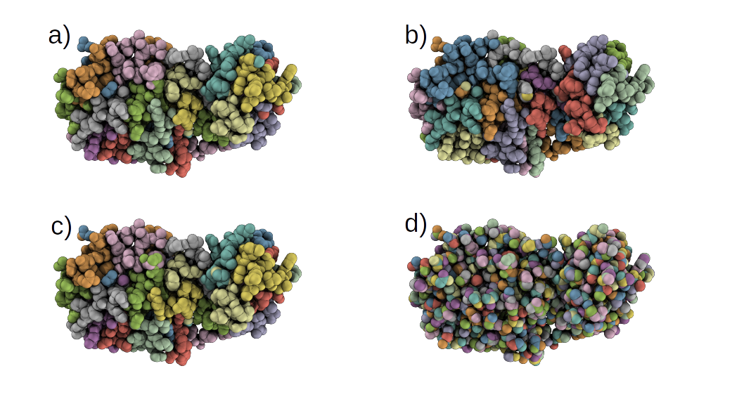
Figure 3: Comparison of CG mappings of SARS-CoV-2 protease structure predicted by baseline methods, a) our DSGPM model b) METIS¹⁹ c) Spectral clustering²⁷ d) Graclus⁸ . a), b) and c) have 32 CG beads while d) contains 1455 CG beads.

4.6.3 Model Performance in CG Simulations

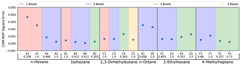
Figure 4: COM-RDF square errors as previously reported for CG mappings of 6 alkane molecules ^{Chakraborty2020b}. The mappings for each molecule have been categorized into colored blocks corresponding to the number of CG beads. For each block, the mappings are arranged in the order of increasing AMI values, as indicated below the CG mapping labels.

Thus far, the model has been judged against Human-annotated Mappings and not in molecular dynamics simulation. To assess the predicted mappings, we draw upon the simulation results from recent work by Chakraborty2020b where force matching was used for coarse-graining. We have compared the performance of the CG mappings predicted by DSGPM for 6 alkane molecules with multiple CG bead numbers, giving 22 different simulation results. The individual mappings of the 6 alkane molecules (n-hexane, isohexane, 2,3-dimethylbutane, n-octane, 3-ethylhexane, and 4-methylheptane) that were considered in Chakraborty2020b and those predicted by DSGPM are shown in Fig. S2. DSGPM predicts one mapping per molecule/bead number. To assess the quality of these mappings, we show how the CG simulation error changes for mappings other than the predicted DSGPM mapping as measured by AMI. Decreasing error as a AMI increases (better performance as we get closer to the DSGPM prediction) indicates good model performance. Fig. 4 shows the square errors for center-of-mass (COM) radial distribution function (RDF) relative to the all atom simulation as previously reported ^{Chakraborty2020b} for each of the 6 alkane molecules. For a given molecule, the mappings are categorized into colored blocks corresponding to the number of beads in the CG mapping. AMI values of the mappings are computed relative to the CG mappings from DSGPM with the same number of CG beads. The mappings within the same colored block are arranged in increasing order of AMI values. It is observed that for most of the alkanes, a mapping with higher AMI compared to another with equal number of beads, yields lower COM-RDF square error (6 instances). 4 bead 3-ethylhexane mappings and 3 bead 4-methylheptane mappings are the only instances where a mapping with higher AMI gives higher COM-RDF square error than a comparable mapping with lower AMI. Thus the mappings predicted by DSGPM have good performance when used in simulations as judged from this small dataset of 22 simulations.

5 Conclusion

In this work, we propose a novel DSGPM as a supervised learning method for predicting CG mappings. By selecting good inputs and designing novel metric learning objectives on graph, the graph neural network can produce good atom features, resulting in better affinity matrix for spectral clustering. We also report the first large-scale CG dataset with experts’ annotations. The result shows that our method outperforms state-of-the-art methods by a predicting mappings which are nearly indistinguishable from human annotations. The ablation study found that the novel loss term is the key innovation of the model. Furthermore, we show that our automated model can be used to predict CG mappings for macromolecules even though the training set was of small molecules and the CG mappings do result in good performance when implemented in force-matched CG simulations.

6 Conflicts of interest

There are no conflicts to declare.

7 Acknowledgements

This material is based upon work supported by the National Science Foundation under Grant No. 1764415. We thank the Center for Integrated Research Computing at the University of Rochester for providing the computational resources required to complete this study. Part of this research was performed while the authors were visiting the Institute for Pure and Applied Mathematics (IPAM), which is supported by the National Science Foundation (Grant No. DMS-1440415).

8 Supplementary Information

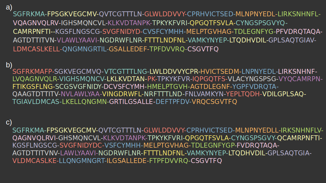
Figure 5: Comparison of FASTA representations of the SARS-CoV-2 main protease coarse grained mappings predicted by DSGPM model with baseline methods. Predicted mappings from a) our DSGPM model b) METIS¹⁹ and c) Spectral clustering²⁷ are illustrated. All three mappings presented here have 32 CG beads. We have colored each one-letter label of amino acids by the color of CG bead to which each alpha-carbon belong.

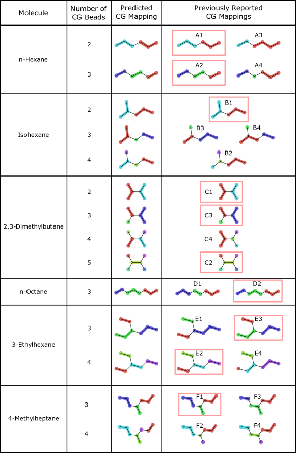
Figure 6: Illustrations of previously studied CG mappings of 6 alkane molecules ^{Chakraborty2020b} (n-hexane, isohexane, 2,3-dimethylbutane, n-octane, 3-ethylhexane, and 4-methylheptane) and DSGPM predicted CG mappings of the 6 molecules with varying CG bead number. The mappings enclosed in red boxes correspond highlight instances where the predicted mappings are identical to one of previously studied mappings with the same number of CG beads and hence have AMI value as 1.

Peptide Sequence Mapping

We have considered 4 penta-peptides to compare the predicted CG mappings from DSGPM to the corresponding MARTINI CG models. The amino-acid sequence for the 4 peptides is of the form GGXGG, where G is glycine and X is either alanine (A), valine (V), aspartic acid (D) or tyrosine (Y). Note that peptides are previously unseen by the DSGPM model. For each of the peptides, we set the partition number hyperparameter for DSGPM to be equal to the number of CG beads in its MARTINI CG model. The MARTINI CG models for G and A have one bead each, those for V and D have two beads each and the CG model for Y has 4 beads. Hence, the number of partition hyperparameter for DSGPM was set as 5 for GGAGG, 6 for GGVGG and GGDGG, and 8 for GGYGG. Fig. 7 shows the predicted CG mappings along with the MARTINI CG models for the 4 penta-peptides. The predicted CG mappings closely mirror the MARTINI models for GGAGG, GGVGG and GGDGG, albeit with some deviations. The most prominent difference between the predicted result and the MARTINI CG model is observed for GGYGG.

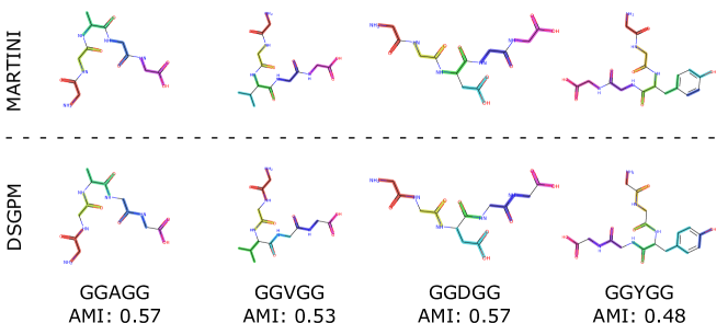
Figure 7: Visualization of CG mappings for 4 peptides. We compare the CG mappings predicted by DSGPM to the corresponding mappings determined by the widely used MARTINI method. Atoms and their adjacent bonds belonging to the same CG bead are highlighted with the same color.

References

- Arkhipov et al. 2006 Anton Arkhipov, Peter L Freddolino, and Klaus Schulten. Stability and Dynamics of Virus Capsids Described by Coarse-Grained Modeling. Structure, 14(12):1767–1777, dec 2006. ISSN 09692126. doi: 10.1016/j.str.2006.10.003.
- Battaglia et al. 2018 Peter W Battaglia, Jessica B Hamrick, Victor Bapst, Alvaro Sanchez-Gonzalez, Vinicius Zambaldi, Mateusz Malinowski, Andrea Tacchetti, David Raposo, Adam Santoro, Ryan Faulkner, et al. Relational inductive biases, deep learning, and graph networks. arXiv preprint arXiv:1806.01261, 2018.
- Berman et al. 2000 Helen M. Berman, John Westbrook, Zukang Feng, Gary Gilliland, T. N. Bhat, Helge Weissig, Ilya N. Shindyalov, and Philip E. Bourne. The protein data bank. Nucleic Acids Res, 28:235–242, 2000.
- Chakraborty et al. 2018 Maghesree Chakraborty, Chenliang Xu, and Andrew D White. Encoding and selecting coarse-grain mapping operators with hierarchical graphs. The Journal of Chemical Physics, 149(13):134106, 2018.
- Chakraborty et al. 2019 Maghesree Chakraborty, Jinyu Xu, and Andrew White. Is preservation of symmetry necessary for coarse-graining? chemrxiv preprint chemrxiv.10728128.v1, Nov 2019. doi: 10.26434/chemrxiv.10728128.v1.
- Cho et al. 2014 Kyunghyun Cho, Bart van Merriënboer, Dzmitry Bahdanau, and Yoshua Bengio. On the properties of neural machine translation: Encoder–decoder approaches. In Proceedings of SSST-8, Eighth Workshop on Syntax, Semantics and Structure in Statistical Translation, pages 103–111, Doha, Qatar, October 2014. Association for Computational Linguistics. doi: 10.3115/v1/W14-4012. URL https://www.aclweb.org/anthology/W14-4012.
- Dempster et al. 1977 Arthur P Dempster, Nan M Laird, and Donald B Rubin. Maximum likelihood from incomplete data via the em algorithm. Journal of the Royal Statistical Society: Series B (Methodological), 39(1):1–22, 1977.
- Dhillon et al. 2007 I. S. Dhillon, Y. Guan, and B. Kulis. Weighted graph cuts without eigenvectors a multilevel approach. IEEE Transactions on Pattern Analysis and Machine Intelligence, 29(11):1944–1957, Nov 2007. ISSN 1939-3539. doi: 10.1109/TPAMI.2007.1115.
- Fey and Lenssen 2019 Matthias Fey and Jan Eric Lenssen. Fast graph representation learning with pytorch geometric. In International Conference on Learning Representations Workshop, 2019.
- Fortunato 2010 Santo Fortunato. Community detection in graphs. Phys. Rep., 486(3-5):75–174, 2010. ISSN 03701573. doi: 10.1016/j.physrep.2009.11.002. URL http://dx.doi.org/10.1016/j.physrep.2009.11.002.
- Gilmer et al. 2017 Justin Gilmer, Samuel S Schoenholz, Patrick F Riley, Oriol Vinyals, and George E Dahl. Neural Message Passing for Quantum Chemistry. In Doina Precup and Yee Whye Teh, editors, International Conference on Machine Learning, volume 70 of Proceedings of Machine Learning Research, pages 1263–1272. PMLR, 2017. URL http://proceedings.mlr.press/v70/gilmer17a.html.
- Gohlke and Thorpe 2006 Holger Gohlke and M. F. Thorpe. A natural coarse graining for simulating large biomolecular motion. Biophys. J., 91(6):2115–2120, 2006. ISSN 00063495. doi: 10.1529/biophysj.106.083568. URL http://dx.doi.org/10.1529/biophysj.106.083568.
- Gómez-Bombarelli et al. 2018 Rafael Gómez-Bombarelli, Jennifer N. Wei, David Duvenaud, José Miguel Hernández-Lobato, Benjamín Sánchez-Lengeling, Dennis Sheberla, Jorge Aguilera-Iparraguirre, Timothy D Hirzel, Ryan P Adams, and Alán Aspuru-Guzik. Automatic Chemical Design Using a Data-Driven Continuous Representation of Molecules. ACS Cent. Sci., 4(2):268–276, 2018. ISSN 23747951. doi: 10.1021/acscentsci.7b00572.
- Hadsell et al. 2006 R. Hadsell, S. Chopra, and Y. LeCun. Dimensionality reduction by learning an invariant mapping. In The IEEE Conference on Computer Vision and Pattern Recognition (CVPR), volume 2, pages 1735–1742, 2006.
- Hagberg et al. 2008 Aric Hagberg, Pieter Swart, and Daniel S Chult. Exploring network structure, dynamics, and function using networkx. Technical report, Los Alamos National Lab.(LANL), Los Alamos, NM (United States), 2008.
- Ingólfsson et al. 2014 Helgi I. Ingólfsson, Cesar A. Lopez, Jaakko J. Uusitalo, Djurre H. de Jong, Srinivasa M. Gopal, Xavier Periole, and Siewert J. Marrink. The Power of Coarse Graining in Biomolecular Simulations. Wiley Interdiscip. Rev. Comput. Mol. Sci., 4(3):225–248, 2014. ISSN 17590884. doi: 10.1002/wcms.1169.
- Izvekov and Voth 2005 Sergei Izvekov and Gregory A. Voth. A multiscale coarse-graining method for biomolecular systems. The Journal of Physical Chemistry B, 109(7):2469–2473, 2005. doi: 10.1021/jp044629q. URL https://doi.org/10.1021/jp044629q. PMID: 16851243.
- Jianbo Shi and Malik 2000 Jianbo Shi and J. Malik. Normalized cuts and image segmentation. IEEE Transactions on Pattern Analysis and Machine Intelligence, 22(8):888–905, 2000.
- Karypis and Kumar 1998 George Karypis and Vipin Kumar. A fast and high quality multilevel scheme for partitioning irregular graphs. SIAM Journal on Scientific Computing, 20(1):359–392, 1998. doi: 10.1137/S1064827595287997. URL https://doi.org/10.1137/S1064827595287997.
- Kearnes et al. 2016 Steven Kearnes, Kevin McCloskey, Marc Berndl, Vijay Pande, and Patrick Riley. Molecular graph convolutions: moving beyond fingerprints. J. Comput. Aided. Mol. Des., 30(8):595–608, aug 2016. ISSN 15734951. doi: 10.1007/s10822-016-9938-8. URL https://doi.org/10.1007/s10822-016-9938-8.
- Khot et al. 2019 Aditi Khot, Stephen B Shiring, and Brett M Savoie. Evidence of information limitations in coarse-grained models. J. Chem. Phys., 151(24):244105, dec 2019. ISSN 0021-9606. doi: 10.1063/1.5129398. URL https://doi.org/10.1063/1.5129398http://aip.scitation.org/doi/10.1063/1.5129398.
- Kim et al. 2018 Sunghwan Kim, Jie Chen, Tiejun Cheng, Asta Gindulyte, Jia He, Siqian He, Qingliang Li, Benjamin A Shoemaker, Paul A Thiessen, Bo Yu, Leonid Zaslavsky, Jian Zhang, and Evan E Bolton. PubChem 2019 update: improved access to chemical data. Nucleic Acids Research, 47(D1):D1102–D1109, 10 2018. ISSN 0305-1048. doi: 10.1093/nar/gky1033. URL https://doi.org/10.1093/nar/gky1033.
- Kohavi et al. 1995 Ron Kohavi et al. A study of cross-validation and bootstrap for accuracy estimation and model selection. In IJCAI, volume 14, pages 1137–1145. Montreal, Canada, 1995.
- Li et al. 2016 Min Li, John Zenghui Zhang, and Fei Xia. Constructing Optimal Coarse-Grained Sites of Huge Biomolecules by Fluctuation Maximization. J. Chem. Theory Comput., 12(4):2091–2100, 2016. ISSN 15499626. doi: 10.1021/acs.jctc.6b00016.
- Marrink and Tieleman 2013 Siewert J. Marrink and D. Peter Tieleman. Perspective on the martini model. Chem. Soc. Rev., 42(16):6801–6822, 2013. ISSN 14604744. doi: 10.1039/c3cs60093a.
- Nazi et al. 2019 Azade Nazi, Will Hang, Anna Goldie, Sujith Ravi, and Azalia Mirhoseini. GAP: Generalizable Approximate Graph Partitioning Framework. In International Conference on Learning Representations Workshop, Mar 2019. URL http://arxiv.org/abs/1903.00614.
- Ng et al. 2002 Andrew Y Ng, Michael I Jordan, and Yair Weiss. On spectral clustering: Analysis and an algorithm. In Advances in Neural Information Processing Systems, pages 849–856, 2002.
- Paszke et al. 2019 Adam Paszke, Sam Gross, Francisco Massa, Adam Lerer, James Bradbury, Gregory Chanan, Trevor Killeen, Zeming Lin, Natalia Gimelshein, Luca Antiga, et al. Pytorch: An imperative style, high-performance deep learning library. In Advances in Neural Information Processing Systems, pages 8024–8035, 2019.
- Paton 1969 Keith Paton. An algorithm for finding a fundamental set of cycles of a graph. Communications of the ACM, 12(9):514–518, 1969.
- Pedregosa et al. 2011 Fabian Pedregosa, Gaël Varoquaux, Alexandre Gramfort, Vincent Michel, Bertrand Thirion, Olivier Grisel, Mathieu Blondel, Peter Prettenhofer, Ron Weiss, Vincent Dubourg, et al. Scikit-learn: Machine learning in python. Journal of Machine Learning Research, 12(Oct):2825–2830, 2011.
- Periole et al. 2009 Xavier Periole, Marco Cavalli, Siewert-Jan Marrink, and Marco A. Ceruso. Combining an elastic network with a coarse-grained molecular force field: Structure, dynamics, and intermolecular recognition. Journal of Chemical Theory and Computation, 5(9):2531–2543, 2009. doi: 10.1021/ct9002114. URL https://doi.org/10.1021/ct9002114. PMID: 26616630.
- Safro et al. 2012 Ilya Safro, Peter Sanders, and Christian Schulz. Advanced coarsening schemes for graph partitioning. Lect. Notes Comput. Sci. (including Subser. Lect. Notes Artif. Intell. Lect. Notes Bioinformatics), 7276 LNCS:369–380, 2012. ISSN 03029743. doi: 10.1007/978-3-642-30850-5_32.
- Schroff et al. 2015 Florian Schroff, Dmitry Kalenichenko, and James Philbin. Facenet: A unified embedding for face recognition and clustering. In The IEEE Conference on Computer Vision and Pattern Recognition (CVPR), June 2015.
- Vinh et al. 2010 Nguyen Xuan Vinh, Julien Epps, and James Bailey. Information theoretic measures for clusterings comparison: Variants, properties, normalization and correction for chance. Journal of Machine Learning Research, 11(Oct):2837–2854, 2010.
- Wang and Gómez-Bombarelli 2019 Wujie Wang and Rafael Gómez-Bombarelli. Coarse-graining auto-encoders for molecular dynamics. npj Comput. Mater., 5(1):125, dec 2019. ISSN 2057-3960. doi: 10.1038/s41524-019-0261-5. URL http://dx.doi.org/10.1038/s41524-019-0261-5http://www.nature.com/articles/s41524-019-0261-5.
- Webb et al. 2019 Michael A. Webb, Jean Yves Delannoy, and Juan J. De Pablo. Graph-Based Approach to Systematic Molecular Coarse-Graining. J. Chem. Theory Comput., 15:1199–1208, 2019. ISSN 15499626. doi: 10.1021/acs.jctc.8b00920.
- Weiss 1999 Yair Weiss. Segmentation using eigenvectors: a unifying view. In Proceedings of the seventh IEEE international conference on computer vision, volume 2, pages 975–982. IEEE, 1999.
- Wilder et al. 2019 Bryan Wilder, Eric Ewing, Bistra Dilkina, and Milind Tambe. End to end learning and optimization on graphs. In Advances in Neural Information Processing Systems, pages 4672–4683. Curran Associates, Inc., 2019. URL http://papers.nips.cc/paper/8715-end-to-end-learning-and-optimization-on-graphs.pdf.
- Wu et al. 2017 Zhenqin Wu, Bharath Ramsundar, Evan Feinberg, Joseph Gomes, Caleb Geniesse, Aneesh Pappu, Karl Leswing, and Vijay Pande. Moleculenet: A benchmark for molecular machine learning. Chemical Science, 9, 03 2017. doi: 10.1039/C7SC02664A.
- Xu et al. 2013 Chenliang Xu, Spencer Whitt, and Jason J. Corso. Flattening supervoxel hierarchies by the uniform entropy slice. In The IEEE International Conference on Computer Vision (ICCV), December 2013.
- Zhang et al. 2008 Zhiyong Zhang, Lanyuan Lu, Will G. Noid, Vinod Krishna, Jim Pfaendtner, and Gregory A. Voth. A systematic methodology for defining coarse-grained sites in large biomolecules. Biophys. J., 95(11):5073–5083, 2008. ISSN 15420086. doi: 10.1529/biophysj.108.139626. URL http://dx.doi.org/10.1529/biophysj.108.139626.