Mimetic-Metric-Torsion with induced Axial mode and Phantom barrier crossing

Abstract

We extend the basic formalism of mimetic-metric-torsion gravity theory, in a way that the mimetic scalar field can manifest itself geometrically as the source of not only the trace mode of torsion, but also its axial (or, pseudo-trace) mode. Specifically, we consider the mimetic field to be (i) coupled explicitly to the well-known Holst extension of the Riemann-Cartan action, and (ii) identified with the square of the associated Barbero-Immirzi field, which is presumed to be a pseudo-scalar. The conformal symmetry originally prevalent in the theory would still hold, as the associated Cartan transformations do not affect the torsion pseudo-trace, and hence the Holst term. Demanding the theory to preserve the spatial parity symmetry as well, we focus on a geometric unification of the cosmological dark sector, and show that a super-accelerating regime in the course of evolution of the universe is always feasible. From the observational perspective, assuming the cosmological evolution profile to be very close to that for $\Lambda$CDM, we further show that there could be a smooth crossing of the so-called phantom barrier at a low red-shift, however for a very restricted parametric domain. The extent of the super-acceleration have subsequently been ascertained by examining the evolution of the relevant torsion parameters.

Keywords: Torsion, dark energy theory, modified gravity, cosmology of theories beyond the SM.

1 Introduction

Emergence of the mimetic gravity theory [1, 2, 3], has marked a fascinating recent advancement in the modified gravity researches purporting to a geometric description of the cosmic dark constituents, viz. dark energy (DE) and dark matter (DM) [7, 8, 9, 10, 11, 12, 13, 14, 15, 16, 17, 18, 19, 20, 21]. Such a theory has attracted a lot of attention not only for providing an exact mimicry of a dust-like cold dark matter (CDM) component in the standard Friedmann-Robertson-Walker (FRW) cosmological framework, but also for facilitating, via simple extensions, the unification of the entire dark sector. In fact, a plethora of extensions of the original Chemseddine-Mukhanov (CM) model [1] of mimetic gravity has been proposed and studied from various perspectives till date [2, 3, 22, 23, 24, 25, 26, 27, 28, 29, 30, 31, 32, 33, 34, 35, 36, 37, 38, 39, 40, 41, 42, 43, 44, 45, 46, 47, 48, 49, 50, 51, 52, 53, 54], with many interesting implications in both cosmology and astrophysics [55, 56, 57, 58, 59, 60, 61, 62, 63, 64, 65, 66, 67, 68, 69, 70, 71, 72, 73, 74, 75, 76, 79, 80, 81, 82, 83, 84, 85, 77, 78].

Strictly speaking, the basic CM theory amounts to a scalar-tensor reformulation of General Relativity (GR), of a specific sort which exploits the diffeomorphism invariance to reparametrize the physical metric $g_{\mu\nu}$ by a fiducial metric $\widehat{g}_{\mu\nu}$ and a scalar field $\phi$, in a way that $g_{\mu\nu}$ remains invariant under a conformal transformation of $\widehat{g}_{\mu\nu}$. The gravitational conformal degree of freedom thus gets encoded by the field $\phi$, known as the ‘mimetic field’ [1], which ostensibly has no prior relevance to geometry however. It therefore seems legitimate to look for a generalized mimetic scenario in which $\phi$ can manifest itself geometrically, say for instance, as the source of torsion, which is often regarded as important a space-time characteristic as curvature. Such a generalization essentially implies contemplating on a conceivable way of expanding the purview mimetic gravity to the metric-compatible Riemann-Cartan ($U_{4}$) geometry that admits torsion in addition to curvature. An endeavour pertaining to this has resulted in our mimetic-metric-torsion (MMT) gravity formulation in a recent paper (henceforth, ‘Paper 1’ [189]), with the eventual enunciation of a viable unified cosmological dark sector paradigm. Nevertheless, scope remains for looking into the subtler aspects of the evolving dark sector, by suitably extending the MMT theory, which we intend to do in this work.

From the technical point of view, a consistent MMT formulation primarily amounts to a proper ratification of the principle of mimetic gravity in presence of torsion. This specifically implies the isolation of the conformal (scalar) degree of freedom of gravity via not only the parametrization of the physical metric $g_{\mu\nu}$ by a fiducial metric $\widehat{g}_{\mu\nu}$ and the mimetic field $\phi$, but also that of the physical torsion $T^{\alpha}_{~{}\mu\nu}$ by a corresponding fiducial space torsion $\widehat{T}^{\alpha}_{~{}\mu\nu}$ and $\phi$. We have been able to assert this torsion parametrization in Paper 1 by examining carefully the form of the fiducial space Cartan transformations under which, and a conformal transformation of $\widehat{g}_{\mu\nu}$, the physical fields $g_{\mu\nu}$ and $T^{\alpha}_{~{}\mu\nu}$ are to be preserved. Considering next, from certain standpoints, a contact coupling $\beta(\phi)$ of the mimetic field and the torsional part of the $U_{4}$ Lagrangian, it has been shown that the trace mode $\mathcal{T}_{\mu}$ of torsion gets sourced by $\phi$, which thereby manifests itself geometrically [189]. The resulting energy-momentum tensor resembles that of a perfect fluid, dubbed the ‘MMT fluid’, which characterizes dust, albeit with a non-zero pressure. The latter is attained by virtue of an effective potential $W(\phi)$, culminating from $\beta(\phi)$ and its first derivative, in an equivalent formulation illustrated in Paper 1. Any desired expansion history of the universe can therefore be reconstructed in the standard FRW cosmological framework, by suitably choosing the form of the ‘MMT coupling’ function $\beta(\phi)$. However, in most circumstances such choices lack proper physical motivation, and are merely phenomenological. In Paper 1 though, the consideration of a well-known (and well-motivated) coupling $\beta(\phi)\sim\phi^{2}$ has made the potential $W$ identifiable as a cosmological constant $\Lambda$ (modulo a dimensional factor). The ultimate outcome have therefore been an effective $\Lambda$CDM evolution in the MMT cosmological setup, even when the torsion strength diminishes to its unobtrusiveness at late times (thus corroborating to its miniscule experimental signature till date [182, 183, 184, 185, 186, 187, 188]).

Nevertheless, the entire MMT formalism in Paper 1 is in some sense minimalistic, since it does not reflect on the actual (intriguing) characteristics of torsion in shaping up the cosmological evolution profile. Specifically, the latter has no direct influence of the antisymmetry property of torsion, unless one assigns an external source for the axial (or pseudo-trace) mode $\mathcal{A}_{\mu}$ of torsion. Such an external source, supposedly a non-gravitational field, is anyhow not much interesting, since its admittance may not only affect the predictability of the theory (due to the additional degree(s) of freedom), but also imply the redundancy in aspiring for a geometric unification of the cosmological dark sector. It is imperative therefore to look for extending the basic MMT formalism in such away that apart from torsion’s trace $\mathcal{T}_{\mu}$, its axial mode $\mathcal{A}_{\mu}$ (with no assigned external source) can actively influence the dynamical solutions of equations of motion in a given setup (that of FRW cosmology for instance). A simple and natural way to do so is to consider the mimetic field’s explicit coupling with not only the torsional part of the $U_{4}$ curvature scalar $\widetilde{R}$, but also its Hodge dual. The latter is commonly known as the ‘Holst extension’ of the $U_{4}$ Lagrangian, describing modified versions of the conventional metric-torsion theories of Einstein-Cartan (EC) type, or more generally, the refined editions of the canonical (Hilbert-Palatini) connection-dynamic gravitational theories [194, 195, 196, 197, 198, 199, 200, 201, 202, 203, 204]. In fact, it had been a generalized Hilbert-Palatini formulation of gravity which had accounted for the Holst term in Holst’s original paper in 1996 [195]. Nevertheless, the equivalent term, viz. the Hodge dual of $\widetilde{R}$, in the Einstein-Hilbert formulation had long been known for [194]. In either formulation though, the Holst extension being merely topological (at least, at the minimal level), does not affect the classical dynamics. However, apart from a potential significance in canonical quantum gravity (particularly, relating to Ashtekar-Barbero formulation) [196, 197, 198, 204, 199, 205, 206, 207, 208, 209], the Holst term’s presence may reveal intriguingly via gravitational parity violation, possible consequences of which have been studied in various contexts, such as that of an axial torsion induced by the string theoretic Kalb-Ramond field [210, 211, 212, 213, 214, 215].

A majority of recent works on the formulations of metric-torsion or connection-dynamic theories have nonetheless pondered on relaxing the topological characterization of the Holst extension, in which case it can in principle affect the classical dynamics. An appropriate methodology, which has been motivated from various standpoints (such as the chiral anomaly cancellation), is to promote the associated coupling parameter $\gamma$, known as the Berbero-Immirzi (BI) parameter, to the status of a scalar or a pseudo-scalar field [209, 215, 216, 217, 218, 219, 220]. The latter of course is the most suitable option if the theory is to preserve spatial parity symmetry — a consideration amenable to our endeavour on extending the basic MMT formalism by incorporating the Holst term, coupled to the mimetic field $\phi$, in this paper. In fact, a pseudo-scalar (or, an axion-like) BI field $\gamma$ is reasonable from the point of view of ensuring not only that the Holst term would affect the MMT cosmological solutions irrespective of the $\phi$-coupling, but also that such solutions would conform to the general non-perception of the effect(s) of gravitational parity violation, at least at the background level. It is also worth mentioning here that the admittance of the Holst term does not disturb the overall conformal symmetry of the MMT theory, subject to the torsion parametrization suggested in Paper 1, as the associated Cartan transformations leave the axial mode $\mathcal{A}_{\mu}$ of torsion unaffected [189]. Following are the additional steps we take in our extended MMT formulation:

1. Using a Lagrange multiplier, we make an identification of $\phi$ with $\gamma^{2}$, modulo some constant. This of course is meant for a simplification, not only from the point of view of dealing effectively with just a solitary scalar field $\phi$ in the theory, but also in letting $\phi$ manifest itself geometrically as the source of both the modes $\mathcal{T}_{\mu}$ and $\mathcal{A}_{\mu}$ of torsion. Moreover, note that for such simplification, and side-by-side the preservation the gravitational parity symmetry, it suffices to identify $\phi$ with any even function of the pseudo-scalar BI field $\gamma$ — the $\gamma^{2}$ is just the simplest possible choice.

2. We retain the overall MMT coupling $\beta(\phi)$, but now between $\phi$ and the entire torsional part of the extended $U_{4}$ Lagrangian (the Holst term inclusive). This is essential in the sense that we require to get an equation of motion implicating $\mathcal{T}_{\mu}\propto\partial_{\mu}\phi$ (as in Paper 1), so that the MMT fluid continues to be dust-like even in the extended setup. Furthermore, we consider the same form of the coupling function, viz. $\beta(\phi)\sim\phi^{2}$, as in Paper 1, for the motivations cited therein. In fact, such a quadratic coupling can have a natural appearance in MMT gravity, as demonstrated in our subsequent paper [227].

3. We also consider augmenting the effective MMT action with a higher derivative $(\Box\phi)^{2}$ term, which leads to a non-zero sound speed $c_{s}$ of mimetic matter density perturbations, side-by-side preserving the form of the background cosmological solution one obtains in its absence [2, 3].

With this setup, we derive the MMT field equations and constraints, working out in due course the form of the effective potential $W(\phi)$ in section 2. Subsequently, in section 3 we carry out the study of the qualitative aspects of the scenario that emerges in the realm of the standard FRW cosmology. In particular, we show that equation of state parameter $\mathsf{w}_{\!{}_{X}}$ of the effective DE component, construed in such a scenario, always tends to fall below the $\Lambda$CDM value $-1$, thereby exhibiting a super-accelerating phase of cosmic expansion. The transition from $\mathsf{w}_{\!{}_{X}}>-1$ to $\mathsf{w}_{\!{}_{X}}<-1$, or the so-called phantom barrier crossing, is nonetheless an intriguing pathology, with a fair amount of observational support. For instance, the results of the Planck 2018 combined analysis [228] do conform to a certain extent the pre-existing signature of such a crossing taking place at an epoch $t_{{}_{C}}$ in the recent past phase of evolution of the universe, and the latter is still undergoing super-accelerated expansion (albeit mildly) at the present epoch $t_{{}_{0}}$. However, commonly known scalar field DE models (quintessence, k-essence, etc.) cannot usually account for this without the involvement of ghost (or phantom) degree(s) of freedom. There is no such concern though, with our MMT extension scheme outline above, as the corresponding Lagrangian we propose does not ostensibly consist of any ghost-like term, and in a reduced form looks precisely the same as that in the existing literature on mimetic gravity [2, 3]. It is the specific form of the potential $W(\phi)$ we get as a consequence of our weird constraining of the system, that leads to the phantom crossing. Actually, the total (mimetic + external) energy-momentum content of the system does not violate any of the energy conditions, except the strong one. It is the mathematical artifact of $W(\phi)$ we interpret as the effective DE constituent in analogy with conventional multi-component cosmological models, that behaves as a phantom. Such an interpretation, although not meant for pinpointing any physical DE candidate, helps us immensely in a bit by bit understanding of the emergent cosmological scenario. In section 4, we demonstrate the physical realizability of the phantom crossing, i.e. its occurence at an epoch $t_{{}_{C}}$ close to but earlier than $t_{{}_{0}}$. However, this requires our MMT model parametric values to be kept within very narrow domains, which we illustrate after explicitly working out $\mathsf{w}_{\!{}_{X}}(t)$, albeit under an approximation justifiable from the point of view of the observational concordance on $\Lambda$CDM. Specifically, we presume the $\phi$-coupled Holst term is not capable of producing much distortion of the $\Lambda$CDM solution we have had in its absence in Paper 1. We determine the validity of the approximation (and subsequently the extent of the super-acceleration) in section 5, by examining the evolution profiles of the torsion parameters, viz. the norms of the mode vectors $\mathcal{T}_{\mu}$ and $\mathcal{A}_{\mu}$, for specific parametric choices. Finally, in section 6 we conclude with a summary and a discussion on some relevant areas open for future investigations.

As to the notation and conventions, we adopt the same ones as in Paper 1, except using for simplicity the units in which the gravitational coupling factor $\kappa^{2}\equiv 8\pi G_{N}=1$.

2 General formalism

To begin with, let us refer the reader to the main tenets of Paper 1 — in particular, the sections $2$ and $3$ therein — starting with the definitions of the torsion tensor $T^{\alpha}_{\,\,\mu\nu}:=\widetilde{\Gamma}^{\alpha}_{\,\,\mu\nu}-\widetilde{\Gamma}^{\alpha}_{\,\,\nu\mu}$, and its trace, pseudo-trace, and (pseudo-)tracefree (irreducible) modes $\mathcal{T}_{\mu}:=T^{\nu}_{\,\,\mu\nu}$, $\mathcal{A}^{\sigma}:=\epsilon^{\alpha\beta\gamma\sigma}T_{\alpha\beta\gamma}$ and $\mathcal{Q}^{\alpha}_{\,\,\mu\nu}$ respectively, in the four-dimensional Riemann-Cartan ($U_{4}$) space-time (characterized by an asymmetric connection $\widetilde{\Gamma}^{\alpha}_{\,\,\mu\nu}$). We look to formulate an extended MMT theory in which the (dimensionless) mimetic scalar field $\phi$ can drive the classical dynamics, while inducing both the vector modes $\mathcal{T}_{\mu}$ and $\mathcal{A}_{\mu}$. For this purpose we resort to a natural (and minimal level) generalization of the basic MMT action (of Paper 1), viz.

$$S = S^{(m)}+\,\frac{1}{2}\int\!d^{4}x\sqrt{-g}\bigg{[}R(g_{\mu\nu})\,+\,\alpha\left(\square\phi\right)^{2}$$ (2.1)

$$+ \beta(\phi)\bigg{\{}\Theta(g_{\mu\nu},T^{\alpha}_{~{}\mu\nu})+\frac{1}{2\gamma}\,{{}^{*}\Theta}(g_{\mu\nu},T^{\alpha}_{~{}\mu\nu})\bigg{\}}+\lambda\,(X-1)+\nu\left(\phi-s\gamma^{2}\right)\bigg{]}\,,$$

with the constituent terms and symbols as explained below:

• $S^{(m)}$ is the external matter action.

• $R(g_{\mu\nu})$ is the usual Riemannian ($R_{4}$) curvature scalar.

• $\,\square\equiv g^{\mu\nu}\nabla_{\mu}\nabla_{\nu}$, with $\nabla_{\mu}$ denoting the $R_{4}$ covariant derivative.

• $\alpha$ is a dimensionless constant parameter measuring the strength of coupling of $\left(\square\phi\right)^{2}$.

• $\beta(\phi)$ denotes the overall contact coupling of $\phi$ with the torsion-dependent part of the $U_{4}$ curvature scalar $\widetilde{R}(g_{\mu\nu},T^{\alpha}_{~{}\mu\nu})$ and its Hodge dual (or the Holst extension), viz.

  $$\Theta(g_{\mu\nu},T^{\alpha}_{~{}\mu\nu}) := \widetilde{R}(g_{\mu\nu},T^{\alpha}_{~{}\mu\nu})\,-\,R(g_{\mu\nu})\,=\,-2\nabla\!_{\mu}\mathcal{T}^{\mu}-\frac{2}{3}\mathcal{T}_{\mu}\mathcal{T}^{\mu}+\frac{1}{24}\mathcal{A}_{\mu}\mathcal{A}^{\mu}+\frac{1}{2}\mathcal{Q}_{\alpha\mu\nu}\mathcal{Q}^{\alpha\mu\nu}\,,$$ (2.2)

  $${}^{\star}\Theta(g_{\mu\nu},T^{\alpha}_{~{}\mu\nu}) := \epsilon^{\alpha\beta\gamma\delta}\widetilde{R}_{\alpha\beta\gamma\delta}(g_{\mu\nu},T^{\alpha}_{~{}\mu\nu})\,=\,-\nabla\!_{\mu}\mathcal{A}^{\mu}-\frac{2}{3}\mathcal{T}_{\mu}\mathcal{A}^{\mu}+\frac{1}{2}\epsilon^{\alpha\beta\gamma\delta}\mathcal{Q}^{\mu}_{~{}\alpha\beta}\mathcal{Q}_{\mu\gamma\delta}\,,$$ (2.3)

  where the tensor indices are raised or lowered using the physical metric $g_{\mu\nu}$.

• $\gamma$ is the (dimensionless) Berbero-Immirzi (BI) field, considered to be a pseudo-scalar (or an axion), on account of the intrinsic parity preservation in the theory.

• $\lambda$ and $\nu$ are two scalar Lagrange multiplier fields, used respectively for enforcing the mimetic constraint:

  $$X\equiv\,-\,g^{\mu\nu}\,\partial_{\mu}\phi\,\partial_{\nu}\phi=\,1\,\,,$$ (2.4)

  and for identifying the mimetic field as the squared BI field:

  $$\phi\equiv\,s\,\gamma^{2}\,\,,\qquad\mbox{with $s$ denoting a dimensionless coupling constant}.$$ (2.5)

Note also the following:

1. The above action (2.1) has merits in itself from the point of view that it comprises of curvature and torsion constructs of only the lowest orders (linear and quadratic respectively). So there is apparently no scale dependence in the theory.

2. The overall conformal symmetry of the theory could be retained even in presence of the $\phi$-coupled Holst term, viz. $\mfrac{\beta(\phi)}{2\gamma}\,^{\star}\Theta\,\sqrt{-g}\,$, in the Lagrangian. In principle, just as in Paper 1, we may resort to the physical metric and torsion parametrizations:

   $$g_{\mu\nu}=\,\widehat{X}\,\widehat{g}_{\mu\nu}\qquad\mbox{and}\qquad T^{\alpha}_{~{}\mu\nu}=\,\widehat{T}^{\alpha}_{~{}\mu\nu}+\,q\,\delta^{\alpha}_{[\mu}\,\partial_{\nu]}(\ln\widehat{X})\,\,,$$ (2.6)

   where $\,\widehat{X}=-\,\widehat{g}^{\mu\nu}\,\partial_{\mu}\phi\,\partial_{\nu}\phi\,$ and $q$ is a real numerical parameter, which although arbitrary in general, had been set to unity from certain standpoints in Paper 1 (see the section $2$ therein [189]). Under the conformal and Cartan transformations of the fiducial metric and torsion, viz.

   $$\widehat{g}_{\mu\nu}\rightarrow\,e^{2\sigma}\,\widehat{g}_{\mu\nu}\qquad\mbox{and}\qquad\widehat{T}^{\alpha}_{~{}\mu\nu}\rightarrow\,\widehat{T}^{\alpha}_{~{}\mu\nu}+\,q\left(\delta^{\alpha}_{\mu}\,\partial_{\nu}\sigma-\delta^{\alpha}_{\nu}\,\partial_{\mu}\sigma\right)\,,$$ (2.7)

   $g_{\mu\nu}$ and $T^{\alpha}_{~{}\mu\nu}$ remain invariant, for any real scalar function of coordinates $\sigma$. Now, the conformal covariance of the physical torsion (i.e. conformal invariance in the particular form $T^{\alpha}_{~{}\mu\nu}$) implies that of its irreducible modes as well. In particular, the transformations (2.7) leave invariant such modes in the respective forms $\,\mathcal{T}_{\mu}$, $\mathcal{A}_{\mu}$ and $\mathcal{Q}^{\alpha}_{~{}\mu\nu}$. Moreover, a given conformal transformation does not affect the scalar field $\phi$, once is presumed to be dimensionless. By the same token, a conformal transformation would keep the pseudo-scalar $\gamma$ invariant, since $\gamma$ is dimensionless as well. Therefore, expressing the $\phi$-coupled Holst term explicitly as

   $$\frac{\beta(\phi)}{2\gamma}\,^{\star}\Theta\,\sqrt{-g}=\,-\,\frac{\beta(\phi)}{2\gamma}\left[\partial_{\mu}\left(\sqrt{-g}\,g^{\mu\nu}\mathcal{A}_{\nu}\right)+\,\frac{2\sqrt{-g}}{3}\,g^{\mu\nu}\mathcal{T}_{\mu}\mathcal{A}_{\nu}-\,\frac{\sqrt{-g}}{2}\,\epsilon^{\alpha\beta\gamma\delta}\,g_{\mu\nu}\mathcal{Q}^{\mu}_{~{}\alpha\beta}\mathcal{Q}^{\nu}_{~{}\gamma\delta}\right]\,,$$ (2.8)

   we can see its invariance under (2.7), since all of its elements, including the contravariant Levi-Civita (or the permutation) tensor density $\,\sqrt{-g}\,\epsilon^{\alpha\beta\gamma\delta}=\varepsilon^{\alpha\beta\gamma\delta}$, are invariant.

3. The explicit $\phi$-coupling with the Holst term may not seem to be necessary for the MMT extension we are seeking. In fact, it may look much convenient to consider the action

   $$S=\,S^{(m)}+\,\frac{1}{2}\int\!d^{4}x\sqrt{-g}\bigg{[}R+\,\alpha\left(\square\phi\right)^{2}+\,\beta(\phi)\,\Theta\,+\,\frac{1}{2\gamma}\,{{}^{*}\Theta}+\lambda\,(X-1)+\nu\left\{\phi-f(\gamma)\right\}\bigg{]}\,,$$ (2.9)

   which, unlike (2.1), does not contain any such coupling, and invokes an alternative of the constraint (2.5), viz. $\phi=f(\gamma)$, where $f(\gamma)$ has to be an even function of the axionic BI field $\gamma$, in order that intrinsic parity is preserved. We however, prefer to stick to the action (2.1), not only for some technical simplifications, but also for clarity in understanding certain results. Consider for instance the torsion mode $\mathcal{A}_{\mu}$, which is the most crucial ingredient in this extended MMT setup. As shown below (see Eq. (2.11)), the action (2.1) leads to the result that $\mathcal{A}_{\mu}$ is determined completely by the dynamical solution of the BI field $\gamma$, regardless of what form of the coupling function $\beta(\phi)$ is taken into account. On the other hand, it can be easily verified that $\mathcal{A}_{\mu}$ derived from the action (2.9) would depend not only on $\gamma$ (and $\partial_{\mu}\gamma$), but also on $\beta(\phi)$. With either of the actions though, the determination of $\mathcal{A}_{\mu}$ would ultimately require the solution for $\phi$, once the latter is preassigned to be identified with some even function of $\gamma$ (for e.g. $\gamma^{2}$). Nevertheless, the clarity of wherefrom a given observable (such as the norm of $\mathcal{A}_{\mu}$) emerges is somewhat obscured if one uses (2.9).

Eliminating surface terms, we have the action (2.1) expressed in the form

$$S=\,S^{(m)}\,+\,\frac{1}{2}\int\!\! \!d^{4}x\sqrt{-g}\bigg{[}R(g_{\mu\nu})\,+\,\alpha\left(\Box\phi\right)^{2}+\lambda\,(X-1)+\nu\left(\phi-s\gamma^{2}\right)$$ (2.10)

$$+ \beta(\phi)\bigg{\{}2\left(\ln\beta\right)_{\phi}\mathcal{T}_{\mu}\partial^{\mu}\phi-\frac{2}{3}\mathcal{T}_{\mu}\mathcal{T}^{\mu}+\frac{1}{24}\mathcal{A}_{\mu}\mathcal{A}^{\mu}+\frac{1}{2}\mathcal{Q}_{\alpha\mu\nu}\mathcal{Q}^{\alpha\mu\nu}\bigg{\}}$$

$$+ \frac{\beta(\phi)}{2\gamma}\bigg{\{}\left[\left(\ln\beta\right)_{\phi}\partial_{\mu}\phi-\,\partial_{\mu}\left(\ln\gamma\right)\right]\mathcal{A}^{\mu}-\frac{2}{3}\mathcal{T}_{\mu}\mathcal{A}^{\mu}+\frac{1}{2}\epsilon^{\alpha\beta\gamma\delta}\mathcal{Q}^{\mu}_{~{}\alpha\beta}\mathcal{Q}_{\mu\gamma\delta}\bigg{\}}\bigg{]}\,,$$

where $\,\left(\ln\beta\right)_{\phi}\equiv\mfrac d{d\phi}\left(\ln\beta\right)$, and the indices have been raised and lowered using the physical metric $g_{\mu\nu}$.

Assuming that no external sources of the torsion modes $\mathcal{T}_{\mu},\mathcal{A}_{\mu}$ and $\mathcal{Q}^{\alpha}_{\,\,\mu\nu}$ exist in the matter action $S^{(m)}$, the variation of (2.10) with respect to the each of them leads us to the constraints

$$\mathcal{T}_{\mu}=\,\frac{3}{2}\left[\left(\ln\beta\right)_{\phi}\partial_{\mu}\phi-\,\frac{\partial_{\mu}\gamma}{\gamma\left(\gamma^{2}+1\right)}\right]\,,\qquad\mathcal{A}_{\mu}=\,\frac{6\,\partial_{\mu}\gamma}{\gamma^{2}+1}\qquad\mbox{and}\qquad\mathcal{Q}^{\alpha}_{\,\,\mu\nu}=0\,\,,$$ (2.11)

showing that $\mathcal{A}_{\mu}$ is fully dependent on the dynamics of the BI field $\gamma$, whereas $\mathcal{T}_{\mu}$ is not so. Ultimately of course, the identification $s\gamma^{2}=\phi\,$ [cf. Eq. (2.5)] would leave both these modes, $\mathcal{T}_{\mu}$ and $\mathcal{A}_{\mu}$, as functions of $\phi$ and $\partial_{\mu}\phi$ only. In fact, we may justify such an identification from the point of view of what it entails, viz. the condition $\,\mathcal{T}_{\mu}\propto\partial_{\mu}\phi\,$ necessary for the MMT fluid to remain dust-like even in presence of torsion (as proved explicitly in the Appendix of Paper 1 [189]). Accordingly, the norms of $\mathcal{T}_{\mu}$ and $\mathcal{A}_{\mu}$ can finally be expressed as

$$\mathcal{T}^{2}\equiv\,-g^{\mu\nu}\mathcal{T}_{\mu}\mathcal{T}_{\nu}=\,\frac{9X}{4\phi^{2}}\left[\phi\left(\ln\beta\right)_{\phi}-\,\frac{s}{2(\phi+s))}\right]^{2}\qquad\mbox{and}\qquad\mathcal{A}^{2}\equiv\,-g^{\mu\nu}\mathcal{A}_{\mu}\mathcal{A}_{\nu}=\,\frac{9sX}{\phi(\phi+s)^{2}}\,\,,$$ (2.12)

where $\,X\equiv-g^{\mu\nu}\partial_{\mu}\phi\,\partial_{\nu}\phi$.

Furthermore, choosing the same quadratic coupling as in Paper 1 (for the motivations cited therein), viz.

$$\beta(\phi)\,=\,\beta_{{}_{0}}\left(\frac{\phi}{\phi_{{}_{0}}}\right)^{2}\,\,,\qquad\mbox{with $\,\phi_{{}_{0}},\beta_{{}_{0}}$ as some constant reference values,}$$ (2.13)

we may reduce the action (2.1) to

$$S=\,S^{(m)}+\,\frac{1}{2}\int\!d^{4}x\sqrt{-g}\bigg{[}R+\,\alpha\left(\Box\phi\right)^{2}+\,\lambda\,(X-1)-\,W(\phi)X\bigg{]}\,.$$ (2.14)

This is of the same form as in Paper 1, albeit with the effective potential

$$W(\phi)=\,2\Lambda\left[1-\,Y(\phi)\right]\,,$$ (2.15)

where

$$Y(\phi)=\,\frac{s}{16\left(\phi+s\right)}\qquad\mbox{and}\qquad\Lambda=\,\frac{3\beta_{{}_{0}}}{\phi_{{}_{0}}}\,.$$ (2.16)

Applying now the mimetic constraint $X=1$ [cf. Eq. (2.4)], we can have the gravitational field equations

$$R_{\mu\nu}-\mfrac 12g_{\mu\nu}R\,=\,\kappa^{2}\left[T^{(m)}_{\mu\nu}\,+\,T^{(d)}_{\mu\nu}\right]\,,$$ (2.17)

where $R_{\mu\nu}$ is the usual ($R_{4}$) Ricci tensor, $T^{(m)}_{\mu\nu}$ is the matter energy-momentum tensor and $T^{(d)}_{\mu\nu}$ is its mimetic extension. The latter is given by

$$T^{(d)}_{\mu\nu}=\left(R+T^{(m)}-2W\right)\partial_{\mu}\phi\,\partial_{\nu}\phi\,-\mfrac 12g_{\mu\nu}W\,+2\alpha\left(J_{\mu\nu}+\,J\,\partial_{\mu}\phi\,\partial_{\nu}\phi\right)\,,$$ (2.18)

where $T^{(m)}$ denotes the trace of $T^{(m)}_{\mu\nu}$, and

$$J_{\mu\nu} := \mfrac 12\Big{[}\partial_{\mu}(\square\phi)\,\partial_{\nu}\phi+\,\partial_{\nu}(\square{\phi})\,\partial_{\mu}\phi\Big{]}-\mfrac 12g_{\mu\nu}\Big{[}\partial_{\sigma}(\square\phi)\,\partial^{\sigma}\phi+\mfrac 12(\square\phi)^{2}\Big{]}\,,$$ (2.19)

$$J = g^{\mu\nu}J_{\mu\nu}=\,-\Big{[}\partial_{\sigma}(\square\phi)\,\partial^{\sigma}\phi+(\square\phi)^{2}\Big{]}\,.$$ (2.20)

On the other hand, the variation of the action (2.14) with respect to $\phi$ leads to the field equation:

$$\nabla_{\mu}\left[\left(R+T^{(m)}-2W\right)\partial^{\mu}\phi\right]=\mfrac 12W_{\phi}-\,\alpha\Big{[}\square(\square\phi)+2\,\nabla_{\mu}\left(J\,\partial^{\mu}\phi\right)\Big{]}\,,$$ (2.21)

where

$$W_{\phi}\equiv\,\frac{dW}{d\phi}=\,-\,2\Lambda\,\frac{dY}{d\phi}=\,\frac{32\Lambda}{s}\,Y^{2}(\phi)\,\,,$$ (2.22)

for the form of the function $Y(\phi)$ given above in Eq. (2.16).

3 Extended MMT Cosmological evolution in the standard setup

In the standard spatially flat FRW space-time background, the mimetic constraint $X=1$ as usual implies that the mimetic field could be treated as a dimensionally rescaled cosmic clock (viz. $\phi\equiv t$, the co-moving time), without loss of generality [1]. This obviously means $\phi_{{}_{0}}\equiv t_{{}_{0}}$, the present age of the universe. Henceforth, we shall use $t$ only, to refer to the mimetic field, as well as the comoving time coordinate, and always denote the total derivative with respect to $t$ by an overhead dot (e.g. $\dot{Y}\equiv{}^{\displaystyle dY}\!\!\!\diagup_{\!\!\displaystyle\!dt}$).

3.1 Extended MMT cosmological equations

Note first that the vanishing of the (pseudo-)tracefree torsion mode $\mathcal{Q}^{\alpha}_{~{}\mu\nu}$ is perfectly consistent with the stringent constraints imposed on the torsion tensor for the admittance of the FRW metric structure in the $U_{4}$ space-time [233]. In fact, such constraints also imply that only the temporal components of the other torsion modes $\mathcal{T}_{\mu}$ and $\mathcal{A}_{\mu}$ should exist, and hence by Eqs. (2.11), the scalar fields $\phi$ and $\gamma$ should only depend on time. Secondly, because of the form of $J_{\mu\nu}$ [cf. Eq. (2.19)], that stems out of the $\alpha(\square\phi)^{2}$ term in the action (2.14)), the expression (2.18) for $T^{(d)}_{\mu\nu}$ cannot in general be recast in the form of a perfect fluid energy-momentum tensor. Nevertheless, in the FRW space-time one has the relationship

$$\square\phi\,=\,-\,3\,H\,,\qquad\mbox{where $\,H=\dfrac{\dot{a}}{a}\,:=$ Hubble parameter, with $a(t)$ denoting the scale factor.}$$ (3.1)

Therefore, as is well-known [2, 190, 3], the Friedmann and Raychaudhuri equations (which could be derived here from Eqs. (2.17) and (2.21)) reduce to their standard forms (viz. the ones in presence of a perfect fluid matter) only with the effective potential $W(t)$ rescaled by a constant factor that depends on the coefficient $\alpha$ of the $(\square\phi)^{2}$ term in the mimetic action. Given the form of our MMT potential (2.15) here, this simply implies the following rescaling of the constant parameter $\Lambda$ (which we shall consider as a cosmological constant):

$$\Lambda\,\rightarrow\left(1+\,3c_{s}^{2}\right)\Lambda\,\,,\qquad\mbox{where}\qquad c_{s}^{2}=\,\frac{\alpha}{2-3\alpha}\,\,.$$ (3.2)

Of course, $c_{s}$ is nothing but the non-vanishing sound speed of the mimetic field perturbations, which the $\,\alpha(\square\phi)^{2}$ term famously leads to [2, 190, 3].

Since we are interested in studying the late-time evolution of the universe, it suffices us to consider the cosmological matter to be the pressureless baryonic dust, i.e.

$$T^{(m)}\,\!{}^{\mu}_{~{}\nu}=\mbox{diag}\!\left[-\rho^{(m)},0,0,0\right]\,,\qquad\mbox{with}\qquad\rho^{(m)}(t)=\,\frac{\rho^{(m)}_{{}_{0}}}{a^{3}(t)}\,\,,$$ (3.3)

where $\rho^{(m)}_{{}_{0}}$ is the value of $\rho^{(m)}$ at the present epoch ($t=t_{{}_{0}}$). The total effective energy density and pressure, $\rho$ and $p$, which satisfy the standard Friedmann and conservation equations

$$H^{2}=\,\frac{\rho}{3}\qquad\mbox{and}\qquad\dot{\rho}=\,-\,3H\,(\rho+p)\,\,,$$ (3.4)

are then, respectively,

$$\rho=\,\rho^{(m)}+\rho^{(d)}=\,R+\,3p\qquad\mbox{and}\qquad p=\,p^{(d)}=\,-\,\frac{W(t)}{2}=\,-\Lambda\left[1-Y(t)\right]\,.$$ (3.5)

These would of course correspond to that for the effective $\Lambda$CDM solution in Paper 1, once the BI field is turned off, i.e. in the limit the parameter $s\rightarrow 0$, whence $Y(t)\rightarrow 0$. So, in general when $s\neq 0$, it is reasonable for us to consider the MMT energy density $\rho^{(d)}$ to consist of a pressureless (dust-like) cold dark matter (CDM) density $\rho^{(c)}$, and a left-over $\rho_{\!{}_{X}}$, which we may treat as the effective dark energy (DE) density. In other words, while seeking a MMT cosmological dark sector, we may conveniently resort to the following decomposition of its energy density:

$$\rho^{(d)}(t)=\,\rho^{(c)}(t)+\,\rho_{\!{}_{X}}(t)\,\,,\qquad\mbox{where}\qquad\rho^{(c)}(t)=\,\frac{\rho^{(c)}_{{}_{0}}}{a^{3}(t)}\,\,,$$ (3.6)

with $\rho^{(c)}_{{}_{0}}$ being the value of $\rho^{(c)}$ at $t=t_{{}_{0}}$. The effective MMT fluid pressure $p^{(d)}$ ($=p\,$, the total pressure), on the other hand, would inevitably be attributed to that of the effective DE constituent, i.e.

$$p_{\!{}_{X}}(t)=\,p(t)=\,p^{(d)}(t)=\,-\Lambda\left[1-Y(t)\right]\,.$$ (3.7)

Hence, from Eqs. (3.4) it follows that

$${\dot{\rho}}_{{}_{X}}(t)=\,-\,3H(t)\,\big{[}\rho_{\!{}_{X}}(t)+p_{\!{}_{X}}(t)\big{]}=\,-\,3H(t)\,\big{[}1+\mathsf{w}_{\!{}_{X}}(t)\big{]}\rho_{\!{}_{X}}(t)\,\,,$$ (3.8)

for a barotropic DE equation of state (EoS):

$$\mathsf{w}_{\!{}_{X}}(t):=\,\frac{p_{\!{}_{X}}(t)}{\rho_{\!{}_{X}}(t)}=\,-\,\frac{\Lambda\left[1-Y(t)\right]}{\rho_{\!{}_{X}}(t)}\,\,.$$ (3.9)

3.2 Cosmic Super-acceleration in the extended MMT scenario

Eqs. (3.8) and (3.9) lead to the following first order differential equation:

$$\dot{\mathsf{w}}_{{}_{X}}(t):=\,-\left[\frac{\dot{Y}(t)}{1-Y(t)}\,-\,3\Big{(}1+\mathsf{w}_{\!{}_{X}}(t)\Big{)}H(t)\right]\mathsf{w}_{\!{}_{X}}(t)\,.$$ (3.10)

Now, given the form

$$Y(t)=\,\frac{s}{16\left(t+s\right)}\,\,,$$ (3.11)

we have

$$\dot{Y}(t)=\,-\frac{s}{16\left(t+s\right)^{2}}=-\,\frac{16}{s}\,Y^{2}(t)\qquad\mbox{and}\qquad[1-Y(t)]^{-1}=\,\frac{16\left(t+s\right)}{16t+15s}\,\,.$$ (3.12)

So, for the constant parameter $s$ to be presumably positive-valued, $\dot{Y}$ is negative definite, whereas $(1-Y)^{-1}$ is positive definite. Also, in an expanding universe, the Hubble parameter $H$ is positive definite. Therefore in Eq. (3.10), the first term within the square brackets is negative definite, and so is the second term, as long as $\mathsf{w}_{\!{}_{X}}>-1$. Since, in any viable DE model, the corresponding EoS parameter $\mathsf{w}_{\!{}_{X}}$ is negative-valued, at least from reasonably high red-shifts ($\sim 100$ or so) all the way to the distant future, we may safely say that $\dot{\mathsf{w}}_{{}_{X}}<0$ whenever $\mathsf{w}_{\!{}_{X}}>-1$. The inferences that can be drawn from this are as follows:

1. If we have a non-phantom (i.e. accelerating, but not super-accelerating) regime in a moderately distant past, i.e. $\mathsf{w}_{\!{}_{X}}>-1$, then with the progress of time $\mathsf{w}_{\!{}_{X}}$ would decrease and tend to attain the value $-1$, as the slope $\dot{\mathsf{w}}_{{}_{X}}$ is always negative. In fact, at $t=t_{{}_{C}}\,$, the epoch at which $\mathsf{w}_{\!{}_{X}}$ equals $-1$, the slope $\dot{\mathsf{w}}_{{}_{X}}<0$. Thereafter (i.e. with the advancement of time further beyond $t_{{}_{C}}$), $\dot{\mathsf{w}}_{{}_{X}}$ would continue to remain negative, albeit with progressively lesser magnitude, at least for a certain period after which it may become positive. Hence, given the circumstances, we would definitely have a crossing of the phantom barrier (or the $\mathsf{w}_{\!{}_{X}}=-1$ point) at the epoch $t=t_{{}_{C}}$. There of course remain issues of sorting out finer details, for e.g. the condition for such a crossing to happen in the past (i.e. $t_{{}_{C}}<t_{{}_{0}}$), the possibility of the phantom regime to be transient (i.e. $\dot{\mathsf{w}}_{{}_{X}}$ becomes positive after a certain lapse of time beyond $t_{{}_{C}}\,$, and increases to the extent that $\mathsf{w}_{\!{}_{X}}\geq-1$ once more), and so on. However, addressing to these issues requires us to solve Eq. (3.10) explicitly by setting up the appropriate boundary conditions, or(and) assert somehow the appropriate range of values of the parameter $s$. Of course, appropriateness here implies satisfying the requirement $t_{{}_{C}}>t_{{}_{T}}$, where $t_{{}_{T}}$ denotes the epoch of transition from a decelerating phase to an accelerating phase. Otherwise, our presumption of having a non-phantom regime in the past, and consequently the phantom barrier crossing, would be invalidated.

2. If, on the contrary, we have a phantom (or, super-accelerating) regime in a moderately distant past, i.e. $\mathsf{w}_{\!{}_{X}}<-1$, then $\dot{\mathsf{w}}_{{}_{X}}$ would be $<0\,$ ($>0$) depending on whether the first term within the square brackets in Eq. (3.10) is bigger (smaller) than the second term therein. Evidently, there would be no phantom barrier crossing for $\dot{\mathsf{w}}_{{}_{X}}<0\,$, whereas for $\dot{\mathsf{w}}_{{}_{X}}>0\,$ such a crossing can happen, albeit from a phantom phase to a non-phantom phase. In either case though, no realistic cosmological evolution could be extracted unless we have a prior knowledge of a decelerating phase, followed by an accelerating but non-phantom phase, to precede the super-accelerating regime that we assume. This means that our consideration must have to be diverted back to the point (i) above, in order that a viable phantom crossing MMT model can emerge.

The bottomline is therefore that the extended MMT setup we are considering here would definitely give rise to a super-accelerating cosmological scenario, via a fractional reduction in the effective potential $W(t)$ by an amount $Y(t)$, over and above the cosmological constant $\Lambda$ we have had in Paper 1. Most importantly, this super-acceleration is not apparently stemming out of any ghost (or phantom) degree(s) of freedom in the effective action (2.1). It is the result of the specific inverse time-dependence $Y(t)$ acquires [cf. Eq. (3.11)], due to our chosen coupling $\beta(\phi)\sim\phi^{2}$, of the mimetic field and the Holst term, as well as the identification (2.5). In fact, as we shall explain below, there is nothing unusual with the energy conditions, at least as long as the strength of $Y(t)$, measured by the parameter $s$ in Eq. (3.11), is reasonably weak. After all, it is this parameter $s$ which decides not only the extent of the super-acceleration, but also the physical realizability of the same (see the next section for further clarification). A large value of $s$ compared to the original MMT coupling strength $\beta_{{}_{0}}$ ($={}^{\displaystyle\Lambda t_{{}_{0}}}\!\!\!\diagup_{\!\!\displaystyle 3}$) necessarily means a strong super-acceleration, culminating from a large distortion of the $\Lambda$CDM solution, that we had in Paper 1 because of the constant potential $\,\overline{W}=2\Lambda$ therein. Since any major deviation from $\Lambda$CDM is not even remotely supported by the observations, we may safely assume the parameter $s$ to be small, and for all practical purposes treat $Y(t)$ as a perturbation over $\,\overline{W}=2\Lambda$. This may also be reasoned from a purely theoretical standpoint, as follows:

Recall that by Eq. (3.11), the fractional correction $Y(t)$ is a monotonically decreasing function of time. Its maximum value is only $\mfrac 1{16}$, and that too is attained at $t=0$. Therefore, at least for the late time cosmology, we may expect $Y(t)$ not to make any strong impact on the $\Lambda$CDM solution one gets in its absence. Such an expectation would possibly surmount to the level of a conviction once we consider the smallness of $s$. More specifically, a small $s$ would imply that the solution of Eq. (3.8) may not possibly change its limiting value, viz. $\rho_{\!{}_{X}}\big{|}_{s=0}=\,\Lambda\,$, by an amount of the order of $\Lambda$ itself. Hence, $\Lambda$ being the dominant term in it, $\rho_{\!{}_{X}}$ would be positive-valued, and so would be the total density $\,\rho\,(=\rho^{(m)}+\rho^{(c)}+\rho_{\!{}_{X}})$. The positivity of $\rho_{\!{}_{X}}$ may nonetheless seem a bit surprising, since it implies that our effective DE component is not characteristically phantom-like, yet it leads to a phantom barrier crossing. However, remember that such a component is liable to show some weirdness, as it is merely a mathematical artifact, meant only for facilitating our understanding of the cosmological dynamics in analogy with the conventional scalar field induced DE models.

Now, at least for small $s$, the phantom barrier would not be breached to that extent which would imply that the quantity $\,|1+\mathsf{w}_{\!{}_{X}}|\sim\mathcal{O}(1)$, i.e. $|p_{\!{}_{X}}|$ exceeding $\rho_{\!{}_{X}}$ by an amount of the order of $\rho_{\!{}_{X}}$ itself. This can be inferred right away from Eqs. (3.7) and (3.11) which lead to

$$\rho_{\!{}_{X}}(t)+\,p_{\!{}_{X}}(t)=\,\delta\rho_{\!{}_{X}}(t)+\,\frac{\Lambda\,s}{16\left(t+s\right)}\,\,,$$ (3.13)

where $\,\delta\rho_{\!{}_{X}}(t)=\,\rho_{\!{}_{X}}(t)-\,\Lambda\,$ denotes the correction in the DE density over its limiting value $\Lambda$. The second term on the right hand side of Eq. (3.13) is positive definite (under our presumption $s>0$ of course). Therefore, $(\rho_{\!{}_{X}}+p_{\!{}_{X}})$ would become negative only when $\delta\rho_{\!{}_{X}}$ becomes negative and exceeds that term in magnitude. However, as argued above, $\delta\rho_{\!{}_{X}}$ cannot be of the order of $\Lambda$. So there is no question of $|\rho_{\!{}_{X}}+p_{\!{}_{X}}|$ reaching up to the order of $\rho_{\!{}_{X}}$. By all means then, the total equation of state parameter of the system, $\mathsf{w}={}^{\displaystyle p}\!\!\!\diagup_{\!\!\displaystyle\rho}$, would not get reduced to a value $<-1$, even in the phantom regime. The reason is obvious — in order to make $\mathsf{w}<-1$, i.e. $(\rho+p)<0$, the correction $|\delta\rho_{\!{}_{X}}|$ would need to overcome not only the second term in Eq. (3.13), but also $\rho^{(m)}$ and $\rho^{(c)}$, which is impracticable at least for small $s$. We would thus have $(\rho+p)>0$, in addition to $\rho>0\,$. Therefore, both the null and weak energy conditions would hold [230, 231, 232]. Moreover, $\mathsf{w}$ not crossing $-1$ means that it would have a fractional value, i.e. $|p|<\rho\,$. So the dominant energy condition would hold as well. Nevertheless, the strong energy condition, viz. $\,\rho+3p>0$, or $\mathsf{w}>-\mfrac 13\,$, would be violated as usual for an accelerated cosmic expansion.

4 Viable MMT Cosmology with Phantom barrier crossing

Let us, for convenience, treat the inverse BI field squared as an effective coupling function, viz.

$$\sigma(\tau):=\,\gamma^{-2}(\tau)\,\,,\qquad\mbox{where}\qquad\tau=\frac{t}{t_{{}_{0}}}\,\,.$$ (4.1)

Since $\,\gamma^{-2}=s\,\phi^{-1}\equiv s\,t^{-1}\,$, by Eq. (2.5), we can write

$$\sigma(\tau)=\,\frac{{\sigma_{\!{}_{0}}}}{\tau}\,,\qquad\mbox{where}\qquad{\sigma_{\!{}_{0}}}\equiv\sigma\big{|}_{\tau=1}=\frac{s}{t_{{}_{0}}}\,\,.$$ (4.2)

Accordingly, Eq. (3.10) can be recast in the form

$$\frac{d\mathsf{w}_{\!{}_{X}}}{d\tau}:=\,-\left[\frac{1}{1-Y(\tau)}\,\frac{dY}{d\tau}\,-\,3t_{{}_{0}}\Big{(}1+\mathsf{w}_{\!{}_{X}}(\tau)\Big{)}H(\tau)\right]\mathsf{w}_{\!{}_{X}}(\tau)\,,$$ (4.3)

where

$$Y(\tau)=\,\frac{\sigma(\tau)}{16\left[1+\sigma(\tau)\right]}=\,\frac{{\sigma_{\!{}_{0}}}}{16\left(\tau+{\sigma_{\!{}_{0}}}\right)}\,\,.$$ (4.4)

Therefore,

$$\frac{dY}{d\tau}=\,-\,\frac{16\,Y^{2}(\tau)}{{\sigma_{\!{}_{0}}}}\qquad\mbox{and}\qquad[1-Y(\tau)]^{-1}=\,\frac{16\left(\tau+{\sigma_{\!{}_{0}}}\right)}{16\tau+15{\sigma_{\!{}_{0}}}}\,\,,$$ (4.5)

which when substituted back in Eq. (4.3) gives

$$\frac{d\mathsf{w}_{\!{}_{X}}}{d\tau}:=\left[\frac{{\sigma_{\!{}_{0}}}}{\left(\tau+{\sigma_{\!{}_{0}}}\right)\left(16\tau+15{\sigma_{\!{}_{0}}}\right)}+\,3t_{{}_{0}}\Big{(}1+\mathsf{w}_{\!{}_{X}}(\tau)\Big{)}H(\tau)\right]\mathsf{w}_{\!{}_{X}}(\tau)\,.$$ (4.6)

4.1 Effective Dark Energy state parameter in a Linear Approximation

In order to solve Eq. (4.6), for the effective dark energy EoS parameter $\mathsf{w}_{\!{}_{X}}$, one first requires to find the functional form of $H(\tau)$ by solving the cosmological equations (3.4). While getting an exact analytical solution is of course a hard proposition, numerical methods may be applied, with a lot of intuition though, from the point of view of setting priors on the parameters ${\sigma_{\!{}_{0}}},t_{{}_{0}}$ and so on. We may however take a shorter course, since for the reasons given earlier, it suffices us to look for small deviations from the $\Lambda$CDM scenario. Hence, we resort to the following perturbative expansions:

$$\mathsf{w}_{\!{}_{X}}(\tau)\,=\,\mathsf{w}_{\!{}_{X}}^{(0)}(\tau)\,+\,{\sigma_{\!{}_{0}}}\mathsf{w}_{\!{}_{X}}^{(1)}(\tau)\,+\,{\sigma_{\!{}_{0}}}^{2}\,\mathsf{w}_{\!{}_{X}}^{(2)}(\tau)\,+\,\cdots\,\,,$$ (4.7)

$$H(\tau)\,=\,H^{(0)}(\tau)\,+\,{\sigma_{\!{}_{0}}}H^{(1)}(\tau)\,+\,{\sigma_{\!{}_{0}}}^{2}\,H^{(2)}(\tau)\,+\,\cdots\,\,,$$ (4.8)

by assuming the parameter $s$ to be small enough, so that ${\sigma_{\!{}_{0}}}={}^{\displaystyle s}\!\!\!\diagup_{\!\!\displaystyle t_{{}_{0}}}$ can be treated as a perturbation parameter. The unperturbed quantities correspond to those for $\Lambda$CDM, viz.

$$\mathsf{w}_{\!{}_{X}}^{(0)}=\,-1\qquad\mbox{and}\qquad H^{(0)}(\tau)=\,\overline{H}(\tau)\,\,,$$ (4.9)

whereas the linear order perturbation equation, obtained from Eqs. (4.6) - (4.8), is given by

$$\frac{d\mathsf{w}_{\!{}_{X}}^{(1)}}{d\tau}\,=\,-\left[\frac{1}{16\tau^{2}}\,+\,3t_{{}_{0}}\mathsf{w}_{\!{}_{X}}^{(1)}(\tau)\,\overline{H}(\tau)\right]\,.$$ (4.10)

For simplicity (and also the adequacy justified later on), we shall confine ourselves to this order of perturbation in what follows.

Now, for $\Lambda$CDM, the total pressure being $\overline{p}=-\Lambda$, the corresponding Friedmann and conservation equations lead to following equation for the total energy density

$$\frac{d\overline{\rho}}{d\tau}=\,-\,t_{{}_{0}}\sqrt{3\overline{\rho}(\tau)}\,\Big{[}\overline{\rho}(\tau)-\Lambda\Big{]}\,,$$ (4.11)

with solution

$$\overline{\rho}(\tau)=\,\Lambda\,\coth^{2}\zeta(\tau)\,\,,$$ (4.12)

where

$$\zeta(\tau)=\,\zeta_{{}_{0}}\tau\,\,,\qquad\zeta_{{}_{0}}=\,\zeta\big{|}_{\tau=1}=\,\frac{t_{{}_{0}}\sqrt{3\Lambda}}{2}\,\,.$$ (4.13)

So, by the $\Lambda$CDM Friedmann equation, the corresponding Hubble parameter assumes the form

$$\overline{H}(\tau)=\,\sqrt{\frac{\overline{\rho}(\tau)}{3}}=\,\frac{2\zeta_{{}_{0}}}{3t_{{}_{0}}}\,\coth\left(\zeta_{{}_{0}}\tau\right)\,.$$ (4.14)

We may use this in Eq. (4.13) to express, in more convenient forms,

$$\zeta(\tau)=\,\tanh^{-1}\sqrt{\overline{\Omega}^{(\!\Lambda\!)}(\tau)}\qquad\mbox{and}\qquad\zeta_{{}_{0}}=\,\tanh^{-1}\sqrt{\overline{\Omega}^{(\!\Lambda\!)}_{{}_{0}}}\,\,,$$ (4.15)

where $\,\overline{\Omega}^{(\!\Lambda\!)}={}^{\displaystyle\Lambda}\!\!\!\diagup_{\!\!\displaystyle\overline{\rho}}\,$ is the $\Lambda$-density parameter (corresponding to the $\Lambda$CDM model), with value $\,\overline{\Omega}^{(\!\Lambda\!)}_{{}_{0}}$ at the present epoch $t=t_{{}_{0}}$ (or $\tau=1$).

Furthermore, plugging Eq. (4.14) back in Eq. (4.10), and solving, we get

$$\mathsf{w}_{\!{}_{X}}^{(1)}(\tau)=\,\frac{1}{16}\left[\frac{1}{\tau}-\left(1-16\,\mathsf{w}_{{}_{X0}}^{(1)}\right)\frac{\sinh^{2}\zeta_{{}_{0}}}{\sinh^{2}\left(\zeta_{{}_{0}}\tau\right)}-\,\frac{\zeta_{{}_{0}}\left\{\mbox{Shi}\left(2\zeta_{{}_{0}}\tau\right)-\mbox{Shi}\left(2\zeta_{{}_{0}}\right)\right\}}{\sinh^{2}\left(\zeta_{{}_{0}}\tau\right)}\right]\,,$$ (4.16)

where Shi stands for the hyperbolic sine integral function, defined by

$$\mbox{Shi}(x)\,=\,\int^{x}\frac{\sinh x^{\prime}}{x^{\prime}}\,dx^{\prime}\,=\,\sum_{k=0}^{\infty}\frac{x^{2k+1}}{(2k+1)^{2}\,(2k)!}\,,$$ (4.17)

and $\,\mathsf{w}_{{}_{X0}}^{(1)}\,$ denotes the value of $\,\mathsf{w}_{\!{}_{X}}^{(1)}$ at the present epoch ($\tau=1$).

Our objective here is to get a quantitative measure of the extent to which the EoS parameter $\mathsf{w}_{\!{}_{X}}$ deviates from the $\Lambda$CDM value $\,\mathsf{w}_{\!{}_{X}}^{(0)}=-1$ at different epochs of time. More specifically, we are looking to find out under what circumstances the time-evolution of the percentage change

$$\mu(\tau):=\,\frac{\mathsf{w}_{\!{}_{X}}(\tau)-\mathsf{w}_{\!{}_{X}}^{(0)}(\tau)}{\mathsf{w}_{\!{}_{X}}^{(0)}(\tau)}\,\times 100=\,-\,100\left[1+\mathsf{w}_{\!{}_{X}}(\tau)\right]\,,$$ (4.18)

would be compatible with the observational results. Now, for our linear approximation, viz.

$$\mathsf{w}_{\!{}_{X}}(\tau)\approx\,-\,1+\,{\sigma_{\!{}_{0}}}\mathsf{w}_{\!{}_{X}}^{(1)}(\tau)\,\,,$$ (4.19)

with $\,\mathsf{w}_{\!{}_{X}}^{(1)}$ given by Eq. (4.16), we have at the present epoch $\tau=1$ (or $t=t_{{}_{0}}$),

$${\sigma_{\!{}_{0}}}\,\mathsf{w}_{{}_{X0}}^{(1)}\,\approx\,-\,\frac{{\mu_{{}_{0}}}}{100}\,,\qquad\mbox{where}\quad{\mu_{{}_{0}}}=\,\mu(t_{{}_{0}})\,.$$ (4.20)

Observational estimations of the value of $\mathsf{w}_{\!{}_{X}}(t_{{}_{0}})$, considering say, the well-known Chevallier-Polarski-Linder (CPL) ansatz [234, 235], implicate the percentage correction $\mu(t_{{}_{0}})\equiv{\mu_{{}_{0}}}$ to be typically $\mathcal{O}(1)$ or lesser, up to the $1\sigma$ error limits. For instance, the Planck 2018 results of the analysis of CMB TT,TE,EE+lowE combined with Lensing, Baryon Acoustic Oscillation (BAO) and type Ia Supernovae (SNe) data show [228]

$$\mathsf{w}_{\!{}_{X}}(t_{{}_{0}})=\,-\,1.028\pm\,0.032\quad\mbox{at $68\%$ confidence level},$$ (4.21)

meaning that $\,{\mu_{{}_{0}}}\in(-0.04,6)$. As such, there are indications of not only a cosmological evolution very close to $\Lambda$CDM, but also a tendency of the universe to be in a super-accelerating (or phantom) state at least at low red-shifts, the SNe data for which are fairly reliable. Therefore, while seeking a viable model of a dynamical dark phase of the universe, one requires to ponder heavily on prioritizing the demand that the time-evolution of $\mathsf{w}_{\!{}_{X}}$ must turn out to be slow enough, so that the $\Lambda$CDM solution is not distorted too much at least at the later epochs. This justifies the linear approximation which we resort to. Moreover, it is desirable to have a provision for a phantom barrier crossing at an epoch in the recent past regime, in order that the expansion of the universe super-accelerates, albeit mildly, at the present epoch. After all, allowing for such a crossing provides flexibility in making statistical estimations of the model parameters (using observational data), as opposed to say, the quintessence scenarios in which one has to comply with the condition $\mathsf{w}_{\!{}_{X}}>-1$ beforehand. As we shall see in the next subsection, our approximated solution for $\mathsf{w}_{\!{}_{X}}$ can indeed lead to the perception of a viable phantom crossing scenario, however at the expense of restricting the domain of the model parameters ${\sigma_{\!{}_{0}}}$ and ${\mu_{{}_{0}}}$ severely.

4.2 Parametric Bounds from Observational Results

For illustrative purposes, let us resort to the results of Planck 2018 TT,TE,EE+lowE+Lensing+BAO combined analysis for the base $\Lambda$CDM model [228], as in Paper 1. In particular, we shall use the best fit value of the estimated $\Lambda$-density parameter at the present epoch, viz. $\overline{\Omega}^{(\!\Lambda\!)}_{{}_{0}}=0.6889$, which implies

$$\zeta_{{}_{0}}=\,\tanh^{-1}\sqrt{\overline{\Omega}^{(\!\Lambda\!)}_{{}_{0}}}=\,1.1881\,\,.$$ (4.22)

Now, it is obvious that the linear approximation would not lead to a significant effect on the deceleration-to-acceleration transition epoch $t_{{}_{T}}$. So for determining the realistic parametric range of ${\sigma_{\!{}_{0}}}$ or ${\mu_{{}_{0}}}$ with reasonable precision, it may suffice us to approximate $t_{{}_{T}}$ to be that for the $\Lambda$CDM case, which can be obtained simply from the condition for cosmic acceleration, viz. $\,\overline{\mathsf{w}}(t_{{}_{T}})=-\,{}^{\displaystyle 1}\!\!\!\diagup_{\!\!\displaystyle 3}\,$, where

$$\overline{\mathsf{w}}(\tau):=\,\frac{-\Lambda}{\overline{\rho}(\tau)}=\,-\,\overline{\Omega}^{(\!\Lambda\!)}(\tau)=\,-\,\tanh^{2}\left(\zeta_{{}_{0}}\tau\right)$$ (4.23)

is the $\Lambda$CDM total EoS parameter. With $\,\zeta_{{}_{0}}=1.1881$, it follows that

$$\tau_{{}_{T}}\equiv\,\frac{t_{{}_{T}}}{t_{{}_{0}}}=\,\frac{1}{\zeta_{{}_{0}}}\,\tanh^{-1}\sqrt{\frac{1}{3}}=\,0.554\,\,.$$ (4.24)

Moreover, from the parametric relation (4.20), we see that the solution (4.16) can admit a viable phantom barrier crossing only when, for a fixed ${\sigma_{\!{}_{0}}}$, the range of ${\mu_{{}_{0}}}$ is restricted, or vice versa. Of course, by ‘viable’ we mean that such a crossing has to take place at an epoch epoch $t_{{}_{C}}$ in the near past (or low redshift) era of the evolving universe, when the latter’s expansion is already accelerating, after the end of the decelerating phase at $t=t_{{}_{T}}$. In other words, $t_{{}_{C}}$ must lie within the temporal range $\left(t_{{}_{T}},t_{{}_{0}}\right)$.

Again, since the phantom crossing implies

$$0=\,1+\mathsf{w}_{\!{}_{X}}(\tau_{{}_{C}})\approx\mathsf{w}_{\!{}_{X}}^{(1)}(\tau_{{}_{C}})\,\,,\qquad\mbox{where}\quad\tau_{{}_{C}}\equiv\frac{t_{{}_{C}}}{t_{{}_{0}}}\,\,,$$ (4.25)

we have from the above equations (4.16) and (4.20),

$${\mu_{{}_{0}}}\approx\,\frac{25\,{\sigma_{\!{}_{0}}}}{4}\,\frac{\zeta_{{}_{0}}}{\sinh^{2}\zeta_{{}_{0}}}\left[\frac{\sinh^{2}(\zeta_{{}_{0}}\tau_{{}_{C}})}{\zeta_{{}_{0}}\tau_{{}_{C}}}-\,\frac{\sinh^{2}\zeta_{{}_{0}}}{\zeta_{{}_{0}}}-\,\mbox{Shi}(2\zeta_{{}_{0}}\tau_{{}_{C}})+\,\mbox{Shi}(2\zeta_{{}_{0}})\right]\,.$$ (4.26)

This relationship is crucial for determining the parametric bounds, as we shall see below.

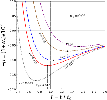
(a) $-\mu(t)$ vs $t/t_{{}_{0}}$ for ${\sigma_{\!{}_{0}}}=0.05$ and ${\mu_{{}_{0}}}\in(0,0.15)$.

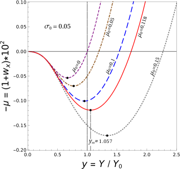
(b) $-\mu(t)$ vs $Y/Y_{\!{}_{0}}$ for ${\sigma_{\!{}_{0}}}=0.05$ and ${\mu_{{}_{0}}}\in(0,0.15)$.

Figure 1: Variation of the percentage correction in the effective dark energy EoS, viz. $-\mu=100(1+\mathsf{w}_{\!{}_{X}})$, with (a) the rationalized cosmic time $\tau=t/t_{{}_{0}}$, and (b) the rationalized correction $y=Y/Y_{\!{}_{0}}$ in the effective potential, for a fixed parametric value ${\sigma_{\!{}_{0}}}=0.05$, and discrete values of the parameter ${\mu_{{}_{0}}}$ in the range $(0,0.15)$. The thick dots indicate the minima of the plots.

I. For a fixed ${\sigma_{\!{}_{0}}}$, the requisite parametric range of ${\mu_{{}_{0}}}$ that meets the criterion $\,t_{{}_{C}}\in\left(t_{{}_{T}},t_{{}_{0}}\right)\,$ is by no means broad, especially given the condition that ${\sigma_{\!{}_{0}}}$ has to be small in order to make the linear approximation tenable. In particular, even if we consider fixing ${\sigma_{\!{}_{0}}}$ at a reasonably significant value $\,0.05$, the plots of the percentage correction $-\mu(\tau)$ [cf. Eq. (4.18)] in Fig. 1 (a), for various parametric values of ${\mu_{{}_{0}}}$, make it evident that the latter cannot go much further beyond $0.1$. Otherwise (for e.g. when ${\mu_{{}_{0}}}=0.15$), $t_{{}_{C}}$ would fall below $t_{{}_{T}}$, thus making the phantom crossing unrealistic. Analytically, this can be easily seen from Eq. (4.26), since with $\,\zeta_{{}_{0}}=1.1881\,$ and $\,t_{{}_{T}}=0.554\,t_{{}_{0}}\,$ [cf. Eqs. (4.22) and (4.24) respectively], the criterion $\,t_{{}_{C}}\in\left(t_{{}_{T}},t_{{}_{0}}\right)\,$ implies

$$0<\,{\mu_{{}_{0}}}\,\lesssim\,2.367\,{\sigma_{\!{}_{0}}}\,\left(=\,0.118\,,\,\,\mbox{for}\,\,{\sigma_{\!{}_{0}}}=0.05\right)\,.$$ (4.27)

The solid curve in Fig. 1 (a) shows the $\,-\mu(\tau)$ variation for the optimum value ${\mu_{{}_{0}}}=0.118$. The minimum point (or turning point) of this curve, at $\,\tau=\tau_{m}=0.945$, is of particular significance since it marks the earliest possible occurence of the minimum of $\,-\mu(\tau)$ corresponding to a ${\mu_{{}_{0}}}$ value legitimate for a realistic phantom crossing. More specifically, at the crossing point $\tau=\tau_{{}_{C}}$ the function $\,-\mu(\tau)$ requires to be decreasing at such a rate that the minimum point is reached very close to the present epoch, or afterwards. This is in fact a general requirement, irrespective of the chosen fixed value ${\sigma_{\!{}_{0}}}=0.05$, as verified below.

From Eqs. (4.18) and (4.19) we see that the minimization of $\,-\mu(\tau)$ implies that of $\mathsf{w}_{\!{}_{X}}^{(1)}(\tau)$. Therefore, using Eqs. (4.10) and (4.14), followed by (4.16) and (4.20), one obtains

$$\frac{\tanh(\zeta_{{}_{0}}\tau_{m})}{2\,\zeta_{{}_{0}}\tau_{m}} = -\,16\,\tau_{m}\,\mathsf{w}_{\!{}_{X}}^{(1)}(\tau_{m})$$ (4.28)

$$\approx \frac{\zeta_{{}_{0}}\tau_{m}}{\sinh^{2}(\zeta_{{}_{0}}\tau_{m})}\left[\left(1+\,\frac{4{\mu_{{}_{0}}}}{25{\sigma_{\!{}_{0}}}}\right)\frac{\sinh^{2}\zeta_{{}_{0}}}{\zeta_{{}_{0}}}+\,\mbox{Shi}(2\zeta_{{}_{0}}\tau_{m})-\,\mbox{Shi}(2\zeta_{{}_{0}})\right]-\,1\,\,,$$

or, equivalently, by virtue of the relationship (4.26),

$$\left[1+\,\frac{\tanh(\zeta_{{}_{0}}\tau_{m})}{2\,\zeta_{{}_{0}}\tau_{m}}\right]\frac{\sinh^{2}(\zeta_{{}_{0}}\tau_{m})}{\zeta_{{}_{0}}\tau_{m}}-\,\mbox{Shi}(2\zeta_{{}_{0}}\tau_{m})\approx\,\frac{\sinh^{2}(\zeta_{{}_{0}}\tau_{{}_{C}})}{\zeta_{{}_{0}}\tau_{{}_{C}}}-\,\mbox{Shi}(2\zeta_{{}_{0}}\tau_{{}_{C}})\,.$$ (4.29)

Solving this equation numerically, for $\zeta_{{}_{0}}=1.1881$, we get $\,\tau_{m}=0.945$ in the optimal case $\tau_{{}_{C}}=\tau_{{}_{T}}=0.554$ (or equivalently ${\mu_{{}_{0}}}=2.367\,{\sigma_{\!{}_{0}}}\,$), without any allusion to the typical fixation of ${\mu_{{}_{0}}}$ or ${\sigma_{\!{}_{0}}}$.

It is also worth examining how the percentage correction $\,-\mu(\tau)$ varies with the quantity $\,y(t)\equiv{}^{\displaystyle Y(t)\!}\!\!\!\diagup_{\!\!\displaystyle Y_{\!{}_{0}}}\,$, where $\,Y_{\!{}_{0}}\equiv Y(t_{{}_{0}})\,$ — the present-day value of the fractional correction in the potential, whose specific form, given by Eq. (4.4), makes the cosmic super-acceleration plausible. As we see from Fig. 1 (b), the criterion $\,t_{{}_{C}}\in\left(t_{{}_{T}},t_{{}_{0}}\right)\,$, and correspondingly the viable range of ${\mu_{{}_{0}}}$ (for a fixed ${\sigma_{\!{}_{0}}}$), could be ascribed to the valid zone of occurence of $y=y_{m}\,$ — the point at which $-\mu$ is minimized. In particular, the above bound ${\mu_{{}_{0}}}\lesssim 2.367\,{\sigma_{\!{}_{0}}}\,$ holds only for $\,y_{m}\lesssim 1.05\,$, thus implying that the $-\mu(y)$ variation should be such that the minimum point (or turning point) $y_{m}$ is reached later than almost the present epoch. This is a general condition for the viability of the phantom crossing, not just specific to the choice ${\sigma_{\!{}_{0}}}=0.05$. Fig. 1 (b) further illustrates that the phantom regime is non-transient, i.e. the super-acceleration is ever-lasting (despite slowing down progressively after the minimum point $y_{m}$ is reached). Analytically, this can be attributed to the fact that Eq. (4.4) implies the function $y$ to be approximately equal to $\tau^{-1}$. Therefore, in the asymptotic limit ($\tau\rightarrow\infty$), $y$ tends to vanish, and so does the correction $\mu$.

II. If, on the other hand, we resort to a fixed value of ${\mu_{{}_{0}}}$, say a fairly low one ($=0.05$), then as illustrated in Fig. 2 (a), and as derived from Eq. (4.26), a realistic phantom barrier crossing requires a lower limit on the parameter ${\sigma_{\!{}_{0}}}$, close to (but greater than) $0.02$, for the $\zeta_{{}_{0}}$ and $\tau_{{}_{T}}$ estimated above.

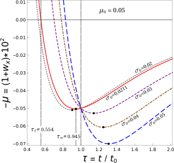
(a) $-\mu(t)$ vs $t/t_{{}_{0}}$ for ${\mu_{{}_{0}}}=0.05$ and ${\sigma_{\!{}_{0}}}\in(0.02,0.06)$.

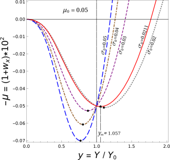
(b) $-\mu(t)$ vs $Y/Y_{\!{}_{0}}$ for ${\mu_{{}_{0}}}=0.05$ and ${\sigma_{\!{}_{0}}}\in(0.02,0.06)$.

Figure 2: Variation of the percentage correction in the effective dark energy EoS, viz. $-\mu=100(1+\mathsf{w}_{\!{}_{X}})$, with (a) the rationalized cosmic time $\tau=t/t_{{}_{0}}$, and (b) the rationalized correction $y=Y/Y_{\!{}_{0}}$ in the effective potential, for a fixed parametric value ${\mu_{{}_{0}}}=0.05$, and discrete values of the parameter ${\sigma_{\!{}_{0}}}$ in the range $(0.02,0.05)$. The thick dots indicate the minima of the plots.

However, if we aspire to get a much larger ${\mu_{{}_{0}}}$, say $\sim 0.5$ (i.e. about $\mfrac 12\%$ correction in $\mathsf{w}_{\!{}_{X}}$), then by Eq. (4.26), we require ${\sigma_{\!{}_{0}}}\gtrsim 0.211$, which may nonetheless compel us to go beyond the linear approximation. The above arguments regarding correlating the criterion $\,t_{{}_{C}}\in\left(t_{{}_{T}},t_{{}_{0}}\right)\,$ to the domain of appearance of the turning points $\tau=\tau_{m}$ would apply here as well. Also for completeness, it is worth examining the variation of $-\mu$ with $y={}^{\displaystyle Y\!}\!\!\!\diagup_{\!\!\displaystyle Y_{\!{}_{0}}}$, for ${\mu_{{}_{0}}}$ fixed at $0.05$ and various parametric values of ${\sigma_{\!{}_{0}}}$. The corresponding plots shown in Fig. 2 (b) display the same non-transient aspect of the phantom regime as illustrated in Fig. 1 (b) above.

5 Evolving Torsion parameters and the extent of the Super-acceleration

Let us recall the expressions (2.12) for the relevant (non-vanishing) torsion parameters, viz. the norms of the torsion mode vectors $\mathcal{T}_{\mu}$ and $\mathcal{A}_{\mu}$. With the quadratic MMT coupling function $\beta(\phi)$, given by Eq. (2.13), and the identification $\,s\gamma^{2}=\phi\equiv t$, such expressions reduce to

$$\mathcal{T}^{2}\equiv\,-g^{\mu\nu}\mathcal{T}_{\mu}\mathcal{T}_{\nu}=\,\frac{9}{t^{2}}\left[1-\frac{s}{4(t+s))}\right]^{2}\qquad\mbox{and}\qquad\mathcal{A}^{2}\equiv\,-g^{\mu\nu}\mathcal{A}_{\mu}\mathcal{A}_{\nu}=\,\frac{9s}{t(t+s)^{2}}\,\,.$$ (5.1)

Our interest, of course, is in getting a quantitative measure of the extent to which the scenario in Paper 1 is modified when the parameter $s\neq 0$. For this we require a careful examination of the time-evolution of

$$U_{T}:=\,\frac{\mathcal{T}^{2}-\overline{\mathcal{T}}^{2}}{\overline{\mathcal{T}}^{2}}\qquad\mbox{and}\qquad U_{A}:=\,\frac{\mathcal{A}^{2}}{\overline{\mathcal{T}}^{2}}\,\,,$$ (5.2)

which are the fractional changes over the only existent torsion parameter in Paper 1, viz.

$$\overline{\mathcal{T}}^{2}\equiv\Big{[}-g^{\mu\nu}\mathcal{T}_{\mu}\mathcal{T}_{\nu}\Big{]}_{s=0}=\,\frac{9}{t^{2}}\,\,,$$ (5.3)

that leads to the $\Lambda$CDM solution therein [189].

Using Eqs. (5.1) and (5.3), along with the definitions (4.2), we can write

$$U_{T}(\tau)=\,-\,\frac{U_{A}(\tau)}{2}\left(1+\frac{7{\sigma_{\!{}_{0}}}}{8\tau}\right)\,,\qquad U_{A}(\tau)=\,\frac{{\sigma_{\!{}_{0}}}\tau}{(\tau+{\sigma_{\!{}_{0}}})^{2}}\,\,,$$ (5.4)

and consequently re-express the fractional modification of the effective potential ($\overline{W}=2\Lambda$) of Paper 1 as

$$Y(\tau)=\,\frac{{\sigma_{\!{}_{0}}}}{16\left(\tau+{\sigma_{\!{}_{0}}}\right)}=\,-\,\frac{U_{A}(\tau)+\,16\,U_{T}(\tau)}{112}\,\,.$$ (5.5)

Note that so far we have not dealt with any approximation — the relations (5.4) and (5.5) are exact. Nevertheless, from the perspective of our analysis in the previous section (focusing per se, only on mild deviations from $\Lambda$CDM via the MMT extension), we shall only consider small values of the parameter ${\sigma_{\!{}_{0}}}$ from here on.

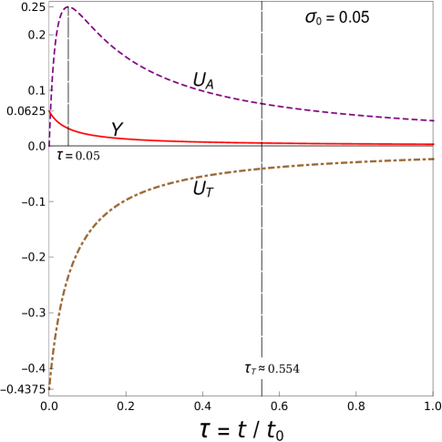
(a) $U_{A}$, $U_{T}$ and $Y$ vs $t/t_{{}_{0}}$ for ${\sigma_{\!{}_{0}}}=0.05$.

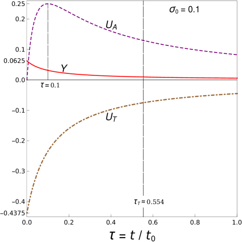
(b) $U_{A}$, $U_{T}$ and $Y$ vs $t/t_{{}_{0}}$ for ${\sigma_{\!{}_{0}}}=0.1$.

Figure 3: Variations of the fractional changes in the torsion parameters, viz. $U_{A}(\tau)$ and $U_{T}(\tau)$, and their resultant $Y(\tau)$, for fixed parametric values: (a) ${\sigma_{\!{}_{0}}}=0.05$ and (b) ${\sigma_{\!{}_{0}}}=0.1$.

Now for small ${\sigma_{\!{}_{0}}}$, the fractional corrections $U_{A}$ and $U_{T}$, albeit decreasing with time, remain of the same order of magnitude as ${\sigma_{\!{}_{0}}}$ itself, in the temporal range of interest $\,t\in(t_{{}_{T}},t_{{}_{0}})\,$, or equivalently $\,\tau\in(\tau_{{}_{T}},1)$. However, the resulting fractional change in the potential, $Y$, turns out be comparatively much smaller, as illustrated with two fiducial settings ${\sigma_{\!{}_{0}}}=0.05$ and ${\sigma_{\!{}_{0}}}=0.1$ in Figs. 3 (a) and (b) respectively.

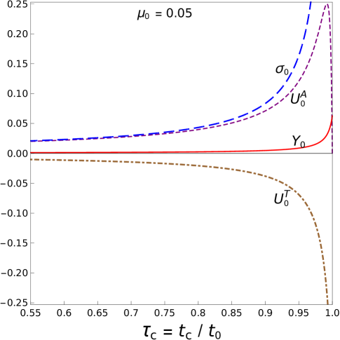
(a) ${\sigma_{\!{}_{0}}}$, $U^{A}_{\!{}_{0}}$, $U^{T}_{\!{}_{0}}$ and $Y_{\!{}_{0}}$ vs $t_{{}_{C}}/t_{{}_{0}}$ for ${\mu_{{}_{0}}}=0.05$.

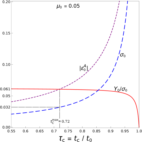
(b) ${\sigma_{\!{}_{0}}}$, $Y_{\!{}_{0}}/{\sigma_{\!{}_{0}}}$ and $|\varepsilon^{A}_{\!{}_{0}}|$ vs $t_{{}_{C}}/t_{{}_{0}}$ for ${\mu_{{}_{0}}}=0.05$.

Figure 4: Approximated variations of the parametric values of (a) ${\sigma_{\!{}_{0}}}$ and the fractional changes in the torsion parameters at the present epoch, viz. $U^{A}_{\!{}_{0}}$ and $U^{T}_{\!{}_{0}}$, as well as their resultant $Y_{\!{}_{0}}$, and (b) ${\sigma_{\!{}_{0}}}$, $Y_{\!{}_{0}}/{\sigma_{\!{}_{0}}}$, as well as the fractional deviation of $U^{A}_{\!{}_{0}}$ from ${\sigma_{\!{}_{0}}}$, with the rationalized phantom crossing time $\tau_{{}_{C}}=t_{{}_{C}}/t_{{}_{0}}$ in the viable range $(0.55,1)$, for a fixed ${\mu_{{}_{0}}}=0.05$.

This smallness of $Y$, and as a consequence the weak time-variation of the effective dark energy EoS $\mathsf{w}_{\!{}_{X}}$, of course justifies the linear approximation in the preceding section. Note also that the peak values of $U_{A},|U_{T}|$ and $Y$ are independent of the value of ${\sigma_{\!{}_{0}}}$. In particular, the above expression for $U_{A}$ implies that the latter attains its maximum value $\,(=0.25)$ at $\,\tau={\sigma_{\!{}_{0}}}$, as illustrated in Figs. 3 (a) and (b). On the other hand, $|U_{T}|$ and $Y$ being monotonically decreasing functions of $\tau$, have their maximum values (equal to $0.4375$ and $0.0625$ respectively) at $\tau=0$.

As to the values of $U_{A}$, $|U_{T}|$ and $Y$ at the present epoch $t=t_{{}_{0}}$, it is evident from Eqs. (5.4) and (5.5) that all of them are smaller than ${\sigma_{\!{}_{0}}}$, for $\,0<{\sigma_{\!{}_{0}}}\lesssim 1\,$:

$$U^{A}_{\!{}_{0}}\equiv\,U_{A}(t_{{}_{0}})=\,{\sigma_{\!{}_{0}}}\Big{[}1+\,\varepsilon^{A}_{\!{}_{0}}\Big{]}\,;\quad \quad\varepsilon^{A}_{\!{}_{0}}=\,-\,\frac{{\sigma_{\!{}_{0}}}\left(2+{\sigma_{\!{}_{0}}}\right)}{(1+{\sigma_{\!{}_{0}}})^{2}}=\,-\,2{\sigma_{\!{}_{0}}}+\mathcal{O}({\sigma_{\!{}_{0}}}^{2})\,\,,$$ with (5.6)

$$\left|U^{T}_{\!{}_{0}}\right|\equiv\,|U_{T}(t_{{}_{0}})|=\,\frac{{\sigma_{\!{}_{0}}}}{2}\Big{[}1+\,\varepsilon^{T}_{\!{}_{0}}\Big{]}\,;\quad \quad\varepsilon^{T}_{\!{}_{0}}=\,-\,\frac{{\sigma_{\!{}_{0}}}\left(9+8{\sigma_{\!{}_{0}}}\right)}{8(1+{\sigma_{\!{}_{0}}})^{2}}=\,-\,\frac{9{\sigma_{\!{}_{0}}}}{8}+\mathcal{O}({\sigma_{\!{}_{0}}}^{2})\,\,,$$ with (5.7)

$$Y_{\!{}_{0}}\equiv\,Y(t_{{}_{0}})=\,\frac{{\sigma_{\!{}_{0}}}}{16}\Big{[}1+\,\varepsilon^{Y}_{\!{}_{0}}\Big{]}\,;\quad \quad\varepsilon^{Y}_{\!{}_{0}}=\,-\,\frac{{\sigma_{\!{}_{0}}}}{1+{\sigma_{\!{}_{0}}}}=\,-\,{\sigma_{\!{}_{0}}}+\mathcal{O}({\sigma_{\!{}_{0}}}^{2})\,\,.$$ with (5.8)

Now, using Eq. (4.26) one can determine how ${\sigma_{\!{}_{0}}}$, and hence $\,U^{A}_{\!{}_{0}},\,|U^{T}_{\!{}_{0}}|$ and $Y_{\!{}_{0}}$, vary approximately with the rationalized phantom crossing time $\tau_{{}_{C}}\,(={}^{\displaystyle t_{{}_{C}}}\!\!\!\diagup_{\!\!\displaystyle t_{{}_{0}}})$, for a fixed value of the percentage correction ${\mu_{{}_{0}}}$ in $\mathsf{w}_{\!{}_{X}}$ at $t=t_{{}_{0}}$ (or $\tau=1$). Fig. 4 (a) shows such parametric variations, within the viable range $t_{{}_{C}}\in(t_{{}_{T}},t_{{}_{0}})$, or $\tau_{{}_{C}}\in(0.55,1)$, for a fiducial setting ${\mu_{{}_{0}}}=0.05$ (which nonetheless is well within the $1\sigma$ error estimates from recent observations [228]). A stringent upper limit can in principle be placed on $t_{{}_{C}}$, and hence on ${\sigma_{\!{}_{0}}}$, for a given value of ${\mu_{{}_{0}}}$, from the argument that $Y_{\!{}_{0}}$ would be of significance only when it is $\gtrsim{\sigma_{\!{}_{0}}}|\varepsilon^{A}_{\!{}_{0}}|$, where $|\varepsilon^{A}_{\!{}_{0}}|$ is the absolute fractional deviation of $U^{A}_{\!{}_{0}}$ from ${\sigma_{\!{}_{0}}}$. Specifically, this could be seen as a consequence of a stringent limit being imposed on the extent of the linear approximation, for which $U^{A}_{\!{}_{0}}\approx{\sigma_{\!{}_{0}}}$, by Eq. (5.6). The higher order change, i.e. the deviation of the exact $U^{A}_{\!{}_{0}}$ from ${\sigma_{\!{}_{0}}}$, given by the amount ${\sigma_{\!{}_{0}}}|\varepsilon^{A}_{\!{}_{0}}|$, need to be $\,\lesssim Y_{\!{}_{0}}$, because otherwise $Y_{\!{}_{0}}$ would also be a higher order effect, which would in turn imply the invalidity of the linear approximation. As shown in Fig. 4 (b), the effect of $Y_{\!{}_{0}}$ of a very small amount ($\lesssim 0.061{\sigma_{\!{}_{0}}}$), could yet be perceptible in the linear approximation (i.e. satisfy the condition $Y_{\!{}_{0}}\gtrsim{\sigma_{\!{}_{0}}}|\varepsilon^{A}_{\!{}_{0}}|\,$) and lead to a reasonably significant amount of ${\mu_{{}_{0}}}\,(=0.05)$, only if $t_{{}_{C}}\lesssim 0.72t_{{}_{0}}$, or ${\sigma_{\!{}_{0}}}\lesssim 0.032$ correspondingly. In principle, a lesser upper bound on ${\sigma_{\!{}_{0}}}$, culminating to an even smaller amount of $Y_{\!{}_{0}}$, may provide a more significant ${\mu_{{}_{0}}}$, however at the expense of reducing the upper limit of $t_{{}_{C}}$. One can therefore infer the following:

• As the phantom crossing time $t_{{}_{C}}$ cannot be smaller than the deceleration-to-acceleration transition time $t_{{}_{T}}$, the percentage correction ${\mu_{{}_{0}}}$ (in the effective DE equation of state $\mathsf{w}_{\!{}_{X}}(t_{{}_{0}})$) cannot get enhanced much further beyond the value $0.05$, at least in the linear approximation.

• Nevertheless, the extended MMT-cosmological scenario seems more attractive for a $t_{{}_{C}}$ value closer to $t_{{}_{T}}$, i.e. for an earlier commencement of the super-accelerating regime, from the point of view of having larger value of ${\mu_{{}_{0}}}$ with lesser strength of coupling ${\sigma_{\!{}_{0}}}$ of the mimetic field with the Holst term. In other words, the more weak the MMT extension, the more prominent is the effect in $\mathsf{w}_{\!{}_{X}}(t_{{}_{0}})$. There is a limit to this of course, since $t_{{}_{C}}$ must not fall short of $t_{{}_{T}}$.

6 Conclusion

A viable phantom crossing evolution of a unified cosmological dark sector is thus demonstrated by extending the basic mimetic-metric-torsion (MMT) formalism with an explicit coupling of the mimetic field $\phi$ and the Holst term, motivated from the following:

Firstly, its compliance with the basic precept of MMT gravity, viz. preservation of conformal symmetry while letting $\phi$ to manifest geometrically as the source of torsion (or certain mode(s) thereof).

Secondly, and most crucially, its instrumentality in making torsion’s main characteristic, viz. the anti-symmetry, accountable for the dynamical evolution of a given physical system.

To be more specific, the reason why we have incorporated the $\phi$-coupled Holst term is that, apart from keeping the conformal symmetry of the MMT theory unaffected, it ideally befits our objective of perceiving a plausible effect of the axial (or pseudo-trace) mode $\mathcal{A}_{\mu}$ of torsion, over and above the influence of the latter’s trace mode $\mathcal{T}_{\mu}$, on the cosmic evolution profile. In particular, for clarity in interpreting results, irrespective of the explicit $\phi$-coupling, we have preferred to resort to a non-topological characterization of the bare Holst term by promoting its coefficient, viz. the Barbero-Immirzi (BI) parameter $\gamma$, to the status of a field. Considering this field to be a (presumably primordial) pseudo-scalar (or, an axion), we could avoid gravitational parity violation, and hence a direct confrontation with the latter’s miniscule observational signature at cosmological scales. Consequently, an identification of $\phi$ with $\gamma^{2}$ (i.e. the simplest possible even function of $\gamma$), using a scalar Lagrange multiplier field, had made it evident that both the (a priori independent) torsion modes $\mathcal{T}_{\mu}$ and $\mathcal{A}_{\mu}$ are induced by $\phi$. In the paradigm of the standard FRW cosmology, the outcome is in some sense, a ‘geometric unification’ of the dark sector, as both the effective DM and DE components of the universe, being purportedly the artefacts of $\mathcal{T}_{\mu}$ and $\mathcal{A}_{\mu}$, have had their dynamics driven by the same scalar field $\phi$.

Technically of course, the MMT theory (introduced in Paper 1) is designed to have almost all of its weight resting on our consideration of a pre-assigned contact coupling, $\,\beta(\phi)$, between the mimetic field and the entire torsion-dependent part of the Riemann-Cartan ($U_{4}$) Lagrangian. In the extended formulation, such a coupling obviously carries to the Holst term, which augments the $U_{4}$ Lagrangian. The further postulation of a pseudo-scalar BI field, and subsequently the identification $\phi=s\gamma^{2}$ (where $s$ is a dimensionless constant), are only expected to lead to a subtle modification of what $\,\beta(\phi)$ alone can inflict on a given system configuration. Nevertheless, there arises the important question as to whether such a modification, despite its suppressed quantitativeness, can turn out to be of significance in the cosmological context. This is what we have addressed specifically via our analysis in the preceding sections.

In particular, taking the MMT coupling function in the form $\,\beta(\phi)\sim\phi^{2}\,$, we have brought the time-variance of the effective mimetic potential $W(\phi)$ in the reckoning, as opposed to its constancy in Paper 1, viz. $W=\overline{W}=2\Lambda$, due to the only existent torsion mode $\mathcal{T}_{\mu}$ (in absence of the Holst term) therein. While the coupling $\,\beta(\phi)\sim\phi^{2}\,$ has had its motivation from the point of view of its natural appearance in metric-torsion theories involving scalar field(s) [94, 145, 146, 147], the effect of the typical functional form it ascribes to the fractional modification $Y(\phi)$ of the constant potential $\overline{W}=2\Lambda$ (of Paper 1) has turned out to be quite fascinating in the cosmological context. Specifically, such a $\phi^{2}$-coupling implies an inverse functional dependence of $Y$ on $\phi$, or equivalently, on the cosmic time $t$ in the FRW framework. The consequence of this, by virtue of the mimetic constraint, is a super-accelerating phase of cosmic evolution, marked by the diminution of the effective DE equation of state parameter $\mathsf{w}_{\!{}_{X}}(t)$ below the value $-1$ (that corresponds to the $\Lambda$CDM model). In fact, as we have inferred via a set of arguments, the super-acceleration is always admissible in our extended MMT scenario, which most importantly, does not appear to have any theoretical obstacle(s), such as those concerning ghost or phantom degree(s) of freedom often faced in super-accelerating DE models. This may be understood from the point of view that none of the energy conditions, except the strong one, is violated in our entire formalism. The violation of the strong energy condition is of course nothing unusual — it is actually mandated for any attempt of explaining the late-time cosmic acceleration (regardless of an even later super-acceleration) in the standard FRW framework.

Nevertheless, despite having the theoretical consistency, there remained the task for us to assert whether the transition from $\mathsf{w}_{\!{}_{X}}>-1$ to $\mathsf{w}_{\!{}_{X}}<-1$, or the phantom barrier crossing, is at all physically realizable, and if so, under what condition(s). In specific terms, a physically realistic (or viable) phantom crossing implies that the epoch of its occurence, $t=t_{{}_{C}}$, has to be within the time-span $(t_{{}_{T}},t_{{}_{0}})$, where $t_{{}_{T}}$ denotes the deceleration-to-acceleration transition epoch and $t_{{}_{0}}$ denotes the present epoch. While the lower bound $t_{{}_{C}}>t_{{}_{T}}$ is obvious, the upper bound $t_{{}_{C}}<t_{{}_{0}}$ actually pertains to a fair amount of observational signification of a mild super-acceleration to have commenced in the near past phase of evolution of the universe, and continuing to the present epoch and beyond [228]. The mildness of course alludes to the gross observational concordance on $\Lambda$CDM cosmology. That is to say, in whichever way the DE equation of state parameter $\mathsf{w}_{\!{}_{X}}$ may deviate from the $\Lambda$CDM value $-1$, observations disfavour the latter’s error limits to be breached to any perceivable extent. Now, to determine the condition(s) for $t_{{}_{C}}\in(t_{{}_{T}},t_{{}_{0}})$ to hold (if at all), it is imperative to obtain the functional form of $\mathsf{w}_{\!{}_{X}}(t)$ by explicitly solving the corresponding cosmological equations. However, instead of attempting an exact analytic solution, we have adopted an approximation method, upon treating the effect of the function $Y(\phi)$ as a small perturbation over that due to the constant potential $\overline{W}=2\Lambda$, viz. the $\Lambda$CDM solution in Paper 1. Admittedly, the strong observational support for $\Lambda$CDM has made it reasonable for us to work in that way, i.e. to assume that $Y(\phi)$ would always inflict a small deviation of $\mathsf{w}_{\!{}_{X}}$ from the value $-1$.

Working out $\mathsf{w}_{\!{}_{X}}(t)$ in the approximated form, we have shown that the phantom crossing is indeed physically realizable, however for a severely restricted range of values of our MMT model parameters, viz. ${\sigma_{\!{}_{0}}}$ and ${\mu_{{}_{0}}}$, where $\,{\sigma_{\!{}_{0}}}={}^{\displaystyle s}\!\!\!\diagup_{\!\!\displaystyle t_{{}_{0}}}$ and ${\mu_{{}_{0}}}$ is the fractional amount by which $\mathsf{w}_{\!{}_{X}}$ differs from $-1$ at $t=t_{{}_{0}}$. In particular, limiting our analysis to the linear order of the (presumably small) parameter ${\sigma_{\!{}_{0}}}$, we have illustrated the time-evolution of $\mathsf{w}_{\!{}_{X}}$ for certain fiducial settings of either a fixed ${\sigma_{\!{}_{0}}}$ or a fixed ${\mu_{{}_{0}}}$. Strikingly enough, all such settings have made the revelation of the phantom regime being non-transient, i.e. the super-acceleration is ever-lasting, even though it slows down progressively after reaching an optimum point. A close inspection of the evolution profiles of the torsion parameters, viz. the norms of the torsion trace and pseudo-trace mode vectors $\mathcal{T}_{\mu}$ and $\mathcal{A}_{\mu}$, have enabled us to determine the validity of the linear approximation, and hence the extremity of the phantom crossing time $t_{{}_{C}}$, as well as that of $\mathsf{w}_{\!{}_{X}}(t_{{}_{0}})$ (or equivalently, ${\mu_{{}_{0}}}$). In fact, the latter is found to be not exceeding a value typically well within the combined Planck 2018 TT,TE,EE+lowE+Lensing+BAO error estimates for $\Lambda$CDM [228]. This nonetheless signifies a very low extent of the super-acceleration, in well accord with our presumption of its smallness.

On the whole, we have seen some really appealing outcomes of our entire program of extending the basic MMT formalism of Paper 1. Not only that it consolidates the tantalizing picture of a geometrically unified dark sector we have had therein, but also discerns a viable admittance of the cosmic super-acceleration, or the phantom phase, without any impending danger of dealing with a ghost-like entity. This may nonetheless be counted towards the robustness of the emergent cosmological model, since after all, from a purely theoretical standpoint, a provision for the phantom barrier crossing is desirable on account of the flexibility thus comprehended while making statistical estimations of the model parameters using the observational data. Nevertheless, apart from the technical difficulties the extreme mildness of the cosmic super-acceleration may pose in its detection with the current generation of observational probes, there remain several issues to be pondered on. For instance, (i) can there be any obvious way of realizing the $\phi$-coupling with torsion, with or without the involvement of the Holst term? (ii) would that be perceptible via the Hilbert-Palatini formulation of the mimetic gravity theory? (iii) how would the magnitude of the super-acceleration be affected if there be a constraint more complicated than (2.5)? (iv) can that constraint be imposed automatically (i.e. without the aid of a Lagrange multiplier) via some mechanism? (v) what is status of the gradient instability and how can we cope with that in the context of MMT gravity? Attempts of addressing to some of these are currently underway, and we hope to report them soon.

References

- [1] A. H. Chamseddine and V. Mukhanov, Mimetic Dark Matter, JHEP 1311 (2013) 135, [1308.5410].
- [2] A. H. Chamseddine, V. Mukhanov and A. Vikman, Cosmology with Mimetic Matter, JCAP 1406 (2014) 017, [1403.3961].
- [3] L. Sebastiani, S. Vagnozzi and R. Myrzakulov, Mimetic gravity: a review of recent developments and applications to cosmology and astrophysics, Adv. High Energy Phys. 2017 (2017) 3156915, [1612.08661].
- [4] E. A. Lim, I. Sawicki and A. Vikman, Dust of dark energy, JCAP 1005 (2010) 012, [1003.5751].
- [5] C. Gao, Y. Gong, X. Wang and X. Chen, Cosmological models with Lagrange multiplier field, Phys. Lett. B 702 (2011) no.2-3, 107, [1003.6056].
- [6] S. Capozziello, J. Matsumoto, S. Nojiri and S. D. Odintsov, Dark energy from modified gravity with Lagrange multipliers, Phys. Lett. B 693 (2010) no.2, 198, [1004.3691].
- [7] E. J. Copeland, M. Sami and S. Tsujikawa, Dynamics of dark energy, Int. J. Mod. Phys. D 15 (2006) 1753, [hep-th/0603057].
- [8] L. Amendola and S. Tsujikawa, Dark Energy: Theory and Observations, Cambridge University Press, United Kingdom (2010).
- [9] G. Wolschin, Lectures on Cosmology: Accelerated expansion of the Universe, Springer, Berlin, Heidelberg (2010).
- [10] S. Matarrese, M. Colpi, V. Gorini and U. Moschella, Dark Matter and Dark Energy: A Challenge for Modern Cosmology, Springer, The Netherlands (2011).
- [11] K. Bamba, S. Capozziello, S. Nojiri and S.D. Odintsov, Dark energy cosmology: the equivalent description via different theoretical models and cosmography tests, Astrophys. Space Sci. 342 (2012) 155, [1205.3421].
- [12] T. Chiba, gravity and scalar-tensor gravity, Phys. Lett. B 575 (2003) 1, [astro-ph/0307338].
- [13] S. Nojiri and S. D. Odintsov, Modified Gauss-Bonnet theory as gravitational alternative for dark energy, Phys. Lett. B 631 (2005) 1, [hep-th/0508049].
- [14] S. Nojiri and S. D. Odintsov, Modified gravity consistent with realistic cosmology: From matter dominated epoch to dark energy universe, Phys. Rev. D 74 (2006) 086005, [hep-th/0608008].
- [15] S. Nojiri and S. D. Odintsov, Introduction to modified gravity and gravitational alternative for dark energy, Int. J. Geom. Methods Mod. Phys. 04 (2007) 115, [hep-th/0601213].
- [16] S. Fay, R. Tavakol and S. Tsujikawa, gravity theories in Palatini formalism: Cosmological dynamics and observational constraints, Phys. Rev. D 75 (2007) 063509, [astro-ph/0701479].
- [17] T. P. Sotiriou and V. Faraoni, Theories of Gravity, Rev. Mod. Phys. 82 (2010) 451, [0805.1726].
- [18] A. De Felice and S. Tsujikawa, theories, Living Rev. Rel. 13 (2010) 3, [arXiv:1002.4928].
- [19] T. Clifton, P. G. Ferreira, A. Padilla and C. Skordis, Modified Gravity and Cosmology, Phys. Rept. 513 (2012) 1, [1106.2476].
- [20] E. Papantonopoulos, Modifications of Einstein’s Theory of Gravity at Large Distances, Lecture Notes in Physics, Springer, Switzerland (2015).
- [21] S. Nojiri, S. D. Odintsov and V. K. Oikonomou, Modified Gravity Theories on a Nutshell: Inflation, Bounce and Late-time Evolution, Phys. Rept. 692 (2017) 1, [1705.11098].
- [22] Y. Cai and Y.-S. Piao, Higher order derivative coupling to gravity and its cosmological implications, Phys. Rev. D 96 (2017) no.12, 124028, [1707.01017].
- [23] M. A. Gorji, S. A. H. Mansoori and H. Firouzjahi, Higher Derivative Mimetic Gravity, JCAP 1801 (2018) 020 [1709.09988].
- [24] M. Chaichian, J. Kluson, M. Oksanen and A. Tureanu, Mimetic dark matter, ghost instability and a mimetic tensor-vector-scalar gravity, JHEP 1412 (2014) 102, [1404.4008].
- [25] Y. Zheng, L. Shen, Y. Mou and M. Li, On (in)stabilities of perturbations in mimetic models with higher derivatives, JCAP 1708 (2017) 040, [1704.06834].
- [26] S. Hirano, S. Nishi and T. Kobayashi, Healthy imperfect dark matter from effective theory of mimetic cosmological perturbations, JCAP 1707 (2017) 009, [1704.06031].
- [27] K. Takahashi and T. Kobayashi, Extended mimetic gravity: Hamiltonian analysis and gradient instabilities, JCAP 1711 (2017) 038, [1708.02951].
- [28] J. Ben Achour, D. Langlois and K. Noui, Degenerate higher order scalar-tensor theories beyond Horndeski and disformal transformations, Phys. Rev. D 93 (2016) 124005, [1602.08398].
- [29] D. Langlois, M. Mancarella, K. Noui, F. Vernizzi, Mimetic gravity as DHOST theories, 1802.03394.
- [30] R. Myrzakulov and L. Sebastiani, Non-local - mimetic gravity, Astrophys. Space Sci. 361 (2016) 188, [1601.04994].
- [31] D. Momeni, R. Myrzakulov and E. Gudekli, Cosmological viable mimetic and theories via Noether symmetry, Int. J. Geom. Meth. Mod. Phys. 12 (2015) 1550101, [1502.00977].
- [32] A. V. Astashenok, S. D. Odintsov and V. K. Oikonomou, Modified Gauss-Bonnet gravity with the Lagrange multiplier constraint as mimetic theory, Class. Quant. Grav. 32 (2015) 185007, [1504.04861].
- [33] E. H. Baffou, M. J. S. Houndjo, M. Hamani-Daouda and F. G. Alvarenga, Late time cosmological approach in mimetic gravity, Eur. Phys. J. C 77 (2017) no.10, 708, [1706.08842].
- [34] F. Arroja, N. Bartolo, P. Karmakar and S. Matarrese, The two faces of mimetic Horndeski gravity: disformal transformations and Lagrange multiplier, JCAP 1509 (2015) 051, [1506.08575].
- [35] G. Cognola, R. Myrzakulov, L. Sebastiani, S. Vagnozzi and S. Zerbini, Covariant Horava-like and mimetic Horndeski gravity: cosmological solutions and perturbations, Class. Quant. Grav. 33 (2016) 225014, [1601.00102].
- [36] M. Bouhmadi-Lopez, C.-Y. Chen and P. Chen, Primordial Cosmology in Mimetic Born-Infeld Gravity, JCAP 1711 (2017) 053, [1709.09192].
- [37] C.-Y. Chen, M. Bouhmadi-Lopez and P. Chen, Black hole solutions in mimetic Born-Infeld gravity, Eur. Phys. J. C 78 (2018) no.1, 59, [1710.10638].
- [38] N. Sadeghnezhad and K. Nozari, Braneworld Mimetic Cosmology, Phys. Lett. B 769 (2017) 134, [1703.06269].
- [39] Y. Zhong, Y. Zhong, Y.-P. Zhang, Y.-X. Liu, Thick branes with inner structure in mimetic gravity, Eur. Phys. J. C 78 (2018) 45, [1711.09413].
- [40] Y. Zhong, Y.-P. Zhang, W.-D. Guo and Y.-X. Liu, Gravitational resonances in mimetic thick branes, JHEP 1904 (2019) 154, [1812.06453].
- [41] A. H. Chemseddine and V. Mukhanov, Ghost Free Mimetic Massive Gravity, JHEP 1806 (2018) 060, [1805.06283].
- [42] A. H. Chemseddine and V. Mukhanov, Mimetic Massive Gravity: Beyond Linear Approximation, JHEP 1806 (2018) 062, [1805.06598].
- [43] O. Malaeb and C. Saghir, Hamiltonian Formulation of Ghost Free Mimetic Massive Gravity, Eur. Phys. J. C 79 (2019) no.7, 584, [1901.06727].
- [44] A. R. Solomon, V. Vardanyan and Y. Akrami, Massive mimetic cosmology, Phys. Lett. B 794 (2019) 135, [1902.08533].
- [45] D. Momeni, A. Altaibayeva and R. Myrzakulov, New Modified Mimetic Gravity, Int. J. Geom. Meth. Mod. Phys. 11 (2014) 1450091, [1407.5662].
- [46] R. Myrzakulov, L. Sebastiani, S. Vagnozzi and S. Zerbini, Mimetic covariant renormalizable gravity, Fund. J. Mod. Phys. 8 (2015) 119–124, [1505.03115].
- [47] N. A. Koshelev, Effective dark matter fluid with higher derivative corrections, 1512.07097.
- [48] E. N. Saridakis and M. Tsoukalas, Bi-scalar modified gravity and cosmology with conformal invariance, JCAP 1604 (2016) 017, [1602.06890].
- [49] R. Kimura, A. Naruko and D. Yoshida, Extended vector-tensor theories, JCAP 1701 (2017) 002, [1608.07066].
- [50] M. A. Gorji, S. Mukohyama, H. Firouzjahi and S. A. Hosseini Mansoori, Gauge Field Mimetic Cosmology, JCAP 1808 (2018) no.08, 047, [1807.06335].
- [51] P. Jiroušek and A. Vikman, New Weyl-invariant vector-tensor theory for the cosmological constant, JCAP 1904 (2019) 004, [1811.09547].
- [52] A. H. Chamseddine, V. Mukhanov and T. B. Russ, Asymptotically Free Mimetic Gravity, Eur. Phys. J. C 79 (2019) No.7, 558, [1905.01343].
- [53] A. H. Chamseddine, V. Mukhanov and T. B. Russ, Mimetic Horava Gravity, Phys. Lett. B 798 (2019) 134939, [1908.01717].
- [54] O. Malaeb and C. Saghir, Mimetic Horava Gravity and Surface terms, 2005.02469.
- [55] A. O. Barvinsky, Dark matter as a ghost free conformal extension of Einstein’s theory, JCAP 1401 (2014) 014, [1311.3111].
- [56] K. Hammer and A. Vikman, Many Faces of Mimetic Gravity, 1512.09118.
- [57] M. Raza, K. Myrzakulov, D. Momeni and R. Myrzakulov, Mimetic Attractors, Int. J. Theor. Phys. 55 (2016) 2558, [1508.00971].
- [58] J. Dutta, W. Khyllep, E. N. Saridakis, N. Tamanini and S. Vagnozzi, Cosmological dynamics of mimetic gravity, JCAP 1802 (2018) 041, [1711.07290].
- [59] G. Leon and E. N. Saridakis, Dynamical behavior in mimetic gravity, JCAP 1504 (2015) 031, [1501.00488].
- [60] S. D. Odintsov and V. K. Oikonomou, Accelerating Cosmology and Phase Structure of Gravity with Lagrange Multiplier Constraint: Mimetic Approach, Phys. Rev. D 93 (2016) no.2, 023517, [1511.04559].
- [61] S. Nojiri and S. D. Odintsov, Mimetic gravity: inflation, dark energy and bounce, Mod. Phys. Lett. A 29 (2014) 1450211, [1408.3561].
- [62] S. Nojiri, S. D. Odintsov and V. K. Oikonomou, Viable Mimetic Completion of Unified Inflation-Dark Energy Evolution in Modified Gravity, Phys. Rev. D 94 (2016) no.10, 104050, [1608.07806].
- [63] R. Myrzakulov, L. Sebastiani and S. Vagnozzi, Inflation in - theories and mimetic gravity scenario, Eur. Phys. J. C 75 (2015) 444, [1504.07984].
- [64] S. D. Odintsov and V. K. Oikonomou, Unimodular Mimetic Inflation, Astrophys. Space Sci. 361 (2016) 236, [1602.05645].
- [65] S. D. Odintsov and V. K. Oikonomou, The reconstruction of and mimetic gravity from viable slow-roll inflation, Nucl. Phys. B 929 (2018) 79, [1801.10529].
- [66] A. H. Chamseddine and V. Mukhanov, Resolving Cosmological Singularities, JCAP 1703 (2017) 009, [1612.05860].
- [67] S. Brahma, A. Golovnev and D.-H. Yeom, On singularity-resolution in mimetic gravity, Phys. Lett. B 782 (2018) 280, [1803.03955].
- [68] J. De Haro, L. A. Saló and Supriya Pan, Limiting curvature mimetic gravity and its relation to Loop Quantum Cosmology , Gen. Rel. Grav. 51 (2019) no. 4, 49, [1803.09653].
- [69] R. Myrzakulov, L. Sebastiani, S. Vagnozzi and S. Zerbini, Static spherically symmetric solutions in mimetic gravity: rotation curves and wormholes, Class. Quant. Grav. 33 (2016) 125005, [1510.02284].
- [70] S. Vagnozzi, Recovering a MOND-like acceleration law in mimetic gravity, Class. Quant. Grav. 34 (2017) 185006, [1708.00603].
- [71] R. Myrzakulov and L. Sebastiani, Spherically symmetric static vacuum solutions in Mimetic gravity, Gen. Rel. Grav. 47 (2015) 89, [1503.04293].
- [72] D. Momeni, P. H. R. S. Moraes, H. Gholizade and R. Myrzakulov, Mimetic Compact Stars, Int. J. Geom. Meth. Mod. Phys. 15 (2018) no.06, 1850091, [1505.05113].
- [73] A. V. Astashenok and S. D. Odintsov, From neutron stars to quark stars in mimetic gravity, Phys. Rev. D 94 (2016) 063008, [1512.07279].
- [74] A. H. Chamseddine and V. Mukhanov, Nonsingular Black Hole, Eur. Phys. J. C 77 (2017) 183, [1612.05861].
- [75] G. G. L. Nashed, Spherically symmetric black hole solution in mimetic gravity and anti-evaporation, Int. J. Geom. Meth. Mod. Phys. 15 (2018) no.09, 1850154.
- [76] G. G. L. Nashed, W. El Hanafy and K. Bamba, Charged rotating black holes coupled with nonlinear electrodynamics Maxwell field in the mimetic gravity, JCAP 1901 (2019) no.01, 058, [1809.02289].
- [77] A. H. Chamseddine, V. Mukhanov and T. B. Russ, Black Hole Remnants, JHEP 10 (2019) 104, [1908.03498]
- [78] K. Hammer, P. Jirousek and A. Vikman, Axionic cosmological constant, 2001.03169.
- [79] J. Sakstein and B. Jain, Implications of the Neutron Star Merger GW170817 for Cosmological Scalar-Tensor Theories, Phys. Rev. Lett. 119 (2017) no.25, 251303, [1710.05893].
- [80] T. Baker, E. Bellini, P. G. Ferreira, M. Lagos, J. Noller and I. Sawicki, Strong constraints on cosmological gravity from GW170817 and GRB 170817A, Phys. Rev. Lett. 119 (2017) no.25, 251301, [1710.06394].
- [81] D. Langlois, R. Saito, D. Yamauchi and K. Noui, Scalar-tensor theories and modified gravity in the wake of GW170817, Phys. Rev. D 97 (2018) no.6, 061501, [1711.07403].
- [82] R. A. Battye, F. Pace and D. Trinh, Gravitational wave constraints on dark sector models, Phys. Rev. D 98 (2018) no.2, 023504, [1802.09447].
- [83] M. Rinaldi, L. Sebastiani, A. Casalino and S. Vagnozzi, Mimicking dark matter and dark energy in a mimetic model compatible with GW170817, Phys. Dark Univ. 22 (2018) 108, [1803.02620].
- [84] A. Ganz, N. Bartolo, P. Karmakar and S. Matarrese, Gravity in mimetic scalar-tensor theories after GW170817, JCAP 1901 (2019) no.01, 056, [1809.03496].
- [85] A. Casalino, M. Rinaldi, L. Sebastiani and S. Vagnozzi, Alive and well: mimetic gravity and a higher-order extension in light of GW170817, Class. Quant. Grav. 36 (2019) no.1, 017001, [1811.06830].
- [86] A. Einstein, The Meaning of Relativity: Fifth edition, including the RELATIVISTIC THEORY OF THE NON-SYMMETRIC FIELD, Princeton University Press, New Jersey, 1970.
- [87] A. Trautman, Spin and torsion may avert gravitational singularities, Nature 242 (1973) 7.
- [88] F. W. Hehl, P. Von Der Heyde, G. Kerlick and J. Nester, General Relativity with Spin and Torsion: Foundations and Prospects, Rev. Mod. Phys. 48 (1976) 393.
- [89] A. K. Raychaudhuri, Theoretical Cosmology, Clarendon Press, Oxford, United Kingdom (1979).
- [90] V. de Sabbata and M. Gasperini, Introduction to Gravitation, World Scientific, Singapore (1985).
- [91] V. de Sabbata and C. Sivaram, Spin Torsion and Gravitation, World Scientific, Singapore (1994).
- [92] F. W. Hehl, J. D. McCrea, E. W. Mielke and Y. Neéman, Metric affine gauge theory of gravity: Field equations, Noether identities, world spinors and breaking of dilation invariance, Phys. Rept. 258 (1995) 1, [gr-qc/9402012].
- [93] F. W. Hehl and Y. N. Obukhov, How does the electromagnetic field couple to gravity, in particular to metric, nonmetricity, torsion and curvature?, Lect. Notes Phys. 562 (2001) 479, [gr-qc/0001010].
- [94] I. L. Shapiro, Physical aspects of the space-time torsion, Phys. Rept. 357 (2002) 113, [hep-th/0103093].
- [95] M. Blagojevic, Gravitation and Gauge symmetries, IOP Publishing, London, United Kingdom (2002).
- [96] L. Fabbri, Higher-Order Theories of Gravitation, Ph.D. Thesis, 0806.2610.
- [97] S. Capozziello and M. De Laurentis, Extended Theories of Gravity, Phys. Rept. 509 (2011) 167, [1108.6266].
- [98] N. Poplawski, Affine theory of gravitation, Gen. Rel. Grav. 46 (2014) 1625, [1203.0294].
- [99] H. F. Westman and T. G. Zlosnik, An introduction to the physics of Cartan gravity, Annals Phys. 361 (2015) 330, [1411.1679].
- [100] J. A. Musante, Conformal Gauge Relativity: On the Geometrical Unification of Gravitation and Gauge Fields, 1008.2677.
- [101] L. Fabbri, Metric-Torsional Conformal Gravity, Phys. Lett. B 707 (2012) 415, [1101.1761].
- [102] D. R. Bergman, Internal Symmetry of Space-Time Connections with Torsion, 1411.5568.
- [103] P. Majumdar and S. SenGupta, Parity violating gravitational coupling of electromagnetic fields, Class. Quant. Grav. 16 (1999) L89, [gr-qc/9906027].
- [104] R. T. Hammond, Strings in gravity with torsion, Gen. Rel. Grav. 32 (2000) 2007, [gr-qc/9904033].
- [105] B. Mukhopadhyaya, S. Sen and S. SenGupta, Does a Randall-Sundrum scenario create the illusion of a torsion free universe?, Phys. Rev. Lett. 89 (2002) 121101 [Erratum ibid. 89 (2002) 259902], [hep-th/0204242].
- [106] S. Bhattacharjee and A. Chatterjee, Gauge invariant coupling of fields to torsion: a string inspired model, Phys. Rev. D 83 (2011) 106007, [1101.0118].
- [107] B. Mukhopadhyaya, S. Sen and S. SenGupta, A Randall-Sundrum scenario with bulk dilaton and torsion, Phys. Rev. D 79 (2009) 124029, [0903.0722].
- [108] R. Ferraro and F. Fiorini, Modified teleparallel gravity: Inflation without inflaton, Phys. Rev. D 75 (2007) 084031, [gr-qc/0610067].
- [109] G. R. Bengochea and R. Ferraro, Dark torsion as the cosmic speed-up, Phys. Rev. D 79, (2009) 124019, [0812.1205].
- [110] B. Li, T.P. Sotiriou and J. D. Barrow, Large-scale Structure in Gravity, Phys. Rev. D 83 (2011) 104017, [1103.2786].
- [111] Y.-F. Cai, S.-H. Chen, J. B. Dent, S. Dutta and E. N. Saridakis, Matter Bounce Cosmology with the Gravity, Class. Quant. Grav. 28 (2011) 215011, [1104.4349].
- [112] C. G. Böhmer, A. Mussa and N. Tamanini, Existence of relativistic stars in gravity, Class. Quant. Grav. 28 (2011) 245020, [1107.4455].
- [113] Y.-F. Cai, S. Capozziello, M. De Laurentis and E. N. Saridakis, teleparallel gravity and cosmology, Rept. Prog. Phys. 79 (2016) 106901, [1511.07586].
- [114] S. Bahamonde and C. G. Böhmer, Modified teleparallel theories of gravity: Gauss-Bonnet and trace extensions, Eur. Phys. J. C 76 (2016) no.10, 578, [1606.05557].
- [115] S. Bahamonde, S. Capozziello, M. Faizal and R. C. Nunes, Nonlocal Teleparallel Cosmology, Eur. Phys. J. C 77 (2017) no.9, 628, [1709.02692].
- [116] H.-J. Yo and J. M. Nester, Dynamic Scalar Torsion and an Oscillating Universe, Mod. Phys. Lett. A 22 (2007) 2057, [astro-ph/0612738].
- [117] A. V. Minkevich, A. S. Garkun and V. I. Kudin, Regular accelerating universe without dark energy, Class. Quant. Grav. 24 (2007) 5835, [0706.1157].
- [118] J. M. Nester, L. L. So and T. Vargas, On the energy of homogeneous cosmologies, Phys. Rev. D 78 (2008) 044035, [0803.0181].
- [119] P. Baekler, F. W. Hehl and J. M. Nester, Poincaré gauge theory of gravity: Friedmann cosmology with even and odd parity modes. Analytic part, Phys. Rev. D 83 (2011) 024001, [1009.5112].
- [120] C.-Q. Geng, C.-C. Lee and H.-H. Tseng, Scalar-Torsion Cosmology in the Poincaré Gauge Theory of Gravity, JCAP 1211 (2012) 013, [1207.0579].
- [121] M. Blagojevic and F. W. Hehl, Gauge Theories of Gravitation: A Reader with Commentaries, World Scientific, Singapore (2013).
- [122] J. Lu and G. Chee, Cosmology in Poincaré gauge gravity with a pseudoscalar torsion, JHEP 1605 (2016) 024, [1601.03943].
- [123] Y. N. Obukhov, Poincaré gauge gravity: An overview, Int. J. Geom. Meth. Mod. Phys. 15 (2018) no. supp.01, 1840005, [1805.07385].
- [124] S. Hojman, M. Rosenbaum and M.P. Ryan, Propagating torsion and gravitation, Phys. Rev. D 19 (1979) 430.
- [125] S.M. Carroll and G.B. Field, Consequences of propagating torsion in connection dynamic theories of gravity, Phys. Rev. D 50 (1994) 3867, [gr-qc/9403058].
- [126] A. Saa, Propagating torsion from first principles, Gen. Rel. Grav. 29 (1997) 205, [gr-qc/9609011].
- [127] A.S. Belyaev and I.L. Shapiro, The action for the (propagating) torsion and the limits on the torsion parameters from present experimental data, Phys. Lett. B 425 (1998) 246, [hep-ph/9712503].
- [128] N.J. Poplawski, Propagating torsion in the Einstein gauge, J. Math. Phys. 47 (2006) 112504, [gr-qc/0605061].
- [129] M. Blagojevic and B. Cvetkovic, Three-dimensional gravity with propagating torsion: Hamiltonian structure of the scalar sector, Phys. Rev. D 88 (2013) 104032, [1309.0411].
- [130] V. Nikiforova and T. Damour, Infrared modified gravity with propagating torsion: instability of torsionfull de Sitter-like solutions, Phys. Rev. D 97 (2018) no.12, 124014, [1804.09215].
- [131] G. Allemandi, M. Capone, S. Capozziello and M. Francaviglia, Conformal aspects of Palatini approach in extended theories of gravity, Gen. Rel. Grav. 38 (2006) 33, [hep-th/0409198].
- [132] V. Faraoni and S. Capozziello, Beyond Einstein Gravity: A Survey of Gravitational Theories for Cosmology and Astrophysics, Fundamental Theories of Physics 170 (2010), Dordrecht, Springer (2011).
- [133] D.A. Carranza, S. Mendoza and L.A. Torres, A cosmological dust model with extended gravity, Eur. Phys. J. C 73 (2013) 2282, [1208.2502].
- [134] F.W. Hehl, Yu. N. Obukhov, G.F. Rubilar and M. Blagojevic, On the theory of the skewon field: From electrodynamics to gravity, Phys. Lett. A 347 (2005) 14, [gr-qc/0506042].
- [135] J. B. Fonseca-Neto, C. Romero and S. P. G. Martinez, Scalar torsion and a new symmetry of general relativity, Gen. Rel. Grav. 45 (2013) 1579, [1211.1557].
- [136] S. Vignolo, L. Fabbri and C. Stornaiolo, A square-torsion modification of Einstein-Cartan theory, Annalen Phys. 524 (2012) 826, [1201.0286].
- [137] J.-A. Lu, theories of gravity without big-bang singularity, Annals Phys. 354 (2015) 424, [1404.4440].
- [138] L. Fabbri, A discussion on the most general torsion-gravity with electrodynamics for Dirac spinor matter fields, Int. J. Geom. Meth. Mod. Phys. 12 (2015) no. 09, 1550099, [1409.2007].
- [139] T. B. Vasilev, J. A. R. Cembranos, J. G. Valcarcel and P. Martín-Moruno, Stability in quadratic torsion theories, Eur. Phys. J. C 77 (2017) no. 11, 755, [1706.07080].
- [140] R. K. Kaul and S. Sengupta, Degenerate spacetimes in first order gravity, Phys. Rev. D 93 (2016) no.8, 084026, [1602.04559].
- [141] R. K. Kaul and S. Sengupta, New solutions in pure gravity with degenerate tetrads, Phys. Rev. D 94 (2016) no.10, 104047, [1609.02344].
- [142] S. Sengupta, Spacetime-bridge solutions in vacuum gravity, Phys. Rev. D 96 (2017) no.10, 104031, [1708.04971].
- [143] R. K. Kaul and S. Sengupta, Degenerate extension of the Schwarzschild exterior, Phys. Rev. D 96 (2017) no.10, 104011, [1709.00188].
- [144] S. Sengupta, Time travel in vacuum spacetimes, Phys. Rev. D 97 (2018) no.12, 124038, [1805.03035].
- [145] S. Sur and A. S. Bhatia, Weakly dynamic dark energy via metric-scalar couplings with torsion, JCAP 1707 (2017) 039, [1611.00654].
- [146] A. S. Bhatia and S. Sur, Phase Plane Analysis of Metric-Scalar Torsion Model for Interacting Dark Energy, 1611.06902.
- [147] A. S. Bhatia and S. Sur, Dynamical system analysis of dark energy models in scalar coupled metric-torsion theories, Int. J. Mod. Phys. D 26 (2017) no.13, 1750149, [1702.01267].
- [148] B. Mirza and F. Oboudiat, Mimetic Teleparallel gravity and cosmology, 1712.03363.
- [149] W.-D. Guo, Y. Zhong, K. Yang, T.-T. Sui and Y.-X. Liu, Thick brane in mimetic gravity, 1805.05650.
- [150] G.F. Rubilar, Y.N. Obukhov and F.W. Hehl, Torsion nonminimally coupled to the electromagnetic field and birefringence, Class. Quant. Grav. 20 (2003) L185, [gr-qc/0305049].
- [151] W.-T. Ni, Skewon field and cosmic wave propagation, Phys. Lett. A 378 (2014) 1217, [1312.3056].
- [152] S. SenGupta and S. Sur, Spherically symmetric solutions of gravitational field equations in Kalb-Ramond background, Phys. Lett. B 521 (2001) 350, [gr-qc/0102095].
- [153] S. SenGupta and A. Sinha, Fermion helicity flip in a Kalb-Ramond background, Phys. Lett. B 514 (2001) 109, [hep-th/0102073].
- [154] P. Das, P. Jain and S. Mukherji, Cosmic birefringence within the framework of heterotic string theory, Int. J. Mod. Phys. A 16 (2001) 4011, [hep-ph/0011279].
- [155] S. Kar, P. Majumdar, S. SenGupta and A. Sinha, Does a Kalb-Ramond field make space-time optically active?, Eur. Phys. J. C 23 (2002) 357, [gr-qc/0006097].
- [156] S. Kar, P. Majumdar, S. SenGupta and S. Sur, Cosmic optical activity from an inhomogeneous Kalb-Ramond field, Class. Quant. Grav. 19 (2002) 677, [hep-th/0109135].
- [157] S. Kar, S. SenGupta and S. Sur, Static spherisymmetric solutions, gravitational lensing and perihelion precession in Einstein-Kalb-Ramond theory, Phys. Rev. D 67 (2003) 044005, [hep-th/0210176].
- [158] S. SenGupta and S. Sur, Does curvature dilaton coupling with a Kalb-Ramond field lead to an accelerating universe?, JCAP 0312 (2003) 001, [hep-th/0207065].
- [159] D. Maity, S. SenGupta and S. Sur, Spinning test particle in Kalb-Ramond background, Eur. Phys. J. C 42 (2005) 453, [hep-th/0409143].
- [160] S. Sur, S. Das and S. SenGupta, Charged black holes in generalized dilaton-axion gravity, JHEP 0510 (2005) 064, [hep-th/0508150].
- [161] J. Alexandre, N. E. Mavromatos and D. Tanner, Non-perturbative time-dependent String Backgrounds and Axion-induced Optical Activity, Phys. Rev. D 78 (2008) 066001, [arXiv:0804.2353].
- [162] M. de Cesare, N. E. Mavromatos and S. Sarkar, On the possibility of tree-level leptogenesis from Kalb-Ramond torsion background, Eur. Phys. J. C 75 (2015) 514, [arXiv:1412.7077].
- [163] S. SenGupta and S. Sur, Gravitational Redshift in Einstein-Kalb-Ramond space-time and Randall-Sundrum scenario, Europhys. Lett. 65 (2004) 601, [hep-th/0306048].
- [164] D. Maity and S. SenGupta, Cosmic optical activity in a Randall-Sundrum brane world with bulk Kalb-Ramond field, Class. Quant. Grav. 21 (2004) 3379 [hep-th/0311142].
- [165] D. Maity, S. SenGupta and S. Sur, Observable signals in a string inspired axion-dilaton background and Randall-Sundrum scenario, Phys. Rev. D 72 (2005) 066012, [hep-th/0507210].
- [166] S. Das, A. Dey and S. SenGupta, Readdressing the hierarchy problem in a Randall-Sundrum scenario with bulk Kalb-Ramond background, Class. Quant. Grav. 23 (2006) L67, [hep-th/0511247].
- [167] A. Das, B. Mukhopadhyaya and S. SenGupta, Why has spacetime torsion such negligible effect on the Universe?, Phys. Rev. D 90 (2014) 107901, [1410.0814].
- [168] S. Chakraborty and S. SenGupta, Solutions on a brane in a bulk spacetime with Kalb-Ramond field, Annals Phys. 367 (2016) 258, [1412.7783].
- [169] S. Chakraborty and S. SenGupta, Strong gravitational lensing – A probe for extra dimensions and Kalb-Ramond field, JCAP 1707 (2017) no.07, 045, [1611.06936].
- [170] S. Chakraborty and S. SenGupta, Packing extra mass in compact stellar structures: An interplay between Kalb-Ramond field and extra dimensions, JCAP 1805 (2018) no.05, 032, [1708.08315].
- [171] C.-Q. Geng, C.-C. Lee, E. N. Saridakis and Y.-P. Wu, “Teleparallel” dark energy, Phys. Lett. B 704 (2011) 384, [1109.1092].
- [172] C.-Q. Geng, C.-C. Lee and E. N. Saridakis, Observational Constraints on Teleparallel Dark Energy, JCAP 1201 (2012) 002, [1110.0913].
- [173] L. Iorio and E. N. Saridakis, Solar system constraints on gravity, Mon. Not. Roy. Astron. Soc. 427 (2012) 1555, [1203.5781].
- [174] S. Capozziello, P. A. Gonzalez, E. N. Saridakis and Y. Vasquez, Exact charged black-hole solutions in -dimensional gravity: torsion vs curvature analysis, JHEP 1302 (2013) 039, [1210.1098].
- [175] M. A. Skugoreva, E. N. Saridakis and A. V. Toporensky, Dynamical features of scalar-torsion theories, Phys. Rev. D 91 (2015) 044023, [1412.1502].
- [176] G. Kofinas, E. Papantonopoulos and E. N. Saridakis, Self-Gravitating Spherically Symmetric Solutions in Scalar-Torsion Theories, Phys. Rev. D 91 (2015) 104034, [1501.00365].
- [177] S. Capozziello, O. Luongo, R. Pincak and A. Ravanpak, Cosmic acceleration in non-flat cosmology, Gen. Rel. Grav. 50 (2018) no.5, 53, [1804.03649].
- [178] G. Farrugia, J. Levi Said, V. Gakis and E. N. Saridakis, Gravitational Waves in Modified Teleparallel Theories, Phys. Rev. D 97 (2018) no.12, 124064, [1804.07365].
- [179] K.-F. Shie, J.M. Nester and H.-J. Yo, Torsion Cosmology and the Accelerating Universe, Phys. Rev. D 78 (2008) 023522, [0805.3834].
- [180] A. V. Minkevich, Accelerating Universe without dark energy and dark matter and spacetime torsion, Phys. Lett. B 678 (2009) 423, [0902.2860].
- [181] V. Nikiforova, S. Randjbar-Daemi and V. Rubakov, Self-accelerating Universe in modified gravity with dynamical torsion, Phys. Rev. D 95 (2017) no. 2, 024013, [1606.02565].
- [182] V. A. Kostelecky, N. Russell and J. Tasson, New Constraints on Torsion from Lorentz Violation, Phys. Rev. Lett. 100 (2008) 111102, [0712.4393].
- [183] E. E. Flanagan and E. Rosenthal, Can gravity probe B usefully constrain torsion gravity theories?, Phys. Rev. D 75 (2007) 124016, [0704.1447].
- [184] O. V. Babourova and B. N. Frolov, Interaction of the 4-rotational gauge field with orbital momentum, gravidiamagnetic effect and orbit experiment ‘Gravity Probe B’, Phys. Rev. D 82 (2010) 027503, [1004.1790].
- [185] F. W. Hehl, Y. N. Obukhov and D. Puetzfeld, On Poincaré gauge theory of gravity, its equations of motion and Gravity Probe B, Phys. Lett. A 377 (2013) 1775, [1304.2769].
- [186] S. Camera, V. F. Cardone and N. Radicella, Detectability of Torsion Gravity via Galaxy Clustering and Cosmic Shear Measurements, Phys. Rev. D 89 (2014) 083520, [1311.1004].
- [187] O. Castillo-Felisola, C. Corral, I. Schmidt and A. R. Zerwekh, Updated limits on extra dimensions through torsion and LHC data, Mod. Phys. Lett. A 29 (2014) 1450081, [1404.5195].
- [188] S. Lucat and T. Prokopec, Observing Geometrical Torsion, arXiv:1705.00889.
- [189] H. Ramo Chothe, A. Dutta and S. Sur, Cosmological dark sector from a mimetic-metric-torsion perspective, Int. J. Mod. Phys. D 28 (2019) no.15, 1950174, [1907.12429].
- [190] L. Mirzagholi and A. Vikman, Imperfect Dark Matter, JCAP 1506 (2015) 028, [1412.7136].
- [191] F. Capela and S. Ramazanov, Modified Dust and the Small Scale Crisis in CDM, JCAP 1504 (2015) 051, [1412.2051].
- [192] S. Ramazanov, Initial Conditions for Imperfect Dark Matter, JCAP 1512 (2015) 007, [1507.00291].
- [193] E. Babichev and S. Ramazanov, Gravitational focusing of Imperfect Dark Matter, Phys. Rev. D 95 (2017) no.2, 024025, [1609.08580].
- [194] R. Hojman, C. Mukku and W.A. Sayed, Parity violation in metric torsion theories of gravitation, Phys. Rev. D 22 (1980) 1915.
- [195] S. Holst, Barbero’s Hamiltonian derived from a generalized Hilbert-Palatini action, Phys. Rev. D 53 (1996) 5966, [gr-qc/9511026].
- [196] G. Immirzi, Real and complex connections for canonical gravity, Class. Quant. Grav. 14 no.10 (1997) L177, [gr-qc/961203].
- [197] C. Rovelli, Quantum Gravity, Cambridge University Press, United Kingdom (2004).
- [198] A. Perez and C. Rovelli, Physical effects of the Immirzi parameter, Phys. Rev. D 73 (2006) 044013, [gr-qc/0505081].
- [199] T. Thiemann, Modern Canonical Quantum General Relativity, Cambridge University Press, United Kingdom (2007).
- [200] R. K. Kaul, Holst Actions for Supergravity Theories, Phys. Rev. D77 (2008) 045030, [0711.4674].
- [201] K. Banerjee, Some Aspects of Holst and Nieh-Yan Terms in General Relativity with Torsion, Class. Quant. Grav. 27 (2010) 135012, [1002.0669].
- [202] F. Pfaeffle and C. A. Stephan, The Holst Action by the Spectral Action Principle, Commun. Math. Phys. 307 (2011) 261, Erratum: Commun. Math. Phys. 313 (2012) 291, [1102.0954].
- [203] I. L. Shapiro and P. M. Teixeira, Quantum Einstein-Cartan theory with the Holst term, Class. Quant. Grav. 31 (2014) 185002, [1402.4854].
- [204] C. Rovelli and F. Vidotto, Covariant Loop Quantum Gravity : An Elementary Introduction to Quantum Gravity and Spinfoam Theory, Cambridge University Press, United Kingdom (2014).
- [205] A. Ashtekar, New variables for classical and quantum gravity, Phys. Rev. Lett. 57 (1986), 2244.
- [206] A. Ashtekar, New Hamiltonian formulation of general relativity, Phys. Rev. D 36 (1987), 1587.
- [207] J. F. G. Barbero, Real Ashtekar Variables for Lorentzian Signature Space-times, Phys. Rev. D 51 (1995) no.10, 5507, [gr-qc/9410014].
- [208] A. Ashtekar and J. Lewandowski, Background Independent Quantum Gravity: A Status Report, Class. Quant. Grav. 21 (2004) R53, [gr-qc/0404018].
- [209] S. Mercuri, From the Einstein-Cartan to the Ashtekar-Barbero canonical constraints, passing through the Nieh-Yan functional, Phys. Rev. D77 (2008) 024036, [0708.0037].
- [210] B. Mukhopadhyaya, S. SenGupta and S. Sur, Space-time torsion and parity violation: A gauge invariant formulation, Mod. Phys. Lett. A 17 (2002) 43, [hep-th/0106236].
- [211] B. Mukhopadhyaya, S. Sen, S. SenGupta and S. Sur, Parity violation and torsion: A study in four-dimensions and higher dimensions, Eur. Phys. J. C 35 (2004) 129, [hep-th/0207165].
- [212] D. Maity, P. Majumdar and S. SenGupta, Parity violating Kalb-Ramond-Maxwell interactions and CMB anisotropy in a brane world, JCAP 0406 (2004) 005, [hep-th/0401218].
- [213] A. Chatterjee and P. Majumdar, Kalb-Ramond field interactions in a braneworld scenario, Phys. Rev. D 72 (2005) 066013, [hep-th/0507085].
- [214] L. Freidel, D. Minic and T. Takeuchi, Quantum gravity, torsion, parity violation and all that, Phys. Rev. D 72 (2005) 104002, [hep-th/0507253].
- [215] S. Mercuri, Peccei-Quinn mechanism in gravity and the nature of the Barbero-Immirzi parameter, Phys. Rev. Lett. 103 (2009) 081302, [0902.2764].
- [216] G. Calcagni and S. Mercuri, The Barbero-Immirzi field in canonical formalism of pure gravity, Phys. Rev. D79 (2009) 084004, [0902.0957].
- [217] S. Mercuri and V. Taveras, Interaction of the Barbero-Immirzi Field with Matter and Pseudo-Scalar Perturbations, Phys. Rev. D 80 (2009) 104007, [0903.4407].
- [218] F. Bombacigno, F. Cianfrani and G. Montani, Big-Bounce cosmology in the presence of Immirzi field, Phys. Rev. D 94 (2016) no.6, 064021, [1607.00910].
- [219] F. Bombacigno and G. Montani, gravity with Torsion and the Immirzi field: signature for GW detection, Phys. Rev. D 97 (2018) 124066, [1804.03897].
- [220] F. Bombacigno and G. Montani, Implications of the Holst term in a theory with torsion, Phys. Rev. D 99 (2019) no.6, 064016, [1810.07607].
- [221] Planck Collaboration: N. Aghanim et. al., Planck intermediate results. XLIX. Parity-violation constraints from polarization data, 1605.08633.
- [222] C. Armendariz-Picon, V. Mukhanov and P. J. Steinhardt, A Dynamical Solution to the Problem of a Small Cosmological Constant and Late-time Cosmic Acceleration, Phys. Rev. Lett. 85 (2000) 4438 [astro-ph/0004134].
- [223] C. Armendariz-Picon, V. Mukhanov and P. J. Steinhardt, Essentials of k-essence, Phys. Rev. D 63 (2001) 103510, [astro-ph/0006373].
- [224] M. Malquarti, E. J. Copeland, A. R. Liddle and M. Trodden, A New view of k-essence, Phys. Rev. D 67 (2003) 123503, [astro-ph/0302279].
- [225] R. J. Scherrer, Purely kinetic k-essence as unified dark matter, Phys. Rev. Lett. 93 (2004) 011301, [astro-ph/0402316].
- [226] S. Sur and S. Das, Multiple kinetic k-essence, phantom barrier crossing and stability, JCAP 0901 (2009) 007, [0806.4368].
- [227] A. Dutta and S. Sur, Mimetic-Metric-Torsion Gravity: First order formulation and Cosmological consequences, in preparation.
- [228] Planck Collaboration: N. Aghanim et. al., Planck 2018 results. VI. Cosmological parameters, 1807.06209.
- [229] J. Maldacena, Einstein Gravity from Conformal Gravity, 1105.5632.
- [230] S. W. Hawking and G. F. R. Ellis, The Large Scale Structure of Space-Time, Cambridge University Press, United Kingdom (1973).
- [231] R. M. Wald, General Relativity, University of Chicago Press, United States (1984).
- [232] E. Poisson, A Relativist’s Toolkit: The Mathematics of Black Hole Mechanics, Cambridge University Press, United Kingdom (2004).
- [233] S. Sur, A. S. Bhatia, Constraining Torsion in Maximally symmetric (sub)spaces, Class. Quant. Grav. 31 (2014) 025020, [1306.0394].
- [234] M. Chevallier and D. Polarski, Int. J. Mod. Phys. D10 213 (2001).
- [235] E. V. Linder, Phys. Rev. Lett. 90 091301 (2003).