Emergence of polarization in a voter model with personalized information

Abstract

The flourishing of fake news is favored by recommendation algorithms of online social networks which, based on previous users activity, provide content adapted to their preferences and so create filter bubbles. We introduce an analytically tractable voter model with personalized information, in which an external field tends to align the agent opinion with the one she held more frequently in the past. Our model shows a surprisingly rich dynamics despite its simplicity. An analytical mean-field approach, confirmed by numerical simulations, allows us to build a phase diagram and to predict if and how consensus is reached. Remarkably, polarization can be avoided only for weak interaction with the personalized information and if the number of agents is below a threshold. We analytically compute this critical size, which depends on the interaction probability in a strongly non linear way.

I Introduction

The way our opinions are formed and change over time giving rise to emerging collective phenomena is a topic that attracts a rapidly increasing interest. Apart from its clear relevance for fundamental issues, such as the stability of democracy and the preservation of individual liberties, opinion dynamics is a paradigmatic example of a social phenomenon that can be quantitatively studied by a combination of theoretical and empirical approaches Lazer et al. (2009); Castellano et al. (2009); Acemoglu and Ozdaglar (2011); Sen and Chakrabarti (2014); Noorazar (2020).

Traditional models for opinion dynamics focus on the interaction among a large number of peers, often in the presence of external fields – possibly varying over time but equal for all agents Michard and Bouchaud (2005) – describing the effect of conventional media, such as television and the press, acting in the same way on all individuals. The advent of the Internet, and the Online Social Network (OSN) revolution in particular, have made the scenario more complex. Although in principle the Internet allows users to access an unprecedented diversity of news and viewpoints, this abundance is overwhelming and pushes users to rely on automated recommendation systems to cope with information overload. To provide successful recommendations web sites and social networks constantly track our online activity and, based on it, they propose personalized “information”, which varies not only over time, but also from person to person. Examples of this phenomenon are posts appearing on Facebook news feed, which are chosen and ordered by the social network on the basis of previous interactions with other posts, or Google’s Personalized PageRank. The dependence on past user behavior coupled to the human inclination to favor sources confirming one’s own preferences Iyengar and Hahn (2009) creates a feedback loop which drastically reduces the huge diversity of available content.

The selective exposure of individuals to a biased representation of the world (so that they remain confined within their “filter-bubble”) is thought to play a crucial role in shaping opinions at all scales Bakshy et al. (2015). A most worrying aspect of this mechanism is the possible reinforcement of personal biases with the consequence of favoring radicalization phenomena Maes and Bischofberger (2015). An astonishing example in this sense is the recent revelation that 64% of people who join extremist groups on Facebook are recommended to do so by the Facebook algorithm itself Horwitz and Seetharaman (2020).

It is therefore crucial to properly understand the effect of personalized information or advertising on the dynamics of opinions. Some modeling efforts in this direction have already been done. Perra and Rocha Perra and Rocha (2019) studied a binary opinion dynamics where each user updates her opinion based on the opinion of others filtered in various ways. In the framework of continuous opinion dynamics with bounded confidence Castellano et al. (2009), in Ref. Sirbu et al. (2019) the effect of recommender algorithms in OSN is mimicked by enhancing the probability to interact with individuals having close opinions. An increased tendency toward fragmentation (no consensus) and polarization (clusters with distant opinions) is observed. A model for polarization in continuous dynamics has been recently presented and compared with empirical results by Baumann et al. Baumann et al. (2020).

In this manuscript, we consider arguably the simplest possible type of opinion dynamics, the voter model, and study in detail its behavior in the presence of an external personalized information, modeled, in its turn, in an extremely simple way. The fundamental questions we want to answer are whether, in this simple setting, selective exposure prevents the reaching of consensus and how this comes about. Is a minimal amount of personalized information sufficient to lead to a polarized state? Is consensus possible for a very strong influence of personalized information on opinions? On which timescale is consensus, if any, reached? What is the role of the system size? By means of an analytical approach, corroborated by numerical simulations, we fully understand the model behavior and thus get complete answers to all these questions.

The rest of the paper is organized as follows. In Section II we introduce the voter model modified by the presence of personalized information. Its analytical investigation is described in Section III, divided in three subsections, dealing with different values of the parameter $c$. The final Section summarizes and discusses the results and presents some perspectives. Several Appendices contain details of the analytical calculations.

II The voter model with personalized information

In voter dynamics Clifford and Sudbury (1973); Holley and Liggett (1975) individuals are endowed with a binary opinion (spin) $s_{i}=\pm 1$; at each time step a spin is randomly extracted and its value is replaced with the value of one of the spins it is connected to. In other words an individual becomes equal to a randomly chosen neighbor. The model has been studied extensively, both in regular lattices and on complex networks Dornic et al. (2001); Sood and Redner (2005); Castellano et al. (2009); Pugliese and Castellano (2009); Suchecki et al. (2005); Fernández-Gracia et al. (2014); Carro et al. (2016). It is well known that this dynamics always leads in finite systems to full consensus – i.e. all spins get aligned after a certain amount of time – and that this is due only to stochastic fluctuations Krapivsky et al. (2010).

In order to understand the most basic effects of personalized information on opinion dynamics, we couple the voter model to a simple source of personalized information, which feeds back on each individual a signal depending on the past evolution of her own opinion. Other recent works have investigated the effect of opposing (but fixed) sources of external information on voter dynamics Bhat and Redner (2019, 2020). Our model is also similar to a voter dynamics with aging, recently introduced by Peralta et al. Peralta et al. (2020). The main difference between that model and the present one is that the effective memory in our model is never erased, while it is, when a spin flips, in the model of Ref. Peralta et al. (2020).

Let us consider $N$ agents distributed over the nodes $i$ of a network. Each agent can assume two states $s_{i}=\pm 1$, that correspond to two different opinions, and interacts with the agents it is connected to. We define the adjacency matrix $A_{ij}$ so that $A_{ij}=1$ if spin $i$ and $j$ are linked and $A_{ij}=0$ otherwise. With this convention the number of agents a given spin $s_{i}$ is connected to is simply $k_{i}=\sum_{j}A_{ij}$. The evolution of each individual depends also on another variable, a “personalized external information” $e_{i}$. This last quantity is a random variable $e_{i}=\pm 1$ assuming the positive value with a probability $P[e_{i}(t)=+1]$ that changes over time depending on the history of the agent’s opinion.

The dynamics takes place as follows. Initially each spin is set to $s_{i}=\pm 1$ with equal probability. At each time step, a given individual $i$ is selected at random and, with probability $1-\lambda$, she follows the usual voter dynamics: Her state $s_{i}$ is made equal to the state of a randomly selected neighbor $s_{j}$. With complementary probability $\lambda$, the individual copies the state of the external source:

$$s_{i}(t+\delta t)=\begin{cases}e_{i}(t)\ \text{with probability}\ \lambda\\ s_{j}(t)\ \text{with probability}\ \frac{1-\lambda}{k_{i}},\end{cases}$$ (1)

where $\delta t=1/N$, $j$ is one of the neighbors of $i$ (i.e., $A_{ij}=1$) and $N_{i}$ is the total number of such neighbors. Pictorially, we are adding another layer of “external agents” $e_{i}(t)$, each of them coupled only to the original agent $s_{i}(t)$ and influencing her in the same way as the other neighbors, except for a different probability of interaction. See Fig. 1 for a graphical representation of the model.

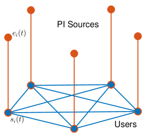
Figure 1: Voter model with personalized information. Graphical representation of the voter model with personalized information. Blue circles represent the agents $s_{i}$ that interact following the usual voter dynamics, while red circles are the external agents, carrying personalized information. Note that the external agent $e_{i}$ influences only the corresponding voter spin, namely $s_{i}$.

To mimic the reinforcing effect of personalized information we assume that, whenever the spin $i$ is selected for update, then $P[e_{i}(t)=+1]$ changes, increasing the probability that $e_{i}$ will be in the future equal to the current state of the agent, $s_{i}$. More precisely at each time step, the update of the probability occurs after the update of the opinion variable. In other words, one first updates the opinion variable (which may or may not change) and afterwards increases by a factor $c$ the ratio between $P[e_{i}=s_{i}(t+\delta t)]$ and $P[e_{i}=-s_{i}(t+\delta t)]$ where $s_{i}(t+\delta t)$ is the opinion variable after the update:

$$\frac{P[e_{i}=s_{i}(t+\delta t)]}{P[e_{i}=-s_{i}(t+\delta t)]}\to c\frac{P[e_{i}=s_{i}(t+\delta t)]}{P[e_{i}=-s_{i}(t+\delta t)]}.$$

In this way the time-depending probability $P(e_{i}=+1)$ keeps track of the history of the spin $s_{i}$. For example if agent $i$ stays in state $s_{i}=+1$ for a long time, then $P(e_{i}=+1)$ tends to grow toward 1 and this makes more likely that opinion $s_{i}=+1$ is maintained. The polarizing effect of this personalized source of information is clear. The parameter $c$ determines the speed at which the balance between the two alternatives is disrupted. Notice that the change for the probability $P(e_{i}=+1)$ occurs at each update of agent $i$, even if the latter does not actually change opinion (because the agent interacts with a neighbor already sharing the same state).

It is useful to define the quantity

$$n_{i}(t)=\sum_{t^{\prime}=1}^{t}s_{i}(t^{\prime}),$$

which keeps memory of the evolution of agent $i$’s opinion. Assuming that initially no knowledge about the agent’s preferences is available and therefore external information is fully random $P[e_{i}(0)=+1]=1/2$ we can write

$$P[e_{i}(t)=1]=P[n_{i}(t)]=\frac{c^{n_{i}(t)}}{1+c^{n_{i}(t)}}.$$ (2)

Hence, a positive (negative) value of $n_{i}$ implies that personalized information is more probably equal to $e_{i}=+1$ ($e_{i}=-1$).

To give a qualitative idea of the model behavior we report in Fig. 2 the temporal evolution of the magnetization $m(t)=\sum_{i}s_{i}/N$ for different values of the probability $\lambda$ of interaction with the personalized information.

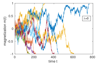
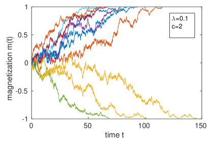
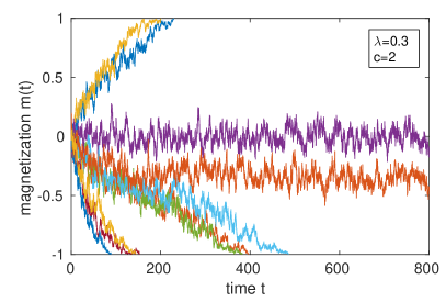
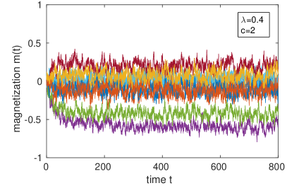
Figure 2: From consensus to polarization. Temporal evolution of the magnetization $m(t)$ for different values of the probability $\lambda$, starting from $\lambda=0$ (pure voter dynamics). Agents form a complete graph of size $N=500$. The trajectories of 10 different runs are displayed.

For $\lambda=0$ the system is exactly the usual voter dynamics and it reaches consensus $m=\pm 1$ because of random diffusive fluctuations, in a time of order $N$ Krapivsky et al. (2010). As personalized information is turned on, consensus is still reached, but surprisingly over shorter time intervals and it is clear that drift plays now a relevant role. Increasing $\lambda$ further we observe that some runs do not reach consensus any more and magnetization fluctuates around some constant value. Finally, for large $\lambda$ consensus is never reached and all runs remain stuck in a disordered state. In the next section, through a mean-field analytical approach, we understand when and how consensus is reached, depending on the values of the parameters $c$ and $\lambda$.

III Analytical results

The evolution of a system following Eqs. (1) and (2) depends on the topology of the network defining the interactions among spins. In the following we will focus on complete graphs, for which each pair of spins is equally likely to interact, meaning that $A_{ij}=1-\delta_{ij}$ for any $(i,j)$. This corresponds, in the absence of external information, to the mean field limit of the voter model. We denote by $N_{\uparrow}$ the number of spins in state $+1$, while $N_{\downarrow}=N-N_{\uparrow}$ is the number of spins in the opposite state. In these terms the updating process is

$$s_{i}(t+\delta t)=\begin{cases}e_{i}(t)\ \text{with probability}\ \lambda\\ +1\ \text{with probability}\ (1-\lambda)\frac{N_{\uparrow}}{N}\\ -1\ \text{with probability}\ (1-\lambda)\frac{N_{\downarrow}}{N},\\ \end{cases}$$ (3)

where the probability of a positive external information is given by Eq. (2). Reminding that the magnetization can be written as

$$m=\frac{N_{\uparrow}-N_{\downarrow}}{N},$$

we obtain from Eq. (3) that each time a node is selected its value $s_{i}$ evolves according to

$$s_{i}(t)\!\to\!s_{i}(t+\delta t)\!=\!\!\begin{cases}\!+1\leavevmode\nobreak\ \leavevmode\nobreak\ \textrm{w. prob:}\leavevmode\nobreak\ (1\!-\!\lambda)\!\left(\frac{1+m}{2}\right)+\lambda P(n_{i})\\ \!-1\leavevmode\nobreak\ \leavevmode\nobreak\ \textrm{w. prob:}\leavevmode\nobreak\ (1\!-\!\lambda)\!\left(\frac{1-m}{2}\right)+\lambda[1\!-\!P(n_{i})].\end{cases}$$ (4)

and, immediately after, $n_{i}$ is updated as follows

$$n_{i}(t)\to n_{i}(t+\delta t)=\begin{cases}n_{i}(t)+1\leavevmode\nobreak\ \leavevmode\nobreak\ \leavevmode\nobreak\ \textrm{if}\leavevmode\nobreak\ \leavevmode\nobreak\ \leavevmode\nobreak\ s_{i}(t+\delta t)=1\\ n_{i}(t)-1\leavevmode\nobreak\ \leavevmode\nobreak\ \leavevmode\nobreak\ \textrm{if}\leavevmode\nobreak\ \leavevmode\nobreak\ \leavevmode\nobreak\ s_{i}(t+\delta t)=-1.\end{cases}$$ (5)

Thus the state of each node is defined by the pair $(s_{i},n_{i})$ and therefore the evolution of the system depends on the set $\left\{(s_{i},n_{i})\right\}_{i=1}^{N}$. In Appendix A we calculate the drift and diffusion coefficients Krapivsky et al. (2010) for the magnetization and for the average value of the $n_{i}$

$$n=\frac{1}{N}\sum_{i}n_{i}.$$ (6)

We obtain the magnetization drift

$$v^{m}=2\frac{\lambda}{N}\sum_{i}\left\{\left(\frac{1-s_{i}}{2}\right)P(n_{i})-\left(\frac{1+s_{i}}{2}\right)[1-P(n_{i})]\right\}$$ (7)

and the magnetization diffusion coefficient

$$D^{m} = \frac{1-\lambda}{N}(1-m^{2})$$

$$+ \frac{2\lambda}{N^{2}}\sum_{i}\left\{\left(\frac{1-s_{i}}{2}\right)P(n_{i})+\left(\frac{1+s_{i}}{2}\right)[1-P(n_{i})]\right\}.$$

For the quantity $n$ the drift coefficient reads

$$v^{n}=(1-\lambda)m+\frac{\lambda}{N}\sum_{i}\left[2P(n_{i})-1\right].$$ (9)

while the diffusion coefficient is

$$D^{n}=\frac{1}{N}.$$ (10)

These expressions contain $P(n_{i})$ and therefore are different depending on the value of $c$.

III.1 The case $c=1$

Let us first discuss the case $c=1$, that is equivalent to the noisy voter model or Kirman model Kirman (1993). In this case Eq. (2) reduces to

$$P(n_{i})=\frac{1}{2}\ \forall\ i,t.$$

and therefore the variables $n_{i}$ do not play any role. Setting $c=1$, Eqs. (7) and (III) reduce to

$$\begin{cases}v^{m}_{c=1}=-\lambda m\\ D^{m}_{c=1}=\frac{1}{N}\left[\left(1-\lambda\right)\left(1-m^{2}\right)+2\lambda\right]\end{cases}$$ (11)

Differently from the standard voter model there is a nonzero drift term, driving the system toward the disordered symmetric configuration $m=0$. However, depending on the value of $\lambda$, the system may still spend most of its time in the consensus state $m=\pm 1$, that is no more absorbing. See Refs. Alfarano et al. (2005); Artime et al. (2018a, b) for a detailed analysis of the noisy voter model.

III.2 The behavior for $c\gtrsim 1$

We now study the behavior for $c>1$, considering separately two cases. We set $c=1+\delta$ and first take $\delta\ll 1$. Under this hypothesis and focusing on short times we can expand $P(n_{i})$ to first order in $n_{i}\delta$, obtaining

$$P(n_{i})=\frac{c^{n_{i}}}{1+c^{n_{i}}}=\frac{(1+\delta)^{n_{i}}}{1+(1+\delta)^{n_{i}}}\approx\frac{1}{2}+\frac{n_{i}\delta}{4}.$$ (12)

Inserting this expression into Eq. (7) we get

$$v^{m}\approx\lambda\left(\frac{n\delta}{2}-m\right),$$ (13)

and analogously for the diffusion coefficient

$$D^{m}\approx\frac{(1-\lambda)}{N}(1-m^{2})+\frac{2\lambda}{N^{2}}\left(1-\frac{\delta}{2N}\sum_{i}s_{i}n_{i}\right).$$ (14)

Inserting the expansion of $P(n_{i})$ into Eq. (9) we obtain

$$v^{n}\approx(1-\lambda)m+\frac{\lambda\delta}{2}n.$$ (15)

In summary, combining Eqs. (13) and (15), the evolution of the system is given, as long as the condition $|n_{i}|\delta\ll 1$ is satisfied for any $i$, by

$$\begin{cases}\dot{m}=-\lambda m+\frac{\lambda\delta}{2}n\\ \dot{n}=(1-\lambda)m+\frac{\lambda\delta}{2}n,\end{cases}$$ (16)

where fluctuations due to diffusion have been neglected. By integrating we find, under the assumption $\delta\ll\lambda$,

$$\begin{cases}m=C_{1}\frac{\delta}{2}\mathrm{e}^{t\delta/2}-C_{2}\frac{\lambda}{1-\lambda}\mathrm{e}^{-\lambda t},\\ n=C_{1}\mathrm{e}^{t\delta/2}+C_{2}\mathrm{e}^{-\lambda t},\end{cases}$$ (17)

where $C_{1}$ and $C_{2}$ are determined by the initial conditions. We note that the deterministic evolution described by Eq. (16) is preceded by a regime dominated by stochastic effects, where we can effectively assume $c=1$. During such an interval $m$ fluctuates around zero due to the presence of the term $-\lambda m$ in its drift, with fluctuations of the order of $\pm m_{0}=\pm\sqrt{D^{m}}\approx\pm\sqrt{(1-\lambda)/N}$. Conversely $n$ grows diffusively, up to the time $\tau=2/\delta$ after which the exponential growth becomes dominant. Moreover, after a short time of order $1/\lambda$ the terms proportional to $C_{2}$ in Eqs. (17) become negligible. As a consequence we can use as initial condition for $n$ its value at time $\tau$, i.e., at the end of the diffusive regime, yielding $C_{1}\approx\sqrt{\tau D_{n}}\approx\sqrt{\frac{2}{\delta N}}$

$$\begin{cases}n\approx\pm\sqrt{\frac{2}{\delta N}}\mathrm{e}^{t\delta/2}\\ m=\frac{\delta}{2}n.\end{cases}\text{for}\ t>\tau$$ (18)

Note that the exponential growth of $m$ actually begins only when $\frac{\delta}{2}|n|\sim m_{0}\approx\sqrt{(1-\lambda)/N}$. Fig. 3 shows that Eq. (18) describes well this stage of the temporal evolution of $n$ and $m$.

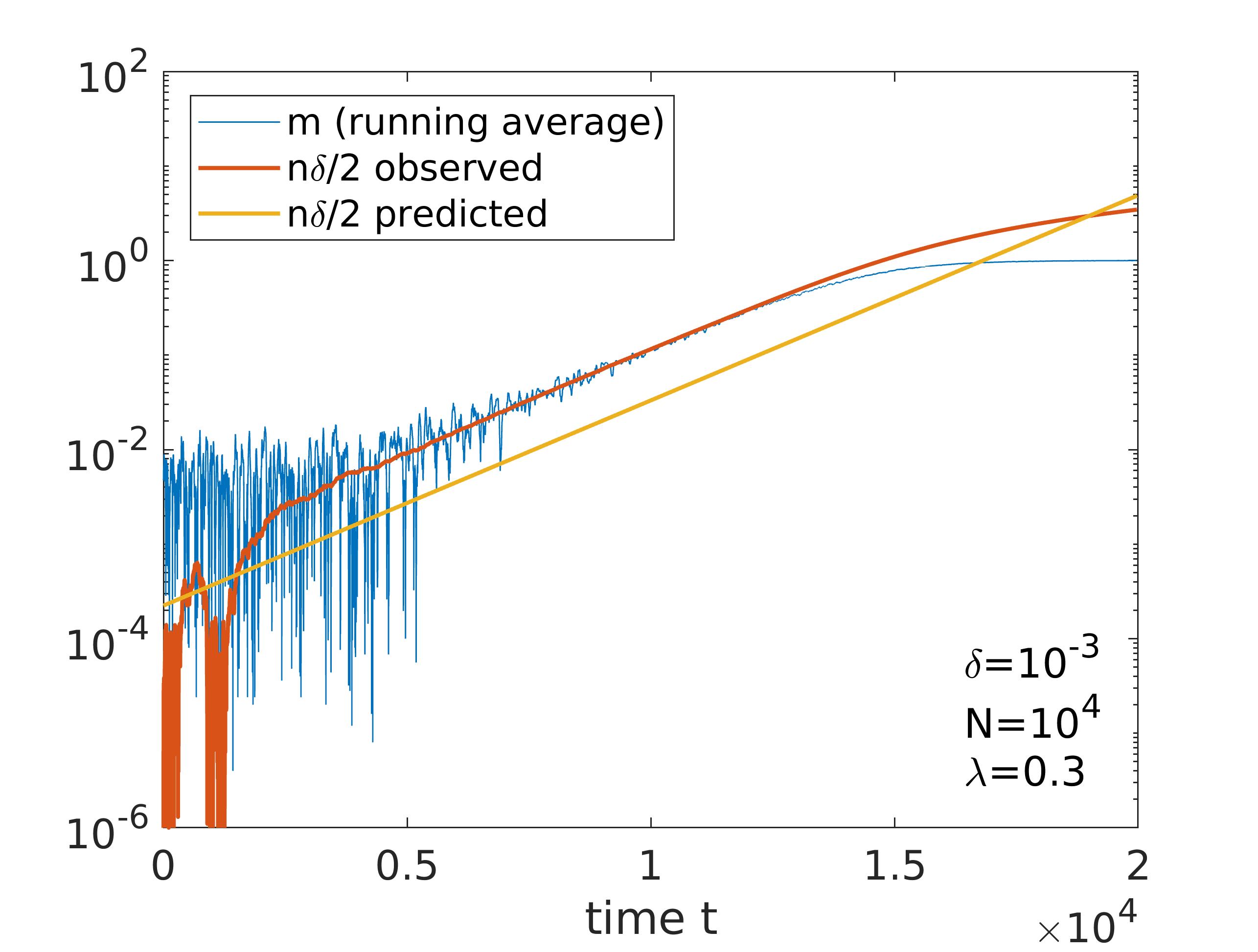
Figure 3: Growth of $n$ and $m$. Growth of $m$ compared with the observed $n\delta/2$ and with the predicted trend, as defined by Eq. (18). $n$ grows diffusively up to $\tau=2/\delta$, time at which the exponential contribution becomes dominant.

The linear approximation remains valid until the time $T_{c}$ when, for some $i$, $|n_{i}|$ becomes so large that the condition $|n_{i}|\delta\ll 1$ breaks down. This may happen in two different ways, depending on the shape of the probability distribution $Q(n_{i})$ of the variables $n_{i}$. When the linear approximation breaks down, if the standard deviation of $Q(n_{i})$ is small, the personalized information is approximately the same for all individuals. As a consequence this source of information can be regarded as a constant field and this results in the presence of a drift for the magnetization, which fastly reaches $m=\pm 1$. Conversely, if the standard deviation is much larger than the average $\langle n_{i}\rangle$, some of the spins are characterized by a negative $n_{i}$, while $n_{i}$ is positive for the others. This implies that a fraction of the spins is influenced by a positive external field, while a negative field acts on the remaining part, thus leading to a polarized state. More in detail, if $Q(n_{i})$ is narrowly peaked around its mean value $n$ over time, linearization breaks down for a time $T$ such that $|n(T)|\delta\sim 1$. From Eq. (18)

$$T=\frac{1}{\delta}\log\left(\frac{N}{2\delta}\right).$$ (19)

At this time all $n_{i}$ have the same sign, hence the drift (see Appendix A)

$$v_{i}=m(T)(1-\lambda)+\lambda[2P(n_{i})-1],$$ (20)

has the same sign for all individuals and thus consensus is rapidly reached.

Alternatively, if the distribution is very broad so that its standard deviation $\sigma$ is much larger than the absolute mean value $|n|$, linearization starts to fail at a different time $T^{*}$. Assuming, for the sake of simplicity, $n>0$, this occurs when

$$\delta[n+\sigma(T^{*})]\approx\delta\sigma(T^{*})=1$$ (21)

The calculation of the variance $\sigma^{2}(t)$ of the distribution $Q(n_{i})$, reported in Appendix B, gives

$$\sigma^{2}(t)=\frac{1}{\lambda\delta}\left(\mathrm{e}^{\lambda\delta t}-1\right).$$ (22)

Imposing $\delta\sigma(T^{*})=1$ we then obtain

$$T^{*}=\frac{1}{\lambda\delta}\log\left(1+\frac{\lambda}{\delta}\right).$$ (23)

The time $T_{c}$ when the linear approximation breaks down consequently is

$$T_{c}=\min(T,T^{*}).$$

Since $T$ grows with $N$, while $T^{*}$ does not depend on it, for small size $T<T^{*}$ and the opposite relationship $T>T^{*}$ is instead true for large $N$. Setting $T=T^{*}$ we can compute the crossover size

$$N^{*}=2\delta\left(1+\frac{\lambda}{\delta}\right)^{1/\lambda}.$$ (24)

For $N<N^{*}$ linearization breaks down due to the growth of $n$ and as a consequence consensus is always reached, all the drifts having the same sign. Differently, if $N>N^{*}$ the end of the linear regime is caused by the growth of the variance. In this second case, at $T^{*}$ most of the individuals have positive $n_{i}$ and hence a positive drift, but some have negative $n_{i}$ (see Fig. 4). Determining in this case whether consensus is reached or not is more involved, as discussed in the following.

Assuming $N\gg N^{*}$, so that the standard deviation is much larger than the mean value, the smallest of the negative values is

$$n_{i}\approx n-\sigma(T^{*})\approx-\sigma(T^{*})\approx-\frac{1}{\delta},$$ (25)

and as a consequence the smallest drift is

$$v_{i}=m(T^{*})(1-\lambda)+\lambda[2P(n_{i})-1]\approx m(T^{*})(1-\lambda)-\lambda.$$ (26)

If this value is positive, the corresponding individual, which is the one whose external information is more negatively polarized, will be pushed towards positive values of $n_{i}$. It then follows that also in this case the system reaches consensus.

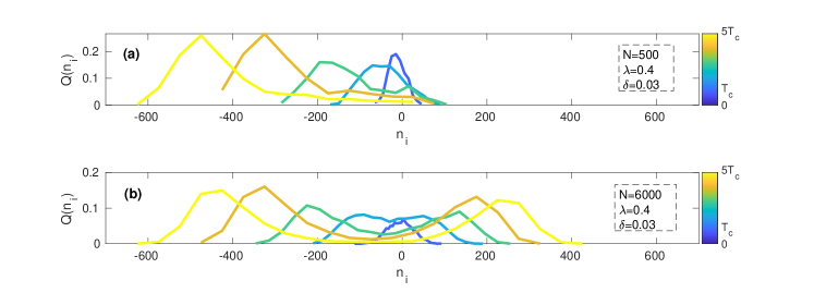
Figure 4: Evolution of $Q(n_{i})$. Evolution of $Q(n_{i})$ for $N<N_{c}$ (panel (a)) and $N>N_{c}$ (panel (b)).

More quantitatively, the condition for having consensus, $v_{i}>0$, implies (considering also the symmetric case when $n<0$)

$$|m(T^{*})|>\frac{\lambda}{1-\lambda}=m_{c}.$$ (27)

Inserting Eq. (23) into Eq. (18) we obtain

$$|m(T^{*})|=\sqrt{\frac{\delta}{2N}}\left(1+\frac{\lambda}{\delta}\right)^{\frac{1}{2\lambda}},$$ (28)

that combined with the condition (27) implies that consensus is undoubtedly reached for $\lambda<1/2$ if $N<\bar{N}$, with

$$\bar{N}=\frac{(1-\lambda)^{2}}{\lambda^{2}}\frac{\delta}{2}\left(1+\frac{\lambda}{\delta}\right)^{\frac{1}{\lambda}}.$$ (29)

Note, however, that this is only a lower bound for the true $N_{c}$ for $\lambda<1/2$. Actually consensus may occur also for $N>\bar{N}$, provided that $\lambda<1/2$. Indeed, even if the smallest drift (corresponding to the most negative $n_{i}$) is negative when linearization breaks down, it can become positive later on, thus making the system reach consensus. This may occur if only a few spins (among those with $n_{i}<0$) have a negative drift. The others, moving toward positive $n_{i}$, produce an increase of the magnetization, which eventually overcomes the critical value $m_{c}=\frac{\lambda}{1-\lambda}$. The critical size $N_{c}$, determining if the system can reach consensus or not, is then larger than $\bar{N}$ for $\lambda<1/2$. It is actually possible to improve on this result. In Appendix C a more refined argument is presented, allowing us to determine numerically a tighter lower bound $\hat{N}$ for $N_{c}$. This bound, as shown in Fig. 5, is in good agreement with simulations.

The situation is different if $\lambda\geq 1/2$, because in this case the critical magnetization is larger than 1 and therefore, even if some spins move from negative $n_{i}$ to positive $n_{i}$, the smallest drift remains negative, for any magnetization. This implies that for $\lambda\geq 1/2$, consensus can be reached only if linearization breaks down due to the growth of $n$. Therefore if $\lambda\geq 1/2$, the critical size coincides with $N^{*}$. In conclusion

$$\begin{cases}N_{c}\geq\hat{N}\leavevmode\nobreak\ \leavevmode\nobreak\ \leavevmode\nobreak\ \leavevmode\nobreak\ \leavevmode\nobreak\ \leavevmode\nobreak\ \leavevmode\nobreak\ \leavevmode\nobreak\ \leavevmode\nobreak\ \leavevmode\nobreak\ \leavevmode\nobreak\ \leavevmode\nobreak\ \leavevmode\nobreak\ \leavevmode\nobreak\ \leavevmode\nobreak\ \leavevmode\nobreak\ \leavevmode\nobreak\ \leavevmode\nobreak\ \leavevmode\nobreak\ \leavevmode\nobreak\ \leavevmode\nobreak\ \leavevmode\nobreak\ \leavevmode\nobreak\ \leavevmode\nobreak\ \text{for}\ \lambda<\frac{1}{2}\\ N_{c}=N^{*}=2\delta\left(1+\frac{\lambda}{\delta}\right)^{1/\lambda}\ \text{for}\ \lambda\geq\frac{1}{2}.\end{cases}$$ (30)

Of course, given the dependence of the argument on random fluctuations, these values are to be intended as indicating a crossover and not a sharp transition. Simulation results presented in Fig. 5 confirm that the probability of reaching consensus exhibits for various $\lambda$, a crossover in reasonable agreement with Eq. (30).

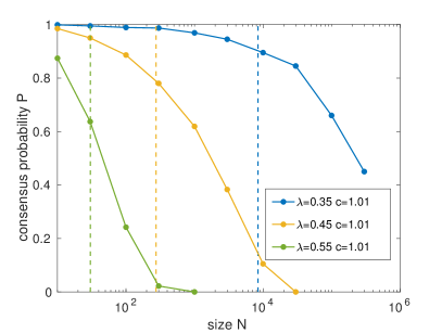
Figure 5: Crossover between consensus and polarization for small $c$. Fraction of runs reaching consensus as a function of $N$, in 1000 realizations of the dynamics for $\delta=0.01$ and various $\lambda$. The crossover values $N_{c}$ predicted by Eq. (30) are marked by vertical lines.

III.3 The behavior for $c\gg 1$

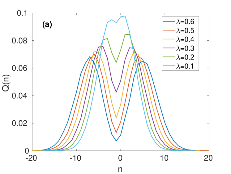
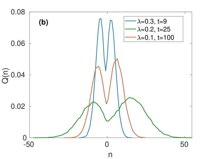
Figure 6: Splitting of $Q(n_{i})$. a) Distribution $Q(n_{i})$ at $t=10$ for various values of $\lambda$. Note that, for $\lambda=0.1$, $t\ll t_{c}=100$ while for $\lambda=0.6$ $t\gg t_{c}=2.77$. b) Distribution $Q(n_{i})$ at $t\approx t_{c}=1/\lambda^{2}$ for various values of $\lambda$.

As shown in the previous subsection, if $c$ is close to $1$ the system can be described in terms of the magnetization and of the first two moments of the distribution $Q(n_{i})$, $n$ and $\sigma^{2}$. This is possible because (see Fig. 4) this distribution is unimodal during the linear regime, that lasts for long times, up to $T_{c}=\min(T,T^{*})$. Conversely, when $c$ is large, the pair $(n,\sigma^{2})$ alone is not sufficient to describe the state of the system, even in the first stage of the dynamics. This can be seen by inspecting the local probabilities $P(n_{i})$. If $c\gg 1$ we have

$$P(n_{i})=\begin{cases}1-c^{-n_{i}}\approx 1\ \leavevmode\nobreak\ \leavevmode\nobreak\ \text{if}\ n_{i}>0\\ \frac{1}{2}\ \leavevmode\nobreak\ \leavevmode\nobreak\ \leavevmode\nobreak\ \leavevmode\nobreak\ \leavevmode\nobreak\ \leavevmode\nobreak\ \leavevmode\nobreak\ \leavevmode\nobreak\ \leavevmode\nobreak\ \leavevmode\nobreak\ \leavevmode\nobreak\ \leavevmode\nobreak\ \leavevmode\nobreak\ \leavevmode\nobreak\ \leavevmode\nobreak\ \leavevmode\nobreak\ \text{if}\ n_{i}=0\\ c^{n}\approx 0\ \leavevmode\nobreak\ \leavevmode\nobreak\ \leavevmode\nobreak\ \leavevmode\nobreak\ \leavevmode\nobreak\ \leavevmode\nobreak\ \leavevmode\nobreak\ \leavevmode\nobreak\ \leavevmode\nobreak\ \leavevmode\nobreak\ \text{if}\ n_{i}<0.\end{cases}$$

This means that, as soon as $n_{i}$ becomes different from zero at the first update of node $i$, the external information almost certainly has the same sign of $n_{i}$ and thus tends to increase its absolute value. The behavior of nodes with different signs of $n_{i}$ is opposite and this rapidly leads to the splitting of $Q(n_{i})$ in two separate peaks. We then write the overall distribution as the sum of two unimodal distributions

$$Q(n_{i})=pQ^{+}(n_{i})+(1-p)Q^{-}(n_{i}).$$

Here $Q^{+}(n_{i})$ is the distribution of positive $n_{i}$, while $Q^{-}(n_{i})$ is the distribution of the negative ones and the weight is $p=N^{+}/N$. By using the same formalism described above, in Appendix D we derive expressions for the moments of the two distributions

$$v^{\pm}=\frac{d\langle n_{i}\rangle_{\pm}}{dt}=m(1-\lambda)\pm\lambda,$$ (31)

$$\sigma^{2}_{\pm}=t.$$ (32)

Since $m$ is initially very small, Eq. (31) confirms that positive (negative) $n_{i}$ tend to increase (decrease) and the overall distribution $Q(n_{i})$ broadens and eventually splits. In the same Appendix we derive the expression for the variance $\sigma^{2}(t)=\langle n_{i}^{2}\rangle-\langle n_{i}\rangle^{2}$ of the whole distribution $Q(n_{i})$, finding

$$\sigma^{2}(t)=t+\lambda^{2}t^{2}.$$ (33)

From Eq. (33) we can determine the time at which $Q(n_{i})$ splits in two separate components. For small times $\sigma(t)$ is dominated by the diffusive widening of the central peak, while for larger times it is determined mainly by the ballistic distancing between the two peaks. Denoting by $t_{c}$ the time at which the crossover occurs, it follows from Eq. (33) $t_{c}\approx\lambda^{2}t_{c}^{2}$ yielding

$$t_{c}\approx\frac{1}{\lambda^{2}}.$$

Figures 6a and 6b confirm numerically this prediction. Note that, at odds with the case $c\gtrsim 1$, the splitting always occurs, and over a much shorter temporal scale since $t_{c}=1/\lambda^{2}\ll\log(1+\lambda/\delta)/(\lambda\delta)=T^{*}$.

To understand whether the system reaches consensus or not, the argument is similar to the one presented for $c\gtrsim 1$, but in this case it provides the actual critical size $N_{c}$ rather than a lower bound. If, when the distribution splits, the drift of the right peak is positive and that of the left peak is negative, consensus is not reached. From Eq. (31) this implies that consensus is reached only if

$$|m(t_{c})|>m_{c}=\frac{\lambda}{1-\lambda}.$$ (34)

This condition means, as before, that consensus for $\lambda>1/2$ can occur only before the splitting, so during the transient regime. It turns out numerically that, for $t<t_{c}$, the magnetization $m$ grows as $m(t)\approx\xi t/\sqrt{N}$, where $\xi$ is a random prefactor ranging between approximately -1 and +1. Hence for $\lambda>1/2$ the condition for consensus reads

$$|m(t)|=1\ \text{for}\ t<t_{c}\ \to\ \frac{t_{c}}{\sqrt{N_{c}}}=1\ \to\ N_{c}=\frac{1}{\lambda^{4}}.$$

For $\lambda<1/2$ instead, inserting the expression for $m(t)$ into Eq. (34) yields that consensus cannot be reached if the number $N$ of individuals is larger than

$$N_{c}=\frac{(1-\lambda)^{2}}{\lambda^{6}}.$$ (35)

For $N>N_{c}$ the system remains asymptotically disordered in a polarized state. In the opposite case instead consensus is rapidly reached after $t_{c}$, unless by chance the initial absolute value of $\xi$ is particularly small.

In conclusion, recalling Eq. (35), the critical size satisfies

$$\begin{cases}N_{c}=\frac{(1-\lambda)^{2}}{\lambda^{6}}\leavevmode\nobreak\ \leavevmode\nobreak\ \leavevmode\nobreak\ \text{for}\ \lambda<\frac{1}{2}\\ N_{c}=\frac{1}{\lambda^{4}}\leavevmode\nobreak\ \leavevmode\nobreak\ \leavevmode\nobreak\ \leavevmode\nobreak\ \leavevmode\nobreak\ \leavevmode\nobreak\ \leavevmode\nobreak\ \leavevmode\nobreak\ \text{for}\ \lambda\geq\frac{1}{2}.\end{cases}$$ (36)

Note that $N_{c}$ is continuous in $\lambda=1/2$. Simulations presented in Fig. 7 show that the probability of reaching consensus exhibits a crossover at values well predicted by Eq. (36).

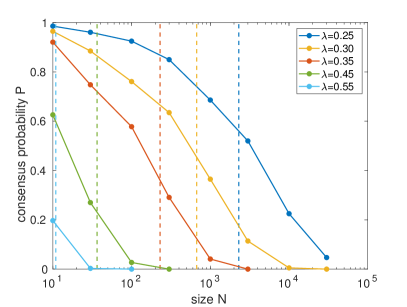
Figure 7: Crossover between consensus and polarization for large $c$. Fraction of runs reaching consensus as a function of $N$, in 1000 realizations of the dynamics for $c=100$ and several $\lambda$ values. The crossover values $N_{c}$ predicted by Eq. (36) are marked by vertical lines.

The long time dynamics in the case $c\gg 1$ can be studied also in more detail, by describing the evolution of the two peaks and their mutual interaction. As shown in Appendix E we can write a closed integro-differential equation for the magnetization $m(t)$. In particular, defining

$$y=\int_{0}^{t}m(t^{\prime})dt^{\prime}$$

we obtain the following second order non linear ODE:

$$\frac{d^{2}y}{dt^{2}}=\sqrt{\frac{2}{\pi t(1-\lambda)^{2}}}\left\{\left(1-\frac{dy}{dt}\right)\frac{1}{\frac{1}{t}y-m_{c}}\exp\left[-\frac{t(1-\lambda)^{2}\left(\frac{1}{t}y-m_{c}\right)^{2}}{2}\right]-\left(1+\frac{dy}{dt}\right)\frac{1}{\frac{1}{t}y+m_{c}}\exp\left[-\frac{t(1-\lambda)^{2}\left(\frac{1}{t}y+m_{c}\right)^{2}}{2}\right]\right\}.$$ (37)

Note that the evolution of $m(t)$ is expressed in terms of $y$, which is a variable containing the past history of the system. This reflects the fact that personalized information keeps memory of the preferences of the spin it is coupled to. The fact that the evolution of $m$ is governed by an integro-differential equation is then a very natural consequence of the dynamics of the model. Solutions of this equation are reported in Fig. 8b, where it is possible to see that states with $|m|<m_{c}$ remain disordered, while if $m<-m_{c}$ or $m>m_{c}$ consensus is reached, in good agreement with numerical simulations, shown in Fig. 8a.

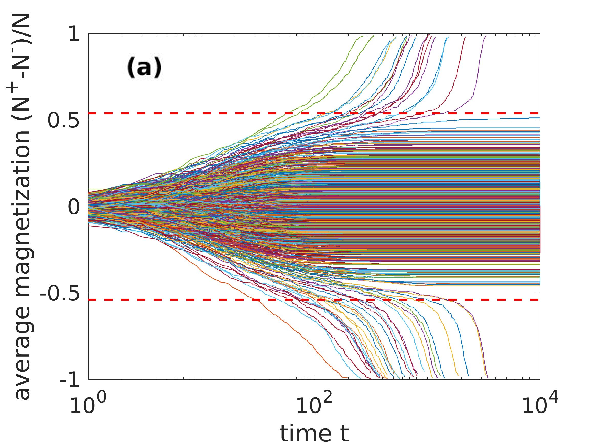
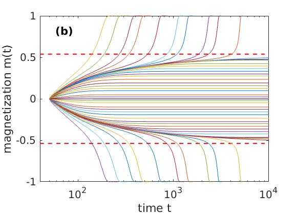
Figure 8: Time evolution of the magnetization for $c=100$. (a) $10^{4}$ trajectories obtained simulating the model with $N=10^{3}$, $c=100$ and $\lambda=0.35$. Red dashed lines represent $\pm m_{c}=\pm\lambda/(1-\lambda)$, disordered states are found in the region $[-m_{c};+m_{c}]$. (b) Solutions of Eq. (37) for $\lambda=0.35$ and various $m_{0}$ in the range $10^{-5};10^{-3}$. The differential equation is valid only for times much larger than $t_{c}\approx 8$, therefore we set $t_{0}=50$. As initial condition for the variable $y_{0}$ we used $y_{0}=y(t_{0})=m_{0}t^{2}/2$, because the magnetization grows linearly during the initial regime. Red dashed lines represent $\pm m_{c}=\pm\lambda/(1-\lambda)$, also in this case disordered states are found in the region $[-m_{c};+m_{c}]$.

Disordered states for $c>1$ are completely different from the disordered states for $c=1$. In the latter case the constant magnetization is the effect of the external information being a random uncorrelated variable equal for all nodes so that all agents spend half of their time with $s_{i}=+1$ and half with $s_{i}=-1$. For $c>1$ instead, the system is divided in two polarized clusters whose agents have a preferred spin value. A further characterization in terms of self-overlap is presented in Appendix F.

IV Discussion and conclusions

Let us summarize the results of our investigation. The evolution of the system is described by the magnetization $m$ and the distribution of the local quantities $n_{i}$, describing the personalized information for each agent. Depending on whether $\delta$ ($c=1+\delta$) is much smaller or much larger than $1$ the temporal evolution exhibits some variation.

In the first case there are three temporal regimes in the evolution of the system. For short times up to $2/\delta$ stochastic effects dominate, the magnetization fluctuates around zero and the distribution of the local $n_{i}$ remains centered around zero. Later on the symmetry between positive and negative external information breaks down because the mean value $n(t)$ of the single-peaked distribution $Q(n_{i})$ starts drifting away from $n=0$ exponentially in time, while also its width $\sigma(t)$ grows. At the same time also $|m|$ grows exponentially. This regime ends when linearization of the equations for $m$ and $n$ is no more valid. The nonlinear subsequent evolution varies depending on the relative width of the peak. If the peak is narrow, all $n_{i}$ have the same sign and consensus is quickly reached. If the peak is broad then individuals with both $n_{i}>0$ and $n_{i}<0$ exist. If the magnetization in this moment is small enough then the system gets trapped in a disordered (polarized) state, where disagreement persists and the magnetization keeps a constant value $|m|<m_{c}=\lambda/(1-\lambda)$.

When $\delta\gg 1$ (i.e., $c\gg 1$) linearization is never valid, the $Q(n_{i})$ distribution always splits in two components and this happens much earlier, over a time scale equal to $t_{c}=1/\lambda^{2}$. What happens next depends again on the value of the magnetization at $t_{c}$. If $|m(t_{c})|$ is sufficiently large, the drift of the two components has the same sign. For example, if this sign is positive, it means that individuals with negative $n_{i}$ have nevertheless an overall positive drift: The negative component of the $Q(n_{i})$ distribution gets rapidly depleted and consensus is reached. Otherwise the competition between the two opinions persists forever and the system gets stuck in the polarized state with $m<m_{c}$.

Although the detailed temporal evolution is rather different depending on whether $c=1+\delta$ is very close to 1 or much larger, the final overall phenomenology is similar. The parameter $c$ sets the temporal scales of the dynamics and the details of the phase-diagram, but not the qualitative features of the behavior: consensus for $N<N_{c}(\lambda)$, polarization otherwise. The dependence of $N_{c}$ on $\lambda$ is different depending on whether $c$ is close to 1 [Eq. (30)] or large [Eq. (36)], so the boundaries between the two regions depend on the value of $c$. Fig. 9 represents this phase-diagram for several of these values, showing that, as expected, increasing the strength of personalized information makes consensus more difficult.

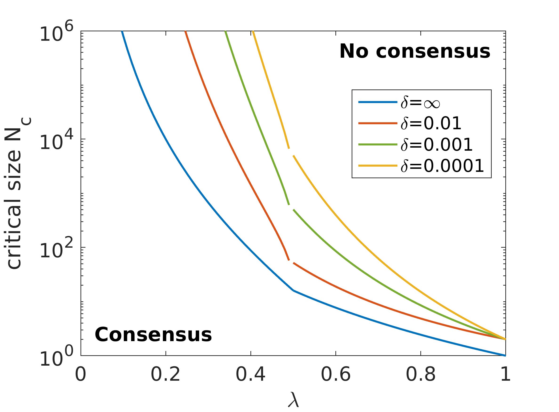
Figure 9: Phase-diagram for all $c$. The lines separate the region where consensus is reached from the region where it is not. Lines are obtained using Eq. (30) for $\delta\ll 1$ and Eq. (36) for $\delta=\infty$.

However, we observe that increasing $c$ reduces the consensus region but with a nontrivial limit: even in the $c\to\infty$ limit, consensus is possible in sufficiently small systems.

This rather rich phenomenology has been obtained in the simplest possible setting: an extremely simple binary opinion dynamics always leading to consensus, in a mean-field framework, augmented with an elementary form of personalized information. Clearly our results open some interesting issues for future research: What is the effect of a less trivial contact pattern among agents? What changes when different opinion dynamics models are considered? What happens if personalized information is parameterized differently, for example considering different functional forms for the probability $P(n_{i})$? Finally, despite our oversimplified assumptions, some predictions derived in this work may be testable in empirical systems. In particular, the fact that disordered states cannot have magnetization larger than $m_{c}$ or the existence of a maximum size $N_{c}$ for the reaching of consensus could be observable in systems where a community has to decide between two alternative options.

Appendix A Drift and diffusion coefficients

Let us define as $R_{i}$ the probability that $s_{i}$ switches from $-1$ to $+1$ in a single update. Eq. (4) implies

$$R_{i}=\frac{1}{N}\left[\frac{1-\lambda}{N}\left(\frac{1-s_{i}}{2}\right)\underbrace{\sum_{j}\left(\frac{1+s_{j}}{2}\right)}_{N_{\uparrow}}+\lambda\left(\frac{1-s_{i}}{2}\right)P(n_{i})\right],$$

where the prefactor stems from the fact that the $i$th spin is selected with probability $1/N$. Analogously $L_{i}$ is the probability of the opposite transition, namely from $s_{i}=+1$ to $s_{i}=-1$:

$$L_{i}=\frac{1-\lambda}{N^{2}}\left(\frac{1+s_{i}}{2}\right)\underbrace{\sum_{j}\left(\frac{1-s_{j}}{2}\right)}_{N_{\downarrow}}+\frac{\lambda}{N}\left(\frac{1+s_{i}}{2}\right)\left[1-P(n_{i})\right].$$

We can obtain the corresponding transition probabilities for the magnetization $m$ by summing over all spins

$$R^{m} = (1-\lambda)\frac{1-m}{2}\cdot\frac{1+m}{2}+\frac{\lambda}{N}\sum_{i}\left(\frac{1-s_{i}}{2}\right)P(n_{i}),$$

$$L^{m} = (1-\lambda)\frac{1+m}{2}\cdot\frac{1-m}{2}+\frac{\lambda}{N}\sum_{i}\left(\frac{1+s_{i}}{2}\right)\left[1-P(n_{i})\right].$$

In a single update, occurring in a time $\delta t=1/N$, the variation of the magnetization is $\delta m=2/N$, hence its drift is

$$v^{m} = \frac{\delta m}{\delta t}[R^{m}-L^{m}]$$

$$= 2\frac{\lambda}{N}\sum_{i}\left\{\left(\frac{1-s_{i}}{2}\right)P(n_{i})-\left(\frac{1+s_{i}}{2}\right)[1-P(n_{i})]\right\}$$

Analogously the diffusion coefficient is

$$D^{m} = \frac{(\delta m)^{2}}{\delta t}[R^{m}+L^{m}]=\frac{1-\lambda}{N}(1-m^{2})$$

$$+ \frac{2\lambda}{N^{2}}\sum_{i}\left\{\left(\frac{1-s_{i}}{2}\right)P(n_{i})+\left(\frac{1+s_{i}}{2}\right)[1-P(n_{i})]\right\}$$

As expected, the evolution of the magnetization depends also on the variables $n_{i}$, encoding the probability of the personalized information. For this reason it is necessary to consider in detail their evolution. Their transition probabilities are

$$R^{n_{i}}=\frac{1}{N}\left[(1-\lambda)\left(\frac{1+m}{2}\right)+\lambda P(n_{i})\right],$$ (38)

$$L^{n_{i}}=\frac{1}{N}\left[(1-\lambda)\left(\frac{1-m}{2}\right)+\lambda[1-P(n_{i})]\right].$$

The difference between these probabilities and those for the $s_{i}$ stems from the fact that $n_{i}$ is updated at each step, not only when $s_{i}$ changes its state. Using these expressions we can determine the drift for individual variables $n_{i}$

$$v_{i}=\frac{\delta n_{i}}{\delta t}(R^{n_{i}}-L^{n_{i}})=(1-\lambda)m+\lambda[2P(n_{i})-1].$$ (39)

Summing the transition probabilities over all nodes we obtain the probabilities for $n$:

$$R^{n}=\sum_{i}R^{n_{i}}=(1-\lambda)\left(\frac{1+m}{2}\right)+\frac{\lambda}{N}\sum_{i}P(n_{i}),$$

$$L^{n}=\sum_{i}L^{n_{i}}=(1-\lambda)\left(\frac{1-m}{2}\right)+\frac{\lambda}{N}\sum_{i}[1-P(n_{i})].$$

In this case the variation in a single update is $\delta n=1/N$, as a consequence the drift coefficient reads

$$v^{n}=\frac{\delta n}{\delta t}[R^{n}-L^{n}]=(1-\lambda)m+\frac{\lambda}{N}\sum_{i}\left[2P(n_{i})-1\right].$$ (40)

The diffusion coefficient is instead

$$D^{n}=\frac{(\delta n)^{2}}{\delta t}[R^{n}+L^{n}]=\frac{1}{N}\left[(1-\lambda)+\frac{\lambda}{N}\sum_{i}1\right]=\frac{1}{N}.$$ (41)

Appendix B Variance of $Q(n_{i})$ for $c\gtrsim 1$

The master equation governing the evolution of $Q(n_{i})$ is

$$Q(n_{i},t+\delta t)= R^{n_{i}-1}Q(n_{i}-1,t)+L^{n_{i}+1}Q(n_{i}+1,t)+$$

$$+\left(1-R^{n}-L^{n}\right)Q(n_{i},t),$$

where $1-R^{n}-L^{n}=(1-1/N)$ is the probability that the spin $i$ is not selected and thus not updated. Expanding for small $\delta t$ we obtain

$$\frac{d}{dt}Q(n_{i})=\frac{1}{\delta t}[ R^{n_{i}-1}Q(n_{i}-1,t)+L^{n_{i}+1}Q(n_{i}+1)$$

$$-\left(R^{n}+L^{n}\right)Q(n_{i})],$$ (42)

where $\delta t=1/N$ and the transition probabilities $R^{n_{i}}$ are given by Eq. (38). Noticing that $R^{n}+L^{n}=\frac{1}{N}$ we rewrite this equation as

$$\frac{d}{dt}Q(n_{i})= NR^{n_{i}-1}Q(n_{i}-1,t)+\left(1-NR^{n_{i}+1}\right)Q(n_{i}+1)$$

$$-Q(n_{i}),$$ (43)

Using the condition $|n_{i}|\delta\ll 1$ we rewrite the transition probabilities as

$$R^{n_{i}}=\frac{1}{N}\left[(1-\lambda)\left(\frac{1+m}{2}\right)+\lambda\left(\frac{1}{2}+\frac{1}{4}\delta n_{i}\right)\right].$$ (44)

Substituting this expression into Eq. (43), multiplying by $n_{i}^{2}$ and summing over $n_{i}$ we obtain

$$\frac{d}{dt}\langle n_{i}^{2}\rangle = \sum_{n_{i}}\left[4NR^{n_{i}}n_{i}Q(n_{i})+(1-2n_{i})Q(n_{i})\right]$$ (45)

$$= 2m(1-\lambda)\langle n_{i}\rangle+1+\lambda\delta\langle n_{i}^{2}\rangle,$$

where $\langle n_{i}\rangle$ is the quantity $n$ defined in Eq. (6). The variance of $Q(n_{i})$ is $\sigma^{2}=\langle n_{i}^{2}\rangle-\langle n_{i}\rangle^{2}$, hence using Eqs. (16) and (45) we get

$$\frac{d}{dt}\sigma^{2}= \frac{d}{dt}\langle n_{i}^{2}\rangle-2\langle n_{i}\rangle\frac{d}{dt}\langle n_{i}\rangle$$

$$= 2m(1-\lambda)\langle n_{i}\rangle+1+\lambda\delta\langle n_{i}^{2}\rangle$$

$$-2\langle n_{i}\rangle\left[(1-\lambda)m+\frac{\delta\lambda}{2}\langle n_{i}\rangle\right]$$

$$= 1+\lambda\delta\sigma^{2},$$

whose solution, with initial condition $\sigma^{2}(0)=0$, is

$$\sigma^{2}(t)=\frac{1}{\lambda\delta}\left(\mathrm{e}^{\lambda\delta t}-1\right).$$ (46)

Appendix C A more refined lower bound for $N_{c}$

The drift of spin $i$ is given by Eq. (26)

$$v_{i}=m(1-\lambda)+\lambda\left[2P(n_{i})-1\right].$$

For small $\delta=c-1$, the probability $P(n_{i})$ can be expanded, giving

$$P(n_{i})=\frac{1}{2}+\frac{n_{i}\delta}{4},$$

therefore

$$v_{i}=m(1-\lambda)+\lambda\frac{n_{i}\delta}{2}.$$

As a consequence the spins with negative drift are those whose $n_{i}$ satisfies $n_{i}<\bar{n}$, with $\bar{n}$ defined by

$$m(1-\lambda)+\lambda\frac{\bar{n}\delta}{2}=0\ \to\ \bar{n}=-\frac{2m}{\delta}\frac{1-\lambda}{\lambda}=-\frac{2}{\delta}\frac{m}{m_{c}}.$$ (47)

We assume that at time $T^{*}$, when linearization breaks down, all spins with $n_{i}<0$, but positive drift $v_{i}(T^{*})>0$, will eventually end up with $n_{i}\to+\infty$, while those with $v_{i}(T^{*})<0$ will drift toward $-\infty$. The number of spins with $v_{i}(T^{*})<0$ is easily obtained by integrating the distribution $Q_{t}(n_{i})$ and using Eq. (47). More precisely, denoting this quantity by $N^{-}_{\infty}$, it holds

$$N^{-}_{\infty}=N\int_{-\infty}^{\bar{n}}Q(n_{i})dn_{i}=N\int_{-\infty}^{-\frac{2}{\delta}\frac{m(T^{*})}{m_{c}}}Q_{T^{*}}(n_{i})dn_{i}.$$

The distribution $Q_{t}(n_{i})$ can be approximated by a Gaussian with mean value $n(t)$ and variance $\sigma^{2}(t)$. At time $T^{*}$ the variance satisfies by definition

$$\sigma^{2}(T^{*})=\frac{1}{\delta^{2}},$$

while recalling that

$$n(t)=\sqrt{\frac{2}{\delta N}}\mathrm{e}^{t\delta/2},\quad T^{*}=\frac{1}{\lambda\delta}\log\left(1+\frac{\lambda}{\delta}\right),$$

we get

$$n(T^{*})=\sqrt{\frac{2}{\delta N}}\left(1+\frac{\lambda}{\delta}\right)^{\frac{1}{2\lambda}}.$$ (48)

Asymptotically, the number of negative spin can then be written as

$$N^{-}_{\infty}=\frac{N}{\sqrt{2\pi\sigma^{2}(T^{*})}}\int_{-\infty}^{-\frac{2}{\delta}\frac{m(T^{*})}{m_{c}}}\exp\left[-\frac{\left(n(T^{*})-n_{i}\right)^{2}}{2\sigma^{2}(T^{*})}\right]dn_{i}=$$

$$=\frac{N\delta}{\sqrt{2\pi}}\int_{-\infty}^{-\frac{2}{\delta}\frac{m(T^{*})}{m_{c}}}\exp\left\{-\frac{\left[\sqrt{\frac{2}{\delta N}}\left(1+\frac{\lambda}{\delta}\right)^{\frac{1}{2\lambda}}-n_{i}\right]^{2}\delta^{2}}{2}\right\}dn_{i}$$

The asymptotic magnetization $m_{\infty}$ will consequently be

$$m_{\infty}=\frac{N^{+}_{\infty}-N^{-}_{\infty}}{N}=\frac{N-2N^{-}_{\infty}}{N}=$$

$$=1-2\frac{\delta}{\sqrt{2\pi}}\int_{-\infty}^{-\frac{2}{\delta}\frac{m(T^{*})}{m_{c}}}\exp\left\{-\frac{\left[\sqrt{\frac{2}{\delta N}}\left(1+\frac{\lambda}{\delta}\right)^{\frac{1}{2\lambda}}-n_{i}\right]^{2}\delta^{2}}{2}\right\}dn_{i}.$$

The asymptotic state is disordered only if this magnetization is smaller than the critical magnetization, otherwise the drift of the negative peak is positive and therefore consensus is reached. The condition for consensus consequently reads

$$m_{\infty}>m_{c}=\frac{\lambda}{1-\lambda},$$

that is

$$1-2\frac{\delta}{\sqrt{2\pi}}\int_{-\infty}^{-\frac{2}{\delta}\frac{m(T^{*})}{m_{c}}}\exp\left\{-\frac{\left[\sqrt{\frac{2}{\delta N}}\left(1+\frac{\lambda}{\delta}\right)^{\frac{1}{2\lambda}}-n_{i}\right]^{2}\delta^{2}}{2}\right\}dn_{i}>m_{c}.$$ (49)

Here, using Eq. (48) and recalling that $m=\frac{\delta}{2}n$, $m(T^{*})$ satisfies

$$m(T^{*})=\sqrt{\frac{\delta}{2N}}\left(1+\frac{\lambda}{\delta}\right)^{\frac{1}{2\lambda}}.$$

By solving numerically Eq. (49) for the value of $N$, we derive a numerical lower bound of the critical size $N_{c}$ of systems reaching consensus.

Appendix D Variance of $Q(n_{i})$ for $c\gg 1$

We can study the evolution of the component $Q^{+}(n_{i})$ using the master equation defined in Eq. (43)

$$\frac{d}{dt}Q^{+}(n_{i})= NR^{n_{i}-1}Q^{+}(n_{i}-1)+$$

$$+\left(1-NR^{n_{i}+1}\right)Q^{+}(n_{i}+1)-Q^{+}(n_{i}),$$ (50)

where the transition probabilities $R^{n_{i}}$ satisfy

$$R^{n_{i}}=\frac{1}{N}\left[(1-\lambda)\frac{1+m}{2}+\lambda P(n_{i})\right].$$

The first moment $n^{+}$ varies as

$$v^{+}= \frac{dn^{+}}{dt}=\sum_{n_{i}}\frac{d}{dt}Q^{+}(n_{i})n_{i}=$$

$$= \sum_{n_{i}}Q^{+}(n_{i})\left[2NR^{n_{i}}-1\right].$$

Assuming $Q^{+}(n_{i}\leq 0)\approx 0$, we can rewrite the transition probabilities as

$$N\cdot R^{n_{i}}=(1-\lambda)\frac{1+m}{2}+\lambda\left(1-c^{-n_{i}}\right),$$ (51)

and then obtain for the drift $v^{+}$

$$v^{+}= \sum_{n_{i}}Q^{+}(n_{i})\left[2\lambda+(1-\lambda)(1+m)-2\lambda c^{-n_{i}}-1\right]=$$

$$= m(1-\lambda)+\lambda-2\lambda c^{-n^{+}}\approx m(1-\lambda)+\lambda,$$ (52)

where we have made the approximation $\left\langle f(n)\right\rangle=f\left(\langle n\rangle\right)$. Similarly

$$v^{-}=m(1-\lambda)-\lambda+2\lambda c^{n^{-}}\approx m(1-\lambda)-\lambda.$$ (53)

Let us now turn to the evolution of the variance. As shown in the derivation of Eq. (45) it holds

$$\frac{d\left\langle n^{2}\right\rangle_{+}}{dt}=\sum_{n_{i}}\left[4NR^{n_{i}}Q^{+}(n_{i})n_{i}+(1-2n_{i})Q^{+}(n_{i})\right].$$

Again, making the approximation $Q^{+}(n_{i}\leq 0)\approx 0$ we can use Eq. (51)

$$\frac{d\left\langle n^{2}\right\rangle_{+}}{dt}=\sum_{n_{i}} \left\{4\left[(1-\lambda)\frac{1+m}{2}+\lambda\right]Q^{+}(n_{i})n_{i}\right.$$

$$\hskip 10.00002pt+(1-2n_{i})Q^{+}(n_{i})\bigg{\}},$$

hence

$$\frac{d\left\langle n^{2}\right\rangle_{+}}{dt}=2\left[\lambda+m(1-\lambda)\right]n^{+}+1.$$

This implies that the variance $\sigma^{2}_{+}(t)$ of $Q^{+}(n_{i})$ evolves as

$$\frac{d\sigma^{2}_{+}}{dt} =\frac{d\left\langle n^{2}\right\rangle_{+}}{dt}-2n^{+}\frac{d}{dt}n^{+}=\frac{d\left\langle n^{2}\right\rangle_{+}}{dt}-2n^{+}v^{+}$$

$$=2\left[\lambda+m(1-\lambda)\right]n^{+}+1$$

$$\hskip 10.00002pt-2n^{+}\left[m(1-\lambda)+\lambda\right]=1.$$

Assuming $\sigma^{2}_{+}(0)=0$ we obtain

$$\sigma^{2}_{+}(t)=t.$$ (54)

Similarly $\sigma^{2}_{-}(t)=t$. We then conclude that the two peaks widen as it would happen for an unbiased random walk.

We can now study the dynamics of the variance $\sigma^{2}(t)$ of $Q(n_{i})$. For a bimodal distribution it holds

$$\sigma^{2}=p\left[\sigma_{1}^{2}+(\mu_{1}-\mu)^{2}\right]+(1-p)\left[\sigma_{2}^{2}+(\mu_{2}-\mu)^{2}\right],$$

that in our case becomes

$$\sigma^{2} =\frac{N^{+}}{N}\left[\sigma_{+}^{2}+(n_{+}-n)^{2}\right]+\frac{N^{-}}{N}\left[\sigma_{-}^{2}+(n_{-}-n)^{2}\right]$$

$$=\frac{N^{+}}{N}\left\{\sigma_{+}^{2}+\left[\frac{N^{-}}{N}(n^{+}-n^{-})\right]^{2}\right\}+$$

$$\hskip 10.00002pt+\frac{N^{-}}{N}\left\{\sigma_{-}^{2}+\left[\frac{N^{+}}{N}(n^{+}-n^{-})\right]^{2}\right\}.$$

The quantities $N^{+}$ and $N^{-}$ vary slowly, we can then approximate them as constants and derive over time, obtaining

$$\frac{d\sigma^{2}}{dt}= \frac{N^{+}}{N}\left\{\frac{d\sigma_{+}^{2}}{dt}+\left(\frac{N^{-}}{N}\right)^{2}2(n^{+}-n^{-})\frac{d(n^{+}-n^{-})}{dt}\right\}$$

$$+\frac{N^{-}}{N}\left\{\frac{d\sigma_{-}^{2}}{dt}+\left(\frac{N^{+}}{N}\right)^{2}2(n^{+}-n^{-})\frac{d(n^{+}-n^{-})}{dt}\right\}=$$

$$= \frac{N^{+}}{N}\left[1+\left(\frac{N^{-}}{N}\right)^{2}2(v^{+}-v^{-})^{2}t\right]+$$

$$+\frac{N^{-}}{N}\left[1+\left(\frac{N^{+}}{N}\right)^{2}2(v^{+}-v^{-})^{2}t\right],$$

where we used Eq. (54). Noting that Eqs. (52) and (53) imply $v^{+}-v^{-}\approx 2\lambda$ and recalling that $c\gg 1$ we obtain

$$\frac{d\sigma^{2}}{dt}\approx 1+8\frac{N^{+}N^{-}}{N^{2}}\lambda^{2}t$$

It is easy to show that $N^{+}$ and $N^{-}$ can be approximated by $N_{\uparrow}$ and $N_{\downarrow}$. Indeed using Eq. (7) we can write the drift for $m$ as

$$v^{m}=\frac{\lambda}{N}\sum_{i}\left(\frac{c^{n_{i}}-1}{c^{n_{i}}+1}\right)-\lambda m\approx\lambda\left[\frac{N^{+}-N^{-}}{N}-m\right],$$

which implies that, up to diffusive contributions, $m\approx\frac{N^{+}-N^{-}}{N}$. We can then set $N^{+}\approx N(1+m)/2$ arriving at the following expression

$$\frac{d\sigma^{2}}{dt}=1+2(1-m^{2})\lambda^{2}t.$$ (55)

For small $m$ we can neglect the term $m^{2}$ obtaining

$$\frac{d\sigma^{2}}{dt}\approx 1+2\lambda^{2}t.$$

which, setting $\sigma^{2}(0)=0$, yields

$$\sigma^{2}(t)=t+\lambda^{2}t^{2}.$$ (56)

Appendix E Integro-differential equation for $m$

Up to $t=t_{c}$ the distribution $Q(n_{i})$ is unimodal and can be described in terms of $n$ and $\sigma^{2}$; to understand the subsequent evolution, we approximate the distribution $Q(n_{i})$ as the sum of two Gaussian distributions $Q^{+}(n_{i})$ and $Q^{-}(n_{i})$ with variance $\sigma^{2}_{\pm}=t$ [See Eq. (54)] and mean values $n^{+}$ and $n^{-}$. Let us focus on the $Q^{+}(n_{i})$ component, this peak moves with drift $v^{+}$ and widens linearly in time. This implies that, in the reference frame moving with the peak, each spin performs and unbiased random walk. As a consequence, neglecting temporal correlations, the probability that one of these spins during the random walk reaches negative values of $n_{i}$ can be obtained by integrating $Q^{+}(n_{i})$ for all $n_{i}<0$. The probability $P_{R\to L}$ that an individual performs a transition from $n_{i}>0$ to $n_{i}<0$ is then:

$$P_{R\to L} =\int_{-\infty}^{0}Q^{+}(n)dn\approx\frac{1}{\sqrt{2\pi\sigma_{+}^{2}}}\int_{-\infty}^{0}\exp\left[-\frac{(n-n^{+})^{2}}{2\sigma_{+}^{2}}\right]=$$

$$=\frac{1}{2}\left[1-\text{erf}\left(\frac{n^{+}}{\sqrt{2\sigma_{+}^{2}}}\right)\right]$$ (57)

Focusing on $t\gg t_{c}$ we can assume that the two peaks are well separated and therefore we can expand the error function for large argument

$$\text{erf}(x)\approx 1-\frac{1}{\sqrt{\pi}x}\exp\left(-x^{2}\right)$$

obtaining

$$P_{R\to L}(t)\approx\sqrt{\frac{2}{\pi}}\frac{\sigma_{+}(t)}{n^{+}(t)}\exp\left[-\frac{\left(n^{+}(t)\right)^{2}}{2\sigma_{+}^{2}(t)}\right].$$ (58)

We can express the mean value $n^{+}(t)$ in terms of the drift $v^{+}(t)$ as

$$n^{+}(t)=\int_{0}^{t}v^{+}(t^{\prime})dt^{\prime}=\lambda t+(1-\lambda)\int_{0}^{t}m(t^{\prime})dt^{\prime},$$

where we used Eq. (52). Substituting this expression into Eq. (58) we get

$$P_{R\to L}(t)\approx \sqrt{\frac{2}{\pi}}\frac{\sigma_{+}(t)}{\lambda t+(1-\lambda)\int_{0}^{t}m(t^{\prime})dt^{\prime}}\times$$

$$\times\exp\left\{-\frac{\left[\lambda t+(1-\lambda)\int_{0}^{t}m(t^{\prime})dt^{\prime}\right]^{2}}{2\sigma_{+}^{2}(t)}\right\}.$$

Recalling that $\sigma_{+}(t)=t$, defining $m_{c}=\frac{\lambda}{1-\lambda}$ and introducing the temporal average of the magnetization

$$\bar{m}(t)=\frac{1}{t}\int_{0}^{t}m(t^{\prime})dt^{\prime}$$ (59)

we can rewrite this probability as

$$P_{R\to L}(t)\approx\sqrt{\frac{\tau^{+}(t)}{\pi t}}\exp\left(-\frac{t}{\tau^{+}(t)}\right),$$ (60)

where we introduced the characteristic temporal scale $\tau^{+}(t)$ which satisfies

$$\tau^{+}(t)=\frac{2}{(1-\lambda)^{2}}\frac{1}{\left[\bar{m}(t)+m_{c}\right]^{2}}.$$ (61)

Of course perfectly analogous formulas hold for the negative peak:

$$P_{L\to R}(t)\approx\sqrt{\frac{\tau^{-}(t)}{\pi t}}\exp\left(-\frac{t}{\tau^{-}(t)}\right),$$ (62)

where the characteristic time $\tau^{-}(t)$ satisfies

$$\tau^{-}(t)=\frac{2}{(1-\lambda)^{2}}\frac{1}{\left[\bar{m}(t)-m_{c}\right]^{2}}.$$ (63)

Eq. (60) implies that the transition probability is exponentially small for $t>\tau^{+}(t)$, while if $t<\tau^{+}(t)$ the spins can make a transition from $n_{i}>0$ to $n_{i}<0$ with non vanishing probability. If $\tau^{+}\to\infty$ the transition probability in Eq. (60) becomes essentially constant. This is a manifestation of the fact that the expansion of the error function in Eq. (57) cannot be performed as the positive peak is not narrow. Physically, this implies that the positive peak gets rapidly absorbed by the negative one leading to consensus. In order to determine if consensus is reached we then have to study this characteristic temporal scale.

We first observe that if, starting from a given time, the magnetization is smaller than $-m_{c}$ then $\bar{m}(t)$, which starts from $\bar{m}(t)=0$, gradually decreases, necessarily reaching at some point the value $-m_{c}$. Hence $\tau^{+}$ diverges and consensus is rapidly reached. If instead $m$ does not become smaller than $-m_{c}$ then $\bar{m}(t)$ always remains larger than $-m_{c}$, $\tau^{+}$ remains finite and consensus is never reached. Hence we can predict that asymptotically disordered configurations are possible only for magnetization in the interval $-m_{c}<m<m_{c}$, while if $m$ exceeds these bounds consensus is reached. Fig. 8 confirms this expectation.

We can use the transition probabilities for writing a closed-form equation for $m(t)$. The derivative of $N^{+}$ satisfies

$$\frac{dN^{+}}{dt}=N^{-}(t)P_{L\to R}(t)-N^{+}(t)P_{R\to L}(t).$$

Expressing $N^{+}$ and $N^{-}$ in terms of $m$ we get

$$\frac{dm}{dt}=\left[1-m(t)\right]P_{L\to R}(t)-\left[1+m(t)\right]P_{R\to L}(t).$$ (64)

Inserting Eqs. (60-63) into Eq. (64) we finally obtain an integro-differential equation for the magnetization $m(t)$,

$$\frac{dm}{dt}= \left[1-m(t)\right]\sqrt{\frac{2}{\pi t\left[\frac{1}{t}\int_{0}^{t}m(t^{\prime})dt^{\prime}-m_{c}\right]^{2}(1-\lambda)^{2}}}\times$$

$$\times\exp\left\{-\frac{t(1-\lambda)^{2}\left[\frac{1}{t}\int_{0}^{t}m(t^{\prime})dt^{\prime}-m_{c}\right]^{2}}{2}\right\}-$$

$$-\left[1+m(t)\right]\sqrt{\frac{2}{\pi t\left[\frac{1}{t}\int_{0}^{t}m(t^{\prime})dt^{\prime}+m_{c}\right]^{2}(1-\lambda)^{2}}}\times$$

$$\times\exp\left\{-\frac{t(1-\lambda)^{2}\left[\frac{1}{t}\int_{0}^{t}m(t^{\prime})dt^{\prime}+m_{c}\right]^{2}}{2}\right\}.$$

Appendix F Detecting filter-bubbles: self overlap

In order to properly characterize disordered configurations, characterized by $|m|<1$, we consider the local magnetization $m_{i}=\langle s_{i}\rangle$, defined as

$$m_{i}(t)=P_{+}(t)\cdot 1+P_{-}(t)\cdot(-1),$$

where

$$P_{+}= (1-\lambda)\frac{N_{\uparrow}(t)}{N}+\lambda P(n_{i}(t)),$$

$$P_{-}= (1-\lambda)\frac{N_{\downarrow}(t)}{N}+\lambda[1-P(n_{i}(t))].$$

Noting that the mean magnetization $m(t)=1/N\sum m_{i}(t)$ satisfies

$$m(t)=\frac{N_{\uparrow}(t)-N_{\downarrow}(t)}{N}\ \to\ N_{\uparrow}(t)=\frac{N\left[m(t)+1\right]}{2},$$

we obtain

$$m_{i}(t)= (1-\lambda)\frac{1+m(t)}{2}+\lambda P(n_{i}(t))-$$

$$-(1-\lambda)\frac{1-m(t)}{2}-\lambda[1-P(n_{i}(t))].$$

Therefore the magnetization of site $i$ is

$$m_{i}(t)=m(t)(1-\lambda)+\lambda\left[2P(n_{i}(t))-1\right].$$ (65)

We can now introduce the self overlap $q(t)$ which allows to detect the presence of filter bubbles

$$q(t)=\frac{1}{N}\sum_{i}^{N}m_{i}(t)^{2}.$$ (66)

Indeed if the network is split in two bubbles this quantity is expected to be different from zero even if the overall magnetization is null, because each node tends to be aligned to one of the two opinions. It is easy to show that the disordered state found for $c=1$ does not contain separate filter bubbles. Indeed using Eq. (65) and recalling that $P(n_{i}(t))=1/2$ we obtain

$$q_{c=1}(t)=\frac{1}{N}\sum_{i}m(t)^{2}(1-\lambda)^{2}=m(t)^{2}(1-\lambda)^{2}\sim\frac{1}{\sqrt{N}},$$

where we used the fact that the diffusion coefficient, defined by Eq. (11), scales as $1/N$. We thus see that in the limit of large systems the self overlap is null, meaning that each node randomly flips between $+1$ and $-1$: no polarization is present. This also implies that the variables $n_{i}$ perform an unbiased random walk and therefore the width of the probability distribution of the $n_{i}$, $Q(n_{i})$, is expected to broaden as $\sqrt{t}$.

Let us turn now to the case $c>1$. As we have shown there are disordered states in which the external information, after an initial transient, completely polarizes. This implies that $N^{+}$ spins receive positive information, while negative information acts on the remaining $N^{-}$ spins. Let us consider a positively polarized spin $i$, for which it holds $P(n_{i})=1$: using expression (65) we obtain for its magnetization

$$m_{i}^{+}(t)=m(t)(1-\lambda)+\lambda,$$

similarly for a negatively polarized spin it holds

$$m_{i}^{-}(t)=m(t)(1-\lambda)-\lambda.$$

Splitting the sum of relation (66) we can write the overlap as

$$q_{c>1} =\frac{1}{N}\left[\sum_{i|n_{i}>0}\left[m(t)(1-\lambda)+\lambda\right]^{2}+\sum_{i|n_{i}<0}\left[m(t)(1-\lambda)-\lambda\right]^{2}\right]$$

$$=m(t)^{2}(1-\lambda)^{2}+\lambda^{2}+2m(t)^{2}\lambda(1-\lambda)$$

In this case the overlap is non null also if $m=0$, meaning that the variables are partially frozen due to the personalized information. The disordered state is then profoundly different from the one characteristic of $c=1$. Indeed a null overlap implies that spins randomly flip, spending half of their time with a positive orientation and half with a negative one. Conversely an overlap different from zero indicates the presence of two polarized clusters, whose spins tend to remain fixed.

References

- Lazer et al. (2009) D. Lazer, A. Pentland, L. Adamic, S. Aral, A.-L. Barabási, D. Brewer, N. Christakis, N. Contractor, J. Fowler, M. Gutmann, T. Jebara, G. King, M. Macy, D. Roy, and M. Van Alstyne, Science 323, 721 (2009).
- Castellano et al. (2009) C. Castellano, S. Fortunato, and V. Loreto, Rev. Mod. Phys. 81, 591 (2009).
- Acemoglu and Ozdaglar (2011) D. Acemoglu and A. Ozdaglar, Dynamic Games and Applications 1, 3 (2011).
- Sen and Chakrabarti (2014) P. Sen and B. K. Chakrabarti, Sociophysics: an introduction (Oxford University Press, 2014).
- Noorazar (2020) H. Noorazar, “Recent advances in opinion propagation dynamics: A 2020 survey,” (2020), arXiv:2004.05286 [physics.soc-ph] .
- Michard and Bouchaud (2005) Q. Michard and J.-P. Bouchaud, The European Physical Journal B-Condensed Matter and Complex Systems 47, 151 (2005).
- Iyengar and Hahn (2009) S. Iyengar and K. S. Hahn, Journal of Communication 59, 19 (2009).
- Bakshy et al. (2015) E. Bakshy, S. Messing, and L. A. Adamic, Science 348, 1130 (2015).
- Maes and Bischofberger (2015) M. Maes and L. Bischofberger, Available at SSRN 2553436 (2015), 10.2139/ssrn.2553436.
- Horwitz and Seetharaman (2020) J. Horwitz and D. Seetharaman, Wall Street Journal (2020).
- Perra and Rocha (2019) N. Perra and L. E. Rocha, Scientific reports 9, 7261 (2019).
- Sirbu et al. (2019) A. Sirbu, D. Pedreschi, F. Giannotti, and J. Kertesz, PLOS ONE 14, 1 (2019).
- Baumann et al. (2020) F. Baumann, P. Lorenz-Spreen, I. M. Sokolov, and M. Starnini, Phys. Rev. Lett. 124, 048301 (2020).
- Clifford and Sudbury (1973) P. Clifford and A. Sudbury, Biometrika 60, 581 (1973).
- Holley and Liggett (1975) R. A. Holley and T. M. Liggett, Ann. Prob. 3, 643 (1975).
- Dornic et al. (2001) I. Dornic, H. Chaté, J. Chave, and H. Hinrichsen, Phys. Rev. Lett. 87, 045701 (2001).
- Sood and Redner (2005) V. Sood and S. Redner, Phys. Rev. Lett. 94, 178701 (2005).
- Pugliese and Castellano (2009) E. Pugliese and C. Castellano, EPL (Europhysics Letters) 88, 58004 (2009).
- Suchecki et al. (2005) K. Suchecki, V. M. Eguíluz, and M. San Miguel, Phys. Rev. E 72, 036132 (2005).
- Fernández-Gracia et al. (2014) J. Fernández-Gracia, K. Suchecki, J. J. Ramasco, M. San Miguel, and V. M. Eguíluz, Phys. Rev. Lett. 112, 158701 (2014).
- Carro et al. (2016) A. Carro, R. Toral, and M. San Miguel, Scientific reports 6, 24775 (2016).
- Krapivsky et al. (2010) P. L. Krapivsky, S. Redner, and E. Ben-Naim, A kinetic view of statistical physics (Cambridge University Press, 2010).
- Bhat and Redner (2019) D. Bhat and S. Redner, Phys. Rev. E 100, 050301 (2019).
- Bhat and Redner (2020) D. Bhat and S. Redner, Journal of Statistical Mechanics: Theory and Experiment 2020, 013402 (2020).
- Peralta et al. (2020) A. F. Peralta, N. Khalil, and R. Toral, Physica A: Statistical Mechanics and its Applications 552, 122475 (2020).
- Kirman (1993) A. Kirman, The Quarterly Journal of Economics 108, 137 (1993).
- Alfarano et al. (2005) S. Alfarano, T. Lux, and F. Wagner, Computational Economics 26, 19 (2005).
- Artime et al. (2018a) O. Artime, A. F. Peralta, R. Toral, J. J. Ramasco, and M. San Miguel, Phys. Rev. E 98, 032104 (2018a).
- Artime et al. (2018b) O. Artime, N. Khalil, R. Toral, and M. San Miguel, Phys. Rev. E 98, 042143 (2018b).