PIE-NET: Parametric Inference of Point Cloud Edges

Abstract

We introduce an end-to-end learnable technique to robustly identify feature edges in 3D point cloud data. We represent these edges as a collection of parametric curves (i.e., lines, circles, and B-splines). Accordingly, our deep neural network, coined PIE-Net, is trained for parametric inference of edges. The network relies on a region proposal architecture, where a first module proposes an over-complete collection of edge and corner points, and a second module ranks each proposal to decide whether it should be considered. We train and evaluate our method on the ABC dataset, the largest publicly available dataset of CAD models, via ablation studies and compare our results to those produced by traditional (non-learning) processing pipelines, as well as a recent deep learning-based edge detector (EC-Net). Our results significantly improve over the state-of-the-art, both quantitatively and qualitatively, and generalize well to novel shape categories.

1 Introduction

Edge estimation is a fundamental problem in image and shape processing. Often regarded as a low-level vision problem, edge detection has been intensely studied and by and large “solved” at the conceptual level – there are precise mathematical definitions of what an edge is over an image, or over the surface of a 3D shape. In practice however, even state-of-the-art edge estimators are sensitive to parameter settings and they often underperform near soft edges, noise, and sparse data. This is especially true for acquired point clouds, where these data artifacts are prevalent. We argue this is caused by the fact that edge detection is traditionally achieved by performing decisions based on manually designed local surface features; note that this resembles the use of hand-designed descriptors in pre-deep learning computer vision.

In this paper, we advocate for a data-driven approach to feature edge estimation from point clouds – one where priors to make this operation robust are learned from training data. More precisely, we develop PIE-Net, a deep neural network that is trained for Parameter Inference of feature Edges over a 3D point cloud, where the output consists of one or more parametric curves. Our method treats edge inference as a proposal and ranking problem – a solution that has shown to be extremely effective in computer vision for object detection. More specifically, in a first phase, PIE-Net proposes a large collection of potentially invalid and/or redundant parametric curves, while in a second phase invalid proposals are suppressed, and the final output is generated. The suppression is guided by learnt confidence scores estimated by the network, as well as by how well the predicted curves fit the data.

Our approach is also motivated by recent success on employing neural networks for other low-level geometry processing tasks such as normal estimation [1], denoising [2], and upsampling [3]. We train PIE-Net on the recently released ABC dataset by [4], which is composed of more than one million feature-rich CAD models with parametric edge representations. The combination of large-scale training data and a carefully designed end-to-end learnable pipeline allows PIE-Net to significantly outperform traditional (non-learning) edge detection techniques, as well as recent learnable variants from both a quantitative and qualitative standpoint.

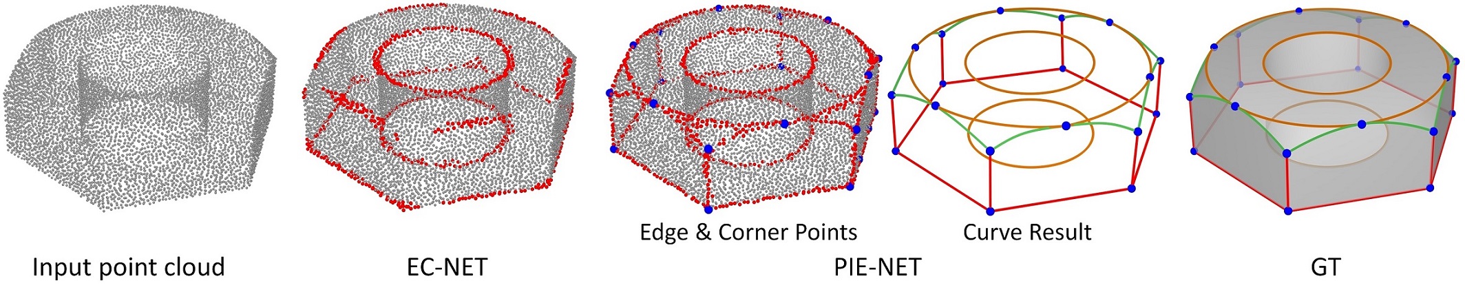
Figure 1: Our deep neural network, PIE-Net, is trained for parametric inference of edges from point cloud. It first detects edge and corner points, and then infers a collection of parametric curves representing edge features. In comparison, the only known deep method for this task only classifies edge points, and produces results that are inferior to ours both visually and quantitatively.

2 Related work

Literature on point-based graphics [5] is quite extensive and we refer readers to a recent survey [6]. Since the seminal work of Qi et. al. [7], there has been a proliferation of research on learning deep neural networks for 3D point cloud processing [8, 9, 10, 11, 12, 13, 14, 15, 16, 17]. We now focus on methods that are most closely related: \raisebox{-.75pt}{1}⃝ primitive inference, \raisebox{-.75pt}{2}⃝ consolidation, and \raisebox{-.75pt}{3}⃝ edge detection.

Parametric primitive inference

Parametric primitive fitting has been a long-standing problem in geometry processing. The detection or fitting of parametric feature curves (such as Bezier curves) in 3D point clouds has been extensively researched, where it is typically formulated in least squares form [18, 19, 20, 21]. Alternatively, one can use random RANSAC-type algorithms [22] to propose the parameters of primitives fitting a given point cloud. Many types of primitive shapes (planes, spheres, quadratic surfaces) have been considered and various applications have been explored – from 3D reconstruction and modeling [23, 24] to robotic grasping [25]. Besides predefined primitives, recent works also studied learning data-driven geometric priors for shape fitting [26, 27]. End-to-end models have been proposed for fitting cuboids [28], super-quadrics [29], and convexes [30, 31]. Li et al. [11] propose a supervised method to detect a variety of primitive patches at various scales. Similarly to our work, their network first predicts per-point properties, and later estimates primitives.

Edge-aware consolidation and reconstruction

Edge feature detection has been applied to enhance 3D reconstruction [32, 33, 34, 35]. Oztireli et al. [32] leverage MLS and robust estimators to automatically identify sharp features and preserve them in the resulting implicit reconstruction. Huang et al. [33] first computes normals reliably away from edges, and then progressively re-samples the point cloud towards edges leading to edge-preserving reconstruction. Edge detection has also been utilized to enhance RGBD reconstruction, where Liu et al. [35] propose to detect edges for the task of wire reconstruction from RGBD sequences. Consolidation has also been adopted in designing deep neural networks. Yu et al. [36] propose PU-Net for point cloud upsampling. It first learns per point features and then expands them with a multi-branch convolution unit. The expanded feature is then split to a multitude of features used to reconstruct a dense point set. EC-Net [10] proposes a deep edge-aware point cloud consolidation framework. The network is trained to regress and recover upsampled 3D points and point-to-edge distances. The reconstruction of surfaces with sharp edges has also recently been tackled by learnable sparse convex decomposition [31], but this method performs a feature-aware reconstruction as a holistic task.

Edge feature detection

Edge feature detection from point clouds relies on local geometric properties such as normals [37], curvatures [38], and feature anisotropy [39]. For example, Fleishman et al. [40] employ robust estimators to identify edge features, but shape analysis relies on moving least squares (MLS) to locally model the neighborhood of a point. Daniels et al. [41] extend this method to extract feature curves from noisy point clouds based on the reconstructed MLS surface. It is also possible to extract edge features via point cloud segmentation of these local properties [42, 43]. The closest work to ours is EC-Net [10], whose first phase consists of point classification and regression of per-point distances to the edge. Edge points are then detected as the points with a zero point-to-edge distance. To the best of our knowledge, EC-Net is the only prior work on feature edge estimation using deep learning and PIE-Net is the first technique that estimates parametric edge curves with an end-to-end trainable deep network.

3 Method

Figure 2: Pipeline – Our method treats parametric edge inference as a region proposal task. Given a point cloud, our network first detects edges and corners. Then, for each pair of corners, it performs curve proposal generation and selection to detect feature edges as a set of parametric curves.

The processing pipeline of Parametric Inference of Edges Network is summarized in Figure 2. Our technique treats point cloud curve inference as curve proposal process followed by selection, a technique inspired by image-based object detection pipelines [44].

Overview

Given a point cloud, a detection module first identifies edge and corner points (Section 3.1). Corners represent the start/end points of curves, or the locations where two curves touch. Pairs of corners are then given to a curve proposal module (Section 3.2) to identify the corresponding “edge points”, and finally generate a corresponding parametric open curve proposal. For closed curves, as they do not have a well defined start/end, we take inspiration from the Similarity Group Proposal Network [45], and regress the parameters of closed curves by first performing a clustering of the identified edge points, followed by curve fitting. Finally, a simple curve selection scheme merges all the curve proposals to generate the final fitting result.

Training data

We performed a statistical analysis over the ABC dataset [46], a large-scale CAD mechanical part dataset containing ground-truth annotations for edges and corner points. We found that the edges of the mechanical parts largely belong to three types, i.e., lines, circles, and B-spline curves, which account for more than 95$\%$ of the edges. We ignored the “ellipse” and “other” types due to their statistical insignificance. Therefore, we only focus on these three curve types in this paper, and filter out other types in the ground truth. For each ABC model, we sample it into a point cloud containing 8,096 points, via uniform point sampling. We then transfer the ground-truth annotations of the CAD models to the point clouds by nearest neighbor assignment.

Parameterization

Our method deals with three types of curves: lines, circles (open arcs plus full closed circles), and B-splines. We now describe the differentiable parameterization of the two latter curve types, where we note that a line segment can be formed by simply connecting two corner points. We parameterize circles as $\beta{=}(p_{1},p_{2},p_{3})$, where $p_{1}$, $p_{2}$, $p_{3}$ are any three points on the circle that are not collinear. We first transform $\beta{=}(p_{1},p_{2},p_{3})$ as $(n,c,r)$, where $n$ is the normal of the circle, and $c$ and $r$ are its center and radius. We then randomly sample points on the circle, and express them as a function of $\beta$. To achieve this, we draw $\alpha\in[0,2\pi]$, and generate random samples $p(\alpha|\beta){=}c+r(ucos(\alpha)+vsin(\alpha))$, where $u{=}p_{1}-c$ and $v{=}u\times n$. We parameterize B-Spline curves with four control points $\beta{=}\{p_{i}\}_{i=0}^{3}$. Given $B_{i,K}(\cdot)$ representing the $i$-th basis function of a $K$-th order B-spline, and $\alpha$ sampled uniformly in the $[0,1]$ range, we draw a uniform random sample as $p(\alpha|\beta){=}\Sigma_{i}{p_{i}B_{i,K}(\alpha)}$. Note that to ensure that $p(0|\beta){=}c_{1}$ and $p(1|\beta){=}c_{2}$, we employ quasi-uniform B-splines. We predict residuals as the displacement of the two intermediate control points $\{p_{i}\}_{i=1,2}$.

3.1 Point classification

To classify points in the input point cloud into edge and corners (plus the null class), we use a PointNet++ like architecture [47]. In particular, we devise two separate classification networks outputting edge vs. null and corner vs. null, respectively. The network predicts the probability of a point being on an edge $T_{e}$, or a corner $T_{c}$, or null otherwise, as well as the 3D offset vector $D_{e}$ that projects the point onto an edge, and the offset $D_{c}$ that projects the point onto a corner – these predictions are supervised by the ground truth labels $\hat{T}_{e}$ and $\hat{T}_{c}$, as well as the ground truth offsets $\hat{D}_{e}$ and $\hat{D}_{c}$. We then threshold the probabilities $T_{e}{>}\tau_{e}$ and $T_{c}{>}\tau_{c}$ to obtain a corresponding set of edge points $E{=}\{e_{i}\}_{\text{i=1}}^{M}$ and corner points $C{=}\{c_{i}\}_{\text{i=1}}^{N}$. We set the parameters $\tau_{e}{=}0.7$ and $\tau_{c}{=}0.9$ throughout our experiments. We optimize the multi-task loss $\mathcal{L}_{\text{detection}}{=}\mathcal{L}_{\text{edge}}{+}\mathcal{L}_{\text{corner}}$:

$$\mathcal{L}_{\text{edge}} =\mathcal{L}_{\text{cls}}(T_{e},\hat{T}_{e})+\hat{T}_{e}\cdot\lambda_{e}\mathcal{L}_{\text{reg}}(D_{e},\hat{D}_{e}),$$ (1)

$$\mathcal{L}_{\text{corner}} =\mathcal{L}_{\text{cls}}(T_{c},\hat{T}_{c})+\hat{T}_{c}\cdot\lambda_{c}\mathcal{L}_{\text{reg}}(D_{c},\hat{D}_{c}),$$ (2)

where for $\mathcal{L}_{\text{cls}}$, rather than traditional binary cross-entropy, we employ a focal loss [48] to deal with the pathological class imbalance in our dataset (the number of edge points is very small relative to the number of non-edge points). For $\mathcal{L}_{reg}$, we use the smooth $L_{1}$ loss as in [49, 44].

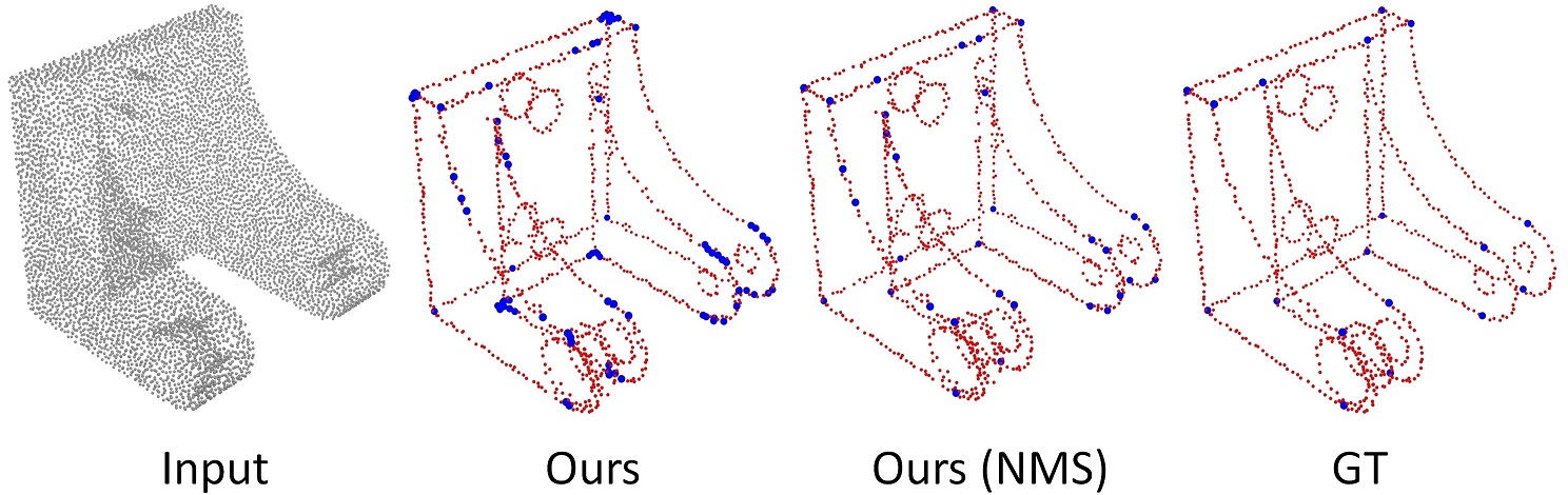
Figure 3: Point classification – We determine whether each point belongs to an edge or to a corner. We show the results of our method before and after NMS, as well as the corresponding ground truth.

Non-maximal suppression

At test time, we first classify corner points and regress the corresponding offset vectors. However, due to noise, several points may be mislabelled as corners in the proximity of a ground-truth corner, hence necessitating post-processing. To this end, we adopt a point-level Non-Maximal Suppression (NMS). After applying the offset to the detected corner points, we perform agglomerative clustering with a maximum intra-class distance threshold $\delta$; we use $\delta{=}0.05\ell$, with $\ell$ being the diagonal length of object bounding box. We then perform NMS within each cluster by selecting the corner with the highest classification probability; see Figure 3.

3.2 Open Curve proposal

PIE-Net performs a curve proposal for open curves and another for closed curves. Our open curve proposal generation leverages the fact that open curves connect two corner points, and makes the assumption that a corner pair can support at most one curve. Hence, given the set $C$ with $N$ corner points, we start by generating all $O(N^{2})$ corner point combinations and create corner pairs $\{\mathcal{P}_{i}{=}\{{c_{i}}_{1},{c_{i}}_{2}\}\>|\>{c_{i}}_{1},{c_{i}}_{2}\in C\}$. Each corner pair will correspond to a curve proposed by the curve proposal generation; see Figure 4. Given a pair $\mathcal{P}_{i}$, we need to identify points that should be associated to the corresponding curve. We first localize the search via a heuristic that only considers points in $E$ that lie within a sphere with center $({c_{i}}_{1}+{c_{i}}_{2})/2$, and radius $R{=}\|{c_{i}}_{1}-{c_{i}}_{2}\|/2$. Within this sphere, we then uniformly sample a subset $E^{o}_{i}$ that has a cardinality compatible with the input dimension of our multi-headed PointNet networks and feed $E^{o}_{i}$ to them; see Figure 4.

Losses

The network heads perform three different tasks, and are trained by three different losses. The first network head performs segmentation, determining whether a particular point belongs to the candidate curve. The second head performs classification, determining whether we need to generate a line, circle, or B-spline. The third head performs regression, identifying the parameters of the proposed curve. Note that the network outputs the parameters for all curve types and only those corresponding to the type output by the type classifier are regarded as the valid output. More formally:

$$\mathcal{L}_{\text{proposal}}=w_{\text{m}}\mathcal{L}_{\text{mask}}(M_{p},\hat{M}_{p})+w_{\text{c}}\mathcal{L}_{\text{cls}}(T_{p},\hat{T}_{p})+w_{\text{p}}\mathcal{L}_{\text{para}}(\beta),$$ (3)

where $M_{p}$ and $\hat{M}_{p}$ are the predicted / ground-truth classifications, $T_{p}$ and $\hat{T}_{p}$ are predicted / ground-truth curve types, and $\beta$ represents the predicted curve parameters. We set $w_{\text{m}}{=}1$, $w_{\text{c}}{=}1$, and $w_{\text{p}}{=}10$ throughout our experiments. Softmax cross-entropy is employed for both $\mathcal{L}_{\text{mask}}(\centerdot)$ and $\mathcal{L}_{\text{cls}}(\centerdot)$, while for regression:

$$\mathcal{L}_{\text{para}}=\hat{T}_{\text{circle}}\cdot\mathcal{L}_{\text{circle}}(\beta)+\hat{T}_{\text{line}}\cdot\mathcal{L}_{\text{line}}(\beta)+\hat{T}_{\text{spline}}\cdot\mathcal{L}_{\text{spline}}(\beta),$$ (4)

where $\hat{T}_{*}$ encodes the ground truth one-hot labels for the corresponding curve type, while $\mathcal{L}_{\text{*}}$ are Chamfer Distance losses measuring the expectation of Euclidean distance deviation between the curve having parameters $\beta$ and the ground truth. In order to compute expectations, we need to draw random samples from each curve type which are parametric in the degrees of freedom $\beta$.

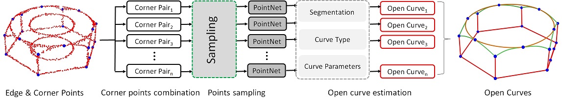
Figure 4: Open curve proposal – Given the collection of corners, we generate all possible corner pairs and propose an open curve connecting the pair of corners. In doing so, we predict the curve type, the parameters, and the subset of points corresponding to the proposed curve.

3.3 Closed curve proposal

Our closed curve proposal module is inspired by [45]. In particular, we first identify the subset of points belonging to closed curves via feature clustering, and then fit a closed curve to each proposed cluster, while simultaneously estimating the confidence of the fit; see Figure 5. Here we use the edge/corner classification described in Section 3.1 of the main paper. Note our method currently only handles curves with a circular profile, but it can be easily extended to other types of closed curves.

Clustering

We train an equivariant PointNet++ network to produce a point-wise feature $F(\cdot)$ for each of the $M$ input edge points. Based on such features, we then create a similarity matrix $S{\in}\mathbb{R}^{M\times M}$, where $S_{ij}{=}\|F(p_{i})-F(p_{j})\|_{2}$. We can then interpret each of the $M$ rows of $S$ as a proposal, and consider the set $C_{m}{=}\{j\text{ s.t. }S_{m,j}{<}\bar{S}\}$ as the edge points of the $m$-th proposal. $\bar{S}$ is a threshold to filter out the points attaining very different feature scores (i.e., they probably do not belong to the same curve). Potentially redundant proposals are dealt with in the selection phase of our pipeline, as described in Section 3.4.

Fitting

We take each proposal $C_{m}$, and regress the parameters $\beta$ of the corresponding curve, as well as its confidence $\gamma$. We parameterize each circle proposal via three points $\beta{=}\{p_{a}{+}\Delta_{a},p_{b}{+}\Delta_{b},p_{c}{+}\Delta_{c}\}$. We obtain $\{p_{a},p_{b},p_{c}\}$ by furthest point sampling in $C_{m}$ initialized with $p_{a}{=}p_{m}$. We then train a PointNet architecture with two fully-connected heads. The first head regresses the offsets $\{\Delta_{a},\Delta_{b},\Delta_{c}\}$, while the second head predicts $\gamma$.

Losses

We train our network to predict similarity matrices $S$ given ground truth $\hat{S}$, confidences $\Gamma{=}\{\gamma_{n}\}$ given ground truth $\hat{\Gamma}$, and a collection of points sampling the ground truth curve:

$$\mathcal{L}_{\text{closed}}=\mathcal{L}_{\text{sim}}(S,\hat{S})+\mathcal{L}_{\text{score}}(\Gamma,\hat{\Gamma})+\mathcal{L}_{\text{para}}(\beta).$$ (5)

Given that $\hat{S}_{ij}{=}0$ if points $p_{i}$ and $p_{j}$ belong to the same ground truth curve and $\hat{S}_{ij}{=}1$ otherwise, we supervise for similarity via:

$$\mathcal{L}_{\text{sim}}=\sum_{ij}S_{ij},$$ (6)

where

$$S_{ij}=\left\{\begin{array}[]{lll}\|F(p_{i})-F(p_{j})\|_{2},&{\hat{S}_{ij}=1}\\ \max\{0,K-\|F(p_{i})-F(p_{j})\|_{2}\},&{\hat{S}_{ij}=0}\end{array}\right.$$

where $F$ is point-wise feature computed with PointNet++. $K$ controls the dissimilarity between elements in different parts, which is set to $K{=}100$ in our experiments. For $\mathcal{L}_{\text{score}}(\cdot)$ we employ $L_{2}$ loss, where $\hat{\Gamma}$ is the segmentation confidence. Positive training examples come from seed points belonging to ground truth closed curves, and their IoU with ground truth segmentations is larger than $0.5$. Negative training examples are those with IoU smaller than $0.5$. For parameter regression, we minimize

$$\mathcal{L}_{\text{para}}=\hat{T}_{\text{circle}}\cdot\mathcal{L}_{\text{circle}}(\beta),$$ (7)

where $\hat{T}_{\text{circle}}$ is the ground truth one-hot labels, and $\mathcal{L}_{\text{circle}}(\cdot)$ is the Chamfer distance between the curve represented by $\beta$ and the ground truth. In particular, we first compute the circle according to the estimated $\beta$, and then sample it by points. We then compute the Chamfer distance between the estimated circle and its corresponding point-sampled ground-truth.

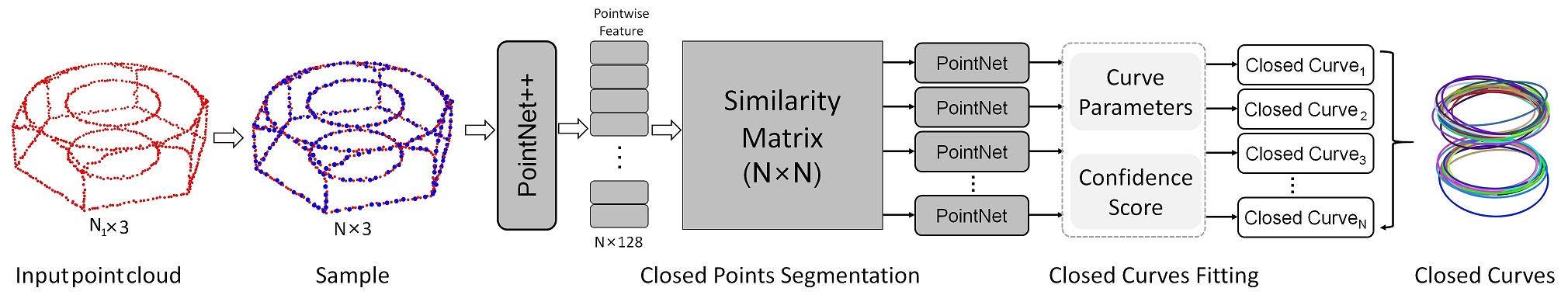
Figure 5: Closed curve proposal – We first identify the subset of points belonging to closed curves via feature-based clustering and then fit a closed curve to each cluster. The network outputs both curve parameters and confidence scores.

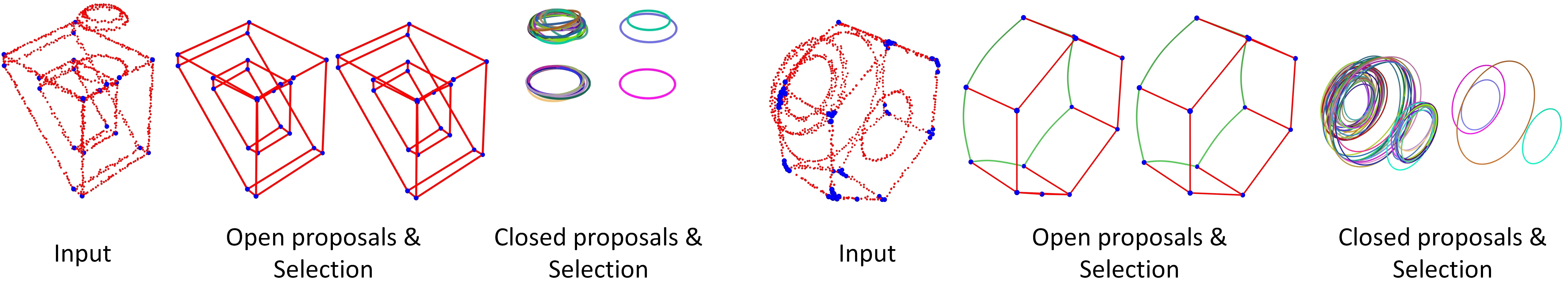
Figure 6: Proposal selection – The curves generated by open/closed proposals, and the ones that were accepted by our selection process.

3.4 Curve proposal selection

Similar to proposal-based object detection for images [44], the final stage of our algorithm is a non-differentiable process for redundant/invalid proposal filtering; see Figure 6. We adopt slightly different solutions for open and closed curves.

Open curve selection

Given the segmentations, i.e., a set of points associated with a curve (see Figure 5 in the main paper) corresponding with two proposals, we first measure overlap via $O(A,B)=max\{I(A,B)/A,I(A,B)/B\}$, where $I(A,B)$ is the cardinality of the intersection between the sets. We then merge the two candidates, if $O(A,B){>}\tau_{o}$ and retain the curve with larger cardinality, where we use $\tau_{o}{=}0.8$ as determined by hyper-parameter tuning.

Closed curve selection

The similarity matrix produces a closed-curve proposal for each of its $N$ rows. Even after discarding proposals with confidence score $\gamma_{n}{<}\tau_{\gamma}$, many are non-closed curves, or represent the same closed curve; see Figure 6. We perform agglomerative clustering for proposals when $\text{IoU}(A,B){>}\tau_{\text{iou}}$, and retain the proposal in the cluster with the highest confidence. We use $\tau_{\gamma}{=}0.6$ and $\tau_{\text{iou}}{=}0.6$ for all our experiments. Finally, for each closed segment, we select the best matching closed curve. Specifically, we use the Chamfer Distance to measure the matching score.

Figure 7: Results on edge and corner detection and parametric curve inference by PIE-Net.

4 Results and evaluation

In Figure 7, we show randomly selected qualitative results produced by PIE-Net, and generalization to object categories that are not part of our training dataset in Figure 10. We evaluate our network via ablation studies (Section 4.1), comparisons to both traditional and learned pipelines for edge detection (Section 4.2), and stress tests with respect to noise and sampling density (Section 4.3). To evaluate edge classification, we measure precision/recall and the IoU between predictions, while to evaluate the geometric accuracy of the reconstructed edges, we employ the Edge Chamfer Distance (ECD) introduced by [31]. Note that, differently from Chen et al. [31], we do not need to process the dataset to identify ground-truth edges, as these are provided by the dataset.

\begin{overpic}[width=433.62pt]{Images/radius_compare} \end{overpic}

	\raisebox{-.75pt}{1}⃝		\raisebox{-.75pt}{2}⃝		\raisebox{-.75pt}{3}⃝		\raisebox{-.75pt}{4}⃝
Metric	$R^{\prime}=1.5R$	$R^{\prime}=3R$	$\tau_{c}=0.8$	$\tau_{c}=0.95$	$\tau_{e}=0.6$	$\tau_{e}=0.8$	w/o $D_{e}$,$D_{c}$	PIE-Net
ECD $\downarrow$	0.0326	0.0824	0.0150	0.0144	0.0163	0.0149	0.0186	0.0136
IOU $\uparrow$	0.4386	0.2950	0.4875	0.5110	0.4356	0.4964	0.5017	0.5330
Precision $\uparrow$	0.5149	0.3244	0.5700	0.6032	0.5180	0.5975	0.5824	0.6219
Recall $\uparrow$	0.8570	0.8910	0.8415	0.8230	0.8340	0.8035	0.7849	0.8165

Figure 8: Ablation studies – We evaluate the qualitative (top) and quantitative (bottom) performance of our method across a number of metrics as we tweak: \raisebox{-.75pt}{1}⃝ the radius $R$ controlling the sampling heuristic, \raisebox{-.75pt}{2}⃝ the corner segmentation threshold $\tau_{c}$, \raisebox{-.75pt}{3}⃝ the edge segmentation threshold $\tau_{e}$, and \raisebox{-.75pt}{4}⃝ the edge and corner offsets $D_{e}$ and $D_{c}$. Recall for PIE-Net: $R^{\prime}{=}R$, $\tau_{c}{=}.9$, $\tau_{e}{=}.7$, and we use $D_{e},D_{c}$.

4.1 Ablation studies

Sphere radius – $R$

We validate the spherical sub-sampling heuristic introduced in Section 3.2. Note that we only consider values of $R^{\prime}$ strictly larger than the default setting, as otherwise we are guaranteed to miss edge features. Specifically, we set $R^{\prime}$ at $\times 1.5$ and $\times 3$ of the default $R$ – in the limit ($R^{\prime}{=}\infty$) we would consider the entire point cloud for each candidate corner-pair. Our analysis shows that as the sampled point cloud becomes larger and larger, it becomes more and more difficult to identify the right subset of points. This is because our sphere sampling heuristic also provides a hint of which curve needs to be sampled – the one whose corner points are touching the sphere.

Classification thresholds – $\tau_{c},\tau_{e}$

We also study curve generation performance as we vary how many corner points are accepted. Overall, the performance of the network is stable as we vary $\tau_{c}$, delivering the expected precision vs. recall trade-off. We find that curve generation quality slightly improves when we increase $\tau_{c}$, but as the threshold gets too large, the quality begins to decline as several corner points are filtered out, resulting in the absence of some feature curves. Analogous trade-offs are observed as we adjust the values of edge classification threshold $\tau_{e}$.

\begin{overpic}[width=433.62pt]{Images/all_edge_methods} \end{overpic}

	VCM			EAR			EC-Net	PIE-Net	PIE-Net
	$\tau{=}0.12$	$\tau{=}0.17$	$\tau{=}0.22$	$\tau{=}0.03$	$\tau{=}0.035$	$\tau{=}0.04$		RS
ECD $\downarrow$	0.0321	0.0430	0.0569	0.0679	0.0696	0.0864	0.0360	0.0137	0.0088
IOU $\uparrow$	0.2841	0.2854	0.2855	0.3404	0.3250	0.2844	0.3561	0.5976	0.6223
Precision $\uparrow$	0.3063	0.3244	0.3456	0.5560	0.4149	0.6523	0.4872	0.6816	0.6918
Recall $\uparrow$	0.8385	0.7644	0.6937	0.4820	0.5910	0.3578	0.5736	0.8319	0.8584

Figure 9: Comparisons to state-of-the-art methods – Qualitative (top) and quantitative (bottom) comparisons against point cloud with random sampling (RS) and edge detection techniques – VCM [50], EAR [51], and EC-Net [10].

4.2 Comparisons to the state-of-the-art

Two of the most classical, pre-deep learning, methods for point cloud edge detection are: \raisebox{-.75pt}{1}⃝ Merigot et al. [50], where edges are detected by thresholding the Voronoi Covariance Measure (VCM), and \raisebox{-.75pt}{2}⃝ Huang et al. [51], where edges are identified as part of an Edge-Aware Resampling (EAR) routine. We consider these two methods as representative of the state of the art, as both have been adopted in the point-set processing routines of the well known CGAL library [52]. As reported in Figure 9, our end-to-end method completely outperforms these classical baselines.

Voronoi Covariance Measure (VCM) [50]

We compute VCM for each point $\text{VCM}(p_{i})$, where we set offset radius to $0.5$ and convolution radius to $0.25$. These parameters were found by a parameter sweep evaluated over the test set of ABC [4]. We then consider a point to belong to an edge if $\text{VCM}(p_{i}){>}\tau$, and select three pareto-optimal thresholds $\tau{=}\{0.12,0.17,0.22\}$ for evaluation.

Edge Aware Resampling (EAR) [51]

This method first re-samples away from edges via anisotropic locally optimal projection (LOP), an operation that leaves gaps near sharp edges. We classify points as edges by detecting whether they fall within these gaps. This is achieved by computing the average distance $D_{10}(p_{i})$ to the ten nearest neighbors – we consider a point to belong to an edge if $D_{10}(p_{i})>\tau$. We report the results for $\tau=\{0.03,0.035,0.04\}$ – the best performing thresholds as selected by a dense sweep in the $[0.01\dots 0.05]$ range as suggested in the paper. As illustrated in Figure 9, our end-to-end method performs significantly better, as immediately quantified by the fact that ECD is an order of magnitude larger than the one reported for PIE-Net.

Edge-Aware Consolidation Network (EC-Net) [10]

We train EC-Net on our dataset, not the author’s dataset [10] as it only contained 24 CAD models with manually annotated edges, while ABC contains more than a million models. The comparison results demonstrate how PIE-Net achieves significantly better performance; see Figure 9. In particular, our qualitative analysis revealed how EC-Net struggles in capturing areas with weak-curvature, as well as short edges.

In Figure 10, we show additional qualitative comparison results on novel object categories such as tables, chairs, and vases, etc., which are not part of the ABC training set. These results were obtained using the same methods and trained networks as those that produced Figure 9. The point cloud inputs were obtained by uniform sampling on the original mesh shapes, which are shown in Figure 10 to reveal the edge features; there were no GT edges associated with these shapes.

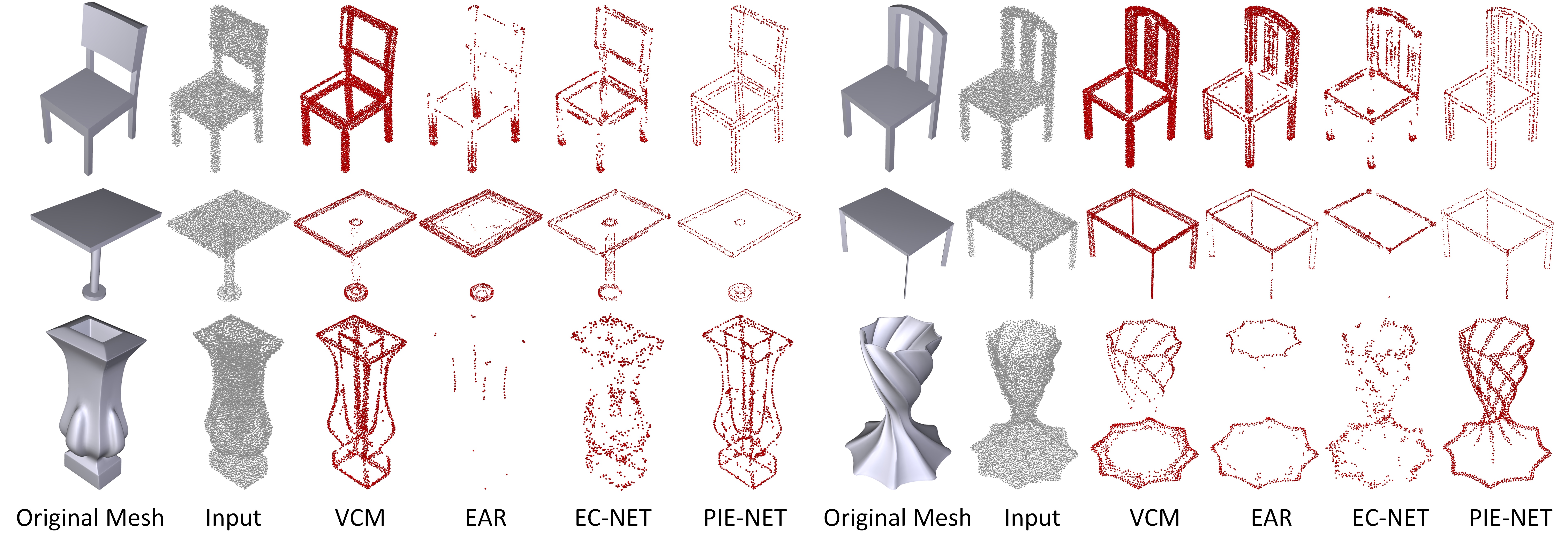
Figure 10: Generalization to novel object categories – While PIE-Net is trained on CAD models of mechanical assemblies from the ABC dataset [46], our edge detector is immediately applicable to 3D point clouds of general 3D objects and consistently outperforms VCM, EAR, and EC-Net.

\begin{overpic}[width=433.62pt]{Images/noise_and_sparse} \end{overpic}

Metric	$X=0.05$	$X=0.02$	$X=0.01$	$X=0.00$	$P$=1,024	$P$=2,048	$P$=4,096	$P$=8,096
ECD $\downarrow$	0.0924	0.0261	0.0159	0.0088	0.0473	0.0251	0.0185	0.0159
IOU $\uparrow$	0.5037	0.5905	0.6049	0.6223	0.4187	0.4972	0.5843	0.6049
Precision $\uparrow$	0.5973	0.6364	0.6672	0.6918	0.4985	0.5673	0.6549	0.6672
Recall $\uparrow$	0.7781	0.8385	0.8691	0.8584	0.7936	0.8445	0.8344	0.8691

Figure 11: Network behavior with respect to noise and sampling density – We show the qualitative (top) and quantitative (bottom) performance of PIE-Net on input point clouds degraded by noise of different magnitudes: $X{=}\{0.05,0.02,0.01,0\}$ or sampled at a reduced density: with $P$ going from 8,096 down to 1,024. All the numbers in boldface outperform VCM, EAR, and EC-Net without added noise or reduced point density; see the table in Figure 9 for reference.

4.3 Stress tests

Random Sampling (RS)

We sampled 100K points uniformly over each CAD shape, and then sub-sampled $8,096$ points non-uniformly via random sampling. We re-trained and re-tested PIE-Net on the new point clouds, keeping all other settings unchanged. The performance is reported in Figure Figure 9. As we can see, while there is a slight performance degradation, they are quite comparable to original and still outperform all performance statistics obtained by VCM, EAR, and EC-Net, except for one case, VCM with $\tau=0.12$, which yielded a recall of $0.8385$, but it is paired with a very low precision of only $0.3063$.

Point cloud noise

We stress test PIE-Net by increasing the level of noise. Specifically, we randomly apply different perturbations to the point samples along the surface normal direction with a scale factor in the $[1.0-X,1.0+X]$ range, where we tested four values of $X{=}\{0,0.01,0.02,0.05\}$. In each case, the network was trained with the noise-added data. Figure 11 shows some visual results and quantitative measures. As we can observe, our network, even when trained with noisy data, can still out-perform VCM, EAR, and EC-Net when they are tested on or trained on clean data.

Point density

We also train PIE-Net on point clouds at a reduced density. Specifically, for each CAD shape, we sampled a different number ($P$) of points to verify whether our network could handle the sparser point clouds, where $P{=}\{\text{8,096},\text{4,096},\text{2,048},\text{1,024}\}$. Results in Figure 11 reveal a similar trend as from the previous stress test. Namely, our network, when trained on sparser point clouds, can still outperform VCM, EAR, and EC-Net when they are tested on or trained on data at full resolution (8,096 points).

4.4 Timing

For all the results shown in the paper, the average running time is about $0.5$ second for point classification and 3 seconds for curve generation, per point cloud. In comparison, the average running times for point classification by VCM, EAR, and EC-Net are $5.5$, $4.0$, and $0.8$ seconds, respectively – they are all slower than PIE-Net. Training times for point classification,the open and closed curve proposal networks were about $23$, $12$, and $8$ hours, respectively, for $100$ epochs, on an NVIDIA TITIAN X GPU.

5 Conclusion

The detection of edge features in images has been shown to play a fundamental role in low-level computer vision — for example, the first layers in deep CNNs have been shown to be nothing but edge detectors. Notwithstanding, limited work to detect features of visual importance exists in 3D computer vision. With this objective, we present PIE-Net, a deep neural network which is trained to extract parametric curves from a point cloud that compactly describe its edge features. We demonstrate that a region proposal network architecture can already significantly outperform the state-of-the-art, which includes both traditional (non-learning) methods, and a recently developed deep model [10], the only other learning-based edge-point classifier, to the best of our knowledge.

Our contribution does not lie in merely surpassing the state-of-the-art from traditional graphics and geometry processing techniques. More importantly, we are introducing a new learning problem to the machine learning community, as well as defining the corresponding challenge for the recently published ABC dataset [4]. We also show that, yet again, networks can perform excellently even without resorting to excessive amounts of domain-specific (i.e., differential geometry) knowledge, as the only domain knowledge we assume is a simple curve parameterization.

paragraphtocFuture works (learning) From an architectural perspective, it would be natural to consider self-attention mechanisms to remove the need for ad-hoc solutions ($E^{o}_{i}$ in Section 3.2), as well as to employ deep representations of curves rather than explicit ones [atlasnet, gadelha2020dmp]. Integrating our edge detector with current deep models for 3D reconstruction [atlasnet, Matryoshka], scan/shape completion [park2019deepsdf, DBLP:journals/corr/DaiCSHFN17], and novel shape synthesis [3DGAN, chen2018implicit_decoder] may be the key missing ingredient which would significantly improve their results in terms of high-frequency geometric details.

Future works (geometry)

Our current method still has several technical limitations. The first is related to the current method’s inability to distinguish between close-by detected features. For example, as we generate open curve proposals based on corner pairs, for very short edges, the two corner points can be close to each other, and the network might assume that there is no connectivity between the two corner pairs. Also, our method cannot deal with scenarios where multiple curves connect two corners, or when the curve connecting the corners is (partially) outside the sphere associated with corners. We have not explored the full potential of a learning-based edge detector in handling significant noise and missing data. Another avenue for future investigation would be to transfer or extend our learning framework to handle large-scale 3D scenes.

Broader impact

We introduce a methodology that can benefit a range of current and new applications, from 3D data acquisition to object recognition. On the broader societal level, this work remains largely academic in nature, and does not pose foreseeable risks regarding defense, security, and other sensitive fields.

References

- [1] Guerrero, P., Y. Kleiman, M. Ovsjanikov, et al. PCPNET: Learning local shape properties from raw point clouds. In Computer Graphics Forum (Proc. of Eurographics), vol. 37, pages 75–85. 2018.
- [2] Wang, P.-S., Y. Liu, X. Tong. Mesh denoising via cascaded normal regression. ACM Trans. on Graphics, 35(6):232:1–232:12, 2016.
- [3] Yu, L., X. Li, C.-W. Fu, et al. PU-Net: Point cloud upsampling network. In Proc. IEEE Conf. on Computer Vision & Pattern Recognition. 2018.
- [4] Koch, S., A. Matveev, Z. Jiang, et al. Abc: A big cad model dataset for geometric deep learning. In Proc. IEEE Conf. on Computer Vision & Pattern Recognition. 2019.
- [5] Gross, M., H. Pfister. Point-Based Graphics. Morgan Kaufmann, 2007.
- [6] Berger, M., A. Tagliasacchi, L. Seversky, et al. A survey of surface reconstruction from point clouds. Computer Graphics Forum, 36:301––329, 2017.
- [7] Qi, C. R., H. Su, K. Mo, et al. Pointnet: Deep learning on point sets for 3D classification and segmentation. In Proceedings of the IEEE Conference on Computer Vision and Pattern Recognition, pages 652–660. 2017.
- [8] Guo, Y., H. Wang, Q. Hu, et al. Deep learning for 3d point clouds: A survey. arXiv preprint arXiv:1912.12033, 2019.
- [9] Duan, C., S. Chen, J. Kovacevic. 3d point cloud denoising via deep neural network based local surface estimation. In ICASSP 2019-2019 IEEE International Conference on Acoustics, Speech and Signal Processing (ICASSP), pages 8553–8557. IEEE, 2019.
- [10] Yu, L., X. Li, C.-W. Fu, et al. EC-Net: an edge-aware point set consolidation network. In Proc. Euro. Conf. on Computer Vision, pages 398–414. 2018.
- [11] Li, L., M. Sung, A. Dubrovina, et al. Supervised fitting of geometric primitives to 3d point clouds. In Proceedings of the IEEE Conference on Computer Vision and Pattern Recognition, pages 2652–2660. 2019.
- [12] Su, H., V. Jampani, D. Sun, et al. Splatnet: Sparse lattice networks for point cloud processing. In Proceedings of the IEEE Conference on Computer Vision and Pattern Recognition, pages 2530–2539. 2018.
- [13] Graham, B., M. Engelcke, L. van der Maaten. 3d semantic segmentation with submanifold sparse convolutional networks. In Proceedings of the IEEE Conference on Computer Vision and Pattern Recognition, pages 9224–9232. 2018.
- [14] Yu, F., K. Liu, Y. Zhang, et al. Partnet: A recursive part decomposition network for fine-grained and hierarchical shape segmentation. In Proceedings of the IEEE Conference on Computer Vision and Pattern Recognition. 2019.
- [15] Yi, L., H. Huang, D. Liu, et al. Deep part induction from articulated object pairs. ACM Transactions on Graphics (TOG), 37(6):209, 2019.
- [16] Wang, X., B. Zhou, Y. Shi, et al. Shape2motion: Joint analysis of motion parts and attributes from 3d shapes. In Proceedings of the IEEE Conference on Computer Vision and Pattern Recognition, pages 8876–8884. 2019.
- [17] Chen, D. Z., A. X. Chang, M. Nießner. Scanrefer: 3d object localization in rgb-d scans using natural language. arXiv preprint arXiv:1912.08830, 2019.
- [18] Wang, W., H. Pottmann, Y. Liu. Fitting b-spline curves to point clouds by curvature-based squared distance minimization. ACM Transactions on Graphics (ToG), 25(2):214–238, 2006.
- [19] Park, H., J.-H. Lee. B-spline curve fitting based on adaptive curve refinement using dominant points. Computer-Aided Design, 39(6):439–451, 2007.
- [20] Flöry, S., M. Hofer. Constrained curve fitting on manifolds. Computer-Aided Design, 40(1):25–34, 2008.
- [21] Zheng, W., P. Bo, Y. Liu, et al. Fast b-spline curve fitting by l-bfgs. Computer Aided Geometric Design, 29(7):448–462, 2012.
- [22] Schnabel, R., R. Wahl, R. Klein. Efficient ransac for point-cloud shape detection. Computer Graphics Forum, 26(2):214–226, 2007.
- [23] Sanchez, V., A. Zakhor. Planar 3d modeling of building interiors from point cloud data. In 2012 19th IEEE International Conference on Image Processing, pages 1777–1780. IEEE, 2012.
- [24] Wang, J., K. Xu. Shape detection from raw lidar data with subspace modeling. IEEE transactions on visualization and computer graphics, 23(9):2137–2150, 2016.
- [25] Gallardo, L. F., V. Kyrki. Detection of parametrized 3-d primitives from stereo for robotic grasping. In 2011 15th International Conference on Advanced Robotics (ICAR), pages 55–60. IEEE, 2011.
- [26] Remil, O., Q. Xie, X. Xie, et al. Surface reconstruction with data-driven exemplar priors. Computer-Aided Design, 88:31–41, 2017.
- [27] Wang, R., L. Liu, Z. Yang, et al. Construction of manifolds via compatible sparse representations. ACM Transactions on Graphics (TOG), 35(2):14, 2016.
- [28] Tulsiani, S., H. Su, L. J. Guibas, et al. Learning shape abstractions by assembling volumetric primitives. In Proceedings of the IEEE Conference on Computer Vision and Pattern Recognition, pages 2635–2643. 2017.
- [29] Paschalidou, D., A. O. Ulusoy, A. Geiger. Superquadrics revisited: Learning 3d shape parsing beyond cuboids. In Proceedings of the IEEE Conference on Computer Vision and Pattern Recognition, pages 10344–10353. 2019.
- [30] Deng, B., K. Genova, S. Yazdani, et al. Cvxnets: Learnable convex decomposition. arXiv preprint, 2019.
- [31] Chen, Z., A. Tagliasacchi, H. Zhang. Bsp-net: Generating compact meshes via binary space partitioning. arXiv preprint, 2019.
- [32] Öztireli, A. C., G. Guennebaud, M. Gross. Feature preserving point set surfaces based on non-linear kernel regression. In Computer Graphics Forum, vol. 28, pages 493–501. Wiley Online Library, 2009.
- [33] Huang, H., S. Wu, M. Gong, et al. Edge-aware point set resampling. ACM transactions on graphics (TOG), 32(1):9, 2013.
- [34] Zhou, Q.-Y., V. Koltun. Depth camera tracking with contour cues. In Proceedings of the IEEE Conference on Computer Vision and Pattern Recognition, pages 632–638. 2015.
- [35] Liu, L., N. Chen, D. Ceylan, et al. Curvefusion: reconstructing thin structures from rgbd sequences. In SIGGRAPH Asia 2018 Technical Papers, page 218. ACM, 2018.
- [36] Yu, L., X. Li, C.-W. Fu, et al. Pu-net: Point cloud upsampling network. In Proceedings of the IEEE Conference on Computer Vision and Pattern Recognition, pages 2790–2799. 2018.
- [37] Weber, C., S. Hahmann, H. Hagen. Sharp feature detection in point clouds. In 2010 Shape Modeling International Conference, pages 175–186. IEEE, 2010.
- [38] Hackel, T., J. D. Wegner, K. Schindler. Contour detection in unstructured 3d point clouds. In Proceedings of the IEEE Conference on Computer Vision and Pattern Recognition, pages 1610–1618. 2016.
- [39] Gumhold, S., X. Wang, R. S. MacLeod. Feature extraction from point clouds. In IMR. Citeseer, 2001.
- [40] Fleishman, S., D. Cohen-Or, C. T. Silva. Robust moving least-squares fitting with sharp features. In ACM transactions on graphics (TOG), vol. 24, pages 544–552. ACM, 2005.
- [41] Daniels Ii, J., T. Ochotta, L. K. Ha, et al. Spline-based feature curves from point-sampled geometry. The Visual Computer, 24(6):449–462, 2008.
- [42] Demarsin, K., D. Vanderstraeten, T. Volodine, et al. Detection of closed sharp edges in point clouds using normal estimation and graph theory. Computer-Aided Design, 39(4):276–283, 2007.
- [43] Feng, C., Y. Taguchi, V. R. Kamat. Fast plane extraction in organized point clouds using agglomerative hierarchical clustering. In 2014 IEEE International Conference on Robotics and Automation (ICRA), pages 6218–6225. IEEE, 2014.
- [44] Ren, S., K. He, R. Girshick, et al. Faster r-cnn: Towards real-time object detection with region proposal networks. In Advances in neural information processing systems, pages 91–99. 2015.
- [45] Wang, W., R. Yu, Q. Huang, et al. Sgpn: Similarity group proposal network for 3d point cloud instance segmentation. In Proceedings of the IEEE Conference on Computer Vision and Pattern Recognition. 2018.
- [46] Koch, S., A. Matveev, Z. Jiang, et al. Abc: A big cad model dataset for geometric deep learning. In Proceedings of the IEEE Conference on Computer Vision and Pattern Recognition, pages 9601–9611. 2019.
- [47] Qi, C. R., L. Yi, H. Su, et al. Pointnet++: Deep hierarchical feature learning on point sets in a metric space. In Advances in neural information processing systems, pages 5099–5108. 2017.
- [48] Lin, T.-Y., P. Goyal, R. Girshick, et al. Focal loss for dense object detection. In Proceedings of the IEEE international conference on computer vision, pages 2980–2988. 2017.
- [49] Girshick, R. Fast r-cnn. In Proceedings of the IEEE international conference on computer vision, pages 1440–1448. 2015.
- [50] Merigot, Q., M. Ovsjanikov, , et al. Voronoi-based curvature and feature estimation from point clouds. IEEE Trans. Visualization & Computer Graphics, 17(6):743–756, 2011.
- [51] Huang, H., S. Wu, M. Gong, et al. Edge-aware point set resampling. ACM Trans. on Graphics, 32:9:1–9:12, 2013.
- [52] Alliez, P., S. Giraudot, C. Jamin, et al. Point set processing. In CGAL User and Reference Manual. CGAL Editorial Board, 5.0 edn., 2019.