Subject-Aware Contrastive Learning for Biosignals

Abstract

Datasets for biosignals, such as electroencephalogram (EEG) and electrocardiogram (ECG), often have noisy labels and have limited number of subjects ($<$100). To handle these challenges, we propose a self-supervised approach based on contrastive learning to model biosignals with a reduced reliance on labeled data and with fewer subjects. In this regime of limited labels and subjects, intersubject variability negatively impacts model performance. Thus, we introduce subject-aware learning through (1) a subject-specific contrastive loss, and (2) an adversarial training to promote subject-invariance during the self-supervised learning. We also develop a number of time-series data augmentation techniques to be used with the contrastive loss for biosignals. Our method is evaluated on publicly available datasets of two different biosignals with different tasks: EEG decoding and ECG anomaly detection. The embeddings learned using self-supervision yield competitive classification results compared to entirely supervised methods. We show that subject-invariance improves representation quality for these tasks, and observe that subject-specific loss increases performance when fine-tuning with supervised labels.

1 Introduction

Biosignal classification can lead to better diagnosis and understanding of our bodies and well-being. For example, medical experts can monitor health conditions, such as epilepsy [1] or depression [2], using brain electroencephalography (EEG) data. In addition, electrocardiograms (ECG) give insight to cardiac health and can also indicate stress [3].

Time-series biosignals can be non-invasively and continuously measured. However, labeling these high-dimensional signals is a labor-intensive and time-consuming process, and assigning labels may introduce unintended biases. We propose to use self-supervised learning methods to extract meaningful representations from these high-dimensional signals without the need of labels. In this work, we make the following contributions:

Apply self-supervised learning to biosignals.

Speech and vision data are processed by the human senses of hearing and sight. Whereas, biosignals can be the result of processing this information along with other complex biological mechanisms. Information may be obscured or lost when measuring these processes with the resulting time-series signals. Thus, it is unclear whether the same techniques used to learn representations for language and vision domains are effective for biosignals. In this work, we demonstrate the effectiveness of contrastive loss for self-supervised learning for biosignals. This approach requires the development and assessment of augmentation techniques and the consideration of intersubject variability, the signal variations from subject to subject.

Develop data augmentation techniques for biosignals.

Data transformation algorithms help increase the information content in the learned embeddings for desired downstream tasks. In this work, we develop domain-inspired augmentation techniques. For example, the power in certain EEG frequency bands has been shown to be highly correlated with different brain activities. Thus, we use frequency-based perturbations to augment the signal. We find that temporal specific transformations (cutout and delay) are the most effective transformations for representation learning followed by signal mixing, sensor perturbations (dropout and cutout), and bandstop filtering.

Integrate subject awareness into the self-supervised learning framework.

Inter-subject variability poses a challenge when performing data-driven learning with a small number of subjects. Subject-specific features are an integral part of biosignals, and the knowledge that the biosignals are from different subjects is a “free” label. We investigate two solutions to integrate this feature into the self-supervised learning framework: (1) using subject-specific distributions to compute the contrastive loss, and (2) promoting subject invariance through adversarial training. Experimental results show that promoting subject invariance increases classification performance when training with a small number of subjects. Both approaches yield weight initializations that are effective in fine-tuning with supervised labels.

2 Related Work

Representation learning for temporal signals.

Temporal signals introduce an additional dimension to exploit for self-supervised learning. Previous work used temporal dynamics such as temporal ordering [4, 5] or temporal prediction [6]. Designing and including multiple pretext tasks [7] has been shown to be effective in representation learning for both EEG [8] and ECG signals [9].

Alternatively, representation learning can be performed through clustering with contrastive learning [10, 11, 12, 13]. In this framework, a single instance is clustered with different perturbations of itself while pushing all other instances away in the embedding space. The non-stationary property of biosignals can be exploited where further time instances of the same data stream can be considered as negative training examples [14]. Here, we take the concepts proposed by Hyvärinen and Morioka [14] that was demonstrated for magnetoencephalography (MEG), and we apply the contrastive learning framework [13] for time-series biosignals. This application requires careful design of appropriate data transformations and consideration of intersubject variability.

Incorporating subject-based information.

Intersubject variability can be interpreted as a different domain for each subject. The domain shift from subject to subject can be modeled and corrected with adversarial training [15], as shown for neural signals recorded with multi-electrode arrays [16]. The model can also be promoted to learn domain-invariant features [17, 18] as demonstrated for regularizing a classifier for EEG processing [19]. In our work, we introduce subject-invariance into the contrastive learning framework and investigate the impact using the learned representations in downstream tasks.

3 Methods

Self-supervised learning is performed using contrastive learning with data transformation techniques [10, 12, 13]. First, contrastive learning framework is described with the proposed addition of subject awareness to address intersubject variability. Next, specific transformation techniques for training are designed and introduced to more effectively learn biosignal representations. Lastly, the proposed approach is applied to downstream tasks as described in the next section.

3.1 Model and Contrastive Loss Function

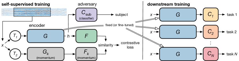
Figure 1: Method overview. An encoder $G$ is trained using self-supervised training (left) with an adversarial subject identifier to minimize subject-specific content. Alternatively, subject-awareness can be introduced through subject-specific contrastive loss. The resulting encoder can then be applied for different downstream tasks by attaching a classification model (right).

The method is summarized in Fig. 1. Encoder $G(T_{1}(x_{i}))$ with parameters $\theta_{G}$ encodes data sample $x_{i}$ with transformation $T_{1}$ to latent representation $h_{i}$. During self-supervised training, $h_{i}$ is passed through model $F(h_{i})$ with parameters $\theta_{F}$ to yield $q_{i}$: $q_{i}=F\left(G\left(T_{1}\left(x_{i}\right)\right)\right)$. Copies of $G$ and $F$ as $G_{k}$ and $F_{k}$ are used to generate $k_{i}$ from $x_{i}$ with transformation $T_{2}$: $k_{i}=F_{k}(G_{k}(T_{2}(x_{i}))$. The models $G_{k}$ and $F_{k}$ are updated with momentum [12]. Both $q_{i}$ and $k_{i}$ are normalized to unit L2-norm.

The models are trained to maximize the mutual information between $T_{1}(x_{i})$ and $T_{2}(x_{i})$ for any $T_{1}$ and $T_{2}$. The mutual information maximization is estimated with InfoNCE [20, 6]:

$$\ell_{i}=-\log{\frac{\exp{\left(q_{i}^{T}k_{i}/\tau\right)}}{\sum_{j=0}^{N}\exp{\left(q_{i}^{T}k_{j}/\tau\right)}}},$$ (1)

where the inner product $q_{i}^{T}k_{i}$ is used as a similarity metric and $\tau$ is a learnable temperature parameter. In Eq. 1, $q_{i}^{T}k_{i}$ is contrasted against the inner product of $q_{i}$ and $N-1$ negative examples. The momentum update of $G_{k}$ and $F_{k}$ enables the use of negative examples from previous batches to increase the number of negative examples [12].

This loss focuses on features that differentiate each time segment from other time segments. With the variability in how the sensors are setup and how the signals behave for each subject, the learned embeddings will be dominated by subject-specific characteristics. To promote the extraction of subject-invariant features, we apply adversarial training [21, 18]. A classifier $C_{\textrm{sub}}$ is trained to predict the identity of the subject of each example based on latent vector $h_{i}$: $C_{\textrm{sub}}(h_{i})=C_{\textrm{sub}}(G(x_{i}))$. The $j$-th element, $C^{j}_{\textrm{sub}}(h_{i})$, corresponds to the probability of $h_{i}$ being from subject $j$. This model is trained with a fixed encoder $G$ using cross entropy loss:

$$\ell_{\textrm{sub},i}=-\sum_{j=0}^{N_{\textrm{sub}}-1}\mathbbm{1}_{[j=s_{i}]}\log C^{j}_{\textrm{sub}}(G(x_{i})),$$ (2)

where $N_{\textrm{sub}}$ is the number of subjects, $s_{i}$ is the subject number of example $i$, and $\mathbbm{1}_{[j=s_{i}]}$ is an indicator function with a value of 1 when $j=s_{i}$. The encoder $G$ is encouraged to confuse this subject classifier by using a fixed $C_{\textrm{sub}}$ to regularize the training of $G$ and $F$ with the regularization term of:

$$r_{\textrm{sub},i}=-\sum_{j=0}^{N_{\textrm{sub}}-1}\mathbbm{1}_{[j=s_{i}]}\log\left(1-C^{j}_{\textrm{sub}}(G(x_{i}))\right).$$ (3)

The final loss functions become:

$$\operatorname*{argmin}_{F,G}\mathbbm{E}_{i}\left[\ell_{i}+\lambda r_{\textrm{sub},i}\right],\textrm{and }\operatorname*{argmin}_{C}\mathbbm{E}_{i}\left[\ell_{\textrm{sub},i}\right],$$ (4)

where $\lambda$ is a tunable hyperparameter. Unless specified, $\lambda$ was set to 1 in the experiments. We refer to this approach as subject-invariant self-supervised learning since the embedding is regularized to minimize subject-based information. For multi-session measurements, the differences in sensor setup for the same subject will also be a factor but can be treated as a separate subject with this formulation.

Subject information can also be incorporated in the negative sampling procedure when computing the contrastive loss. The noise estimation can be based only on the data distribution of a single subject. This procedure focuses the loss on differences in time for a single subject, and does not consider differences between subjects. We refer to this approach as subject-specific self-supervised learning. We refer to self-supervised learning (SSL) without subject-awareness as base SSL.

3.2 Data Transformations for Biosignals

Two random transformations are applied to each training example $x_{i}$: $y_{i,1}=T_{1}(x_{i})$ and $y_{i,2}=T_{2}(x_{i})$. We investigate a number of transformations in the context of biosignals (Fig. 2):

• Temporal cutout: a random contiguous section of the time-series signal (cutout window) is replaced with zeros [22];

• Temporal delays: the time-series data is randomly delayed in time;

• Noise: independent and identically distributed Gaussian noise is added to the signal;

• Bandstop filtering: the signal content at a randomly selected frequency band is filtered out using a bandstop filter; and

• Signal mixing: another time instance or subject data is added to the signal to simulate correlated noise.

These signals are collected from physical sensors that are dispersed in space. For EEG signals, multiple electrodes are placed around the surface of the head. These spatial locations can be used to help augment the data with domain-specific transformations:

• Spatial rotation: the data is rotated in space [23];

• Spatial shift: the data is shifted in space;

• Sensor dropout: a random subset of sensors is replaced with zeros; and

• Sensor cutout: sensors in a small region of space are replaced with zeros.

For random bandstop filters, we designed a fixed low-pass filter using a hamming window with 31 coefficients. This filter was first converted to a bandpass filter by modulating the filter using a cosine function with a random phase selected with uniform probability. The signal was bandpassed using this filter and subtracted from the original signal. Radial basis function interpolation was used to perform the spatial rotation and spatial shift transformations.

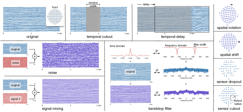
Figure 2: Data transformations for augmentations demonstrated for EEG signals. The original data input is shown in the upper left corner. Multi-channel biosignals can be further augmented with spatial perturbations (right column). All augmentations were used for our experiments with the exception of spatial rotation/shift and sensor cutout for ECG.

4 Experiments and Results

All experiments were performed using PyTorch (v1.4.0) [24]. One-dimensional ResNet models [25] with ELU activation and batch normalization [26] were used for encoders $G$ with slightly different parameters for each application (see Appendix for details). Model $F$ consisted of a 4-layer fully-connected network with 128 dimensions at each stage and 64 dimensions at the output. Unless specified, Adam optimizer [27] was used with a learning rate of 1e-4. Self-supervised learning with momentum was applied with a $k_{i}$ history of 24k elements and an update momentum of 0.999. On an NVIDIA Tesla V100 card with 32GB, this training took 47.8–54.6 hours for the EEG dataset and 33.7–39.2 hours for the ECG dataset. Linear classification using logistic regression with weight decay of 0.01 was performed to evaluate the quality of the learned embeddings. Results were reported as mean $\pm$ standard deviation across 10 trials, each performed with a different random seed.

4.1 EEG: PhysioNet Motor Imagery Dataset

Electrical neural activity can be non-invasively recorded using electrodes placed on the scalp with EEG. Being able to derive meaningful representations from these signals will enable further understanding of the brain. However, these signals are difficult to interpret and label. Therefore, we applied our approach to the PhysioNet motor movement/imagery dataset [28, 29, 30]. Data were recorded from 109 volunteers where each subject was asked to perform imagined motor tasks: closing the right fist, closing the left fist, closing both fists, and moving both feet. Each task lasted for $\sim$4 sec and was also performed with actual movement. Following previous work [31], we excluded data from 3 volunteers due to inconsistent timings. During the experiment, 64-channel EEG data were recorded at 160 Hz using the BCI2000 system [29]. We re-referenced the raw data using the channel average, and normalized the data by the mean and standard deviation of the training dataset.

Experimental Setup.

Encoder $G$ (288k parameters, model details in Appendix) was trained using self-supervised learning with data from 90 subjects. For each recording (both imagined and action trials), a time window was randomly selected as the input to $G$. A 256-dimensional embedding vector was produced by the encoder for every 320 samples (2 sec). Self-supervised training was performed with a batch size of 400 and 270k steps (or 54k steps if only one augmentation or none was applied).

A logistic-regression linear classifier was trained on top of the frozen $G$ model using the class labels and data from the same 90 subjects for the imagined trials only. Each example was a 2-sec window of data selected 0.25 sec after the start of each trial to account for response time after the cue. The resulting classifier and encoder $G$ was then evaluated on 16 held-out subjects. This experimental setup is referred as intersubject testing. Two downstream task setups were performed: (1) 2-class problem of determining imagined right fist or left fist movements based on the EEG signal, and (2) 4-class problem of determining imagined right fist, left fist, both fists, or both feet movements. Classifiers were trained using a learning rate of 1e-3 and batch size of 256 for 2k epochs.

Impact of Transformation.

To understand the effectiveness of each transformation (e.g. temporal cutout, random temporal delay) and the associated parameter (e.g. temporal cutout window, maximum temporal delay), a single transformation type was applied for $T_{2}$ during the self-supervised training, and the identity transform was used for $T_{1}$. Afterwards, the learned encoder $G$ was evaluated by training a linear classifier on top of the frozen network for the 4-class task.

Temporal cutout was the most effective transformation followed by temporal delay and signal mixing (Table 1). The effect of temporal transformations was the promotion of temporal consistency where neighboring time points should be close in the embedding space and more distant time points should be farther. This finding was in agreement with previous work that considered the non-stationary property of biosignals and exploited this property with time contrastive learning [14]. Less effective were spatial perturbations with negligible improvement ($\leq$0.1%) in accuracy (not shown) — likely the result of the limited spatial resolution of the EEG modality.

Table 1: Impact of transformation type on representation learning evaluated with a linear classifier trained on top of the learned encoder for the EEG dataset. Accuracies are computed for the 4-class problem and are shown as differences compared to the baseline of training with no augmentation (36.7%). Best parameter for each transformation is shown. See Appendix for a more detailed analysis.

	Max time	Temporal	Noise	Bandstop	Mixing	Sensor	Sensor cutout
	delay	cutout	scale	width	scale	dropout $p$	radiusa
Parameter	40 samp	200 samp	6.0	64 Hz	0.9	0.2	0.25
Accuracy [%]	+6.1$\pm$1.2	+10.9$\pm$2.0	+3.8$\pm$0.9	+3.7$\pm$1.5	+5.3$\pm$1.4	+3.8$\pm$1.5	+4.1$\pm$1.4

^aSpatial units are normalized such that the entire coverage in all directions is between 0 and 1.

Impact of Subject-Aware Training.

The impact of subject-aware training was evaluated by performing the self-supervised training with different configurations. Randomly-initialized encoder was used as a baseline for comparison. Applying SSL with no augmentation was no better than using this random encoder. For intersubject testing, the different variants of SSL performed comparably (Table 2). The training set was sufficiently large (90 subjects) to generalize to unseen subjects.

Table 2: Ablation evaluation of learned EEG representation using a linear classifier with a frozen encoder. Both subject-specific and subject-invariant training decreased subject features (lower subject identification accuracies) and improved classification accuracies.

	Intersubject		Intrasubject
	2 classa	4 classb	2 classa	4 classb	Sub IDc
No augmentation	67.7$\pm$1.0	36.7$\pm$1.4	62.4$\pm$2.8	31.9$\pm$2.2	48.8$\pm$1.9
Base SSL	78.8$\pm$1.0	49.4$\pm$1.0	77.6$\pm$2.0	46.6$\pm$2.9	88.6$\pm$2.1
Subject-specific	79.1$\pm$1.0	49.9$\pm$0.4	77.2$\pm$2.8	46.4$\pm$1.5	68.4$\pm$2.4
Subject-invariant	79.0$\pm$0.5	49.8$\pm$0.7	79.4$\pm$2.1	50.3$\pm$2.2	73.0$\pm$1.8
Random encoder	68.0$\pm$1.7	36.3$\pm$1.6	66.3$\pm$2.0	32.9$\pm$1.7	55.9$\pm$2.7

^a2 class: right fist and left fist; ^b4 class: right fist, left fist, both fists, and both feet; ^cidentifying 16 subjects.

We also performed intrasubject testing where nonoverlapping portions of the data from the same set of 16 subjects were used for training (75% of data) and testing (25%). The subjects that were not used for the self-supervised training were used for training and testing the linear classifier. This setup simulated the scenario where labels are available for new subjects from a calibration process. In this scenario, performance increased for the subject-invariant encoder. The greatest improvement was observed for 4 classes with 50.3% accuracy. We believe that this increase was due to minimizing the impact of subject variability through subject-invariant training.

Impact of Fewer Labels.

We also investigated whether this self-supervised learning approach provided the ability to learn tasks with fewer labels (Fig. 3). With fewer subjects to train the classifier, the subject-invariant SSL produced an encoder that was less impacted by subject variability, as seen by the performance over the base SSL. With enough subjects used to train the classifier, subject variability became less problematic; the training examples sufficiently covered different types of subjects to generalize to new subjects. For larger number of subjects ($\sim$64), the base SSL performed comparably to the subject-invariant SSL. For intrasubject testing, the subject-invariant SSL consistently produced a better performing encoder compared to all other variants of SSL and supervised end-to-end learning for these 16 subjects regardless of the percentage of labels used (figure in Appendix).

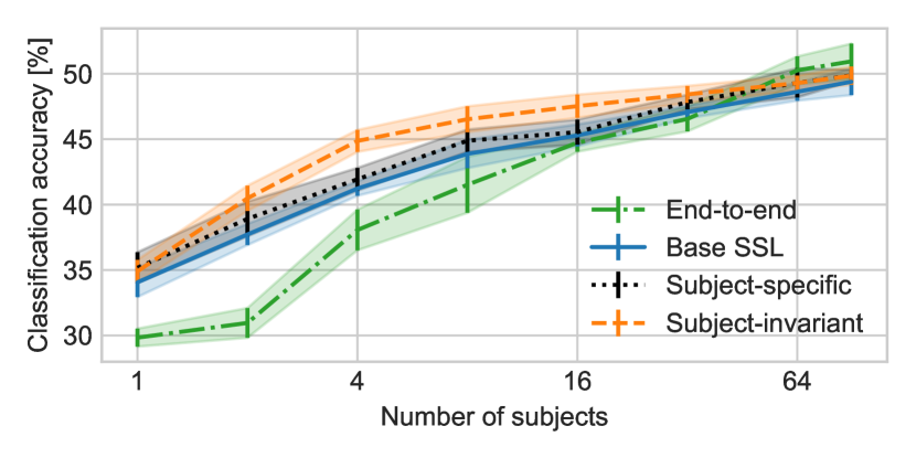
Figure 3: Intersubject testing for 4 classes for the EEG dataset. A linear classifier was trained on top of the frozen encoder using $N$ subjects ($x$-axis) and was tested on 16 unseen subjects. Supervised end-to-end learning was used as a baseline for reference. Fewer subjects were needed for self-supervised models: using labels from 4 subjects for subject-invariant SSL resulted in similar performance to end-to-end learning with 16 subjects.

Fine-Tuning with Supervised Labels.

The models produced from self-supervised learning were evaluated as an initialization for fine-tuning with supervised labels (Table 3). A fully connected layer was attached to the last encoder layer, and this layer along with the entire encoder was fine-tuned (learning rate of 1e-5, batch size of 256, and 200 epochs). For intersubject classification, we achieved 81.6% for 2 classes, and 53.9% for 4 classes. The increased accuracies with using self-supervised-trained models may be attributed to using more data (both action and imagined trials) for training the initial encoder. Reducing subject information in the encoder (lower classification accuracies for subject identification) provided a better initialization for the EEG motor imagery task.

Table 3: EEG classification accuracy [%]. General representations were learned through self-supervised training, and fine-tuning from these models (last three rows) improved accuracies compared to end-to-end (ours) training from random initialization.

	Intersubject		Intrasubject
	2 classa	4 classb	2 classa	4 classb
Kim et al., Random forest [31]	80.1	-	-	-
Dose et al., CNN [32]	80.1	-	-	-
End-to-end (ours)	81.0$\pm$0.9	50.6$\pm$1.0	76.3$\pm$2.4	44.0$\pm$1.6
Fine-tuned from:
Base SSL	81.1$\pm$0.6	52.6$\pm$0.7	78.6$\pm$2.5	50.8$\pm$1.4
Subject-specific	81.6$\pm$0.8	53.9$\pm$0.4	79.3$\pm$2.0	50.5$\pm$1.6
Subject-invariant	81.2$\pm$0.9	52.8$\pm$0.8	79.6$\pm$2.3	49.8$\pm$1.5

^a2 class: right fist and left fist; ^b4 class: right fist, left fist, both fists, and both feet.

4.2 ECG: MIT-BIH Arrhythmia Database

We also evaluated our approach on ECG signals. These signals assist in the detection and characterization of cardiac anomalies on the beat-by-beat level and on the rhythm level. ECG datasets have different challenges for data-driven learning: these datasets are highly imbalanced, and features for detecting anomalies may be tied closely to the subject. We investigated the impact of our methods in these situations. We used the MIT-BIH Arrhythmia Database [28, 33, 34] that is commonly used to benchmark ECG beat and rhythm classification algorithms. This dataset contained 48 ambulatory ECG recordings from 47 different subjects. The 30-min recordings from two sensor leads were digitized to 360 Hz with a bandpass filtering of 0.1–100 Hz. Signals were annotated by expert cardiologists to denote the type of cardiac beat and cardiac rhythms.

Experimental Setup.

The setup described by de Chazal et al. [35] was used. Recordings were divided into a training set and testing set where the different types of beats and rhythms were evenly distributed: 22 recordings in training set, 22 recordings from different subjects in the testing set, and 4 excluded recordings due to paced beats. These 4 excluded recordings were included in the self-supervised learning. Cardiac beats were categorized into 5 classes: normal beat (training / testing samples of 45.8k / 44.2k), supraventricular ectopic beat (SVEB, 0.9k / 1.8k), ventricular ectopic beat (VEB, 3.8k / 3.2k), fusion beat (414 / 388), and unknown beat (8 / 7). The dataset was highly imbalanced, and thus, we followed the common practice of training a 5-class classifier and evaluating its performance in terms of classifying SVEB and VEB. To evaluate different setups, balanced accuracies were computed without the unknown beat due to too few examples for training and testing. The dataset was also labeled with rhythm annotations [36, 37, 38]: normal sinus rhythm (training / testing samples of 3.3k / 2.8k), atrial fibrillation (195 / 541), and other (256 / 362).

For an input window of 704 samples (1.96 sec), a 256-dimensional vector was produced from the encoder $G$ (985k parameters, model details in Appendix). The 256-dimensional vector was used directly to train a linear classifier for beat classification. For rhythm classification, 5 segments (9.78 sec) of data produced 5 vectors that were average pooled into a single vector before applying a linear classifier. Each window of ECG data $x$ was centered by the mode $m(x)$ and normalized by $\mathbb{E}[(x-m(x))^{2}]^{0.5}$. A batch size of 1000 and 260k steps were used for self-supervised training.

Impact of Subject-Aware Training.

Different self-supervised learning setups were used to assess the impact of subject-aware training. Because subject characteristics were closely tied to the beat and rhythm classes, regularization parameter $\lambda$ for subject-invariant training was varied from 0.001 to 1.0. To evaluate the quality of the learned embeddings, a linear classifier was trained on top of the frozen encoder using cross entropy (weight decay of 0.01, learning rate of 1e-3, batch size of 256, and 1k epochs). For rhythm classification, training data had 90% overlap for augmentation; no overlap was used for testing. Examples were randomly sampled with replacement to account for class imbalance.

Similar to EEG, subject-invariant contrastive learning produced the best performing representation for ECG beat and rhythm classification (Table 4). In this case, the subject-invariant regularization $\lambda$ was lowered to 0.1 and 0.01 to maintain sufficient subject information for beat and rhythm classifications. A lower regularization was required due to the uneven distribution of labels between each subject.

Table 4: Linear classifiers to evaluate the information in the frozen encoders. Subject-invariance with minimal subject-based features performed best for classifying beats ($\lambda=$ 0.01) and rhythms (0.001) in terms of overall balanced accuracies.

	Beat			Rhythm		Subject
	Overall	SVEB	VEB	Overall	AFib	ID
	Bal Acc	F1	F1	Bal Acc	F1	Acc
No augmentation	47.9$\pm$3.8	6.9$\pm$2.0	34.1$\pm$3.4	38.0$\pm$1.5	41.5$\pm$4.3	67.5$\pm$1.8
Base SSL	66.3$\pm$6.2	26.7$\pm$8.3	56.1$\pm$8.3	49.4$\pm$3.4	39.7$\pm$6.1	84.7$\pm$0.6
Subject-specific	65.1$\pm$6.1	20.9$\pm$7.7	57.4$\pm$5.9	46.0$\pm$3.7	39.4$\pm$5.3	81.6$\pm$0.8
Subject-invariant
$\lambda=$ 1.0	64.3$\pm$7.9	18.7$\pm$8.5	59.9$\pm$9.2	49.7$\pm$3.3	42.9$\pm$8.4	76.1$\pm$2.2
$\lambda=$ 0.1	68.6$\pm$6.0	26.5$\pm$8.1	62.9$\pm$10.9	51.0$\pm$4.4	44.8$\pm$7.9	79.0$\pm$0.9
$\lambda=$ 0.01	69.8$\pm$5.5	23.9$\pm$8.4	64.1$\pm$8.5	52.3$\pm$5.9	44.6$\pm$5.8	82.9$\pm$0.9
$\lambda=$ 0.001	63.5$\pm$4.4	19.7$\pm$5.3	62.0$\pm$8.0	52.4$\pm$4.3	39.8$\pm$6.1	83.7$\pm$0.9
Random encoder	54.9$\pm$3.8	5.6$\pm$0.9	61.5$\pm$11.3	37.0$\pm$2.0	40.7$\pm$2.8	41.4$\pm$3.5

Abbreviations: SVEB = supraventricular ectopic beat; VEB = ventricular ectopic beat; AFib = atrial fibrillation; ID = subject identification; Bal Acc = balanced accuracy [%]; Acc = accuracy [%]; F1 = F1 score; ID = subject identification (trained with 5 min from all subjects and tested on unseen data of 22 subjects not used for SSL).

Impact of Fewer Labels.

Using the self-supervised model, fewer labels may potentially be needed. The learned encoder was frozen, and a linear classifier was trained on top. To simulate collecting less data, the first N% of contiguous data from each subject was used to train the classifier. This process introduced an uneven increase in labels per class as the percentage of training data was increased as reflected by the varying model performance with respect to the percentage of training data used.

This ECG dataset was in the regime of limited number of subjects and labels which was prone to overfitting as seen in the fully supervised model trained end to end; data augmentation and MixUp [39] were applied for end-to-end training in an attempt to mitigate overfitting. In this scenario, subject-invariant SSL was important in improving performance. For $\lambda$ of 0.1, the performance for subject-invariant SSL was comparable to the base and subject-specific SSL up to 40% of labels and even higher with more labels. By lowering the regularization ($\lambda$ of 0.01) which increased the amount of subject-based features in the learned representations, higher accuracies were achieved.

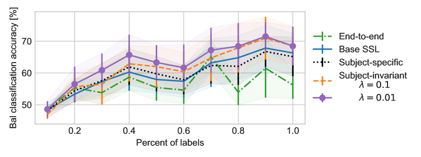
Figure 4: Impact of fewer labels to train a linear classifier on top of the frozen encoders for ECG beat classification. Subject information was needed. By lowering the degree of subject-invariance ($\lambda=$ 0.01), accuracies were improved.

Fine-Tuning with Supervised Labels.

The self-supervised learned models were also evaluated as initializations for fine-tuning with supervised labels. For comparison to previous work [35, 40, 41, 42, 43], weighted cross-entropy was used [44] instead of balanced resampling. We trained an end-to-end supervised model with random initialization as a baseline for comparison. For beat classification, the baseline model achieved an overall accuracy of 91.9%$\pm$1.8%, F1 score for SVEB of 46.7, and F1 score for VEB of 89.2. These results were well within the range of previous work [35, 40, 41, 42, 43] of 89–96% overall accuracies, 23–77 F1 for SVEB, and 63–90 F1 for VEB. Our performance improved by initializing the model with self-supervised learned weights. The best performance was observed when training from the subject-specific SSL encoder with an overall accuracy of 93.2%$\pm$1.6%, F1 score of SVEB of 43.8, and F1 score of VEB of 92.4. The subject-specific training produced a model that can be better fine-tuned for the outlier detection task. See Appendix for more details.

5 Conclusion

This work highlights the importance of subject-awareness for learning biosignal representations. For datasets with a small number of subjects ($<$64 subjects for EEG), the impact of intersubject variability can be reduced. The subject-invariant regularization can be reduced for more subjects or if subject information is important for the downstream task as seen in the analysis with the ECG dataset.

The work presented can be applied to other biosignals, such as signals from the eye (EOG) or muscles (EMG), which are influenced by subject-dependent characteristics. These different data streams are often simultaneously collected, and self-supervised learning with multimodal data will be an area of future work. These unlabeled datasets can become many folds larger than the ones explored, and thus, reducing data requirements and automatically cleaning these datasets will be important extensions.

Our experiments showed that self-supervised learning, specifically contrastive learning, provided a solution to handle biosignals. Moreover, minimal preprocessing was required for these noisy time-series data. With the ease of collecting unlabeled biosignals, extracting meaningful representations will be critical in enabling the application of machine learning for personalization and health.

Broader Impact

Electrophysiological sensors are widely used for monitoring, testing, and diagnosing health conditions. High accuracy and reliability are important when using machine learning for medical applications. We address the lack of labeled data and the biases that labeling may introduce to highly noisy time-series biosignals. However, care must be taken in collecting the unlabeled data to not bias the learning towards a particular data distribution. The use of subject-aware training mitigates this concern, but we still recommend practitioners to check for biases in the learned model. With proper care in data collection and design, the work presented here enables high quality health indicators while improving personalization and promoting privacy through minimization of subject information.

Appendix A EEG: PhysioNet Motor Imagery Dataset [Section 4.1]

Model Architecture.

The models used for processing the raw EEG data are illustrated in Fig. A.2 using the ResNet building blocks shown in Fig. A.1. The input is 320 samples of the 64-channel data which corresponds to 2.0 sec of data (160 Hz sampling rate).

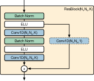
Figure A.1: One-dimensional ResNet [25] building block used for constructing encoder $G$. This block is built using batch normalization [26], exponential linear unit (ELU) activations, and one-dimensional convolutional layers. The convolutional layer is denoted with $Conv1D(N_{i},N_{o},K)$ where $N_{i}$ and $N_{o}$ are the number of input and output channels, respectively. The kernel size is denoted as $K$. The entire ResBlock is denoted as $ResBlock(N_{i},N_{o},K)$. If $N_{i}\neq N_{o}$, a convolutional layer (dashed box) is applied in the skip connection.

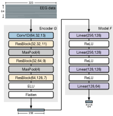
Figure A.2: Models used for EEG processing. Model $G$ encodes raw EEG data into a 256-dimensional vector representation using convolutional layers, ResBlocks (Fig. A.1), max pooling layers ($MaxPool(K)$ corresponds to pooling with a kernel size and stride of $K$), and ELU activation. Model $F$ is used during the self-supervised training stage, and this model is built using fully connected layers represented with $Linear(N_{i},N_{o})$ where $N_{i}$ and $N_{o}$ are the input and output dimensions, respectively.

Supplementary Results for Impact of Transformation.

Detailed results for different parameters for each transformation type are summarized in Table A.1. Because temporal cutout was the most effective augmentation task, variants of this transformation were further investigated. The masked region can be replaced with another signal (mixing) [45], zeros [22], or Gaussian noise. From Fig. A.3, the most effective variant of cutout was replacing the masked region with noise. As noted by Chen et al. [13], stronger augmentations may lead to better learned representation. We hypothesize that the introduction of noise instead of another signal increased the difficulty of learning a representation. Though the masked region was no longer on the data manifold when replaced with noise, this variant of cutout increased noise in the entire model during training by introducing more activated neurons throughout the model.

Table A.1: Impact of different augmentation parameters on representation learning evaluated with a linear classifier trained on top of the learned encoder for the PhysioNet EEG Motor Imagery dataset. Accuracies are computed for the 4-class problem: imagined motion of left fist, right fist, both fists, or feet. These values are computed as mean $\pm$ standard deviation of 10 trials; the best value is bolded in each row if there is a clear maximum. Accuracies are displayed as improvements over baseline of self-supervised learning with no augmentation (36.7%).

Max time delay [samples]	40	80	120	160	200	240	280	320
+Accuracy [%]	6.1	2.4	-2.2	-4.6	-5.9	-6.2	-6.7	-7.3
	$\pm$1.2	$\pm$1.4	$\pm$1.7	$\pm$1.6	$\pm$1.7	$\pm$0.9	$\pm$1.6	$\pm$0.9
Time cutout [samples]	40	80	120	160	200	240	280
+Accuracy [%]	5.5	8.2	9.7	10.5	10.9	3.1	-9.5
	$\pm$1.3	$\pm$0.8	$\pm$0.8	$\pm$1.8	$\pm$2.0	$\pm$4.9	$\pm$2.3
Gaussian noise scale	1.0	2.0	3.0	4.0	5.0	6.0	7.0	8.0	9.0	10.0
+Accuracy [%]	1.3	2.2	2.3	2.9	3.5	3.8	3.3	3.1	3.2	3.7
	$\pm$1.2	$\pm$1.7	$\pm$1.2	$\pm$1.2	$\pm$0.8	$\pm$0.9	$\pm$1.5	$\pm$1.3	$\pm$1.5	$\pm$1.4
Bandstop width [Hz]	1	2	4	8	16	32	64	96
+Accuracy [%]	1.5	1.6	1.7	2.1	2.0	3.0	3.7	2.5
	$\pm$1.4	$\pm$1.3	$\pm$1.4	$\pm$1.0	$\pm$2.9	$\pm$2.0	$\pm$1.5	$\pm$1.5
Signal mixing scale	0.1	0.2	0.3	0.4	0.5	0.6	0.7	0.8	0.9	1.0
+Accuracy [%]	2.4	2.1	2.5	2.6	2.7	2.6	3.1	4.1	5.3	-11.0
	$\pm$1.0	$\pm$0.8	$\pm$1.0	$\pm$1.0	$\pm$0.7	$\pm$0.7	$\pm$1.3	$\pm$1.2	$\pm$1.4	$\pm$0.6
Max spatial shifta	0.02	0.04	0.06	0.08	0.1	0.12	0.14	0.16	0.18
+Accuracy [%]	0.1	-0.3	-0.3	-0.2	-0.1	-0.3	-0.5	-0.0	-0.3
	$\pm$1.1	$\pm$0.6	$\pm$1.4	$\pm$1.1	$\pm$1.0	$\pm$0.7	$\pm$1.0	$\pm$1.1	$\pm$1.3
Max rotation [∘]	10	20	30	40	50	60	70	80	90
+Accuracy [%]	-0.5	-0.1	0.0	-0.3	-1.2	-0.6	-0.2	-0.1	-1.0
	$\pm$1.2	$\pm$0.9	$\pm$0.7	$\pm$1.5	$\pm$1.1	$\pm$1.7	$\pm$0.0	$\pm$0.7	$\pm$1.5
Sensor dropout $p$	0.1	0.2	0.3	0.4	0.5	0.6	0.7	0.8	0.9
+Accuracy [%]	2.8	3.8	3.6	3.2	2.2	0.3	-0.5	-3.2	-3.4
	$\pm$1.3	$\pm$1.5	$\pm$1.4	$\pm$0.9	$\pm$1.0	$\pm$1.5	$\pm$1.2	$\pm$1.4	$\pm$1.6
Sensor cutout radiusa	0.05	0.10	0.15	0.20	0.25	0.30	0.35	0.40	0.45
+Accuracy [%]	1.6	1.5	3.3	3.9	4.1	2.8	1.6	0.1	-0.7
	$\pm$1.1	$\pm$1.4	$\pm$1.0	$\pm$0.9	$\pm$1.4	$\pm$1.3	$\pm$1.2	$\pm$1.5	$\pm$1.5

^aSpatial units are normalized such that the entire extent of the coverage in all directions is between 0 and 1.

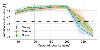
Figure A.3: Variations of augmentation demonstrated for cutout performed on the EEG PhysioNet Motor Imagery dataset. For random cutouts of the time-series signal, the masked region can be replaced with another signal (mixing) [45], zeros (masking) [22], or Gaussian noise. The width of the cutout window is plotted against the accuracy of classifying 4 classes. The data segment is 320 samples wide (2 sec for 160 Hz sampling rate). Baseline of self-supervised training with no augmentation (36.7%) is plotted in the dotted black line.

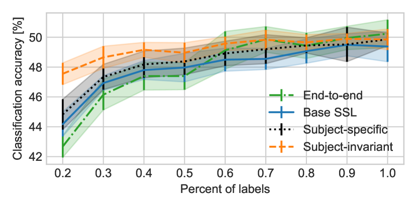
(a) Intersubject testing: train on 90 subjects (also used for self-supervised learning) and test on 16 unseen subjects. The first $N$% of runs ($x$-axis) for each subject were used for training the linear classifier.

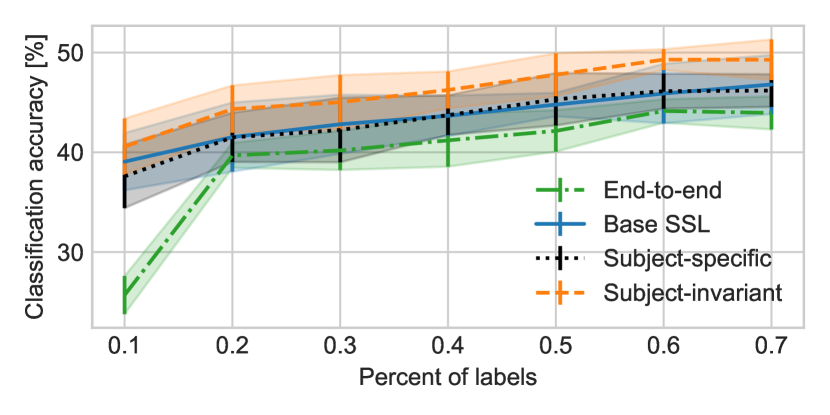
(b) Intrasubject testing: training and testing on 16 subjects that were not used for self-supervised training. The first $N$% of runs ($x$-axis) for each subject were used for training and the last 25% for testing.

Figure A.4: Classification accuracy for 4 classes on the EEG dataset. A linear classifier was trained on top of the frozen encoder. Supervised end-to-end learning was used as a baseline for reference. With limited labels ($<$0.7 for intersubject and any percentage for intrasubject), the subject-invariant consistently out-performed all other approaches due to its ability to limit intersubject variability.

Training Details for Fine-Tuning with Supervised Labels.

The models produced from self-supervised learning were evaluated as an initialization for supervised fine-tuning. More specifically, a randomly-initialized fully connected layer was attached to the end of the encoder, and the fully connected layer and the encoder were updated during the training. Adam optimizer with a learning rate of 1e-5 was used with a batch size of 256 for 200 epochs. For comparison, we also trained a network end-to-end from random initialization with a learning rate of 1e-2, batch size of 1000, and 1k epochs. In all cases, data augmentation and MixUp [39] were used to mitigate overfitting. A representative confusion matrix for the subject-invariant model is shown in Table A.2.

Table A.2: Representative confusion matrix for 4-way classification for EEG decoding using model trained with subject-invariant learning. This model was fine-tuned with supervised labels. The overall accuracy was 54.4%.

		Predicted Label
		Left	Right	Fists	Feet
True label	Left	230	28	67	38
	Right	36	208	48	63
	Fists	69	54	169	66
	Feet	46	54	87	175

Appendix B ECG: MIT-BIH Arrhythmia Database [Section 4.2]

Model Architecture.

The models used for processing the raw ECG data are illustrated in Fig. B.1 using the ResNet building blocks shown in Fig. A.1. The input is 704 samples of the 2-channel data which corresponds to 1.96 sec of data (360 Hz sampling rate).

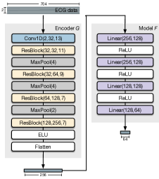
Figure B.1: Models used for ECG processing. Model $G$ encodes raw ECG data into a 256-dimensional vector representation. Model $F$ is used during the self-supervised training stage.

Training Details for Fine-Tuning with Supervised Labels.

The self-supervised learned models were also evaluated as an initialization for supervised training. In literature [35, 40, 41, 42, 43], the accuracies of classifying SVEB and VEB were given higher importance. For comparison, weighted cross-entropy was used [43] instead of balanced resampling. Weights were computed using the following formulation [44]: $w[i]=(1-\beta^{n[i]})/(1-\beta)$ where $n[i]$ is the number of samples for class $i$, and $\beta$ is a hyperparameter set to 0.999. Due to limited number of samples for the unknown beat class ($<$20 in training and test set combined), this class was essentially ignored by assigning the class weight to be the same as the majority class.

One important feature for beat classification is the current RR interval (period of a single heart beat) along with the RR intervals of neighboring heart beats [46, 47]. This feature is unavailable if the receptive field does not cover multiple heart beats as in our setup. The learned representation can be enhanced by including this domain-specific feature. Following previous work [40, 43], the RR intervals before and after the current heart beat were calculated and normalized by the average RR interval over each recording. This RR information was concatenated to the embedding vector produced by the encoder network.

Two fully-connected layers (with 128 dimensions in the hidden layer) were attached to the output of encoder $G$. The encoder $G$ was initialized with the model produced from self-supervised learning. The entire model was then trained end to end during the supervised training. Adam optimizer with a learning rate of 1e-5 was used to update the model with a batch size of 256 for 50 epochs. For comparison, a randomly initialized model was trained end to end with a learning rate of 1e-3, batch size of 256, and 100 epochs. Results are summarized in Table B.1.

The inclusion of the RR interval improved the end-to-end supervised classification performance from F1 score for SVEB of 31.4 to 46.7 and for VEB of 85.8 to 89.2 — well within the range of previous work [35, 40, 41, 42, 43] of 23.2–76.6 for SVEB and 63.4–89.7 for VEB. For beat classification from ECG, we observed the best performance when training from the subject-specific SSL encoder with an overall accuracy of 93.2%$\pm$1.6%, F1 score of SVEB of 43.8, and F1 score of VEB of 92.4. A representative confusion matrix for subject-specific SSL is shown in Table B.2.

Table B.1: Accuracies for intersubject beat classification: the training and testing were performed on separate set of subjects. General representations were learned through self-supervised training, and fine-tuning from these models improved accuracies (last six rows). For conciseness, only the standard deviation of the overall accuracies and F1 scores are reported. Our best results are bolded.

	Overall	SVEB		VEB
	Acc	Acc / Se / +P	F1	Acc / Se / +P	F1
Luo et al. [48]	89.3	96.2 / 15.4 / 47.3	23.2	95.5 / 60.4 / 66.8	63.4
Huang et al. [40]	93.8	95.1 / 91.1 / 42.2	57.7	99.0 / 93.9 / 90.9	92.4
Niu et al. [43]	96.4	- / 76.5 / 76.6	76.6	- / 85.7 / 94.1	89.7
End-to-end (ours)	91.0$\pm$2.0	95.9 / 25.8 / 41.8	31.4$\pm$10.3	97.8 / 95.6 / 78.9	85.8$\pm$8.2
End-to-endR (ours)	91.9$\pm$1.8	96.3 / 44.5 / 52.2	46.7$\pm$14.9	98.4 / 96.4 / 83.4	89.2$\pm$4.3
Fine-tuned from:
Base SSLR	91.7$\pm$1.8	95.6 / 30.2 / 39.2	33.3$\pm$8.1	98.5 / 96.8 / 83.7	89.6$\pm$3.9
Subject-specificR	93.2$\pm$1.6	96.0 / 42.8 / 50.1	43.8$\pm$10.0	98.9 / 96.6 / 88.7	92.4$\pm$3.3
Subject-invariantR
$\lambda=$ 1.0	89.4$\pm$3.0	96.3 / 38.8 / 48.9	42.5$\pm$13.8	97.8 / 95.8 / 77.4	85.4$\pm$4.4
$\lambda=$ 0.1	91.8$\pm$2.2	96.2 / 35.5 / 48.8	40.8$\pm$14.6	98.0 / 95.3 / 79.2	86.3$\pm$5.3
$\lambda=$ 0.01	90.4$\pm$2.2	95.7 / 35.2 / 42.2	37.3$\pm$16.8	98.1 / 96.4 / 80.0	87.2$\pm$5.2
$\lambda=$ 0.001	91.3$\pm$2.7	95.8 / 26.5 / 40.1	31.6$\pm$13.5	98.1 / 96.2 / 80.4	87.2$\pm$7.1

^RIncluding RR-interval information as input to the classifier.
Abbreviations: SVEB = supraventricular ectopic beat; VEB = ventricular ectopic beat; Acc = accuracy [%]; Se = sensitivity [%]; +P = positive predictability; F1 = F1 score.

Table B.2: Representative confusion matrix for beat classification using model trained with subject-specific contrastive learning. This model was fine-tuned with supervised labels. The overall accuracy was 95.1%. F1 scores for SVEB and VEB were 46.1 and 94.6, respectively.

		Predicted Label
		N	SVEB	VEB	F	Q
True label	N	43376	516	115	193	1
	SVEB	1056	717	59	5	0
	VEB	60	39	3067	53	0
	F	299	0	18	71	0
	Q	3	0	4	2	0

Abbreviations: N = normal beat; SVEB = supraventricular ectopic beat; VEB = ventricular ectopic beat; F = fusion beat; Q = unknown beat.

References

- [1] U. R. Acharya, S. Vinitha Sree, G. Swapna, R. J. Martis, and J. S. Suri, “Automated EEG analysis of epilepsy: A review,” Knowledge-Based Systems, vol. 45, pp. 147–165, June 2013.
- [2] F. S. de Aguiar Neto and J. L. G. Rosa, “Depression biomarkers using non-invasive EEG: A review,” Neuroscience & Biobehavioral Reviews, vol. 105, pp. 83–93, Oct. 2019.
- [3] J. Healey and R. Picard, “Detecting stress during real-world driving tasks using physiological sensors,” IEEE Transactions on Intelligent Transportation Systems, vol. 6, pp. 156–166, June 2005.
- [4] I. Misra, C. L. Zitnick, and M. Hebert, “Shuffle and learn: Unsupervised learning using temporal order verification,” in European Conference on Computer Vision, July 2016.
- [5] D. Wei, J. Lim, A. Zisserman, and W. T. Freeman, “Learning and using the arrow of time,” in 2018 IEEE/CVF Conference on Computer Vision and Pattern Recognition, (Salt Lake City, UT), pp. 8052–8060, IEEE, June 2018.
- [6] A. v. d. Oord, Y. Li, and O. Vinyals, “Representation learning with contrastive predictive coding,” arXiv:1807.03748 [cs, stat], Jan. 2019.
- [7] C. Doersch and A. Zisserman, “Multi-task self-supervised visual learning,” in 2017 IEEE International Conference on Computer Vision (ICCV), (Venice), pp. 2070–2079, IEEE, Oct. 2017.
- [8] H. Banville, I. Albuquerque, A. Hyvärinen, G. Moffat, D.-A. Engemann, and A. Gramfort, “Self-supervised representation learning from electroencephalography signals,” in 2019 IEEE 29th International Workshop on Machine Learning for Signal Processing (MLSP), Nov. 2019.
- [9] P. Sarkar and A. Etemad, “Self-supervised learning for ECG-based emotion recognition,” ICASSP 2020 - 2020 IEEE International Conference on Acoustics, Speech and Signal Processing (ICASSP), pp. 3217–3221, May 2020.
- [10] Z. Wu, Y. Xiong, S. Yu, and D. Lin, “Unsupervised feature learning via non-parametric instance-level discrimination,” in Proceedings of the IEEE Conference on Computer Vision and Pattern Recognition, pp. 3733–3742, May 2018.
- [11] P. Sermanet, C. Lynch, Y. Chebotar, J. Hsu, E. Jang, S. Schaal, and S. Levine, “Time-contrastive networks: Self-supervised learning from video,” in 2018 IEEE International Conference on Robotics and Automation (ICRA), pp. 1134–1141, 2018.
- [12] K. He, H. Fan, Y. Wu, S. Xie, and R. Girshick, “Momentum contrast for unsupervised visual representation learning,” arXiv:1911.05722 [cs], Nov. 2019.
- [13] T. Chen, S. Kornblith, M. Norouzi, and G. Hinton, “A simple framework for contrastive learning of visual representations,” arXiv:2002.05709 [cs, stat], Feb. 2020.
- [14] A. Hyvärinen and H. Morioka, “Unsupervised feature extraction by time-contrastive learning and nonlinear ICA,” in Advances in Neural Information Processing Systems 29, 2016.
- [15] E. Tzeng, J. Hoffman, K. Saenko, and T. Darrell, “Adversarial discriminative domain adaptation,” in 2017 IEEE Conference on Computer Vision and Pattern Recognition (CVPR), (Honolulu, HI), pp. 2962–2971, IEEE, July 2017.
- [16] A. Farshchian, J. A. Gallego, L. E. Miller, S. A. Solla, J. P. Cohen, and Y. Bengio, “Adversarial domain adaptation for stable brain-machine interfaces,” International Conference on Learning Representations, 2019.
- [17] E. Tzeng, J. Hoffman, T. Darrell, K. Saenko, and U. Lowell, “Simultaneous deep transfer across domains and tasks,” in The IEEE International Conference on Computer Vision, pp. 4068–4076, 2015.
- [18] Q. Xie, Z. Dai, Y. Du, E. Hovy, and G. Neubig, “Controllable invariance through adversarial feature learning,” in Advances in Neural Information Processing Systems, (Long Beach, CA, USA), 2017.
- [19] O. Ozdenizci, Y. Wang, T. Koike-Akino, and D. Erdogmus, “Learning invariant representations from EEG via adversarial inference,” IEEE Access, vol. 8, pp. 27074–27085, 2020.
- [20] M. Gutmann and A. Hyvarinen, “Noise-contrastive estimation: A new estimation principle for unnormalized statistical models,” in International Conference on Artificial Intelligence and Statistics, (Sardinia, Italy), pp. 297–304, 2010.
- [21] I. Goodfellow, J. Pouget-Abadie, M. Mirza, B. Xu, D. Warde-Farley, S. Ozair, A. Courville, and Y. Bengio, “Generative adversarial nets,” in Advances in Neural Information Processing Systems 27, pp. 2672–2680, 2014.
- [22] T. DeVries and G. W. Taylor, “Improved regularization of convolutional neural networks with cutout,” arXiv:1708.04552 [cs], Nov. 2017.
- [23] M. M. Krell and S. K. Kim, “Rotational data augmentation for electroencephalographic data,” in 2017 39th Annual International Conference of the IEEE Engineering in Medicine and Biology Society (EMBC), pp. 471–474, 2017.
- [24] A. Paszke, S. Gross, F. Massa, A. Lerer, J. Bradbury, G. Chanan, T. Killeen, Z. Lin, N. Gimelshein, L. Antiga, A. Desmaison, A. Kopf, E. Yang, Z. DeVito, M. Raison, A. Tejani, S. Chilamkurthy, B. Steiner, L. Fang, J. Bai, and S. Chintala, “Pytorch: An imperative style, high-performance deep learning library,” in Advances in Neural Information Processing Systems 32, pp. 8026–8037, Curran Associates, Inc., 2019.
- [25] K. He, X. Zhang, S. Ren, and J. Sun, “Identity mappings in deep residual networks,” in European Conference on Computer Vision, pp. 630–645, July 2016.
- [26] S. Ioffe and C. Szegedy, “Batch normalization: Accelerating deep network training by reducing internal covariate shift,” International Conference on Machine Learning, Mar. 2015.
- [27] D. P. Kingma and J. Ba, “Adam: A method for stochastic optimization,” International Conference for Learning Representations, Jan. 2015.
- [28] A. L. Goldberger, L. A. N. Amaral, L. Glass, J. M. Hausdorff, P. C. Ivanov, R. G. Mark, J. E. Mietus, G. B. Moody, C.-K. Peng, and H. E. Stanley, “PhysioBank, PhysioToolkit, and PhysioNet: Components of a new research resource for complex physiologic signals,” Circulation, vol. 101, June 2000.
- [29] G. Schalk, D. McFarland, T. Hinterberger, N. Birbaumer, and J. Wolpaw, “BCI2000: A general-purpose brain-computer interface (BCI) system,” IEEE Transactions on Biomedical Engineering, vol. 51, pp. 1034–1043, June 2004.
- [30] “PhysioNet: EEG motor movement/imagery dataset.” https://physionet.org/content/eegmmidb/1.0.0/, 2009 (last accessed June 2, 2020).
- [31] Y. Kim, J. Ryu, K. K. Kim, C. C. Took, D. P. Mandic, and C. Park, “Motor imagery classification using mu and beta rhythms of EEG with strong uncorrelating transform based complex common spatial patterns,” Computational Intelligence and Neuroscience, vol. 2016, pp. 1–13, 2016.
- [32] H. Dose, J. S. Moller, S. Puthusserypady, and H. K. Iversen, “A deep learning MI - EEG classification model for BCIs,” in 2018 26th European Signal Processing Conference (EUSIPCO), (Rome), pp. 1676–1679, IEEE, Sept. 2018.
- [33] G. Moody and R. Mark, “The impact of the MIT-BIH Arrhythmia Database,” IEEE Engineering in Medicine and Biology Magazine, vol. 20, pp. 45–50, June 2001.
- [34] “PhysioNet: MIT-BIH arrhythmia database.” https://physionet.org/content/mitdb/1.0.0/, 2005 (last accessed June 2, 2020).
- [35] P. de Chazal, M. O’Dwyer, and R. Reilly, “Automatic classification of heartbeats using ECG morphology and heartbeat interval features,” IEEE Transactions on Biomedical Engineering, vol. 51, pp. 1196–1206, July 2004.
- [36] S. Dash, K. H. Chon, S. Lu, and E. A. Raeder, “Automatic real time detection of atrial fibrillation,” Annals of Biomedical Engineering, vol. 37, pp. 1701–1709, Sept. 2009.
- [37] I. H. Bruun, S. M. S. Hissabu, E. S. Poulsen, and S. Puthusserypady, “Automatic atrial fibrillation detection: A novel approach using discrete wavelet transform and heart rate variability,” in 2017 39th Annual International Conference of the IEEE Engineering in Medicine and Biology Society (EMBC), pp. 3981–3984, 2017.
- [38] Z. Wu, X. Feng, and C. Yang, “A deep learning method to detect atrial fibrillation based on continuous wavelet transform,” in 2019 41st Annual International Conference of the IEEE Engineering in Medicine and Biology Society (EMBC), (Berlin, Germany), pp. 1908–1912, IEEE, July 2019.
- [39] H. Zhang, M. Cisse, Y. N. Dauphin, and D. Lopez-Paz, “mixup: Beyond empirical risk minimization,” in International Conference on Learning Representations, Apr. 2018.
- [40] H. Huang, J. Liu, Q. Zhu, R. Wang, and G. Hu, “A new hierarchical method for inter-patient heartbeat classification using random projections and RR intervals,” BioMedical Engineering OnLine, vol. 13, no. 1, p. 90, 2014.
- [41] G. Garcia, G. Moreira, D. Menotti, and E. Luz, “Inter-patient ECG heartbeat classification with temporal VCG optimized by PSO,” Scientific Reports, vol. 7, p. 10543, Dec. 2017.
- [42] S. S. Xu, M.-W. Mak, and C.-C. Cheung, “Towards end-to-end ECG classification with raw signal extraction and deep neural networks,” IEEE Journal of Biomedical and Health Informatics, vol. 23, pp. 1574–1584, July 2019.
- [43] J. Niu, Y. Tang, Z. Sun, and W. Zhang, “Inter-patient ECG classification with symbolic representations and multi-perspective convolutional neural networks,” IEEE Journal of Biomedical and Health Informatics, pp. 1321–1332, 2019.
- [44] Y. Cui, M. Jia, T.-Y. Lin, Y. Song, and S. Belongie, “Class-balanced loss based on effective number of samples,” in 2019 IEEE/CVF Conference on Computer Vision and Pattern Recognition (CVPR), (Long Beach, CA, USA), pp. 9260–9269, IEEE, June 2019.
- [45] S. Yun, D. Han, S. J. Oh, S. Chun, J. Choe, and Y. Yoo, “CutMix: Regularization strategy to train strong classifiers with localizable features,” in International Conference on Computer Vision, pp. 6023–6032, Aug. 2019.
- [46] G. Doquire, G. de Lannoy, D. François, and M. Verleysen, “Feature selection for interpatient supervised heart beat classification,” Computational Intelligence and Neuroscience, vol. 2011, pp. 1–9, 2011.
- [47] C.-C. Lin and C.-M. Yang, “Heartbeat classification using normalized RR intervals and morphological features,” Mathematical Problems in Engineering, vol. 2014, pp. 1–11, 2014.
- [48] K. Luo, J. Li, Z. Wang, and A. Cuschieri, “Patient-specific deep architectural model for ECG classification,” Journal of Healthcare Engineering, vol. 2017, pp. 1–13, 2017.