Fast Transformers with Clustered Attention
Abstract
Transformers have been proven a successful model for a variety of tasks in sequence modeling. However, computing the attention matrix, which is their key component, has quadratic complexity with respect to the sequence length, thus making them prohibitively expensive for large sequences. To address this, we propose clustered attention, which instead of computing the attention for every query, groups queries into clusters and computes attention just for the centroids. To further improve this approximation, we use the computed clusters to identify the keys with the highest attention per query and compute the exact key/query dot products. This results in a model with linear complexity with respect to the sequence length for a fixed number of clusters. We evaluate our approach on two automatic speech recognition datasets and show that our model consistently outperforms vanilla transformers for a given computational budget. Finally, we demonstrate that our model can approximate arbitrarily complex attention distributions with a minimal number of clusters by approximating a pretrained BERT model on GLUE and SQuAD benchmarks with only 25 clusters and no loss in performance.
1 Introduction
Sequence modelling is a fundamental task of machine learning, integral in a variety of applications such as neural machine translation [2], image captioning [31], summarization [18], automatic speech recognition [8] and synthesis [19] etc. Transformers [29] have been proven a powerful tool significantly advancing the state-of-the-art for the majority of the aforementioned tasks. In particular, transformers employ self-attention that allows them to handle long sequences without the vanishing-gradient problem inherent in RNNs [12, 1].
Nonetheless, despite their impressive performance, the use of self-attention comes with computational and memory requirements that scale quadratic to the sequence length, limiting their applicability to long sequences. The quadratic complexity becomes apparent if we consider the core mechanism of self-attention, namely splitting the input sequence into queries and keys and then each query attending to all keys. To this end, recently, there has been an increasing interest for developing methods that address this limitation [7, 28, 5, 13].
These methods can be broadly categorized into two distinct lines of work, those that focus on improving the asymptotic complexity of the self-attention computation [5, 14, 13, 26] and those that aim at developing techniques that make transformers applicable to longer sequences without addressing the quadratic complexity of self-attention [7, 28]. The former limits the amount of keys that each query attends to, thus reducing the asymptotic complexity. The latter increases the length of the sequence that a transformer can attend to without altering the underlying complexity of the self-attention mechanism.
In this work, we propose clustered attention which is a fast approximation of self-attention. Clustered attention makes use of similarities between queries and groups them in order to reduce the computational cost. In particular, we perform fast clustering using locality-sensitive hashing and K-Means and only compute the attention once per cluster. This results in linear complexity for a fixed number of clusters (§ 3.2). In addition, we showcase that we can further improve the quality of our approximation by separately considering the keys with the highest attention per cluster (§ 3.3). Finally, we provide theoretical bounds of our approximation quality with respect to the full attention (§ 3.2.1, § 3.3.1) and show that our model can be applied for inference of pre-trained transformers with minimal loss in performance.
We evaluate our model on two automatic speech recognition datasets and showcase that clustered attention consistently achieves better performance than vanilla attention when the computational budget is equalized. Moreover, we demonstrate that our proposed attention can approximate a pretrained BERT model on the popular GLUE and SQuAD benchmarks with only 25 clusters and without loss in performance.
2 Related Work
In this section, we discuss the most relevant works on scaling transformers to larger sequences. We start by presenting approaches that aim to speed up the attention computation in general. Subsequently, we discuss approaches that speed up transformers without changing the complexity of the attention layer and finally, we summarize the most related works on improving the asymptotic complexity of the attention layer in transformer models.
2.1 Attention Improvements Before Transformers
Attention has been an integral component of neural networks for sequence modelling for several years [2, 31, 4]. However, its quadratic complexity with respect to the sequence length hinders its applicability on large sequences.
Among the first attempts to address this was the work of Britz et al. [3] that propose to aggregate the information of the input sequence into fewer vectors and perform attention with these fewer vectors, thus speeding up the attention computation and reducing the memory requirements. However, the input aggregation is performed using a learned but fixed matrix that remains constant for all sequences, hence significantly limiting the expressivity of the model. Similarly, Chiu & Raffel [6] limit the amount of accessible elements to the attention, by attending monotonically from the past to the future. Namely, if timestep attends to position then timestep cannot attend to any of the earlier positions. Note that in order to speed up the attention computation, the above methods are limiting the number of elements that each layer attends to. Recently, some of these approaches have also been applied in the context of transformers [17].
2.2 Non-asymptotic Improvements
In this section, we summarize techniques that seek to apply transformers to long sequences without focusing on improving the quadratic complexity of self-attention. The most important are Adaptive Attention Span Transformers [28] and Transformer-XL [7].
Sukhbaatar et al. [28] propose to limit the self-attention context to the closest samples (attention span), in terms of relative distance with respect to the time step, thus reducing both the time and memory requirements of self-attention computation. This is achieved using a masking function with learnable parameters that allows the network to increase the attention span if necessary. Transformer-XL [7], on the other hand, seeks to increase the effective sequence length by introducing segment-level recurrent training, namely splitting the input into segments and attending jointly to the previous and the current segment. The above, combined with a new relative positional encoding results in models that attend to more distant positions than the length of the segment used during training.
Although both approaches have been proven effective, the underlying limitations of self-attention still remains. Attending to an element that is timesteps away requires memory and computation. In contrast, our model trades-off a small error in the computation of the full attention for an improved linear asymptotic complexity. This makes processing long sequences possible.
2.3 Improvements in Asymptotic Complexity
Child et al. [5] factorize the self-attention mechanism in local and strided attention. The local attention is computed between the nearest positions and the strided attention is computed between positions that are steps away from each other. When is set to the total asymptotic complexity becomes both in terms of memory and computation time. With the aforementioned factorization, two self-attention layers are required in order for any position to attend to any other position. In addition, the factorization is fixed and data independent. This makes it intuitive for certain signals (e.g. images), however in most cases it is arbitrary. In contrast, our method automatically groups the input queries that are similar without the need for a manually designed factorization. Moreover, in our model, information flows always from every position to every other position.
Set Transformers [14] compute attention between the input sequence , of length and a set of trainable parameters, , called inducing points to get a new sequence , of length . The new sequence is then used to compute the attention with to get the output representation. For a fixed , the asympotic complexity becomes linear with respect to the sequence length. Inducing points are expected to encode some global structure that is task specific. However, this introduces additional model parameters for each attention layer. In contrast to this, we use clustering to project the input to a fixed sequence of smaller length without any increase in the number of parameters. Moreover, we show that not only our method has the same asymptotic complexity, it can also be used to speed up inference of pretrained models without additional training.
Recently, Kitaev et al. [13] introduced Reformer. A method that groups positions based on their similarity using locality-sensitive hashing (LSH) and only computes the attention within groups. For groups of fixed size, the asymptotic complexity of Reformer becomes linear with respect to the sequence length. Note that Reformer constrains the queries and keys of self-attention to be equal. As a result, it cannot be applied to neural machine translation, image captioning or memory networks, or generally any application with heterogenous queries and keys. In addition, as it uses hash collisions to form groups it can only handle a small number of bits, thus significantly reducing the quality of the grouping. Instead, our method uses clustering to group the queries, resulting in significantly better groups compared to hash collisions.
3 Scaling Attention with Fast Clustering
In this section, we formalize the proposed method for approximate softmax attention. In § 3.1, we first discuss the attention mechanism in vanilla transformers and present its computational complexity. We then introduce clustered attention in § 3.2 and show that for queries close in the Euclidean space, the attention difference can be bounded by the distance between the queries. This property allows us to reduce the computational complexity by clustering the queries. Subsequently, in § 3.3 we show that we can further improve the approximation by first extracting the top- keys with the highest attention per cluster and then computing the attention on these keys separately for each query that belongs to the cluster. A graphical illustration of our method is provided in the supplementary material.
3.1 Vanilla Attention
For any sequnce of length , the standard attention mechanism that is used in transformers is the dot product attention introduced by Vaswani et al. [29]. Following standard notation, we define the attention matrix as,
| (1) |
where denotes the queries and denotes the keys. Note that is applied row-wise. Using the attention weights and the values , we compute the new values as follows,
| (2) |
An intuitive understanding of the attention, as described above, is that given we create new values as the weighted average of the old ones, where the weights are defined by the attention matrix . Computing equation 1 requires operations and the weighted average of equation 2 requires . This results in an asymptotic complexity of .
3.2 Clustered Attention
Instead of computing the attention matrix for all queries, we group them into clusters and compute the attention only for these clusters. Then, we use the same attention weights for queries that belong to the same cluster. As a result, the attention computation now becomes , where .
More formally, let us define , a partitioning of the queries into non-overlapping clusters, such that, , if the -th query belongs to the -th cluster and otherwise. Using this partitioning, we can now compute the clustered attention. First, we compute the cluster centroids as follows,
| (3) |
where is the centroid of the -th cluster. Let us denote as the centroid matrix. Now, we can compute the clustered attention as if were the queries. Namely, we compute the clustered attention matrix
| (4) |
and the new values
| (5) |
Finally, the value of the -th query becomes the value of its closest centroid, namely,
| (6) |
From the above analysis, it is evident that we only need to compute the attention weights and the weighted average of the values once per cluster. Then, we can broadcast the same value to all queries belonging to the same cluster. This allows us to reduce the number of dot products from for each query to for each cluster, which results in an asymptotic complexity of .
Note that in practice, we use multi-head attention, this means that two queries belonging to the same cluster can be clustered differently in another attention head. Moreover, the output of the attention layer involves residual connections. This can cause two queries belonging to the same cluster to have different output representations. The combined effect of residual connections and multi-head attention allows new clustering patterns to emerge in subsequent layers.
3.2.1 Quality of the approximation
From the above, we show that grouping queries into clusters can speed-up the self-attention computation. However, in the previous analysis, we do not consider the effects of clustering on the attention weights . To address this, we derive a bound for the approximation error. In particular, we show that the difference in attention can be bounded as a function of the Euclidean distance between the queries.
Proposition 1.
Given two queries and such that ,
| (7) |
where denotes the spectral norm of .
Proof.
Proposition 1 shows that queries that are close in Euclidean space have similar attention distributions. As a result, the error in the attention approximation for the -th query assigned to the -th cluster can be bounded by its distance from the cluster centroid .
3.2.2 Grouping the Queries
From the discussion, we have shown that given a representative set of queries, we can approximate the attention with fewer computations. Thus, now the problem becomes finding this representative set of queries. K-Means clustering minimizes the sum of squared distances between the cluster members, which would be optimal given our analysis from § 3.2.1. However, for a sequence of length one iteration of Lloyd’s algorithm for the K-Means optimization problem has an asymptotic complexity . To speed up the distance computations, we propose to use Locality-Sensitive Hashing (LSH) on the queries and then K-Means in Hamming space. In particular, we use the sign of random projections [27] to hash the queries followed by K-Means clustering with hamming distance as the metric. This results in an asymptotic complexity of , where is the number of Lloyd iterations and is the number of bits used for hashing.
3.3 Improving clustered attention
In the previous section, we show that clustered attention provides a fast approximation for softmax attention. In this section, we discuss how this approximation can be further improved by considering separately the keys with the highest attention. To intuitively understand the importance of the above, it suffices to consider a scenario where a key with low attention for some query gets a high attention as approximated with the cluster centroid. This can happen when the number of clusters are too low or due to the convergence failure of K-Means. For the clustered attention, described in § 3.2, this introduces significant error in the computed value. The variation discussed below addresses such limitations.
After having computed the clustered attention from equation 4, we find the keys with the highest attention for each cluster. The main idea then is to improve the attention approximation on these top- keys for each query that belongs to the cluster. To do so, we first compute the dot product attention as defined in equation 1 on these top- keys for all queries belonging to this cluster. For any query, the computed attention on these top- keys will sum up to one. This means that it cannot be directly used to substitute the clustered-attention on these keys. To address this, before substition, we scale the computed attention by the total probability mass assigned by the clustered attention to these top- keys.
More formally, we start by introducing , where if the -th key is among the top- keys for the -th cluster and 0 otherwise. We can then compute the probability mass, let it be , of the top- keys for the -th cluster, as follows
| (9) |
Now we formulate an improved attention matrix approximation as follows
| (10) |
Note that in the above, denotes the -th query belonging to the -th cluster and is ommited for clarity. In particular, equation 10 selects the clustered attention of equation 4 for keys that are not among the top- keys for a given cluster. For the rest, it redistributes the mass according to the dot product attention of the queries with the top- keys. The corresponding new values, , are a simple matrix product of with the values,
| (11) |
Equation 11 can be decomposed into clustered attention computation and two sparse dot products, one for every query with the top- keys and one for the top- attention weights with the corresponding values. This adds to the asymptotic complexity of the attention approximation of equation 4.
3.3.1 Quality of the approximation
In the following, we provide proof that improved clustered attention (eq. 10) is a direct improvement over the clustered attention (eq. 4), in terms of the distance from the attention matrix .
Proposition 2.
For the -th query belonging to the -th cluster, the improved clustered attention and clustered attention relate to the full attention as follows,
| (12) |
Due to lack of space, the proof of the above proposition is presented in the supplementary material. From equation 12 it becomes evident that improved clustered attention will always approximate the full attention better compared to clustered attention.
4 Experiments
In this section, we analyze experimentally the performance of our proposed method. Initially, we show that our model outperforms our baselines for a given computational budget on a real-world sequence to sequence task, namely automatic speech recognition on two datasets, the Wall Street Journal dataset (§ 4.1) and the Switchboard dataset (§ 4.2). Subsequently, in § 4.3, we demonstrate that our model can approximate a pretrained BERT model [16] on the GLUE [30] and SQuAD [25] benchmarks with minimal loss in performance even when the number of clusters is less than one tenth of the sequence length. Due to lack of space, we also provide, in the supplementary material, a thorough benchmark that showcases the linear complexity of clustered attention and an ablation study regarding how the number of clusters scales with respect to the sequence length.
We compare our model with the vanilla transformers [29], which we refer to as full and the Reformer [13], which we refer to as lsh-X, where denotes the rounds of hashing. We refer to clustered attention, introduced in § 3.2, as clustered-X and to improved clustered attention, introduced in § 3.3, as i-clustered-X, where denotes the number of clusters. Unless mentioned otherwise we use for the top- keys with improved clustered.
All experiments are conducted using NVidia GTX 1080 Ti with GB of memory and all models are implemented in PyTorch [20]. For Reformer we use a PyTorch port of the published code. Note that we do not use reversible layers since it is a technique that could be applied to all methods. Our PyTorch code can be found at https://clustered-transformers.github.io.
4.1 Evaluation on Wall Street Journal (WSJ)
In our first experiment, we employ the Wall-Street Journal dataset [21]. The input to all transformers is -dimensional filter-bank features with fixed positional embeddings. We train using Connectionist Temporal Classification (CTC) [11] loss with phonemes as ground-truth labels. The approximate average and maximum sequence lengths for the training inputs are and respectively.
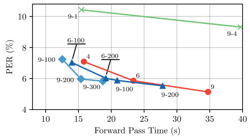
Speed Accuracy Trade-off: We start by comparing the performance of our proposed model with various transformer variants under an equalized computational budget. To this end, we train full with , and layers to get a range of the required computation time and achieved phone error rate (PER). Similarly, we train i-clustered with and layers. Both models are trained with and clusters. We also train clustered with layers, and , and clusters. Finally, we train Reformer with layers, and and hashing rounds. We refer the reader to our supplementary for the specifics of all transformer architectures as well as their training details. In figure 1(a), we plot the achieved PER on the validation set with respect to the required time to perform a full forward pass. Our i-clustered achieves lower PER than all other baselines for a given computational budget.
Approximation Quality: To assess the approximation capabilities of our method, we train different transformer variants on the aforementioned task and evaluate them using other self-attention implementations during inference. As the Reformer requires the queries to be identical to the keys to evaluate its approximation ability we also train a full attention model with shared queries and keys, which we refer to as shared-full. Note that both clustered attention and improved clustered attention can be used for approximating shared-full, simply by setting keys to be equal to queries. Table 1 summarizes the results. We observe that improved clustered attention (7-8 rows) achieves the lowest phone error rate in every comparison. This implies that it is the best choice for approximating pre-trained models. In addition, we also note that as the number of clusters increases, the approximation improves as well.
| Train with | |||||||
|---|---|---|---|---|---|---|---|
| full | shared-full | lsh-1 | lsh-4 | clustered-100 | i-clustered-100 | ||
| Evaluate with | full | 5.14 | - | - | - | 7.10 | 5.56 |
| shared-full | - | 6.57 | 25.16 | 41.61 | - | - | |
| lsh-1 | - | 71.40 | 10.43 | 13.76 | - | - | |
| lsh-4 | - | 64.29 | 9.35 | 9.33 | - | - | |
| clustered-100 | 44.88 | 40.86 | 68.06 | 66.43 | 7.06 | 18.83 | |
| clustered-200 | 21.76 | 25.86 | 57.75 | 57.24 | 6.34 | 8.95 | |
| i-clustered-100 | 9.29 | 13.22 | 41.65 | 48.20 | 8.80 | 5.95 | |
| i-clustered-200 | 6.38 | 8.43 | 30.09 | 42.43 | 7.71 | 5.60 | |
| oracle-top | 17.16 | 77.18 | 43.35 | 59.38 | 24.32 | 6.96 | |
Furthermore, to show that the top keys alone are not sufficient for approximating full, we also compare with an attention variant, that for each query only keeps the keys with the highest attention. We refer to the latter as oracle-top. We observe that oracle-top achieves significantly larger phone error rate than improved clustered in all cases. This implies that improved clustered attention also captures the significant long tail of the attention distribution.
Convergence Behaviour: In Table 2, we report the required time per epoch as well as the total training time for all transformer variants with 9 layers. For completeness, we also provide the corresponding phone error rates on the test set. We observe that clustered attention is more than two times faster than full (per epoch) and achieves significantly lower PER than both Reformer variants (lsh- and lsh-). Improved clustered is the only method that is not only faster per epoch but also in total wall-clock time required to converge.
| full | lsh-1 | lsh-4 | clustered-100 | i-clustered-100 | |
| PER (%) | 5.03 | 9.43 | 8.59 | 7.50 | 5.61 |
| Time/Epoch (s) | 2514 | 1004 | 2320 | 803 | 1325 |
| Convergence Time (h) | 87.99 | 189.64 | 210.09 | 102.15 | 72.14 |
4.2 Evaluation on Switchboard
We also evaluate our model on the Switchboard dataset [10], which is a collection of telephone conversations on common topics among strangers. All transformers are trained with lattice-free MMI loss [24] and as inputs we use -dimensional filter-bank features with fixed positional embeddings. The average input sequence length is roughly and the maximum sequence length is approximately . Details regarding the transformer architectures as well as their training details are provided in the supplementary.
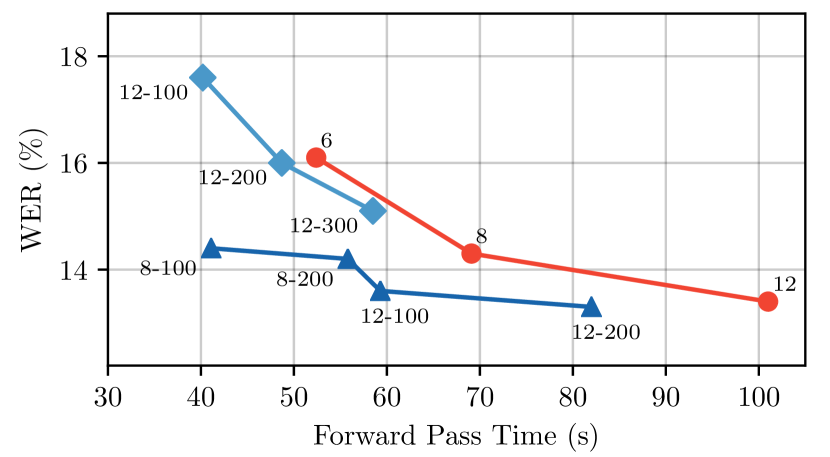
Speed Accuracy Trade-off: Similar to § 4.1, we compare the performance of various transformer models given a specific computational budget. To this end, we train full with and layers. Similarly, we train i-clustered with and layers; both with and clusters. Finally, we also train clustered with layers, and and clusters. In figure 1(b), we plot the achieved word error rate (WER) in the validation set of Switchboard with respect to the required time to perform a full forward pass. Our i-clustered is consistently better than full for a given computational budget. In particular, for a budget of approximately seconds, improved clustered achieves more than percentage points lower WER. Furthermore, we note that it is consistently better than clustered attention for all computational budgets.
Convergence Behaviour: Table 3 summarizes the computational cost of training the transformer models with 12 layers in the Switchboard dataset as well as the WER in the test set. We observe that due to the larger sequences in this dataset both clustered and i-clustered are faster to train per epoch and with respect to total required wall-clock time.
| full | clustered-100 | i-clustered-100 | |
|---|---|---|---|
| WER (%) | 15.0 | 18.5 | 15.5 |
| Time/Epoch (h) | 3.84 | 1.91 | 2.57 |
| Convergence Time (h) | 228.05 | 132.13 | 127.44 |
4.3 RoBERTa Approximation
To highlight the ability of our model to approximate arbitrarily complicated attention distributions, we evaluate our proposed method on the approximation of a fine-tuned RoBERTa model [16] on the GLUE [30] and SQuAD [25] benchmarks. In particular, we evaluate on different tasks, among which there are tasks such as question answering (SQuAD) and textual entailment (RTE), which exhibit arbitrary and sparse attention patterns. We refer the reader to Wang et al. [30], Rajpurkar et al. [25] for a detailed analysis of all tasks.
For the GLUE tasks, the maximum sequence length is 128 while for SQuAD, it is 384. For each task, we use clusters for approximation which is less than and of the input sequence length for GLUE and SQuAD tasks respectively. In Table 4, we summarize the performance per task. We observe that improved clustered performs as well as the full transformer in all tasks but SQuAD, in which it is only marginally worse. Moreover, we note that clustered performs significantly worse in tasks that require more complicated attention patterns such as SQuAD and RTE. For inference time, full was faster than the clustered attention variants due to short sequence lengths.
| CoLA | MNLI | MRPC | QNLI | QQP | RTE | SST-2 | STS-B | WNLI | SQuAD | |
|---|---|---|---|---|---|---|---|---|---|---|
| full | 0.601 | 0.880 | 0.868 | 0.929 | 0.915 | 0.682 | 0.947 | 0.900 | 0.437 | 0.904 |
| clustered-25 | 0.598 | 0.794 | 0.436 | 0.746 | 0.894 | 0.498 | 0.944 | 0.789 | 0.437 | 0.006 |
| i-clustered-25 | 0.601 | 0.880 | 0.873 | 0.930 | 0.915 | 0.704 | 0.947 | 0.900 | 0.437 | 0.876 |
5 Conclusions
We have presented clustered attention a method that approximates vanilla transformers with significantly lower computational requirements. In particular, we have shown that our model can be up to faster during training and inference with minimal loss in performance. In contrast to recent fast variations of transformers, we have also shown that our method can efficiently approximate pre-trained models with full attention while retaining the linear asymptotic complexity.
The proposed method opens several research directions towards applying transformers on long sequence tasks such as music generation, scene flow estimation etc. We consider masked language modeling for long texts to be of particular importance, as it will allow finetuning for downstream tasks that need a context longer than the commonly used 512 tokens.
Broader Impact
This work contributes towards the wider adoption of transformers by reducing their computational requirements; thus enabling their use on embedded or otherwise resource constrained devices. In addition, we have shown that for long sequences clustered attention can result to almost reduction in GPU training time which translates to equal reduction in CO2 emmisions and energy consumption.
Acknowledgements
Apoorv Vyas was supported by the Swiss National Science Foundation under grant number FNS-30213 ”SHISSM”. Angelos Katharopoulos was supported by the Swiss National Science Foundation under grant numbers FNS-30209 ”ISUL” and FNS-30224 ”CORTI”.
References
- Arjovsky et al. [2016] Arjovsky, M., Shah, A., and Bengio, Y. Unitary evolution recurrent neural networks. In International Conference on Machine Learning, pp. 1120–1128, 2016.
- Bahdanau et al. [2014] Bahdanau, D., Cho, K., and Bengio, Y. Neural machine translation by jointly learning to align and translate. arXiv preprint arXiv:1409.0473, 2014.
- Britz et al. [2017] Britz, D., Guan, M. Y., and Luong, M.-T. Efficient attention using a fixed-size memory representation. arXiv preprint arXiv:1707.00110, 2017.
- Chan et al. [2016] Chan, W., Jaitly, N., Le, Q., and Vinyals, O. Listen, attend and spell: A neural network for large vocabulary conversational speech recognition. In 2016 IEEE International Conference on Acoustics, Speech and Signal Processing (ICASSP), pp. 4960–4964. IEEE, 2016.
- Child et al. [2019] Child, R., Gray, S., Radford, A., and Sutskever, I. Generating long sequences with sparse transformers. arXiv preprint arXiv:1904.10509, 2019.
- Chiu & Raffel [2017] Chiu, C.-C. and Raffel, C. Monotonic chunkwise attention. arXiv preprint arXiv:1712.05382, 2017.
- Dai et al. [2019] Dai, Z., Yang, Z., Yang, Y., Cohen, W. W., Carbonell, J., Le, Q. V., and Salakhutdinov, R. Transformer-xl: Attentive language models beyond a fixed-length context. arXiv preprint arXiv:1901.02860, 2019.
- Dong et al. [2018] Dong, L., Xu, S., and Xu, B. Speech-transformer: a no-recurrence sequence-to-sequence model for speech recognition. In 2018 IEEE International Conference on Acoustics, Speech and Signal Processing (ICASSP), pp. 5884–5888. IEEE, 2018.
- Gao & Pavel [2017] Gao, B. and Pavel, L. On the properties of the softmax function with application in game theory and reinforcement learning, 2017.
- Godfrey et al. [1992] Godfrey, J. J., Holliman, E. C., and McDaniel, J. Switchboard: Telephone speech corpus for research and development. In [Proceedings] ICASSP-92: 1992 IEEE International Conference on Acoustics, Speech, and Signal Processing, volume 1, pp. 517–520. IEEE, 1992.
- Graves et al. [2006] Graves, A., Fernández, S., Gomez, F., and Schmidhuber, J. Connectionist temporal classification: Labelling unsegmented sequence data with recurrent neural networks. In Proceedings of the 23rd International Conference on Machine Learning, 2006.
- Hochreiter et al. [2001] Hochreiter, S., Bengio, Y., Frasconi, P., and Schmidhuber, J. Gradient flow in recurrent nets: the difficulty of learning long-term dependencies, 2001.
- Kitaev et al. [2020] Kitaev, N., Kaiser, L., and Levskaya, A. Reformer: The efficient transformer. In International Conference on Learning Representations, 2020. URL https://openreview.net/forum?id=rkgNKkHtvB.
- Lee et al. [2019] Lee, J., Lee, Y., Kim, J., Kosiorek, A., Choi, S., and Teh, Y. W. Set transformer: A framework for attention-based permutation-invariant neural networks. In International Conference on Machine Learning, 2019.
- Liu et al. [2020] Liu, L., Jiang, H., He, P., Chen, W., Liu, X., Gao, J., and Han, J. On the variance of the adaptive learning rate and beyond. In International Conference on Learning Representations, 2020. URL https://openreview.net/forum?id=rkgz2aEKDr.
- Liu et al. [2019] Liu, Y., Ott, M., Goyal, N., Du, J., Joshi, M., Chen, D., Levy, O., Lewis, M., Zettlemoyer, L., and Stoyanov, V. Roberta: A robustly optimized bert pretraining approach. arXiv preprint arXiv:1907.11692, 2019.
- Ma et al. [2020] Ma, X., Pino, J. M., Cross, J., Puzon, L., and Gu, J. Monotonic multihead attention. In International Conference on Learning Representations, 2020. URL https://openreview.net/forum?id=Hyg96gBKPS.
- Maybury [1999] Maybury, M. Advances in automatic text summarization. MIT press, 1999.
- Oord et al. [2016] Oord, A. v. d., Dieleman, S., Zen, H., Simonyan, K., Vinyals, O., Graves, A., Kalchbrenner, N., Senior, A., and Kavukcuoglu, K. Wavenet: A generative model for raw audio. arXiv preprint arXiv:1609.03499, 2016.
- Paszke et al. [2019] Paszke, A., Gross, S., Massa, F., Lerer, A., Bradbury, J., Chanan, G., Killeen, T., Lin, Z., Gimelshein, N., Antiga, L., et al. Pytorch: An imperative style, high-performance deep learning library. In Advances in Neural Information Processing Systems, pp. 8024–8035, 2019.
- Paul & Baker [1992] Paul, D. B. and Baker, J. M. The design for the wall street journal-based csr corpus. In Proceedings of the Workshop on Speech and Natural Language, HLT ’91, 1992.
- Povey et al. [2011] Povey, D., Ghoshal, A., Boulianne, G., Burget, L., Glembek, O., Goel, N., Hannemann, M., Motlicek, P., Qian, Y., Schwarz, P., Silovsky, J., Stemmer, G., and Vesely, K. The kaldi speech recognition toolkit. In IEEE Workshop on Automatic Speech Recognition and Understanding. IEEE Signal Processing Society, 2011.
- Povey et al. [2015] Povey, D., Zhang, X., and Khudanpur, S. Parallel training of dnns with natural gradient and parameter averaging. In In International Conference on Learning Representations: Workshop track, 2015.
- Povey et al. [2016] Povey, D., Peddinti, V., Galvez, D., Ghahremani, P., Manohar, V., Na, X., Wang, Y., and Khudanpur, S. Purely sequence-trained neural networks for asr based on lattice-free mmi. In Interspeech, pp. 2751–2755, 2016.
- Rajpurkar et al. [2018] Rajpurkar, P., Jia, R., and Liang, P. Know what you don’t know: Unanswerable questions for squad. In Proceedings of the 56th Annual Meeting of the Association for Computational Linguistics (Volume 2: Short Papers), pp. 784–789, 2018.
- Roy et al. [2020] Roy, A., Saffar, M., Vaswani, A., and Grangier, D. Efficient content-based sparse attention with routing transformers. arXiv preprint arXiv:1908.03265, 2020.
- Shrivastava & Li [2014] Shrivastava, A. and Li, P. Asymmetric lsh (alsh) for sublinear time maximum inner product search (mips). In Advances in Neural Information Processing Systems, pp. 2321–2329, 2014.
- Sukhbaatar et al. [2019] Sukhbaatar, S., Grave, E., Bojanowski, P., and Joulin, A. Adaptive attention span in transformers. arXiv preprint arXiv:1905.07799, 2019.
- Vaswani et al. [2017] Vaswani, A., Shazeer, N., Parmar, N., Uszkoreit, J., Jones, L., Gomez, A. N., Kaiser, Ł., and Polosukhin, I. Attention is all you need. In Advances in neural information processing systems, pp. 5998–6008, 2017.
- Wang et al. [2019] Wang, A., Singh, A., Michael, J., Hill, F., Levy, O., and Bowman, S. R. GLUE: A multi-task benchmark and analysis platform for natural language understanding. In 7th International Conference on Learning Representations, ICLR 2019, New Orleans, LA, USA, May 6-9, 2019, 2019.
- Xu et al. [2015] Xu, K., Ba, J., Kiros, R., Cho, K., Courville, A., Salakhudinov, R., Zemel, R., and Bengio, Y. Show, attend and tell: Neural image caption generation with visual attention. In International conference on machine learning, pp. 2048–2057, 2015.
Supplementary Material for
Fast Transformers with Clustered Attention
Appendix A Scaling Attention with Fast Clustering
In this section we present graphical illustrations for the proposed clustered and i-clustered attention models in § A.1 and § A.2 respectively.
A.1 Clustered attention
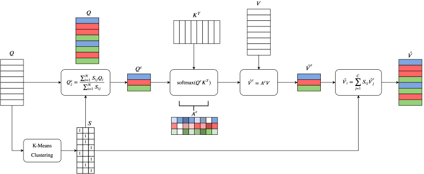
In figure 2, we present the steps involved in clustered attention computation for an example sequence with queries and the number of clusters set to . We first cluster the queries using the K-means clustering to output which indicates the membership of queries to different clusters. We use different colors to represent different clusters. After clustering, the centroids are used to compute the attention weights and the new values for the centroids. Finally, the values are broadcasted to get the new values corresponding to each query.
A.2 Improved clustered attention
In this section, we first describe how we can efficiently compute the i-clustered attention using sparse dot products with the top- keys and values. We then present the flow chart demonstrating the same.
As discussed in the § 3.3 of the main paper, the improved attention matrix approximation for the query, belonging to the cluster is computed as follows:
| (13) |
where, , stores the top- keys for each cluster. if the -th key is among the top- keys for the -th cluster and 0 otherwise.
As described in the main paper, is the total probability mass on the top- keys for the -th cluster given by:
| (14) |
Note that we can compute the attention weights on the top- keys by first taking sparse dot-product of with the top- keys followed by the softmax activation and rescaling with total probablity mass . For the rest of the keys, the attention weight is the clustered-attention weight .
Similarly, the new values can be decomposed into the following two terms,
| (15) |
where is weighted average of the values corresponding to the top- keys with weights being the improved attention on the top- keys. is the weighted average of the rest of the values with weights being the clustered attention . The following equations show how we compute and ,
| (16) |
| (17) |
Note that is weighted average of values for each query and thus requires operations. only needs to be computed once per-cluster centroid and thus requires operations.
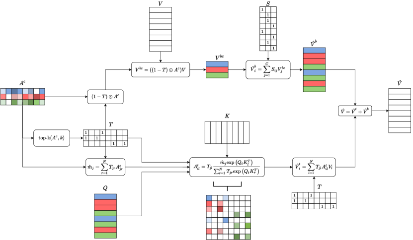
In figure 3 we present the i-clustered attention computation for the same example sequence with queries and the number of clusters and top- keys set to 3. The lower half of the figure shows the new value computed by first taking sparse dot-products with the top 3 keys to get the attention weights. This is followed by taking the weighted average of the 3 correponding values. The top half of the figure shows the computation. This is same as clustered attention computation but with attention weights corresponding to top keys set to for . The resulting values is the sum of and .
Appendix B Quality of the approximation
Proposition 3.
For the -th query belonging to the -th cluster, the improved clustered attention and clustered attention relate to the full attention as follows,
| (18) |
Proof.
As discussed before, the improved attention matrix approximation for the query, is computed as follows:
| (19) |
where, , stores the top- keys for each cluster, if the -th key is among the top- keys for the -th cluster and 0 otherwise. is the total probability mass on the top- keys for the -th cluster, computed as follows:
| (20) |
Given the full attention , equation 19 can be simplified to
| (21) |
where, is the total probability mass on the same top- keys for the -th query, computed using the true attention , as follows:
| (22) | ||||
| (23) |
Without loss of generality, let us assume, and .
In this case, equation 21 can be written as:
| (24) |
The total probability masses on the top- keys, and can now be expressed as:
| (25) | ||||
| (26) |
From equation 24 it is clear that the clustered attention, , and the improved clustered attention, , only differ on the keys . Thus, it suffices to show that has lower approximation error on these keys. The approximation error on the top- keys , let it be , between the i-clustered attention and the full attention is as follows:
| (27) | ||||
| (28) | ||||
| (29) | ||||
| (30) | ||||
| (31) | ||||
| (32) | ||||
| (33) | ||||
| (34) |
Therefore,
| (35) | ||||
| (36) | ||||
| (37) | ||||
| (38) |
∎
Appendix C Experiments
C.1 Time and Memory Benchmark
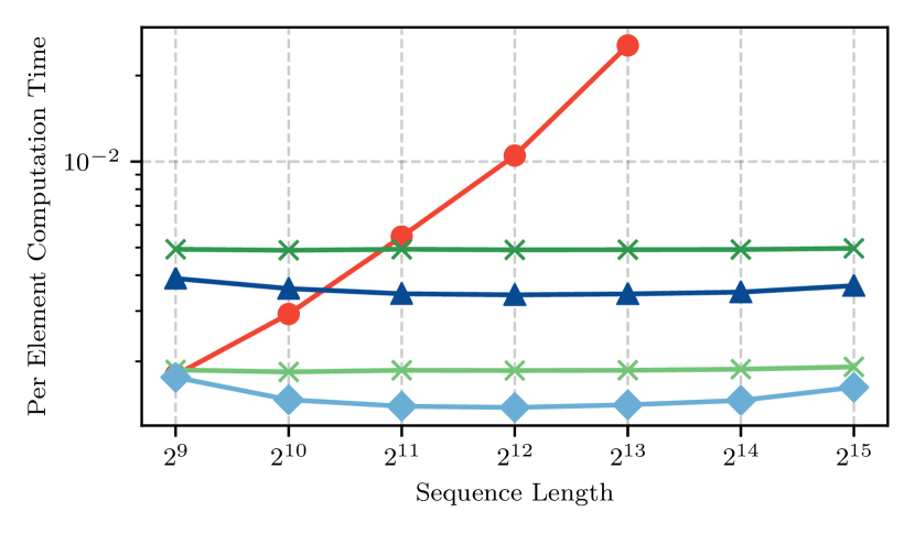
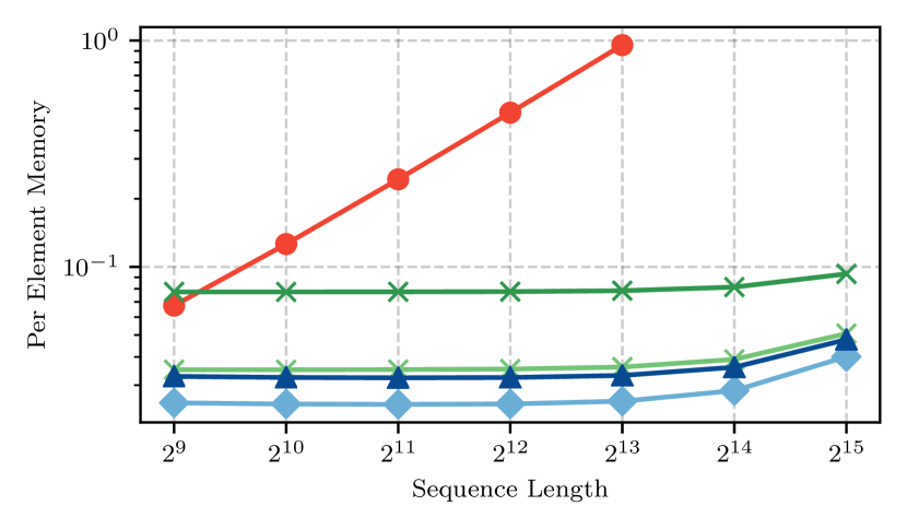
To measure the computational cost, we compare the memory consumption and computation time on artificially generated sequences of various lengths. For clustered attention we use clusters, bits for the LSH, and Lloyd iterations for the K-Means. For the improved clustered attention, we use the same configuration with . For Reformer, we evaluate on two variants using and rounds of hashing. All models consist of layer with attention heads, embedding dimension of for each head, and a feed-forward dimension of .
In this experiment, we measure the required memory and GPU time per single sequence element to perform a forward/backward pass for the various self-attention models. Figure 4 illustrates how these metrics evolve as the sequence length increases from to . For a fair comparison, we use the maximum possible batch size for each method and we divide the computational cost and memory with the number of samples in each batch and the sequence length.
We note that, in contrast to all other methods, vanilla transformer scales quadratically with respect to the sequence length and does not fit in GPU memory for sequences longer than elements. All other methods scale linearly. Clustered attention becomes faster than the vanilla transformer for sequences with elements or more, while improved clustered attention surpasses it for sequences with elements. Note that with respect to per sample memory, both clustered and improved clustered attention perform better than all other methods. This can be explained by the fact that our method does not require storing intermediate results to compute the gradients from multiple hashing rounds as Reformer does. It can be seen, that lsh- is faster than the improved clustered clustered attention, however, as also mentioned by [13] Reformer requires multiple hashing rounds to generalize.
C.2 Ablation on clusters and sequence length
Accuracy with respect to clusters and hashing rounds

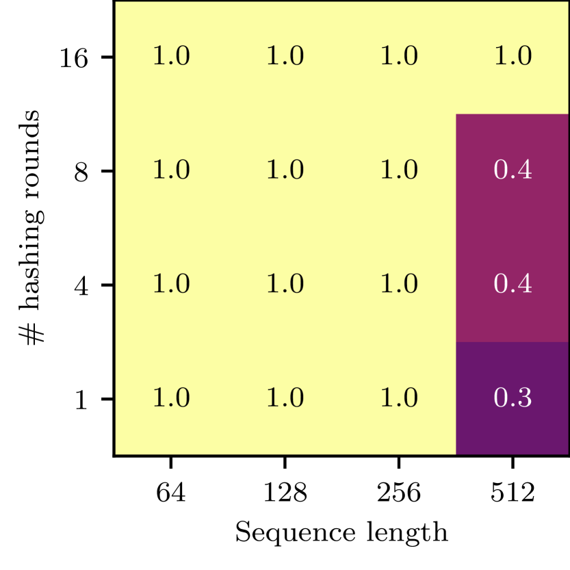
Following [13], we introduce a synthetic task to analyze the relationship between the number of clusters and sequence length. In our task, the transformer models need to copy some symbols that are masked out from either the first or second half of the sequence. In particular, we generate a random sequence of tokens and we prepend a unique separator token, let it be . The sequence is then copied to get a target of the form , where , is the number of possible symbols and is the sequence length. To generate the input, we replace some symbols from the first half of the sequence and some different symbols from the second half, such that the target sequence can be reconstructed from the input. An example of an input output pair with can be seen in figure 6. Note that to solve this task, transformers simply need to learn to attend to the corresponding tokens in the two identical halves of the sequence.
| Input | 0 | 4 | M | 2 | 2 | 0 | 4 | 5 | M | 2 |
|---|---|---|---|---|---|---|---|---|---|---|
| Output | 0 | 4 | 5 | 2 | 2 | 0 | 4 | 5 | 2 | 2 |
We set the sequence length to one of which means the input length varies between and . For each sequence, we sample tokens uniformly from and randomly mask out of the tokens. To analyze the impact of number of clusters on performance, we train full transformer as well as clustered variants with different number of clusters and Reformer with different number of hashing rounds.
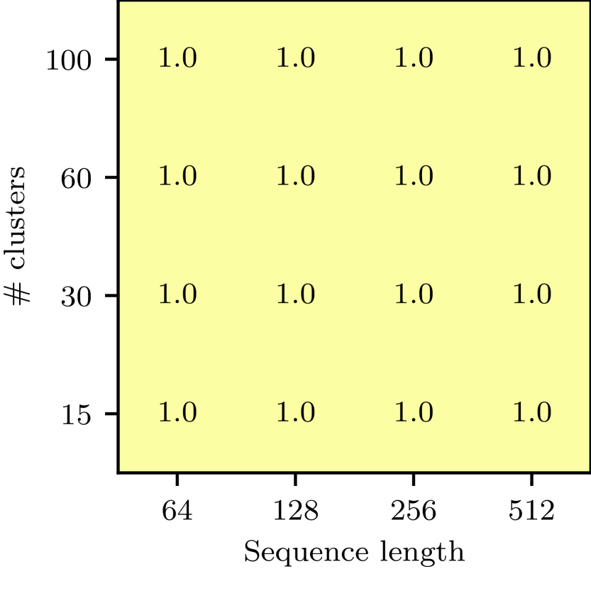
All transformer variants consist of layers, attention heads, embedding dimension of for each head, and feed-forward dimension of . For both clustered and improved clustered attention, we set the number of bits for LSH to and the number of Lloyd iterations for the K-Means to . Both clustered and improved clustered attention are trained with , , and clusters. We also train Reformer with , , and hashing rounds. Finally, all models are trained using R-Adam optimizer [15] with a learning rate of , batch size of for iterations.
In figure 5, we illustrate the results of this experiment as heatmaps depicting the achieved accuracy for a given combination of number of clusters and sequence length for clustered transformers and number of hashing rounds and sequence length for Reformer. Note that the vanilla transformer solves the task perfectly for all sequence lengths. We observe that both clustered (Fig. 5(b)) and Reformer (Fig. 5(c)) require more clusters or more rounds as the sequence length increases. However, improved clustered achieves the same performance as vanilla transformers, namely perfect accuracy, for every number of clusters and sequence length combination. This result increases our confidence that the required number of clusters for our method is not a function of the sequence length but of the task at hand.
C.3 Automatic Speech Recognition
In this section, we present the details for the ASR experiments such as transformer architecture, optimizer and learning rate schedule. As mentioned in the main paper, for i-clustered, unless specified, is set to 32. Furthermore, all transformers have heads with an embedding dimension of on each head and feed-forward dimension of . Other architectural details specific to experiments are described later.
C.3.1 Wall Street Journal
Convergence Behaviour:
For this experiment, we train transformer with full, clustered and Reformer attention variants. All models consist of layers. For Reformer, we train two variants with and rounds of hashing with chunk size fixed to as suggested. For clustered and improved clustered attention we set the number of clusters to . We also set the number of Lloyd iterations for K-Means to and the bits for LSH to . All models are trained to convergence using the R-Adam optimizer [15] with a learning rate of , max gradient norm set to and and weight decay of . The learning rate is dropped when the validation loss plateaus. For each model we select the largest batch size that fits the GPU. The full attention model was trained with a batch size of while the clustered variants: clustered and i-clustered could fit batch sizes of and respectively. For Reformer variants: lsh- and lsh-, batch sizes of and were used.
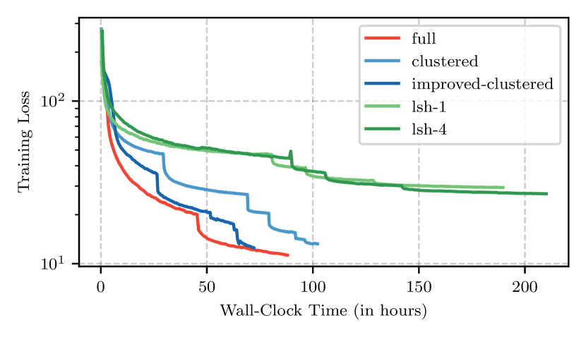
In figure 7(a), we show the training loss convergence for different transformer variants. It can be seen that i-clustered has a much faster convergence than the clustered attention. This shows that the improved clustered attention indeed approximates the full attention better. More importantly, only the i-clustered attention has a comparable wall-clock convergence. Given that full has a much smaller batch size, it make many more updates per-epoch. We think that a slightly smaller batchsize with more updates would have been a better choice for the clustered transformers w.r.t. the wall-clock convergence. This is reflected in the Switchboard experiments where the batchsizes for clustered variants were smaller due to more layers. Finally, as can be seen from the wall-clock convergence, the clustered transformers significantly outperform the Reformer variants.
Speed-Accuracy Tradeoff:
As described in the main paper, for this task we additionally train full with and layers. Similary, we train clustered with 9 layers, and and clusters. We also train an i-clustered model with 9 layer and clusters, and smaller models with 6 layers, and and clusters.
For clustered and i-clustered variants with 9 layers, we finetuned the previously described models trained with clusters. We finetuned for epochs with a learning rate of . We train full with and layers to convergence in a similar fashion to the full with layers described previously. Finally, for i-clustered, we first trained model with layers and clusters using the training strategy used for layers and clusters. We then finetuned this model for epochs using clusters and a learning rate of .
C.3.2 Switchboard
Convergence Behaviour:
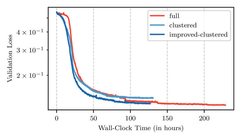
For this experiment, we train transformer with full and clustered attention variants. All models consist of layers. For clustered and improved clustered attention we set the number of clusters to . We also set the number of Lloyd iterations for K-Means to and the bits for LSH to .
Following common practice for flat-start lattice-free MMI training, we train over multiple gpus with weight averaging for synchronization as described in [23]. Specfically, we modify the e2e training recipe for the Wall Street Journal in Kaldi [22] with the following two key differences: first, the acoustic model training is done in PyTorch and second, we use R-Adam optimizer instead on natural stochastic gradient descent.
All models are trained using the R-Adam optimizer with a learning rate of , max gradient norm set to and and weight decay of . The learning rate is dropped when the validation loss plateaus. We use the word error rate (WER) on the validation set for early stopping and model selection. The full attention model is trained with a batch size of while the clustered variants: clustered and i-clustered are trained with a batch size of .
In figure 7(b), we show the training loss convergence for different transformer variants. It can be seen that i-clustered has the fastest convergence for this setup. Note that the overall training time for clustered attention is still less than that of full as it starts to overfit early on the validation set WER.
Speed-Accuracy Tradeoff:
For this task we additionally train full with and layers. Similary, we train clustered with 12 layers, and and clusters. We also train i-clustered with 12 layer and clusters, and smaller models with 8 layers, and and clusters.
For clustered and i-clustered variants with 12 layers, we finetuned the previously described models trained with clusters. We finetuned for epochs with a learning rate of . Once again, full with and layers were trained to convergence similar to full with layers described previously. Finally, for i-clustered with layers, we first train a model with clusters using the training strategy used for layers and clusters. We then finetuned this model for epochs using clusters and a learning rate of .
C.4 RoBERTa Approximation
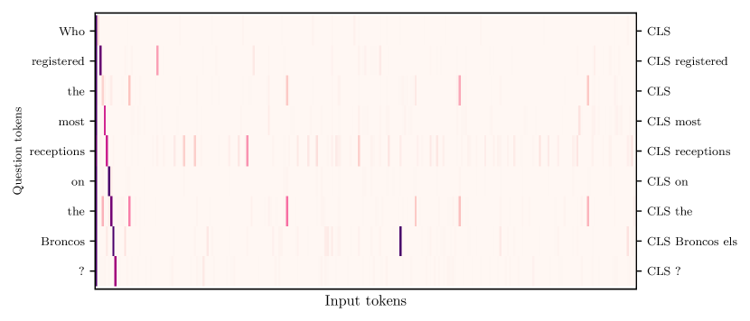
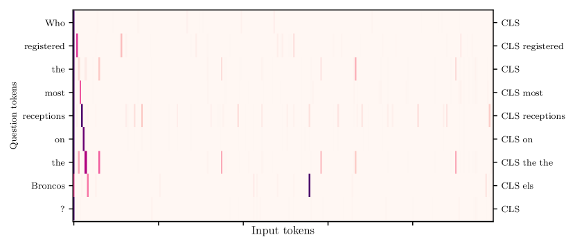
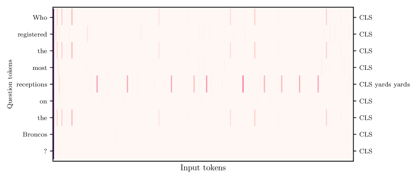
In this section we provide a qualitative comparison between the full attention, and the clustered attention variants clustered and i-clustered used for approximation. As described in main paper, we use clusters for both attention variants. In Figure 8 we show the attention distribution for the question tokens for a randomly selected question-context tuple from the SQuAD dataset. For each token in the question we show the attention distribution over the input sequence formed by concatenating question and context tokens with CLS and SEP tokens appended. It can be seen that with only few clusters, improved clustered approximates the full attention very closely even when the attention distribution has complicated and sparse patterns. In contrast, clustered attention fails to capture such attention distribution during approximation. Moreover, it can further be seen that for almost all question tokens, both full and improved clustered have the same tokens with the highest attention weights. This further strengthens our believe that improved clustered attention can approximate a wide range of complicated attention patterns.
Manning finished the year with a career-low 67.9 passer rating, throwing for 2,249 yards and nine touchdowns, with 17 interceptions. In contrast, Osweiler threw for 1,967 yards, 10 touchdowns and six interceptions for a rating of 86.4. Veteran receiver Demaryius Thomas led the team with 105 receptions for 1,304 yards and six touchdowns, while Emmanuel Sanders caught 76 passes for 1,135 yards and six scores, while adding another 106 yards returning punts. Tight end Owen Daniels was also a big element of the passing game with 46 receptions for 517 yards. Running back C. J. Anderson was the team’s leading rusher 863 yards and seven touchdowns, while also catching 25 passes for 183 yards. Running back Ronnie Hillman also made a big impact with 720 yards, five touchdowns, 24 receptions, and a 4.7 yards per carry average. Overall, the offense ranked 19th in scoring with 355 points and did not have any Pro Bowl selections.