A Bivariate Compound Dynamic Contagion Process for Cyber Insurance
Department of Actuarial Studies & Business Analytics, Macquarie
Business School, Macquarie University, Sydney NSW 2109, Australia, E-mail:
jiwook.jang@mq.edu.au
Institute of Mathematical Sciences, Ewha Womans University, Seoul, 03760,
Korea, E-mail: rosy.oh5@gmail.com
Abstract As corporates and governments become more digital, they
become vulnerable to various forms of cyber attack. Cyber insurance products
have been used as risk management tools, yet their pricing does not reflect
actual risk, including that of multiple, catastrophic and contagious losses.
For the modelling of aggregate losses from cyber events, in this paper we
introduce a bivariate compound dynamic contagion process, where the
bivariate dynamic contagion process is a point process that includes both
externally excited joint jumps, which are distributed according to a shot
noise Cox process and two separate self-excited jumps, which are distributed
according to the branching structure of a Hawkes process with an exponential
fertility rate, respectively. We analyse the theoretical distributional
properties for these processes systematically, based on the piecewise
deterministic Markov process developed by Davis (1984) and the univariate
dynamic contagion process theory developed by Dassios and Zhao (2011). The
analytic expression of the Laplace transform of the compound process and its
moments are presented, which have the potential to be applicable to a
variety of problems in credit, insurance, market and other operational
risks. As an application of this process, we provide insurance premium
calculations based on its moments. Numerical examples show that this
compound process can be used for the modelling of aggregate losses from
cyber events. We also provide the simulation algorithm for statistical
analysis, further business applications and research.
Keywords : Aggregate losses from cyber events; Contagion risk;
Bivariate compound dynamic contagion process; Hawkes process; Piecewise
deterministic Markov process; Martingale methodology; Insurance premium
Due to the digitalisation of business and economic activities via the
Internet of Things (IoT), cloud computing, mobile and other innovative
technologies, cyber risk is inherent and extreme. Cyber risks refer to any
risk of financial loss, disruption to operations, or damage to the
reputation of an organisation due to failure of its information technology
(IT) systems, as defined by the Institute of Risk Management (IRM).
Financial losses from malicious cyber activities result from IT
security/data/digital assets recovery, liability in respect of identity
theft and data breaches, reputation/brand damage, legal liability, cyber
extortion, regulatory defence and penalties coverage and business
interruption.
The frequency of malicious cyber activities is rapidly increasing, with the
scope and nature dependent on an organisation’s industry, size and location.
According to a 2016 Allianz survey, cyber risk is the top long-term risk to
business and currently a top-three global business risk. It is therefore
critical that corporations and governments focus on IT and network security
enhancement. Unless public and private sector organisations have effective
cyber security plans and strategies in place, and tools to manage and
mitigate losses from cyber risks, cyber events have the potential to affect
their business significantly, possibly damaging hard-earned reputations
irreparably.
Insurance has served to mitigate liability since the 17th century, after the
Great Fire of London in 1666. As part of a cyber risk mitigation strategy,
cyber insurance can be purchased by organisations to cover economic and
financial losses occurring from cyber incidents. Since the widespread Y2K
concerns raised the profile of the possible security vulnerabilities of
digitalisation, the cyber insurance industry has grown to a total annual
premium of $2.5 billion, and the market is expected to reach $20 billion
by 2025 globally. However, due to the complexity of cyber incidents, i.e.
multiple, catastrophic and contagious losses, it is difficult for insurers
to price cyber insurance products accurately. Inaccurate pricing could have
severe market effects in the event of a significant claim.
To date however there has been little theoretical work done on developing
acceptable cyber insurance pricing models. Also due to the complexity of
cyber risks, the previous studies (Mukhopadhyay et al. 2006; Herath and
Herath 2011and Xu and Hua 2017) do not provide a suitable framework to
measure cyber risks as they have not accounted for future cyber attacks
dynamically. Also traditionally insurance claim modelling has used
homogeneous/non-homogeneous Poisson processes as a claim arrival process.
However, for cyber events, the assumption that resulting claims occur in
terms of the Poisson process is inadequate due to its deterministic
intensity. Therefore, an alternative point process needs to be used to
predict claim arrivals from cyber incidents.
To this effect, we introduce a bivariate compound dynamic contagion
process (BCDCP) for the modelling of aggregate losses from cyber events,
where the bivariate dynamic contagion process (BDCP) is a point process
which has both externally excited joint jumps, which are distributed
according to a shot noise Cox process and two separate self-excited jumps,
which are Hawkes processes. Since Hawkes (1971a, 1971b) and Hawkes and Oakes
(1974) introduced a self-exciting point process, the applications and
modelling of Hawkes processes in finance and insurance can be found in
Chavez-Demoulin et al. (2005), McNeil et al. (2005), Bauwens and Hautsch
(2009), Bowsher (2007), Errais et al. (2010), Stabile and Torrisi (2010),
Embrechts et al. (2011), Giesecke and Kim (2011) and Aït-Sahalia et al.
(2014, 2015).
Dassios and Zhao (2011) introduced a dynamic contagion process, which is a
generalisation of the externally excited Cox process with shot noise
intensity and the self-excited Hawkes process applying to credit risk.
Dassios and Zhao (2012) also examined infinite horizon ruin probability with
its Monte Carlo simulation using this process as the claim arrival process.
Dassios and Zhao (2017a) extended this process with diffusion component to
calculate the default probability and to price defaultable zero-coupon
bonds. We have found dynamic contagion processes to be flexible and
realistic in modelling claims with contagion.
These aforementioned papers are neither the bivariate dynamic contagion
models nor the compound models. In contrast we extend it further to
quantify aggregate losses from cyber events using a bivariate compound dynamic contagion process as they are multiple, catastrophic and
contagious losses. Biener et al. (2015) emphasised that one of
characteristics of cyber risk is highly interrelated losses, and modelling
cyber risk would be a great deal of promise to test them when enough cyber
loss data become available.
Bivariate modelling with self-exciting Hawkes processes can be noticed in
Jang and Dassios (2013), where they introduced a bivariate shot noise
self-exciting process that can be used for the modelling of catastrophic
losses. Dong (2014) examined the stationarity of bivariate dynamic contagion
processes including the cross-exciting contagion effect in his doctoral
thesis. Applications and modelling of multivariate Hawkes process in
high-frequency limit order book data can be found in Rombaldi et al. (2017)
and Lu and Abergel (2018). Yang et al. (2018) investigated the
interactions between market return events and investor sentiment using a
multivariate Hawkes process.
Compound modelling with univariate self-exciting Hawkes processes can be
noticed in Dassios and Zhao (2017b), where they developed the algorithms for
a generalised self-exciting point process with CIR-type intensities. Gao
et al. (2018) applied the joint Laplace transform of the classical Hawkes
process and its compound process in dark pool trading, which do not display
bid and ask quotes to the public.
This project develops a new model for pricing cyber risk using a BCDCP,
which accommodate the interdependence dynamics of IT system and the
frequency and impact of cyber events. Our research offers a new framework
to enable insurance companies to price cyber insurance policies
accommodating clustering of losses.
This paper is structured as follows. In Section 2, we provide a mathematical
definition of the BCDCP and the BDCP, respectively via the stochastic
intensity representation adopted the one used by Dassios and Zhao (2011) and
the algorithm for simulating these processes in Section 5. In Section 3, we
analyse these processes systematically for their theoretical distributional
properties, based on the piecewise deterministic Markov process theory
developed by Davis (1984), and the martingale methodology used by Dassios
and Jang (2003). The joint moment of two processes, its covariance and
linear correlation are derived in Section 4, where for simplicity, we use
the case for the stationary distribution of the intensity processes. As an
application of this process, we provide cyber insurance premium calculations
based on these quantities in Section 5. Section 6 concludes the paper.
In this section, we have a mathematical definition for the BCDCP in
Definition 2.2. Before that, let us have a mathematical definition for the
BDCP in Definition 2.1 via the stochastic intensity representation adopted
the one used by Dassios and Zhao (2017). For an alternative definition for
this process, we refer you Dassios and Zhao (2011), Jang and Dassios (2013)
and Dong (2014), where they gave as a cluster process representation for the
univariate dynamic contagion process, the bivariate shot noise self-exciting
process and the bivariate dynamic contagion process, respectively.
Definition 2.1 (Bivariate dynamic contagion process). Bivariate
dynamic contagion process is a point process ( N t ( 1 ) N t ( 2 ) ) t > 0 = ( ∑ j ≥ 1 𝕀 ( T 2 , j ≤ t ) j = 1 , 2 , ⋯ ∑ k ≥ 1 𝕀 ( T 2 , k ≤ t ) k = 1 , 2 , ⋯ ) subscript superscript subscript 𝑁 𝑡 1 superscript subscript 𝑁 𝑡 2 𝑡 0 subscript 𝑗 1 𝕀 subscript subscript 𝑇 2 𝑗
𝑡 𝑗 1 2 ⋯
subscript 𝑘 1 𝕀 subscript subscript 𝑇 2 𝑘
𝑡 𝑘 1 2 ⋯
\left(\begin{array}[]{c}N_{t}^{\left(1\right)}\\
N_{t}^{\left(2\right)}\end{array}\right)_{t>0}=\left(\begin{array}[]{c}\sum\limits_{j\geq 1}\mathbb{I}\left(T_{2,j}\leq t\right)_{j=1,2,\cdots}\\
\sum\limits_{k\geq 1}\mathbb{I}\left(T_{2,k}\leq t\right)_{k=1,2,\cdots}\end{array}\right) ℑ t − limit-from subscript 𝑡 \Im_{t}- ( λ t ( 1 ) λ t ( 2 ) ) fragments λ 𝑡 1 fragments λ 𝑡 2 \left(\begin{tabular}[]{l}$\lambda_{t}^{\left(1\right)}$\\
$\lambda_{t}^{\left(2\right)}$\end{tabular}\right)
• { ℑ t } t ≥ 0 subscript subscript 𝑡 𝑡 0 \left\{\Im_{t}\right\}_{t\geq 0} ( N t ( 1 ) N t ( 2 ) ) , fragments N 𝑡 1 fragments N 𝑡 2 \left(\begin{tabular}[]{l}$N_{t}^{\left(1\right)}$\\
$N_{t}^{\left(2\right)}$\end{tabular}\right), { λ t ( 1 ) λ t ( 2 ) } t ≥ 0 subscript fragments λ 𝑡 1 fragments λ 𝑡 2 𝑡 0 \left\{\begin{tabular}[]{l}$\lambda_{t}^{\left(1\right)}$\\
$\lambda_{t}^{\left(2\right)}$\end{tabular}\right\}_{t\geq 0}
• λ 0 ( d ) superscript subscript 𝜆 0 𝑑 \lambda_{0}^{\left(d\right)} > 0 absent 0 >0 t = 0 𝑡 0 t=0 d = 1 , 2 𝑑 1 2
d=1,2
• a ( d ) superscript 𝑎 𝑑 a^{\left(d\right)} ≥ 0 absent 0 \geq 0
• δ ( d ) superscript 𝛿 𝑑 \delta^{\left(d\right)} > 0 absent 0 >0
• { X i ( 1 ) , X i ( 2 ) } i = 1 , 2 , ⋯ subscript superscript subscript 𝑋 𝑖 1 superscript subscript 𝑋 𝑖 2 𝑖 1 2 ⋯
\left\{X_{i}^{\left(1\right)},\text{ }X_{i}^{\left(2\right)}\right\}_{i=1,2,\cdots} i .i .d . positive externally-excited joint jumps with
distribution F ( x ( 1 ) , x ( 2 ) ) , 𝐹 superscript 𝑥 1 superscript 𝑥 2 F(x^{\left(1\right)},x^{\left(2\right)}), x ( 1 ) > 0 , superscript 𝑥 1 0 x^{\left(1\right)}>0, x ( 2 ) > 0 superscript 𝑥 2 0 x^{\left(2\right)}>0 F X ( 1 ) subscript 𝐹 superscript 𝑋 1 F_{X^{\left(1\right)}} F X ( 2 ) subscript 𝐹 superscript 𝑋 2 F_{X^{\left(2\right)}} { T 1 , i } i = 1 , 2 , ⋯ subscript subscript 𝑇 1 𝑖
𝑖 1 2 ⋯
\left\{T_{1,i}\right\}_{i=1,2,\cdots} M t subscript 𝑀 𝑡 M_{t} ρ > 0 𝜌 0 \rho>0 𝕀 𝕀 \mathbb{I}
• { Y j } j = 1 , 2 , ⋯ subscript subscript 𝑌 𝑗 𝑗 1 2 ⋯
\left\{Y_{j}\right\}_{j=1,2,\cdots} i .i .d . positive self-excited jumps with
distribution function G ( y ) 𝐺 𝑦 G(y) y > 0 𝑦 0 y>0 { T 2 , j } j = 1 , 2 , ⋯ subscript subscript 𝑇 2 𝑗
𝑗 1 2 ⋯
\left\{T_{2,j}\right\}_{j=1,2,\cdots}
• { Z k } k = 1 , 2 , ⋯ subscript subscript 𝑍 𝑘 𝑘 1 2 ⋯
\left\{Z_{k}\right\}_{k=1,2,\cdots} i .i .d . positive self-excited jumps with
distribution function H ( z ) 𝐻 𝑧 H(z) z > 0 𝑧 0 z>0 { T 2 , k } k = 1 , 2 , ⋯ subscript subscript 𝑇 2 𝑘
𝑘 1 2 ⋯
\left\{T_{2,k}\right\}_{k=1,2,\cdots}
• { X i ( 1 ) , X i ( 2 ) } i = 1 , 2 , ⋯ subscript superscript subscript 𝑋 𝑖 1 superscript subscript 𝑋 𝑖 2 𝑖 1 2 ⋯
\left\{X_{i}^{\left(1\right)},X_{i}^{\left(2\right)}\right\}_{i=1,2,\cdots} { Y j } j = 1 , 2 , ⋯ subscript subscript 𝑌 𝑗 𝑗 1 2 ⋯
\left\{Y_{j}\right\}_{j=1,2,\cdots} { Z k } k = 1 , 2 , ⋯ subscript subscript 𝑍 𝑘 𝑘 1 2 ⋯
\left\{Z_{k}\right\}_{k=1,2,\cdots} { T 1 , i } i = 1 , 2 , ⋯ subscript subscript 𝑇 1 𝑖
𝑖 1 2 ⋯
\left\{T_{1,i}\right\}_{i=1,2,\cdots} { T 2 , j } j = 1 , 2 , ⋯ subscript subscript 𝑇 2 𝑗
𝑗 1 2 ⋯
\left\{T_{2,j}\right\}_{j=1,2,\cdots} { T 2 , k } k = 1 , 2 , ⋯ subscript subscript 𝑇 2 𝑘
𝑘 1 2 ⋯
\left\{T_{2,k}\right\}_{k=1,2,\cdots}
The bivariate compound model we consider has the following
structure:
L t ( 1 ) superscript subscript 𝐿 𝑡 1 \displaystyle L_{t}^{(1)} = \displaystyle= ∑ j ≥ 1 Ξ j ( 1 ) 𝕀 ( T 2 , j ≤ t ) , subscript 𝑗 1 superscript subscript Ξ 𝑗 1 𝕀 subscript 𝑇 2 𝑗
𝑡
\displaystyle\sum\limits_{j\geq 1}\Xi_{j}^{\left(1\right)}\mathbb{I}\left(T_{2,j}\leq t\right),\text{ }
L t ( 2 ) superscript subscript 𝐿 𝑡 2 \displaystyle L_{t}^{(2)} = \displaystyle= ∑ k ≥ 1 Ξ k ( 2 ) 𝕀 ( T 2 , k ≤ t ) , \TCItag 2.2 subscript 𝑘 1 superscript subscript Ξ 𝑘 2 𝕀 subscript 𝑇 2 𝑘
𝑡 \TCItag 2.2
\displaystyle\sum\limits_{k\geq 1}\Xi_{k}^{\left(2\right)}\mathbb{I}\left(T_{2,k}\leq t\right),\TCItag{2.2} (6)
where L t ( d ) superscript subscript 𝐿 𝑡 𝑑 L_{t}^{(d)} d = 1 , 2 𝑑 1 2
d=1,2 N t ( d ) superscript subscript 𝑁 𝑡 𝑑 N_{t}^{\left(d\right)} t 𝑡 t Ξ j ( 1 ) superscript subscript Ξ 𝑗 1 \Xi_{j}^{\left(1\right)} Ξ k ( 2 ) superscript subscript Ξ 𝑘 2 \Xi_{k}^{\left(2\right)} J Y ( 1 ) subscript 𝐽 superscript 𝑌 1 J_{Y^{\left(1\right)}} K Y ( 2 ) subscript 𝐾 superscript 𝑌 2 K_{Y^{\left(2\right)}} N t ( 1 ) superscript subscript 𝑁 𝑡 1 N_{t}^{\left(1\right)} N t ( 2 ) superscript subscript 𝑁 𝑡 2 N_{t}^{\left(2\right)}
Definition 2.2 (Bivariate compound dynamic contagion process). Bivariate compound dynamic contagion process is a compound point
process ( L t ( 1 ) L t ( 2 ) ) t > 0 = ( ∑ j ≥ 1 Ξ j ( 1 ) 𝕀 ( T 2 , j ≤ t ) j = 1 , 2 , ⋯ ∑ k ≥ 1 Ξ k ( 2 ) 𝕀 ( T 2 , k ≤ t ) k = 1 , 2 , ⋯ ) subscript superscript subscript 𝐿 𝑡 1 superscript subscript 𝐿 𝑡 2 𝑡 0 subscript 𝑗 1 superscript subscript Ξ 𝑗 1 𝕀 subscript subscript 𝑇 2 𝑗
𝑡 𝑗 1 2 ⋯
subscript 𝑘 1 superscript subscript Ξ 𝑘 2 𝕀 subscript subscript 𝑇 2 𝑘
𝑡 𝑘 1 2 ⋯
\left(\begin{array}[]{c}L_{t}^{\left(1\right)}\\
L_{t}^{\left(2\right)}\end{array}\right)_{t>0}=\left(\begin{array}[]{c}\sum\limits_{j\geq 1}\Xi_{j}^{\left(1\right)}\mathbb{I}\left(T_{2,j}\leq t\right)_{j=1,2,\cdots}\\
\sum\limits_{k\geq 1}\Xi_{k}^{\left(2\right)}\mathbb{I}\left(T_{2,k}\leq t\right)_{k=1,2,\cdots}\end{array}\right) ℑ t − limit-from subscript 𝑡 \Im_{t}- ( λ t ( 1 ) λ t ( 2 ) ) fragments λ 𝑡 1 fragments λ 𝑡 2 \left(\begin{tabular}[]{l}$\lambda_{t}^{\left(1\right)}$\\
$\lambda_{t}^{\left(2\right)}$\end{tabular}\right)
• { Ξ j ( 1 ) } j = 1 , 2 , ⋯ subscript superscript subscript Ξ 𝑗 1 𝑗 1 2 ⋯
\left\{\Xi_{j}^{\left(1\right)}\right\}_{j=1,2,\cdots} i .i .d . positive individual
claim/loss amounts from risk type d = 1 𝑑 1 d=1 J ( ξ ( 1 ) ) 𝐽 superscript 𝜉 1 J(\xi^{\left(1\right)}) ξ ( 1 ) > 0 superscript 𝜉 1 0 \xi^{\left(1\right)}>0 { T 2 , j } j = 1 , 2 , ⋯ subscript subscript 𝑇 2 𝑗
𝑗 1 2 ⋯
\left\{T_{2,j}\right\}_{j=1,2,\cdots}
• { Ξ k ( 2 ) } k = 1 , 2 , ⋯ subscript superscript subscript Ξ 𝑘 2 𝑘 1 2 ⋯
\left\{\Xi_{k}^{\left(2\right)}\right\}_{k=1,2,\cdots} i .i .d . positive individual
claim/loss amounts from risk type d = 2 𝑑 2 d=2 K ( ξ ( 2 ) ) 𝐾 superscript 𝜉 2 K(\xi^{\left(2\right)}) ξ ( 2 ) > 0 superscript 𝜉 2 0 \xi^{\left(2\right)}>0 { T 2 , k } k = 1 , 2 , ⋯ subscript subscript 𝑇 2 𝑘
𝑘 1 2 ⋯
\left\{T_{2,k}\right\}_{k=1,2,\cdots}
• { X i ( 1 ) , X i ( 2 ) } i = 1 , 2 , ⋯ subscript superscript subscript 𝑋 𝑖 1 superscript subscript 𝑋 𝑖 2 𝑖 1 2 ⋯
\left\{X_{i}^{\left(1\right)},X_{i}^{\left(2\right)}\right\}_{i=1,2,\cdots} { Y j } j = 1 , 2 , ⋯ subscript subscript 𝑌 𝑗 𝑗 1 2 ⋯
\left\{Y_{j}\right\}_{j=1,2,\cdots} { Z k } k = 1 , 2 , ⋯ subscript subscript 𝑍 𝑘 𝑘 1 2 ⋯
\left\{Z_{k}\right\}_{k=1,2,\cdots} { Ξ j ( 1 ) } j = 1 , 2 , ⋯ subscript superscript subscript Ξ 𝑗 1 𝑗 1 2 ⋯
\left\{\Xi_{j}^{\left(1\right)}\right\}_{j=1,2,\cdots} { Ξ k ( 1 ) } k = 1 , 2 , ⋯ subscript superscript subscript Ξ 𝑘 1 𝑘 1 2 ⋯
\left\{\Xi_{k}^{\left(1\right)}\right\}_{k=1,2,\cdots} { T 1 , i } i = 1 , 2 , ⋯ subscript subscript 𝑇 1 𝑖
𝑖 1 2 ⋯
\left\{T_{1,i}\right\}_{i=1,2,\cdots} { T 2 , j } j = 1 , 2 , ⋯ subscript subscript 𝑇 2 𝑗
𝑗 1 2 ⋯
\left\{T_{2,j}\right\}_{j=1,2,\cdots} { T 2 , k } k = 1 , 2 , ⋯ subscript subscript 𝑇 2 𝑘
𝑘 1 2 ⋯
\left\{T_{2,k}\right\}_{k=1,2,\cdots}
The joint process of { ( λ t ( 1 ) λ t ( 2 ) ) , ( N t ( 1 ) N t ( 2 ) ) , ( L t ( 1 ) L t ( 2 ) ) } t ≥ 0 subscript fragments λ 𝑡 1 fragments λ 𝑡 2 superscript subscript 𝑁 𝑡 1 superscript subscript 𝑁 𝑡 2 superscript subscript 𝐿 𝑡 1 superscript subscript 𝐿 𝑡 2 𝑡 0 \left\{\left(\begin{tabular}[]{l}$\lambda_{t}^{\left(1\right)}$\\
$\lambda_{t}^{\left(2\right)}$\end{tabular}\right),\left(\begin{array}[]{c}N_{t}^{\left(1\right)}\\
N_{t}^{\left(2\right)}\end{array}\right),\left(\begin{array}[]{c}L_{t}^{\left(1\right)}\\
L_{t}^{\left(2\right)}\end{array}\right)\right\}_{t\geq 0} ℝ + × ℕ 0 × ℝ 0 + superscript ℝ subscript ℕ 0 superscript subscript ℝ 0 \mathbb{R}^{+}\times\mathbb{N}_{0}\times\mathbb{R}_{0}^{+} ( λ t ( 1 ) , N t ( 1 ) , L t ( 1 ) , λ t ( 2 ) , N t ( 2 ) , L t ( 2 ) , t ) superscript subscript 𝜆 𝑡 1 superscript subscript 𝑁 𝑡 1 superscript subscript 𝐿 𝑡 1 superscript subscript 𝜆 𝑡 2 superscript subscript 𝑁 𝑡 2 superscript subscript 𝐿 𝑡 2 𝑡 \left(\lambda_{t}^{\left(1\right)},N_{t}^{\left(1\right)},L_{t}^{(1)},\lambda_{t}^{\left(2\right)},N_{t}^{\left(2\right)},L_{t}^{(2)},t\right) f ( λ ( 1 ) , n ( 1 ) , l ( 1 ) , λ ( 2 ) , n ( 2 ) , l ( 2 ) , t ) 𝑓 superscript 𝜆 1 superscript 𝑛 1 superscript 𝑙 1 superscript 𝜆 2 superscript 𝑛 2 superscript 𝑙 2 𝑡 f\left(\lambda^{\left(1\right)},n^{\left(1\right)},l^{(1)},\lambda^{\left(2\right)},n^{\left(2\right)},l^{(2)},t\right) 𝒟 ( 𝒜 ) 𝒟 𝒜 \mathcal{D}\left(\mathcal{A}\right)
𝒜 f ( λ ( 1 ) , n ( 1 ) , l ( 1 ) , λ ( 2 ) , n ( 2 ) , l ( 2 ) , t ) 𝒜 𝑓 superscript 𝜆 1 superscript 𝑛 1 superscript 𝑙 1 superscript 𝜆 2 superscript 𝑛 2 superscript 𝑙 2 𝑡 \displaystyle\mathcal{A}\text{ }f\left(\lambda^{\left(1\right)},n^{\left(1\right)},l^{(1)},\lambda^{\left(2\right)},n^{\left(2\right)},l^{(2)},t\right) (28)
= \displaystyle= ∂ f ∂ t + δ ( 1 ) ( a ( 1 ) − λ ( 1 ) ) ∂ f ∂ λ ( 1 ) + δ ( 2 ) ( a ( 2 ) − λ ( 2 ) ) ∂ f ∂ λ ( 2 ) 𝑓 𝑡 superscript 𝛿 1 superscript 𝑎 1 superscript 𝜆 1 𝑓 superscript 𝜆 1 superscript 𝛿 2 superscript 𝑎 2 superscript 𝜆 2 𝑓 superscript 𝜆 2 \displaystyle\frac{\partial f}{\partial t}+\delta^{\left(1\right)}\left(a^{\left(1\right)}-\lambda^{\left(1\right)}\right)\frac{\partial f}{\partial\lambda^{\left(1\right)}}+\delta^{\left(2\right)}\left(a^{\left(2\right)}-\lambda^{\left(2\right)}\right)\frac{\partial f}{\partial\lambda^{\left(2\right)}}
+ λ ( 1 ) [ ∫ 0 ∞ ∫ 0 ∞ f ( λ ( 1 ) + y , n ( 1 ) + 1 , l ( 1 ) + ξ ( 1 ) , λ ( 2 ) , n ( 2 ) , l ( 2 ) , t ) 𝑑 G ( y ) 𝑑 J ( ξ ( 1 ) ) − f ( λ ( 1 ) , n ( 1 ) , l ( 1 ) , λ ( 2 ) , n ( 2 ) , l ( 2 ) , t ) ] superscript 𝜆 1 delimited-[] superscript subscript 0 superscript subscript 0 𝑓 superscript 𝜆 1 𝑦 superscript 𝑛 1 1 superscript 𝑙 1 superscript 𝜉 1 superscript 𝜆 2 superscript 𝑛 2 superscript 𝑙 2 𝑡 differential-d 𝐺 𝑦 differential-d 𝐽 superscript 𝜉 1 𝑓 superscript 𝜆 1 superscript 𝑛 1 superscript 𝑙 1 superscript 𝜆 2 superscript 𝑛 2 superscript 𝑙 2 𝑡 \displaystyle+\lambda^{\left(1\right)}\left[\begin{array}[]{c}\int\limits_{0}^{\infty}\int\limits_{0}^{\infty}f\left(\lambda^{\left(1\right)}+y,n^{\left(1\right)}+1,l^{(1)}+\xi^{\left(1\right)},\lambda^{\left(2\right)},n^{\left(2\right)},l^{(2)},t\right)dG(y)dJ(\xi^{\left(1\right)})\\
-f\left(\lambda^{\left(1\right)},n^{\left(1\right)},l^{(1)},\lambda^{\left(2\right)},n^{\left(2\right)},l^{(2)},t\right)\end{array}\right]
+ λ ( 2 ) [ ∫ 0 ∞ ∫ 0 ∞ f ( λ ( 1 ) , n ( 1 ) , l ( 1 ) , λ ( 2 ) + z , n ( 2 ) + 1 , l ( 2 ) + ξ ( 2 ) , t ) 𝑑 H ( z ) 𝑑 K ( ξ ( 2 ) ) − f ( λ ( 1 ) , n ( 1 ) , l ( 1 ) , λ ( 2 ) , n ( 2 ) , l ( 2 ) , t ) ] superscript 𝜆 2 delimited-[] superscript subscript 0 superscript subscript 0 𝑓 superscript 𝜆 1 superscript 𝑛 1 superscript 𝑙 1 superscript 𝜆 2 𝑧 superscript 𝑛 2 1 superscript 𝑙 2 superscript 𝜉 2 𝑡 differential-d 𝐻 𝑧 differential-d 𝐾 superscript 𝜉 2 𝑓 superscript 𝜆 1 superscript 𝑛 1 superscript 𝑙 1 superscript 𝜆 2 superscript 𝑛 2 superscript 𝑙 2 𝑡 \displaystyle+\lambda^{\left(2\right)}\left[\begin{array}[]{c}\int\limits_{0}^{\infty}\int\limits_{0}^{\infty}f\left(\lambda^{\left(1\right)},n^{\left(1\right)},l^{(1)},\lambda^{\left(2\right)}+z,n^{\left(2\right)}+1,l^{(2)}+\xi^{\left(2\right)},t\right)dH(z)dK(\xi^{\left(2\right)})\\
-f\left(\lambda^{\left(1\right)},n^{\left(1\right)},l^{(1)},\lambda^{\left(2\right)},n^{\left(2\right)},l^{(2)},t\right)\end{array}\right]
+ ρ [ ∫ 0 ∞ ∫ 0 ∞ f ( λ ( 1 ) + x ( 1 ) , n ( 1 ) , l ( 1 ) , λ ( 2 ) + x ( 2 ) , n ( 2 ) , l ( 2 ) , t ) 𝑑 F X ( 1 ) , X ( 2 ) ( x ( 1 ) , x ( 2 ) ) − f ( λ ( 1 ) , n ( 1 ) , l ( 1 ) , λ ( 2 ) , n ( 2 ) , l ( 2 ) , t ) ] , 𝜌 delimited-[] superscript subscript 0 superscript subscript 0 𝑓 superscript 𝜆 1 superscript 𝑥 1 superscript 𝑛 1 superscript 𝑙 1 superscript 𝜆 2 superscript 𝑥 2 superscript 𝑛 2 superscript 𝑙 2 𝑡 differential-d subscript 𝐹 superscript 𝑋 1 superscript 𝑋 2
superscript 𝑥 1 , superscript 𝑥 2 𝑓 superscript 𝜆 1 superscript 𝑛 1 superscript 𝑙 1 superscript 𝜆 2 superscript 𝑛 2 superscript 𝑙 2 𝑡 \displaystyle+\rho\left[\begin{array}[]{c}\int\limits_{0}^{\infty}\int\limits_{0}^{\infty}f\left(\lambda^{\left(1\right)}+x^{\left(1\right)},n^{\left(1\right)},l^{(1)},\lambda^{\left(2\right)}+x^{\left(2\right)},n^{\left(2\right)},l^{(2)},t\right)dF_{X^{\left(1\right)},X^{\left(2\right)}}(x^{\left(1\right)}\text{, }x^{\left(2\right)})\\
-f\left(\lambda^{\left(1\right)},n^{\left(1\right)},l^{(1)},\lambda^{\left(2\right)},n^{\left(2\right)},l^{(2)},t\right)\end{array}\right],
\TCItag 2.3 \TCItag 2.3 \displaystyle\TCItag{2.3}
where 𝒟 ( 𝒜 ) 𝒟 𝒜 \mathcal{D}\left(\mathcal{A}\right) 𝒜 𝒜 \mathcal{A} f ( λ ( 1 ) , n ( 1 ) , l ( 1 ) , λ ( 2 ) , n ( 2 ) , l ( 2 ) , t ) 𝑓 superscript 𝜆 1 superscript 𝑛 1 superscript 𝑙 1 superscript 𝜆 2 superscript 𝑛 2 superscript 𝑙 2 𝑡 f\left(\lambda^{\left(1\right)},n^{\left(1\right)},l^{(1)},\lambda^{\left(2\right)},n^{\left(2\right)},l^{(2)},t\right) λ ( 1 ) , λ ( 2 ) superscript 𝜆 1 superscript 𝜆 2
\lambda^{\left(1\right)},\lambda^{\left(2\right)} t 𝑡 t λ ( 1 ) , λ ( 2 ) superscript 𝜆 1 superscript 𝜆 2
\lambda^{\left(1\right)},\lambda^{\left(2\right)} t , 𝑡 t,
| ∫ 0 ∞ ∫ 0 ∞ f ( ⋅ , λ ( 1 ) + y , n ( 1 ) + 1 , l ( 1 ) + ξ ( 1 ) , ⋅ ) 𝑑 G ( y ) 𝑑 J ( ξ ( 1 ) ) − f ( ⋅ , λ ( 1 ) , n ( 1 ) , l ( 1 ) , ⋅ ) | < ∞ , superscript subscript 0 superscript subscript 0 𝑓 ⋅ superscript 𝜆 1 𝑦 superscript 𝑛 1 1 superscript 𝑙 1 superscript 𝜉 1 ⋅ differential-d 𝐺 𝑦 differential-d 𝐽 superscript 𝜉 1 𝑓 ⋅ superscript 𝜆 1 superscript 𝑛 1 superscript 𝑙 1 ⋅ , \left|\int\limits_{0}^{\infty}\int\limits_{0}^{\infty}f\left(\cdot,\lambda^{\left(1\right)}+y,n^{\left(1\right)}+1,l^{(1)}+\xi^{\left(1\right)},\cdot\right)dG(y)dJ(\xi^{\left(1\right)})-f\left(\cdot,\lambda^{\left(1\right)},n^{\left(1\right)},l^{(1)},\cdot\right)\right|<\infty\text{,}
| ∫ 0 ∞ ∫ 0 ∞ f ( ⋅ , λ ( 2 ) + z , n ( 2 ) + 1 , l ( 2 ) + ξ ( 2 ) , ⋅ ) 𝑑 H ( z ) 𝑑 K ( ξ ( 2 ) ) − f ( ⋅ , λ ( 2 ) , n ( 2 ) , l ( 2 ) , ⋅ ) | < ∞ , superscript subscript 0 superscript subscript 0 𝑓 ⋅ superscript 𝜆 2 𝑧 superscript 𝑛 2 1 superscript 𝑙 2 superscript 𝜉 2 ⋅ differential-d 𝐻 𝑧 differential-d 𝐾 superscript 𝜉 2 𝑓 ⋅ superscript 𝜆 2 superscript 𝑛 2 superscript 𝑙 2 ⋅ \left|\int\limits_{0}^{\infty}\int\limits_{0}^{\infty}f\left(\cdot,\lambda^{\left(2\right)}+z,n^{\left(2\right)}+1,l^{(2)}+\xi^{\left(2\right)},\cdot\right)dH(z)dK(\xi^{\left(2\right)})-f\left(\cdot,\lambda^{\left(2\right)},n^{\left(2\right)},l^{(2)},\cdot\right)\right|<\infty,
| ∫ 0 ∞ ∫ 0 ∞ f ( ⋅ , λ ( 1 ) + x ( 1 ) , λ ( 2 ) + x ( 2 ) , ⋅ ) 𝑑 F ( x ( 1 ) , x ( 2 ) ) − f ( ⋅ , λ ( 1 ) + x ( 1 ) , λ ( 2 ) + x ( 2 ) , ⋅ ) | < ∞ . superscript subscript 0 superscript subscript 0 𝑓 ⋅ superscript 𝜆 1 superscript 𝑥 1 superscript 𝜆 2 superscript 𝑥 2 ⋅ differential-d 𝐹 superscript 𝑥 1 superscript 𝑥 2 𝑓 ⋅ superscript 𝜆 1 superscript 𝑥 1 superscript 𝜆 2 superscript 𝑥 2 ⋅ . \left|\int\limits_{0}^{\infty}\int\limits_{0}^{\infty}f\left(\cdot,\lambda^{\left(1\right)}+x^{\left(1\right)},\lambda^{\left(2\right)}+x^{\left(2\right)},\cdot\right)dF\left(x^{\left(1\right)},x^{\left(2\right)}\right)-f\left(\cdot,\lambda^{\left(1\right)}+x^{\left(1\right)},\lambda^{\left(2\right)}+x^{\left(2\right)},\cdot\right)\right|<\infty\text{.}
3. Bivariate Compound Dynamic Contagion Process
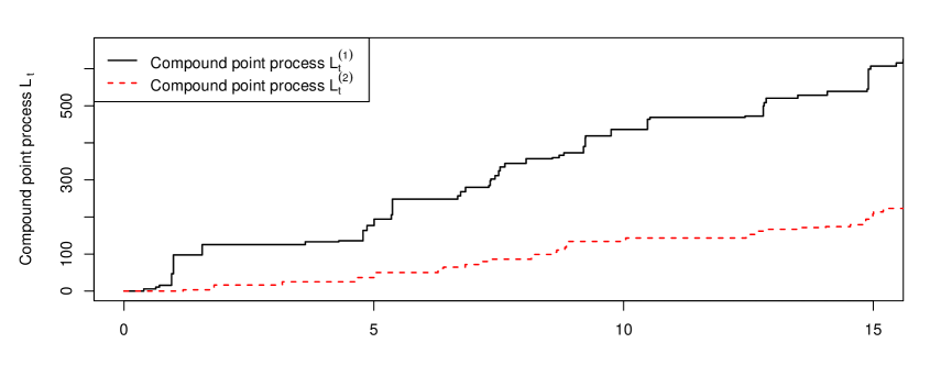
In this section, we derive the joint Laplace transform of the process ( L T ( 1 ) , (L_{T}^{\left(1\right)}, L T ( 2 ) ) L_{T}^{\left(2\right)}) ( N T ( 1 ) , (N_{T}^{\left(1\right)}, N T ( 2 ) ) N_{T}^{\left(2\right)}) ( λ T ( 1 ) , (\lambda_{T}^{\left(1\right)}, λ T ( 2 ) ) \lambda_{T}^{\left(2\right)})
3.1. Joint Laplace Transform - Probability Generating Function of
( λ t ( 1 ) , (\lambda_{t}^{\left(1\right)}, λ t ( 2 ) , superscript subscript 𝜆 𝑡 2 \lambda_{t}^{\left(2\right)}, N t ( 1 ) , superscript subscript 𝑁 𝑡 1 N_{t}^{\left(1\right)}, N t ( 2 ) , superscript subscript 𝑁 𝑡 2 N_{t}^{\left(2\right)}, L t ( 1 ) , superscript subscript 𝐿 𝑡 1 L_{t}^{\left(1\right)}, L t ( 2 ) ) L_{t}^{\left(2\right)})
Theorem 3.1 Considering the constants , 0 ≤ θ ≤ 1 , 0 𝜃 1 0\leq\theta\leq 1, 0 ≤ η ≤ 1 , 0 𝜂 1 0\leq\eta\leq 1, ν ≥ 0 , 𝜈 0 \nu\geq 0, ζ ≥ 0 , 𝜁 0 \zeta\geq 0, υ ≥ 0 , 𝜐 0 \upsilon\geq 0, γ ≥ 0 𝛾 0 \gamma\geq 0 and time 0 ≤ t ≤ T , 0 𝑡 𝑇 0\leq t\leq T, we have the
conditional joint Laplace transform , probability generating
function of the process ( λ T ( 1 ) , (\lambda_{T}^{\left(1\right)}, λ T ( 2 ) ) \lambda_{T}^{\left(2\right)}) the point process (N T ( 1 ) , superscript subscript 𝑁 𝑇 1 N_{T}^{\left(1\right)}, N T ( 2 ) ) N_{T}^{\left(2\right)}) and the
compound point process ( L T ( 1 ) , (L_{T}^{\left(1\right)}, L T ( 2 ) ) L_{T}^{\left(2\right)}) is given by
E [ θ { N T ( 1 ) − N t ( 1 ) } η { N T ( 2 ) − N t ( 2 ) } e − ν { L T ( 1 ) − L t ( 1 ) } e − ζ { L T ( 2 ) − L t ( 2 ) } × e − υ λ T ( 1 ) e − γ λ T ( 2 ) ∣ ℑ t ] 𝐸 delimited-[] conditional superscript 𝜃 superscript subscript 𝑁 𝑇 1 superscript subscript 𝑁 𝑡 1 superscript 𝜂 superscript subscript 𝑁 𝑇 2 superscript subscript 𝑁 𝑡 2 superscript 𝑒 𝜈 superscript subscript 𝐿 𝑇 1 superscript subscript 𝐿 𝑡 1 superscript 𝑒 𝜁 superscript subscript 𝐿 𝑇 2 superscript subscript 𝐿 𝑡 2 superscript 𝑒 𝜐 superscript subscript 𝜆 𝑇 1 superscript 𝑒 𝛾 superscript subscript 𝜆 𝑇 2 subscript 𝑡 \displaystyle E\left[\theta^{\left\{N_{T}^{\left(1\right)}-N_{t}^{\left(1\right)}\right\}}\eta^{\left\{N_{T}^{\left(2\right)}-N_{t}^{\left(2\right)}\right\}}e^{-\nu\left\{L_{T}^{\left(1\right)}-L_{t}^{\left(1\right)}\right\}}e^{-\zeta\left\{L_{T}^{\left(2\right)}-L_{t}^{\left(2\right)}\right\}}\times e^{-\upsilon\lambda_{T}^{\left(1\right)}}e^{-\gamma\lambda_{T}^{\left(2\right)}}\mid\Im_{t}\right] (29)
= \displaystyle= e − B 1 ( t ) λ t ( 1 ) e − B 2 ( t ) λ t ( 2 ) e − { C ( T ) − C ( t ) } , \TCItag 3.1 superscript 𝑒 subscript 𝐵 1 𝑡 superscript subscript 𝜆 𝑡 1 superscript 𝑒 subscript 𝐵 2 𝑡 superscript subscript 𝜆 𝑡 2 superscript 𝑒 𝐶 𝑇 𝐶 𝑡 \TCItag 3.1
\displaystyle e^{-B_{1}(t)\lambda_{t}^{\left(1\right)}}e^{-B_{2}(t)\lambda_{t}^{\left(2\right)}}e^{-\left\{C(T)-C(t)\right\}},\TCItag{3.1}
where B 1 ( t ) subscript 𝐵 1 𝑡 B_{1}(t) and B 2 ( t ) subscript 𝐵 2 𝑡 B_{2}(t) are determined by
two non-linear ordinary differential equations (ODEs )
− B 1 ′ ( t ) + δ ( 1 ) B 1 ( t ) + θ g ∧ { B 1 ( t ) } j ∧ ( ν ) − 1 superscript subscript 𝐵 1 ′ 𝑡 superscript 𝛿 1 subscript 𝐵 1 𝑡 𝜃 𝑔 subscript 𝐵 1 𝑡 𝑗 𝜈 1 \displaystyle-B_{1}^{\prime}\left(t\right)+\delta^{\left(1\right)}B_{1}\left(t\right)+\theta\text{ }\overset{\wedge}{g}\left\{B_{1}\left(t\right)\right\}\text{ }\overset{\wedge}{j}\left(\nu\right)-1 = \displaystyle= 0 , \TCItag 3.2 0 \TCItag 3.2
\displaystyle 0,\TCItag{3.2} (30)
− B 2 ′ ( t ) + δ ( 2 ) B 2 ( t ) + η h ∧ { B 2 ( t ) } k ∧ ( ζ ) − 1 superscript subscript 𝐵 2 ′ 𝑡 superscript 𝛿 2 subscript 𝐵 2 𝑡 𝜂 ℎ subscript 𝐵 2 𝑡 𝑘 𝜁 1 \displaystyle-B_{2}^{\prime}\left(t\right)+\delta^{\left(2\right)}B_{2}\left(t\right)+\eta\text{ }\overset{\wedge}{h}\left\{B_{2}\left(t\right)\right\}\text{ }\overset{\wedge}{k}\left(\zeta\right)-1 = \displaystyle= 0 , \TCItag 3.3 0 \TCItag 3.3
\displaystyle 0,\TCItag{3.3} (31)
with the boundary condition B 1 ( T ) = υ subscript 𝐵 1 𝑇 𝜐 B_{1}(T)=\upsilon and B 2 ( T ) = γ subscript 𝐵 2 𝑇 𝛾 B_{2}(T)=\gamma
g ∧ ( ε ) 𝑔 𝜀 \displaystyle\overset{\wedge}{g}\left(\varepsilon\right) = \displaystyle= ∫ 0 ∞ e − ε y 𝑑 G ( y ) , h ∧ ( ε ) = ∫ 0 ∞ e − ε z 𝑑 H ( z ) , j ∧ ( κ ) = ∫ 0 ∞ e − κ ζ ( 1 ) 𝑑 J ( ζ ( 1 ) ) formulae-sequence superscript subscript 0 superscript 𝑒 𝜀 𝑦 differential-d 𝐺 𝑦 , ℎ 𝜀 superscript subscript 0 superscript 𝑒 𝜀 𝑧 differential-d 𝐻 𝑧 𝑗 𝜅 superscript subscript 0 superscript 𝑒 𝜅 superscript 𝜁 1 differential-d 𝐽 superscript 𝜁 1 \displaystyle\int\limits_{0}^{\infty}e^{-\varepsilon y}\text{ }dG(y)\text{, }\overset{\wedge}{h}\left(\varepsilon\right)=\int\limits_{0}^{\infty}e^{-\varepsilon z}\text{ }dH(z),\text{\ }\overset{\wedge}{j}\left(\kappa\right)=\int\limits_{0}^{\infty}e^{-\kappa\zeta^{\left(1\right)}}dJ(\zeta^{\left(1\right)})\text{ \ }
and k ∧ ( κ ) and 𝑘 𝜅 \displaystyle\text{{and} \ }\overset{\wedge}{k}\left(\kappa\right) = \displaystyle= ∫ 0 ∞ e − κ ζ ( 2 ) 𝑑 K ( ζ ( 2 ) ) . \TCItag 3.4 formulae-sequence superscript subscript 0 superscript 𝑒 𝜅 superscript 𝜁 2 differential-d 𝐾 superscript 𝜁 2 \TCItag 3.4 \displaystyle\int\limits_{0}^{\infty}\text{ }e^{-\kappa\zeta^{\left(2\right)}}dK(\zeta^{\left(2\right)}).\TCItag{3.4} (32)
C ( t ) 𝐶 𝑡 C(t) is determined by
C ( t ) = ρ ∫ 0 t [ 1 − f ∧ { B 1 ( s ) , B 2 ( s ) } ] 𝑑 s + a ( 1 ) δ ( 1 ) ∫ 0 t B 1 ( s ) 𝑑 s + a ( 2 ) δ ( 2 ) ∫ 0 t B 2 ( s ) 𝑑 s , 𝐶 𝑡 𝜌 superscript subscript 0 𝑡 delimited-[] 1 𝑓 subscript 𝐵 1 𝑠 subscript 𝐵 2 𝑠 differential-d 𝑠 superscript 𝑎 1 superscript 𝛿 1 superscript subscript 0 𝑡 subscript 𝐵 1 𝑠 differential-d 𝑠 superscript 𝑎 2 superscript 𝛿 2 superscript subscript 0 𝑡 subscript 𝐵 2 𝑠 differential-d 𝑠 C(t)=\rho\int\limits_{0}^{t}\left[1-\overset{\wedge}{f}\left\{B_{1}\left(s\right),B_{2}\left(s\right)\right\}\right]ds+a^{\left(1\right)}\delta^{\left(1\right)}\int\limits_{0}^{t}B_{1}\left(s\right)ds+a^{\left(2\right)}\delta^{\left(2\right)}\int\limits_{0}^{t}B_{2}\left(s\right)ds, (3.5)
where
f ∧ ( ε , κ ) = ∫ 0 ∞ ∫ 0 ∞ e − ε x ( 1 ) e − κ x ( 2 ) 𝑑 F ( x ( 1 ) , x ( 2 ) ) . 𝑓 𝜀 𝜅 superscript subscript 0 superscript subscript 0 superscript 𝑒 𝜀 superscript 𝑥 1 superscript 𝑒 𝜅 superscript 𝑥 2 differential-d 𝐹 superscript 𝑥 1 superscript 𝑥 2 \overset{\wedge}{f}\left(\varepsilon,\kappa\right)=\int\limits_{0}^{\infty}\int\limits_{0}^{\infty}e^{-\varepsilon x^{\left(1\right)}}e^{-\kappa x^{\left(2\right)}}dF\left(x^{\left(1\right)},x^{\left(2\right)}\right). (3.6)
It is assumed that the Laplace transforms of above , i .e . g ∧ ( ε ) , 𝑔 𝜀 \overset{\wedge}{g}\left(\varepsilon\right), h ∧ ( ε ) , ℎ 𝜀 \overset{\wedge}{h}\left(\varepsilon\right), j ∧ ( κ ) , 𝑗 𝜅 \overset{\wedge}{j}\left(\kappa\right), k ∧ ( κ ) 𝑘 𝜅 \overset{\wedge}{k}\left(\kappa\right) and the
joint Laplace transform , f ∧ ( ε , κ ) 𝑓 𝜀 𝜅 \overset{\wedge}{f}\left(\varepsilon,\kappa\right) are finite .
Proof. Consider a function f ( λ ( 1 ) , n ( 1 ) , l ( 1 ) , λ ( 2 ) , n ( 2 ) , l ( 2 ) , t ) 𝑓 superscript 𝜆 1 superscript 𝑛 1 superscript 𝑙 1 superscript 𝜆 2 superscript 𝑛 2 superscript 𝑙 2 𝑡 f\left(\lambda^{\left(1\right)},n^{\left(1\right)},l^{(1)},\lambda^{\left(2\right)},n^{\left(2\right)},l^{(2)},t\right)
f ( λ ( 1 ) , n ( 1 ) , l ( 1 ) , λ ( 2 ) , n ( 2 ) , l ( 2 ) , t ) 𝑓 superscript 𝜆 1 superscript 𝑛 1 superscript 𝑙 1 superscript 𝜆 2 superscript 𝑛 2 superscript 𝑙 2 𝑡 \displaystyle f\left(\lambda^{\left(1\right)},n^{\left(1\right)},l^{(1)},\lambda^{\left(2\right)},n^{\left(2\right)},l^{(2)},t\right)
= \displaystyle= θ n ( 1 ) η n ( 2 ) e − ν l ( 1 ) e − ζ l ( 2 ) e − B 1 ( t ) λ ( 1 ) e − B 2 ( t ) λ ( 2 ) e C ( t ) , superscript 𝜃 superscript 𝑛 1 superscript 𝜂 superscript 𝑛 2 superscript 𝑒 𝜈 superscript 𝑙 1 superscript 𝑒 𝜁 superscript 𝑙 2 superscript 𝑒 subscript 𝐵 1 𝑡 superscript 𝜆 1 superscript 𝑒 subscript 𝐵 2 𝑡 superscript 𝜆 2 superscript 𝑒 𝐶 𝑡 \displaystyle\theta^{n^{\left(1\right)}}\eta^{n^{\left(2\right)}}e^{-\nu l^{\left(1\right)}}e^{-\zeta l^{\left(2\right)}}e^{-B_{1}\left(t\right)\lambda^{\left(1\right)}}e^{-B_{2}\left(t\right)\lambda^{\left(2\right)}}e^{C(t)},
substitute into 𝒜 𝒜 \mathcal{A} f = 0 𝑓 0 f=0
− λ ( 1 ) B 1 ′ ( t ) − λ ( 2 ) B 2 ′ ( t ) + C ′ ( t ) superscript 𝜆 1 superscript subscript 𝐵 1 ′ 𝑡 superscript 𝜆 2 superscript subscript 𝐵 2 ′ 𝑡 superscript 𝐶 ′ 𝑡 \displaystyle-\lambda^{\left(1\right)}B_{1}^{\prime}\left(t\right)-\lambda^{\left(2\right)}B_{2}^{\prime}\left(t\right)+C^{\prime}\left(t\right)
+ λ ( 1 ) [ θ g ∧ { B 1 ( t ) } j ∧ ( ν ) ] + λ ( 2 ) [ η h ∧ { B 2 ( t ) } k ∧ ( ζ ) ] superscript 𝜆 1 delimited-[] 𝜃 𝑔 subscript 𝐵 1 𝑡 𝑗 𝜈 superscript 𝜆 2 delimited-[] 𝜂 ℎ subscript 𝐵 2 𝑡 𝑘 𝜁 \displaystyle+\lambda^{\left(1\right)}\left[\theta\text{ }\overset{\wedge}{g}\left\{B_{1}\left(t\right)\right\}\text{ }\overset{\wedge}{j}\left(\nu\right)\right]+\lambda^{\left(2\right)}\left[\eta\text{ }\overset{\wedge}{h}\left\{B_{2}\left(t\right)\right\}\text{ }\overset{\wedge}{k}\left(\zeta\right)\right]
+ δ ( 1 ) ( a ( 1 ) − λ ( 1 ) ) { − B 1 ( t ) } + δ ( 2 ) ( a ( 2 ) − λ ( 2 ) ) { − B 2 ( t ) } superscript 𝛿 1 superscript 𝑎 1 superscript 𝜆 1 subscript 𝐵 1 𝑡 superscript 𝛿 2 superscript 𝑎 2 superscript 𝜆 2 subscript 𝐵 2 𝑡 \displaystyle+\delta^{\left(1\right)}\left(a^{\left(1\right)}-\lambda^{\left(1\right)}\right)\left\{-B_{1}\left(t\right)\right\}+\delta^{\left(2\right)}\left(a^{\left(2\right)}-\lambda^{\left(2\right)}\right)\left\{-B_{2}\left(t\right)\right\}
+ ρ [ f ∧ { B 1 ( t ) , B 2 ( t ) } − 1 ] 𝜌 delimited-[] 𝑓 subscript 𝐵 1 𝑡 subscript 𝐵 2 𝑡 1 \displaystyle+\rho\left[\overset{\wedge}{f}\left\{B_{1}\left(t\right),B_{2}\left(t\right)\right\}-1\right]
= \displaystyle= 0 . 0 \displaystyle 0.
[ − B 1 ′ ( t ) + δ ( 1 ) B 1 ( t ) + θ g ∧ { B 1 ( t ) } j ∧ ( ν ) − 1 ] λ ( 1 ) delimited-[] superscript subscript 𝐵 1 ′ 𝑡 superscript 𝛿 1 subscript 𝐵 1 𝑡 𝜃 𝑔 subscript 𝐵 1 𝑡 𝑗 𝜈 1 superscript 𝜆 1 \displaystyle\left[-B_{1}^{\prime}\left(t\right)+\delta^{\left(1\right)}B_{1}\left(t\right)+\theta\text{ }\overset{\wedge}{g}\left\{B_{1}\left(t\right)\right\}\text{ }\overset{\wedge}{j}\left(\nu\right)-1\right]\lambda^{\left(1\right)} (33)
[ − B 2 ′ ( t ) + δ ( 2 ) B 2 ( t ) + η h ∧ { B 2 ( t ) } k ∧ ( ζ ) − 1 ] λ ( 2 ) delimited-[] superscript subscript 𝐵 2 ′ 𝑡 superscript 𝛿 2 subscript 𝐵 2 𝑡 𝜂 ℎ subscript 𝐵 2 𝑡 𝑘 𝜁 1 superscript 𝜆 2 \displaystyle\left[-B_{2}^{\prime}\left(t\right)+\delta^{\left(2\right)}B_{2}\left(t\right)+\eta\text{ }\overset{\wedge}{h}\left\{B_{2}\left(t\right)\right\}\text{ }\overset{\wedge}{k}\left(\zeta\right)-1\right]\lambda^{\left(2\right)}
+ [ C ′ ( t ) + ρ f ∧ { B 1 ( t ) , B 2 ( t ) } − ρ − δ ( 1 ) a ( 1 ) B 1 ( t ) − δ ( 2 ) a ( 2 ) B 2 ( t ) ] delimited-[] superscript 𝐶 ′ 𝑡 𝜌 𝑓 subscript 𝐵 1 𝑡 subscript 𝐵 2 𝑡 𝜌 superscript 𝛿 1 superscript 𝑎 1 subscript 𝐵 1 𝑡 superscript 𝛿 2 superscript 𝑎 2 subscript 𝐵 2 𝑡 \displaystyle+\left[C^{\prime}\left(t\right)+\rho\text{ }\overset{\wedge}{f}\left\{B_{1}\left(t\right),B_{2}\left(t\right)\right\}-\rho-\delta^{\left(1\right)}a^{\left(1\right)}B_{1}\left(t\right)-\delta^{\left(2\right)}a^{\left(2\right)}B_{2}\left(t\right)\right]
= \displaystyle= 0 . \TCItag 3.7 formulae-sequence 0 \TCItag 3.7 \displaystyle 0.\TCItag{3.7}
where
g ∧ ( ε ) j ∧ ( κ ) 𝑔 𝜀 𝑗 𝜅 \displaystyle\overset{\wedge}{g}\left(\varepsilon\right)\overset{\wedge}{j}\left(\kappa\right) = \displaystyle= ∫ 0 ∞ ∫ 0 ∞ e − ε y e − κ ζ ( 1 ) 𝑑 G ( y ) 𝑑 J ( ζ ( 1 ) ) , superscript subscript 0 superscript subscript 0 superscript 𝑒 𝜀 𝑦 superscript 𝑒 𝜅 superscript 𝜁 1 differential-d 𝐺 𝑦 differential-d 𝐽 superscript 𝜁 1 \displaystyle\int\limits_{0}^{\infty}\int\limits_{0}^{\infty}e^{-\varepsilon y}\text{ }e^{-\kappa\zeta^{\left(1\right)}}dG(y)dJ(\zeta^{\left(1\right)}),
h ∧ ( ε ) k ∧ ( κ ) ℎ 𝜀 𝑘 𝜅 \displaystyle\overset{\wedge}{h}\left(\varepsilon\right)\overset{\wedge}{k}\left(\kappa\right) = \displaystyle= ∫ 0 ∞ ∫ 0 ∞ e − ε z e − κ ζ ( 2 ) 𝑑 H ( z ) 𝑑 K ( ζ ( 2 ) ) , superscript subscript 0 superscript subscript 0 superscript 𝑒 𝜀 𝑧 superscript 𝑒 𝜅 superscript 𝜁 2 differential-d 𝐻 𝑧 differential-d 𝐾 superscript 𝜁 2 \displaystyle\int\limits_{0}^{\infty}\int\limits_{0}^{\infty}e^{-\varepsilon z}\text{ }e^{-\kappa\zeta^{\left(2\right)}}dH(z)dK(\zeta^{\left(2\right)}),
f ∧ ( ε , κ ) 𝑓 𝜀 𝜅 \displaystyle\overset{\wedge}{f}\left(\varepsilon,\kappa\right) = \displaystyle= ∫ 0 ∞ ∫ 0 ∞ e − ε x ( 1 ) e − κ x ( 2 ) 𝑑 F ( x ( 1 ) , x ( 2 ) ) . superscript subscript 0 superscript subscript 0 superscript 𝑒 𝜀 superscript 𝑥 1 superscript 𝑒 𝜅 superscript 𝑥 2 differential-d 𝐹 superscript 𝑥 1 superscript 𝑥 2 \displaystyle\int\limits_{0}^{\infty}\int\limits_{0}^{\infty}e^{-\varepsilon x^{\left(1\right)}}e^{-\kappa x^{\left(2\right)}}dF\left(x^{\left(1\right)},x^{\left(2\right)}\right).
Since this equation holds for any l ( 1 ) , l ( 2 ) , n ( 1 ) , superscript 𝑙 1 superscript 𝑙 2 superscript 𝑛 1
l^{(1)},l^{(2)},n^{\left(1\right)}, n ( 2 ) , superscript 𝑛 2 n^{\left(2\right)}, λ ( 1 ) superscript 𝜆 1 \lambda^{\left(1\right)} λ ( 2 ) superscript 𝜆 2 \lambda^{\left(2\right)}
− B 1 ′ ( t ) + δ ( 1 ) B 1 ( t ) + θ g ∧ { B 1 ( t ) } j ∧ ( ν ) − 1 superscript subscript 𝐵 1 ′ 𝑡 superscript 𝛿 1 subscript 𝐵 1 𝑡 𝜃 𝑔 subscript 𝐵 1 𝑡 𝑗 𝜈 1 \displaystyle-B_{1}^{\prime}\left(t\right)+\delta^{\left(1\right)}B_{1}\left(t\right)+\theta\text{ }\overset{\wedge}{g}\left\{B_{1}\left(t\right)\right\}\text{ }\overset{\wedge}{j}\left(\nu\right)-1 = \displaystyle= 0 , \TCItag 3.8.1 0 \TCItag 3.8.1
\displaystyle 0,\TCItag{3.8.1} (34)
− B 2 ′ ( t ) + δ ( 2 ) B 2 ( t ) + η h ∧ { B 2 ( t ) } k ∧ ( ζ ) − 1 superscript subscript 𝐵 2 ′ 𝑡 superscript 𝛿 2 subscript 𝐵 2 𝑡 𝜂 ℎ subscript 𝐵 2 𝑡 𝑘 𝜁 1 \displaystyle-B_{2}^{\prime}\left(t\right)+\delta^{\left(2\right)}B_{2}\left(t\right)+\eta\text{ }\overset{\wedge}{h}\left\{B_{2}\left(t\right)\right\}\text{ }\overset{\wedge}{k}\left(\zeta\right)-1 = \displaystyle= 0 , \TCItag 3.8.2 0 \TCItag 3.8.2
\displaystyle 0,\TCItag{3.8.2} (35)
C ′ ( t ) + ρ f ∧ { B 1 ( t ) , B 2 ( t ) } − ρ − δ ( 1 ) a ( 1 ) B 1 ( t ) − δ ( 2 ) a ( 2 ) B 2 ( t ) = 0 . superscript 𝐶 ′ 𝑡 𝜌 𝑓 subscript 𝐵 1 𝑡 subscript 𝐵 2 𝑡 𝜌 superscript 𝛿 1 superscript 𝑎 1 subscript 𝐵 1 𝑡 superscript 𝛿 2 superscript 𝑎 2 subscript 𝐵 2 𝑡 0 C^{\prime}\left(t\right)+\rho\text{ }\overset{\wedge}{f}\left\{B_{1}\left(t\right),B_{2}\left(t\right)\right\}-\rho-\delta^{\left(1\right)}a^{\left(1\right)}B_{1}\left(t\right)-\delta^{\left(2\right)}a^{\left(2\right)}B_{2}\left(t\right)=0. (3.8.3)
We have two ODEs of (3.8.1) and (3.8.2) with the boundary condition B 1 ( T ) = υ subscript 𝐵 1 𝑇 𝜐 B_{1}\left(T\right)=\upsilon B 2 ( T ) = γ subscript 𝐵 2 𝑇 𝛾 B_{2}\left(T\right)=\gamma C ( 0 ) = 0 , 𝐶 0 0 C\left(0\right)=0, θ N t ( 1 ) η N t ( 2 ) e − ν L t ( 1 ) e − ζ L t ( 2 ) e − B 1 ( t ) λ t ( 1 ) e − B 2 ( t ) λ t ( 2 ) e C ( t ) superscript 𝜃 superscript subscript 𝑁 𝑡 1 superscript 𝜂 superscript subscript 𝑁 𝑡 2 superscript 𝑒 𝜈 superscript subscript 𝐿 𝑡 1 superscript 𝑒 𝜁 superscript subscript 𝐿 𝑡 2 superscript 𝑒 subscript 𝐵 1 𝑡 superscript subscript 𝜆 𝑡 1 superscript 𝑒 subscript 𝐵 2 𝑡 superscript subscript 𝜆 𝑡 2 superscript 𝑒 𝐶 𝑡 \theta^{N_{t}^{\left(1\right)}}\eta^{N_{t}^{\left(2\right)}}e^{-\nu L_{t}^{\left(1\right)}}e^{-\zeta L_{t}^{\left(2\right)}}e^{-B_{1}\left(t\right)\lambda_{t}^{\left(1\right)}}e^{-B_{2}\left(t\right)\lambda_{t}^{\left(2\right)}}e^{C(t)} ℑ \Im
E [ θ N T ( 1 ) η N T ( 2 ) e − ν L T ( 1 ) e − ζ L T ( 2 ) e − B 1 ( T ) λ T ( 1 ) e − B 1 ( T ) λ T ( 2 ) e C ( T ) ∣ ℑ t ] 𝐸 delimited-[] conditional superscript 𝜃 superscript subscript 𝑁 𝑇 1 superscript 𝜂 superscript subscript 𝑁 𝑇 2 superscript 𝑒 𝜈 superscript subscript 𝐿 𝑇 1 superscript 𝑒 𝜁 superscript subscript 𝐿 𝑇 2 superscript 𝑒 subscript 𝐵 1 𝑇 superscript subscript 𝜆 𝑇 1 superscript 𝑒 subscript 𝐵 1 𝑇 superscript subscript 𝜆 𝑇 2 superscript 𝑒 𝐶 𝑇 subscript 𝑡 \displaystyle E\left[\theta^{N_{T}^{\left(1\right)}}\eta^{N_{T}^{\left(2\right)}}e^{-\nu L_{T}^{\left(1\right)}}e^{-\zeta L_{T}^{\left(2\right)}}e^{-B_{1}(T)\lambda_{T}^{\left(1\right)}}e^{-B_{1}(T)\lambda_{T}^{\left(2\right)}}e^{C(T)}\mid\Im_{t}\right] (36)
= \displaystyle= θ N t ( 1 ) η N t ( 2 ) e − ν L t ( 1 ) e − ζ L t ( 2 ) e − B 1 ( t ) λ t ( 1 ) e − B 2 ( t ) λ t ( 2 ) e C ( t ) . \TCItag 3.9 formulae-sequence superscript 𝜃 superscript subscript 𝑁 𝑡 1 superscript 𝜂 superscript subscript 𝑁 𝑡 2 superscript 𝑒 𝜈 superscript subscript 𝐿 𝑡 1 superscript 𝑒 𝜁 superscript subscript 𝐿 𝑡 2 superscript 𝑒 subscript 𝐵 1 𝑡 superscript subscript 𝜆 𝑡 1 superscript 𝑒 subscript 𝐵 2 𝑡 superscript subscript 𝜆 𝑡 2 superscript 𝑒 𝐶 𝑡 \TCItag 3.9 \displaystyle\theta^{N_{t}^{\left(1\right)}}\eta^{N_{t}^{\left(2\right)}}e^{-\nu L_{t}^{\left(1\right)}}e^{-\zeta L_{t}^{\left(2\right)}}e^{-B_{1}(t)\lambda_{t}^{\left(1\right)}}e^{-B_{2}(t)\lambda_{t}^{\left(2\right)}}e^{C(t)}.\TCItag{3.9}
Then, by the boundary condition B 1 ( T ) = υ subscript 𝐵 1 𝑇 𝜐 B_{1}\left(T\right)=\upsilon B 2 ( T ) = γ , subscript 𝐵 2 𝑇 𝛾 B_{2}\left(T\right)=\gamma,
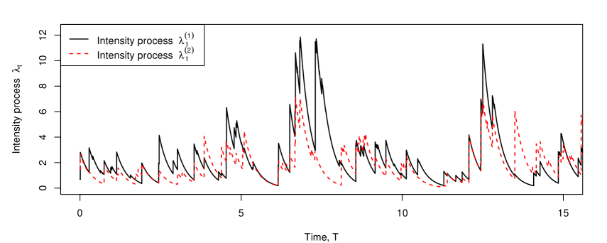
3.2. Joint Laplace Transform of ( λ T ( 1 ) , (\lambda_{T}^{\left(1\right)}, λ T ( 2 ) ) \lambda_{T}^{\left(2\right)})
Based on (3.1), we can easily derive the joint Laplace transform for the
process ( λ T ( 1 ) , (\lambda_{T}^{\left(1\right)}, λ T ( 2 ) ) \lambda_{T}^{\left(2\right)}) θ = 1 , 𝜃 1 \theta=1, η = 1 , 𝜂 1 \eta=1, ν = 0 , 𝜈 0 \nu=0, ζ = 0 . 𝜁 0 \zeta=0. 𝒢 υ , 1 − 1 ( T ) superscript subscript 𝒢 𝜐 1
1 𝑇 \mathcal{G}_{\upsilon,1}^{-1}(T) ℋ γ , 1 − 1 ( T ) superscript subscript ℋ 𝛾 1
1 𝑇 \mathcal{H}_{\gamma,1}^{-1}(T)
Proposition 3.1. The conditional joint Laplace transform
for the process ( λ T ( 1 ) , λ T ( 2 ) ) superscript subscript 𝜆 𝑇 1 superscript subscript 𝜆 𝑇 2 \left(\lambda_{T}^{\left(1\right)},\lambda_{T}^{\left(2\right)}\right) given λ 0 ( 1 ) superscript subscript 𝜆 0 1 \lambda_{0}^{\left(1\right)} λ 0 ( 2 ) superscript subscript 𝜆 0 2 \lambda_{0}^{\left(2\right)}
t = 0 𝑡 0 t=0 is given by
E [ e − υ λ T ( 1 ) e − γ λ T ( 2 ) ∣ λ 0 ( 1 ) , λ 0 ( 2 ) ] 𝐸 delimited-[] conditional superscript 𝑒 𝜐 superscript subscript 𝜆 𝑇 1 superscript 𝑒 𝛾 superscript subscript 𝜆 𝑇 2 superscript subscript 𝜆 0 1 superscript subscript 𝜆 0 2
\displaystyle E\left[e^{-\upsilon\lambda_{T}^{\left(1\right)}}e^{-\gamma\lambda_{T}^{\left(2\right)}}\mid\lambda_{0}^{\left(1\right)},\lambda_{0}^{\left(2\right)}\right] (37)
= \displaystyle= exp { − 𝒢 υ , 1 − 1 ( T ) λ 0 ( 1 ) } exp { − ℋ γ , 1 − 1 ( T ) λ 0 ( 2 ) } superscript subscript 𝒢 𝜐 1
1 𝑇 superscript subscript 𝜆 0 1 superscript subscript ℋ 𝛾 1
1 𝑇 superscript subscript 𝜆 0 2 \displaystyle\exp\left\{-\mathcal{G}_{\upsilon,1}^{-1}(T)\text{ }\lambda_{0}^{\left(1\right)}\right\}\exp\left\{-\mathcal{H}_{\gamma,1}^{-1}(T)\text{ }\lambda_{0}^{\left(2\right)}\right\}
× exp [ − ρ ∫ 0 T [ 1 − f ∧ { 𝒢 υ , 1 − 1 ( τ ) , ℋ γ , 1 − 1 ( τ ) } ] 𝑑 τ ] absent 𝜌 superscript subscript 0 𝑇 delimited-[] 1 𝑓 superscript subscript 𝒢 𝜐 1
1 𝜏 superscript subscript ℋ 𝛾 1
1 𝜏 differential-d 𝜏 \displaystyle\times\exp\left[-\rho\int\limits_{0}^{T}\left[1-\overset{\wedge}{f}\left\{\mathcal{G}_{\upsilon,1}^{-1}(\tau),\mathcal{H}_{\gamma,1}^{-1}(\tau)\right\}\right]d\tau\right]
× exp [ − ∫ 𝒢 υ , 1 − 1 ( T ) υ { a ( 1 ) δ ( 1 ) u δ ( 1 ) u + g ∧ ( u ) − 1 } 𝑑 u ] absent superscript subscript superscript subscript 𝒢 𝜐 1
1 𝑇 𝜐 superscript 𝑎 1 superscript 𝛿 1 𝑢 superscript 𝛿 1 𝑢 𝑔 𝑢 1 differential-d 𝑢 \displaystyle\times\exp\left[-\int\limits_{\mathcal{G}_{\upsilon,1}^{-1}(T)}^{\upsilon}\left\{\frac{a^{\left(1\right)}\delta^{\left(1\right)}\text{ }u}{\delta^{\left(1\right)}\text{ }u+\overset{\wedge}{g}\left(u\right)-1}\right\}du\right]
× exp [ − ∫ ℋ γ , 1 − 1 ( T ) γ { a ( 2 ) δ ( 2 ) u δ ( 2 ) u + h ∧ ( u ) − 1 } d u ] , \TCItag 3.10 \displaystyle\times\exp\left[-\int\limits_{\mathcal{H}_{\gamma,1}^{-1}(T)}^{\gamma}\left\{\frac{a^{\left(2\right)}\delta^{\left(2\right)}\text{ }u}{\delta^{\left(2\right)}\text{ }u+\overset{\wedge}{h}\left(u\right)-1}\right\}du\right],\TCItag{3.10}
where
μ 1 G = ∫ 0 ∞ y d G ( y ) , 𝒢 υ , 1 ( Ψ 1 ) = : ∫ Ψ 1 υ [ 1 δ ( 1 ) u + g ∧ ( u ) − 1 ] d u , \mu_{1_{G}}=\int\limits_{0}^{\infty}\text{ }ydG(y)\text{, \ \ }\mathcal{G}_{\upsilon,1}(\Psi_{1})=:\int\limits_{\Psi_{1}}^{\upsilon}\left[\frac{1}{\delta^{\left(1\right)}\text{ }u+\overset{\wedge}{g}\left(u\right)-1}\right]du\text{,}
μ 1 H = ∫ 0 ∞ z d H ( z ) , ℋ γ , 1 ( Ψ 2 ) = : ∫ Ψ 2 γ [ 1 δ ( 2 ) u + h ∧ ( u ) − 1 ] d u , \mu_{1_{H}}=\int\limits_{0}^{\infty}zdH(z),\ \ \mathcal{H}_{\gamma,1}(\Psi_{2})=:\int\limits_{\Psi_{2}}^{\gamma}\left[\frac{1}{\delta^{\left(2\right)}\text{ }u+\overset{\wedge}{h}\left(u\right)-1}\right]du,
δ ( 1 ) > μ 1 G and δ ( 2 ) > μ 1 H . superscript 𝛿 1 subscript 𝜇 subscript 1 𝐺 and superscript 𝛿 2 subscript 𝜇 subscript 1 𝐻 . \delta^{\left(1\right)}>\mu_{1_{G}}\text{ \ {and \ }}\delta^{\left(2\right)}>\mu_{1_{H}}\text{.}
Remark 1 . (3.10) is the conditional joint Laplace transform of
the process ( λ T ( 1 ) , λ T ( 2 ) ) superscript subscript 𝜆 𝑇 1 superscript subscript 𝜆 𝑇 2 \left(\lambda_{T}^{\left(1\right)},\lambda_{T}^{\left(2\right)}\right) λ 0 ( 1 ) superscript subscript 𝜆 0 1 \lambda_{0}^{\left(1\right)} λ 0 ( 2 ) superscript subscript 𝜆 0 2 \lambda_{0}^{\left(2\right)} t = 0 , 𝑡 0 t=0, X ( 1 ) superscript 𝑋 1 X^{\left(1\right)} X ( 2 ) superscript 𝑋 2 X^{\left(2\right)} F ( x ( 1 ) , x ( 2 ) ) 𝐹 superscript 𝑥 1 superscript 𝑥 2 F\left(x^{\left(1\right)},x^{\left(2\right)}\right) ρ 𝜌 \rho λ T ( 1 ) superscript subscript 𝜆 𝑇 1 \lambda_{T}^{(1)} λ 0 ( 1 ) superscript subscript 𝜆 0 1 \lambda_{0}^{\left(1\right)} λ T ( 2 ) superscript subscript 𝜆 𝑇 2 \lambda_{T}^{(2)} λ 0 ( 2 ) , superscript subscript 𝜆 0 2 \lambda_{0}^{\left(2\right)},
E [ e − υ λ T ( 1 ) e − γ λ T ( 2 ) ∣ λ 0 ( 1 ) , λ 0 ( 2 ) ] ≠ E [ e − υ λ T ( 1 ) ∣ λ 0 ( 1 ) ] E [ e − γ λ T ( 2 ) ∣ λ 0 ( 2 ) ] . 𝐸 delimited-[] conditional superscript 𝑒 𝜐 superscript subscript 𝜆 𝑇 1 superscript 𝑒 𝛾 superscript subscript 𝜆 𝑇 2 superscript subscript 𝜆 0 1 superscript subscript 𝜆 0 2
𝐸 delimited-[] conditional superscript 𝑒 𝜐 superscript subscript 𝜆 𝑇 1 superscript subscript 𝜆 0 1 𝐸 delimited-[] conditional superscript 𝑒 𝛾 superscript subscript 𝜆 𝑇 2 superscript subscript 𝜆 0 2 E\left[e^{-\upsilon\lambda_{T}^{\left(1\right)}}e^{-\gamma\lambda_{T}^{\left(2\right)}}\mid\lambda_{0}^{\left(1\right)},\lambda_{0}^{\left(2\right)}\right]\neq E\left[e^{-\upsilon\lambda_{T}^{\left(1\right)}}\mid\lambda_{0}^{\left(1\right)}\right]\text{ }E\left[e^{-\gamma\lambda_{T}^{\left(2\right)}}\mid\lambda_{0}^{\left(2\right)}\right]. (3.11)
Proposition 3.2. The joint Laplace transform of the
asymptotic distribution of ( λ T ( 1 ) , λ T ( 2 ) ) superscript subscript 𝜆 𝑇 1 superscript subscript 𝜆 𝑇 2 \left(\lambda_{T}^{\left(1\right)},\lambda_{T}^{\left(2\right)}\right) is given by
lim T → ∞ E [ e − υ λ T ( 1 ) e − γ λ T ( 2 ) ∣ λ 0 ( 1 ) , λ 0 ( 2 ) ] → 𝑇 𝐸 delimited-[] conditional superscript 𝑒 𝜐 superscript subscript 𝜆 𝑇 1 superscript 𝑒 𝛾 superscript subscript 𝜆 𝑇 2 superscript subscript 𝜆 0 1 superscript subscript 𝜆 0 2
\displaystyle\underset{T\rightarrow\infty}{\lim}E\left[e^{-\upsilon\lambda_{T}^{\left(1\right)}}e^{-\gamma\lambda_{T}^{\left(2\right)}}\mid\lambda_{0}^{\left(1\right)},\lambda_{0}^{\left(2\right)}\right] = \displaystyle= exp [ − ρ ∫ 0 ∞ [ 1 − f ∧ { 𝒢 υ , 1 − 1 ( τ ) , ℋ γ , 1 − 1 ( τ ) } ] 𝑑 τ ] 𝜌 superscript subscript 0 delimited-[] 1 𝑓 superscript subscript 𝒢 𝜐 1
1 𝜏 superscript subscript ℋ 𝛾 1
1 𝜏 differential-d 𝜏 \displaystyle\exp\left[-\rho\int\limits_{0}^{\infty}\left[1-\overset{\wedge}{f}\left\{\mathcal{G}_{\upsilon,1}^{-1}(\tau),\mathcal{H}_{\gamma,1}^{-1}(\tau)\right\}\right]d\tau\right] (38)
× exp [ − ∫ 0 υ { a ( 1 ) δ ( 1 ) u δ ( 1 ) u + g ∧ ( u ) − 1 } 𝑑 u ] absent superscript subscript 0 𝜐 superscript 𝑎 1 superscript 𝛿 1 𝑢 superscript 𝛿 1 𝑢 𝑔 𝑢 1 differential-d 𝑢 \displaystyle\times\exp\left[-\int\limits_{0}^{\upsilon}\left\{\frac{a^{\left(1\right)}\delta^{\left(1\right)}\text{ }u}{\delta^{\left(1\right)}\text{ }u+\overset{\wedge}{g}\left(u\right)-1}\right\}du\right]
× exp [ − ∫ 0 γ { a ( 2 ) δ ( 2 ) u δ ( 2 ) u + h ∧ ( u ) − 1 } d u ] , \TCItag 3.12 \displaystyle\times\exp\left[-\int\limits_{0}^{\gamma}\left\{\frac{a^{\left(2\right)}\delta^{\left(2\right)}\text{ }u}{\delta^{\left(2\right)}\text{ }u+\overset{\wedge}{h}\left(u\right)-1}\right\}du\right],\TCItag{3.12}
where δ ( 1 ) > μ 1 G superscript 𝛿 1 subscript 𝜇 subscript 1 𝐺 \delta^{\left(1\right)}>\mu_{1_{G}} and δ ( 2 ) > μ 1 H superscript 𝛿 2 subscript 𝜇 subscript 1 𝐻 \delta^{\left(2\right)}>\mu_{1_{H}} .
Remark 2 . We can easily derive the Laplace transform of λ T ( 1 ) superscript subscript 𝜆 𝑇 1 \lambda_{T}^{\left(1\right)} λ T ( 2 ) superscript subscript 𝜆 𝑇 2 \lambda_{T}^{\left(2\right)} T 𝑇 T ρ = 0 𝜌 0 \rho=0 the
conditional Laplace transform of λ T ( d ) superscript subscript 𝜆 𝑇 𝑑 \lambda_{T}^{\left(d\right)} ( d = 1 , 2 ) 𝑑 1 2
(d=1,2) λ 0 ( d ) superscript subscript 𝜆 0 𝑑 \lambda_{0}^{\left(d\right)} t = 0 𝑡 0 t=0
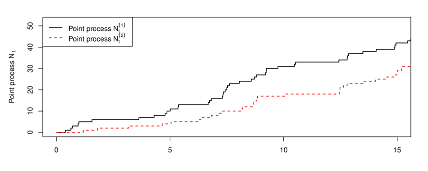
3.3 Joint Probability Generating Function of ( N T ( 1 ) , (N_{T}^{\left(1\right)}, N T ( 2 ) ) N_{T}^{\left(2\right)})
We derive the joint probability generating function for the
process ( N T ( 1 ) , (N_{T}^{\left(1\right)}, N T ( 2 ) ) N_{T}^{\left(2\right)}) T 𝑇 T
Theorem 3.2. The conditional joint probability generating
function for the process ( N T ( 1 ) , (N_{T}^{\left(1\right)}, N T ( 2 ) ) N_{T}^{\left(2\right)}) given λ 0 ( 1 ) superscript subscript 𝜆 0 1 \lambda_{0}^{\left(1\right)} λ 0 ( 2 ) , superscript subscript 𝜆 0 2 \lambda_{0}^{\left(2\right)}, N 0 ( 1 ) = 0 superscript subscript 𝑁 0 1 0 N_{0}^{\left(1\right)}=0
and N 0 ( 2 ) = 0 superscript subscript 𝑁 0 2 0 N_{0}^{\left(2\right)}=0 at time t = 0 𝑡 0 t=0 is
given by
E [ θ N T ( 1 ) η N T ( 2 ) ∣ λ 0 ( 1 ) , λ 0 ( 2 ) ] 𝐸 delimited-[] conditional superscript 𝜃 superscript subscript 𝑁 𝑇 1 superscript 𝜂 superscript subscript 𝑁 𝑇 2 superscript subscript 𝜆 0 1 superscript subscript 𝜆 0 2
\displaystyle E\left[\theta^{N_{T}^{\left(1\right)}}\eta^{N_{T}^{\left(2\right)}}\mid\lambda_{0}^{\left(1\right)},\text{ }\lambda_{0}^{\left(2\right)}\right] (39)
= \displaystyle= exp { − 𝒢 0 , θ − 1 ( T ) λ 0 ( 1 ) } exp { − ℋ 0 , η − 1 ( T ) λ 0 ( 2 ) } superscript subscript 𝒢 0 𝜃
1 𝑇 superscript subscript 𝜆 0 1 superscript subscript ℋ 0 𝜂
1 𝑇 superscript subscript 𝜆 0 2 \displaystyle\exp\left\{-\mathcal{G}_{0,\theta}^{-1}(T)\text{ }\lambda_{0}^{\left(1\right)}\right\}\exp\left\{-\mathcal{H}_{0,\eta}^{-1}(T)\lambda_{0}^{\left(2\right)}\right\}
× exp [ − ρ ∫ 0 T [ 1 − f ∧ { 𝒢 0 , θ − 1 ( τ ) , ℋ 0 , η − 1 ( τ ) } ] 𝑑 τ ] absent 𝜌 superscript subscript 0 𝑇 delimited-[] 1 𝑓 superscript subscript 𝒢 0 𝜃
1 𝜏 superscript subscript ℋ 0 𝜂
1 𝜏 differential-d 𝜏 \displaystyle\times\exp\left[-\rho\int\limits_{0}^{T}\left[1-\overset{\wedge}{f}\left\{\mathcal{G}_{0,\theta}^{-1}(\tau),\text{ }\mathcal{H}_{0,\eta}^{-1}(\tau)\right\}\right]d\tau\right]
× exp [ − ∫ 0 𝒢 0 , θ − 1 ( T ) { a ( 1 ) δ ( 1 ) u 1 − δ ( 1 ) u − θ g ∧ ( u ) } 𝑑 u ] absent superscript subscript 0 superscript subscript 𝒢 0 𝜃
1 𝑇 superscript 𝑎 1 superscript 𝛿 1 𝑢 1 superscript 𝛿 1 𝑢 𝜃 𝑔 𝑢 differential-d 𝑢 \displaystyle\times\exp\left[-\int\limits_{0}^{\mathcal{G}_{0,\theta}^{-1}(T)}\left\{\frac{a^{\left(1\right)}\delta^{\left(1\right)}\text{
}u}{1-\delta^{\left(1\right)}\text{ }u-\theta\overset{\wedge}{g}\left(u\right)}\right\}du\right]
× exp [ − ∫ 0 ℋ 0 , η − 1 ( T ) { a ( 2 ) δ ( 2 ) u 1 − δ ( 2 ) u − η h ∧ ( u ) } d u ] . \TCItag 3.13 \displaystyle\times\exp\left[-\int\limits_{0}^{\mathcal{H}_{0,\eta}^{-1}(T)}\left\{\frac{a^{\left(2\right)}\delta^{\left(2\right)}u}{1-\delta^{\left(2\right)}\text{ }u-\eta\overset{\wedge}{h}\left(u\right)}\right\}du\right].\TCItag{3.13}
Proof. By setting t = 0 , 𝑡 0 t=0, ν = 0 , 𝜈 0 \nu=0, ζ = 0 , 𝜁 0 \zeta=0, υ = 0 𝜐 0 \upsilon=0 γ = 0 𝛾 0 \gamma=0 N 0 ( 1 ) = 0 superscript subscript 𝑁 0 1 0 N_{0}^{\left(1\right)}=0 N 0 ( 2 ) = 0 superscript subscript 𝑁 0 2 0 N_{0}^{\left(2\right)}=0
E [ θ N T ( 1 ) η N T ( 2 ) ∣ ℑ 0 ] = e − B 1 ( 0 ) λ 0 ( 1 ) e − B 2 ( 0 ) λ 0 ( 2 ) e − C ( T ) , 𝐸 delimited-[] conditional superscript 𝜃 superscript subscript 𝑁 𝑇 1 superscript 𝜂 superscript subscript 𝑁 𝑇 2 subscript 0 superscript 𝑒 subscript 𝐵 1 0 superscript subscript 𝜆 0 1 superscript 𝑒 subscript 𝐵 2 0 superscript subscript 𝜆 0 2 superscript 𝑒 𝐶 𝑇 E\left[\theta^{N_{T}^{\left(1\right)}}\eta^{N_{T}^{\left(2\right)}}\mid\Im_{0}\right]=e^{-B_{1}(0)\lambda_{0}^{\left(1\right)}}e^{-B_{2}(0)\lambda_{0}^{\left(2\right)}}e^{-C(T)}, (3.14)
where B 1 ( 0 ) subscript 𝐵 1 0 B_{1}(0) non -linear ordinary
differential equation (ODE)
− B 1 ′ ( t ) + δ ( 1 ) B 1 ( t ) + θ g ∧ { B 1 ( t ) } − 1 = 0 superscript subscript 𝐵 1 ′ 𝑡 superscript 𝛿 1 subscript 𝐵 1 𝑡 𝜃 𝑔 subscript 𝐵 1 𝑡 1 0 -B_{1}^{\prime}(t)+\delta^{\left(1\right)}B_{1}(t)+\theta\text{ }\overset{\wedge}{g}\left\{B_{1}(t)\right\}-1=0 (3.15)
with boundary condition B 1 ( T ) = 0 subscript 𝐵 1 𝑇 0 B_{1}(T)=0 B 2 ( 0 ) subscript 𝐵 2 0 B_{2}(0) non -linear ODE
− B 2 ′ ( t ) + δ ( 2 ) B 2 ( t ) + η h ^ { B 2 ( t ) } − 1 = 0 superscript subscript 𝐵 2 ′ 𝑡 superscript 𝛿 2 subscript 𝐵 2 𝑡 𝜂 ^ ℎ subscript 𝐵 2 𝑡 1 0 -B_{2}^{\prime}(t)+\delta^{\left(2\right)}B_{2}(t)+\eta\text{ }\hat{h}\left\{B_{2}(t)\right\}-1=0 (3.16)
with boundary condition B 2 ( T ) = 0 . subscript 𝐵 2 𝑇 0 B_{2}(T)=0.
(3.15) can be solved, under the condition δ ( 1 ) > μ 1 G superscript 𝛿 1 subscript 𝜇 subscript 1 𝐺 \delta^{\left(1\right)}>\mu_{1_{G}}
(1) Set B 1 ( t ) = Ψ 1 ( T − t ) = Ψ 1 ( τ ) . subscript 𝐵 1 𝑡 subscript Ψ 1 𝑇 𝑡 subscript Ψ 1 𝜏 B_{1}(t)=\Psi_{1}(T-t)=\Psi_{1}(\tau).
d Ψ 1 ( τ ) d τ = 1 − δ ( 1 ) B 1 ( t ) − θ g ∧ { B 1 ( t ) } = 1 − δ 1 ( 1 ) Ψ 1 ( τ ) − θ g ∧ { Ψ 1 ( τ ) } = : f 1 ( Ψ 1 ) , 0 ≤ θ ≤ 1 \frac{d\Psi_{1}(\tau)}{d\tau}=1-\delta^{\left(1\right)}B_{1}(t)-\theta\overset{\wedge}{g}\left\{B_{1}(t)\right\}=1-\delta_{1}^{\left(1\right)}\Psi_{1}(\tau)-\theta\overset{\wedge}{g}\left\{\Psi_{1}(\tau)\right\}=:f_{1}(\Psi_{1}),\text{ \ \ }0\leq\theta\leq 1 (3.17)
with initial condition Ψ 1 ( 0 ) = 0 ; subscript Ψ 1 0 0 \Psi_{1}(0)=0; f 1 ( Ψ 1 ) subscript 𝑓 1 subscript Ψ 1 f_{1}(\Psi_{1})
(2) There is only one positive singular point, denoted by υ ∗ > 0 , superscript 𝜐 ∗ 0 \upsilon^{\ast}>0,
1 − δ ( 1 ) u − θ g ∧ ( u ) = 0 , 1 superscript 𝛿 1 𝑢 𝜃 𝑔 𝑢 0 1-\delta^{\left(1\right)}u-\theta\overset{\wedge}{g}\left(u\right)=0, (3.18)
at which the uniqueness of the solution of equation (3.18) is violated. This is because, for the case 0 < θ < 1 , 0 𝜃 1 0<\theta<1, f 1 ( Ψ 1 ) = 0 subscript 𝑓 1 subscript Ψ 1 0 f_{1}(\Psi_{1})=0
g ∧ ( u ) = 1 θ ( 1 − δ ( 1 ) u ) , 0 < θ < 1 . formulae-sequence 𝑔 𝑢 1 𝜃 1 superscript 𝛿 1 𝑢 0 𝜃 1 . \overset{\wedge}{g}\left(u\right)=\frac{1}{\theta}\left(1-\delta^{\left(1\right)}\text{ }u\right),\text{ \ }0<\theta<1\text{.} (3.19)
Note that the left-hand side of (3.19) is a convex function, hence it is
clear that there is only one positive solution to f 1 ( Ψ 1 ) subscript 𝑓 1 subscript Ψ 1 f_{1}(\Psi_{1}) θ = 0 𝜃 0 \theta=0
υ ∗ = 1 δ ( 1 ) > 0 . superscript 𝜐 ∗ 1 superscript 𝛿 1 0 \upsilon^{\ast}=\frac{1}{\delta^{\left(1\right)}}>0.
For both cases, we have
υ ∗ = 1 − θ g ∧ ( υ ∗ ) δ ( 1 ) ≥ 1 − θ δ ( 1 ) > 0 , superscript 𝜐 ∗ 1 𝜃 𝑔 superscript 𝜐 ∗ superscript 𝛿 1 1 𝜃 superscript 𝛿 1 0 \upsilon^{\ast}=\frac{1-\theta\overset{\wedge}{g}\left(\upsilon^{\ast}\right)}{\delta^{\left(1\right)}}\geq\frac{1-\theta}{\delta^{\left(1\right)}}>0,
hence, we have f 1 ( Ψ 1 ) > 0 subscript 𝑓 1 subscript Ψ 1 0 f_{1}(\Psi_{1})>0 0 ≤ Ψ 1 < υ ∗ 0 subscript Ψ 1 superscript 𝜐 ∗ 0\leq\Psi_{1}<\upsilon^{\ast} f 1 ( Ψ 1 ) < 0 subscript 𝑓 1 subscript Ψ 1 0 f_{1}(\Psi_{1})<0 Ψ 1 > υ ∗ subscript Ψ 1 superscript 𝜐 ∗ \Psi_{1}>\upsilon^{\ast}
(3) (3.17) can be written as
d Ψ 1 ( τ ) 1 − δ 1 ( 1 ) Ψ 1 ( τ ) − θ g ∧ { Ψ 1 ( τ ) } = d τ . 𝑑 subscript Ψ 1 𝜏 1 superscript subscript 𝛿 1 1 subscript Ψ 1 𝜏 𝜃 𝑔 subscript Ψ 1 𝜏 𝑑 𝜏 \frac{d\Psi_{1}(\tau)}{1-\delta_{1}^{\left(1\right)}\Psi_{1}(\tau)-\theta\overset{\wedge}{g}\left\{\Psi_{1}(\tau)\right\}}=d\tau.
Integrate both sides from time 0 0 τ , 𝜏 \tau,
∫ 0 Ψ 1 ( τ ) [ 1 1 − δ ( 1 ) u − θ g ∧ ( u ) ] 𝑑 u = τ , superscript subscript 0 subscript Ψ 1 𝜏 delimited-[] 1 1 superscript 𝛿 1 𝑢 𝜃 𝑔 𝑢 differential-d 𝑢 𝜏 \int\limits_{0}^{\Psi_{1}(\tau)}\left[\frac{1}{1-\delta^{\left(1\right)}u-\theta\overset{\wedge}{g}\left(u\right)}\right]du=\tau,
where 0 ≤ Ψ 1 ( τ ) < υ ∗ 0 subscript Ψ 1 𝜏 superscript 𝜐 ∗ 0\leq\Psi_{1}(\tau)<\upsilon^{\ast}
𝒢 0 , θ ( Ψ 1 ) = : ∫ 0 Ψ 1 ( τ ) [ 1 1 − δ ( 1 ) u − θ g ∧ ( u ) ] d u . \mathcal{G}_{0,\theta}(\Psi_{1})=:\int\limits_{0}^{\Psi_{1}(\tau)}\left[\frac{1}{1-\delta^{\left(1\right)}u-\theta\overset{\wedge}{g}\left(u\right)}\right]du.
Then we have
𝒢 0 , θ ( Ψ 1 ) = τ ( = T − t ) , subscript 𝒢 0 𝜃
subscript Ψ 1 annotated 𝜏 absent 𝑇 𝑡 \mathcal{G}_{0,\theta}(\Psi_{1})=\tau\text{ \ }(=T-t),
which is the time difference between T 𝑇 T t 𝑡 t Ψ 1 ( τ ) → 0 → subscript Ψ 1 𝜏 0 \Psi_{1}(\tau)\rightarrow 0 τ 𝜏 \tau → 0 → absent 0 \rightarrow 0 Ψ 1 ( τ ) → υ ∗ → subscript Ψ 1 𝜏 superscript 𝜐 ∗ \Psi_{1}(\tau)\rightarrow\upsilon^{\ast} τ 𝜏 \tau → ∞ → absent \rightarrow\infty u ∈ ( 0 , υ ∗ ] 𝑢 0 superscript 𝜐 ∗ u\in(0,\upsilon^{\ast}] Ψ 1 ( τ ) ≥ 0 subscript Ψ 1 𝜏 0 \Psi_{1}(\tau)\geq 0 𝒢 0 , θ ( Ψ 1 ) subscript 𝒢 0 𝜃
subscript Ψ 1 \mathcal{G}_{0,\theta}(\Psi_{1}) increasing function. Therefore
𝒢 0 , θ ( Ψ 1 ) = τ : [ 0 , υ ∗ ) → [ 0 , ∞ ) : subscript 𝒢 0 𝜃
subscript Ψ 1 𝜏 → 0 superscript 𝜐 ∗ 0 \mathcal{G}_{0,\theta}(\Psi_{1})=\tau:[0,\upsilon^{\ast})\rightarrow[0,\infty)
is a well defined function and it inverse function
𝒢 0 , θ − 1 ( τ ) = Ψ 1 : [ 0 , ∞ ) → [ 0 , υ ∗ ) : superscript subscript 𝒢 0 𝜃
1 𝜏 subscript Ψ 1 → 0 0 superscript 𝜐 ∗ \mathcal{G}_{0,\theta}^{-1}(\tau)=\Psi_{1}:[0,\infty)\rightarrow[0,\upsilon^{\ast})
exists.
(4) The unique solution is found by
Ψ 1 ( τ ) = Ψ 1 ( T − t ) = B 1 ( t ) = 𝒢 0 , θ − 1 ( τ ) = 𝒢 0 , θ − 1 ( T − t ) subscript Ψ 1 𝜏 subscript Ψ 1 𝑇 𝑡 subscript 𝐵 1 𝑡 superscript subscript 𝒢 0 𝜃
1 𝜏 superscript subscript 𝒢 0 𝜃
1 𝑇 𝑡 \Psi_{1}\left(\tau\right)=\Psi_{1}\left(T-t\right)=B_{1}(t)=\mathcal{G}_{0,\theta}^{-1}(\tau)=\mathcal{G}_{0,\theta}^{-1}(T-t)
and hence B 1 ( 0 ) subscript 𝐵 1 0 B_{1}(0)
B 1 ( 0 ) = Ψ 1 ( T ) = 𝒢 0 , θ − 1 ( T ) . subscript 𝐵 1 0 subscript Ψ 1 𝑇 superscript subscript 𝒢 0 𝜃
1 𝑇 B_{1}(0)=\Psi_{1}\left(T\right)=\mathcal{G}_{0,\theta}^{-1}(T).
(5) Similar to solving (3.15), under the condition δ ( 2 ) > μ 1 H , superscript 𝛿 2 subscript 𝜇 subscript 1 𝐻 \delta^{\left(2\right)}>\mu_{1_{H}},
Ψ 2 ( τ ) = Ψ 2 ( T − t ) = B 2 ( t ) = ℋ 0 , η − 1 ( τ ) = ℋ 0 , η − 1 ( T − t ) subscript Ψ 2 𝜏 subscript Ψ 2 𝑇 𝑡 subscript 𝐵 2 𝑡 superscript subscript ℋ 0 𝜂
1 𝜏 superscript subscript ℋ 0 𝜂
1 𝑇 𝑡 \Psi_{2}\left(\tau\right)=\Psi_{2}\left(T-t\right)=B_{2}(t)=\mathcal{H}_{0,\eta}^{-1}(\tau)=\mathcal{H}_{0,\eta}^{-1}(T-t)
and hence B 2 ( 0 ) subscript 𝐵 2 0 B_{2}(0)
B 2 ( 0 ) = Ψ 2 ( T ) = ℋ 0 , η − 1 ( T ) , subscript 𝐵 2 0 subscript Ψ 2 𝑇 superscript subscript ℋ 0 𝜂
1 𝑇 B_{2}(0)=\Psi_{2}\left(T\right)=\mathcal{H}_{0,\eta}^{-1}(T),
where
ℋ 0 , η ( Ψ 2 ) = ∫ 0 Ψ 2 ( τ ) [ 1 1 − δ ( 2 ) u − η h ∧ ( u ) ] 𝑑 u subscript ℋ 0 𝜂
subscript Ψ 2 superscript subscript 0 subscript Ψ 2 𝜏 delimited-[] 1 1 superscript 𝛿 2 𝑢 𝜂 ℎ 𝑢 differential-d 𝑢 \mathcal{H}_{0,\eta}(\Psi_{2})=\int\limits_{0}^{\Psi_{2}(\tau)}\left[\frac{1}{1-\delta^{\left(2\right)}\text{ }u-\eta\overset{\wedge}{h}\left(u\right)}\right]du
is also a strictly increasing function: the integrand is positive
in the domain u ∈ ( 0 , γ ∗ ] 𝑢 0 superscript 𝛾 ∗ u\in(0,\gamma^{\ast}] Ψ 2 ( τ ) ≥ 0 subscript Ψ 2 𝜏 0 \Psi_{2}(\tau)\geq 0
ℋ 0 , η ( Ψ 2 ) = τ : [ 0 , γ ∗ ) → [ 0 , ∞ ) : subscript ℋ 0 𝜂
subscript Ψ 2 𝜏 → 0 superscript 𝛾 ∗ 0 \mathcal{H}_{0,\eta}(\Psi_{2})=\tau:[0,\gamma^{\ast})\rightarrow[0,\infty)
is a well defined function and it inverse function
ℋ 0 , η − 1 ( τ ) = Ψ 2 : [ 0 , ∞ ) → [ 0 , γ ∗ ) : superscript subscript ℋ 0 𝜂
1 𝜏 subscript Ψ 2 → 0 0 superscript 𝛾 ∗ \mathcal{H}_{0,\eta}^{-1}(\tau)=\Psi_{2}:[0,\infty)\rightarrow[0,\gamma^{\ast})
exists.
(6) C ( T ) 𝐶 𝑇 C(T)
C ( T ) = ρ ∫ 0 T [ 1 − f ∧ { 𝒢 0 , θ − 1 ( τ ) , ℋ 0 , η − 1 ( τ ) } ] 𝑑 τ + δ ( 1 ) a ( 1 ) ∫ 0 T 𝒢 0 , θ − 1 ( τ ) 𝑑 τ + δ ( 2 ) a ( 2 ) ∫ 0 T ℋ 0 , η − 1 ( τ ) 𝑑 τ , 𝐶 𝑇 𝜌 superscript subscript 0 𝑇 delimited-[] 1 𝑓 superscript subscript 𝒢 0 𝜃
1 𝜏 superscript subscript ℋ 0 𝜂
1 𝜏 differential-d 𝜏 superscript 𝛿 1 superscript 𝑎 1 superscript subscript 0 𝑇 superscript subscript 𝒢 0 𝜃
1 𝜏 differential-d 𝜏 superscript 𝛿 2 superscript 𝑎 2 superscript subscript 0 𝑇 superscript subscript ℋ 0 𝜂
1 𝜏 differential-d 𝜏 C(T)=\rho\int\limits_{0}^{T}\left[1-\overset{\wedge}{f}\left\{\mathcal{G}_{0,\theta}^{-1}(\tau),\text{ }\mathcal{H}_{0,\eta}^{-1}(\tau)\right\}\right]d\tau+\delta^{\left(1\right)}a^{\left(1\right)}\int\limits_{0}^{T}\mathcal{G}_{0,\theta}^{-1}(\tau)d\tau+\delta^{\left(2\right)}a^{\left(2\right)}\int\limits_{0}^{T}\mathcal{H}_{0,\eta}^{-1}(\tau)d\tau,
and by the change of variable 𝒢 0 , θ − 1 ( τ ) = u , superscript subscript 𝒢 0 𝜃
1 𝜏 𝑢 \mathcal{G}_{0,\theta}^{-1}(\tau)=u, τ = 𝒢 0 , θ ( u ) 𝜏 subscript 𝒢 0 𝜃
𝑢 \tau=\mathcal{G}_{0,\theta}(u) → → \rightarrow d τ = ∂ 𝒢 0 , θ ( u ) ∂ u d u 𝑑 𝜏 subscript 𝒢 0 𝜃
𝑢 𝑢 𝑑 𝑢 d\tau=\frac{\partial\mathcal{G}_{0,\theta}(u)}{\partial u}du
∫ 0 T 𝒢 0 , θ − 1 ( τ ) 𝑑 τ = ∫ 0 𝒢 0 , θ − 1 ( T ) u 1 − δ ( 1 ) u − θ g ∧ ( u ) 𝑑 u superscript subscript 0 𝑇 superscript subscript 𝒢 0 𝜃
1 𝜏 differential-d 𝜏 superscript subscript 0 superscript subscript 𝒢 0 𝜃
1 𝑇 𝑢 1 superscript 𝛿 1 𝑢 𝜃 𝑔 𝑢 differential-d 𝑢 \int\limits_{0}^{T}\mathcal{G}_{0,\theta}^{-1}(\tau)d\tau=\int\limits_{0}^{\mathcal{G}_{0,\theta}^{-1}(T)}\frac{u}{1-\delta^{\left(1\right)}\text{ }u-\theta\overset{\wedge}{g}\left(u\right)}du
and similarly, ℋ 0 , η − 1 ( τ ) = u , superscript subscript ℋ 0 𝜂
1 𝜏 𝑢 \mathcal{H}_{0,\eta}^{-1}(\tau)=u, τ = ℋ 0 , η ( u ) 𝜏 subscript ℋ 0 𝜂
𝑢 \tau=\mathcal{H}_{0,\eta}(u) → → \rightarrow d τ = ∂ ℋ 0 , η ( u ) ∂ u d u 𝑑 𝜏 subscript ℋ 0 𝜂
𝑢 𝑢 𝑑 𝑢 d\tau=\frac{\partial\mathcal{H}_{0,\eta}(u)}{\partial u}du
∫ 0 T ℋ 0 , η − 1 ( τ ) 𝑑 τ = ∫ 0 ℋ 0 , η − 1 ( T ) u 1 − δ ( 2 ) u − η h ∧ ( u ) 𝑑 u superscript subscript 0 𝑇 superscript subscript ℋ 0 𝜂
1 𝜏 differential-d 𝜏 superscript subscript 0 superscript subscript ℋ 0 𝜂
1 𝑇 𝑢 1 superscript 𝛿 2 𝑢 𝜂 ℎ 𝑢 differential-d 𝑢 \int\limits_{0}^{T}\mathcal{H}_{0,\eta}^{-1}(\tau)d\tau=\int\limits_{0}^{\mathcal{H}_{0,\eta}^{-1}(T)}\frac{u}{1-\delta^{\left(2\right)}\text{ }u-\eta\overset{\wedge}{h}\left(u\right)}du
(7) Finally, substitute B 1 ( 0 ) , subscript 𝐵 1 0 B_{1}(0), B 2 ( 0 ) subscript 𝐵 2 0 B_{2}(0) C ( T ) 𝐶 𝑇 C(T)
Remark 3 . We can easily derive the Laplace transform of N T ( 1 ) superscript subscript 𝑁 𝑇 1 N_{T}^{\left(1\right)} N T ( 2 ) superscript subscript 𝑁 𝑇 2 N_{T}^{\left(2\right)} T 𝑇 T ρ = 0 𝜌 0 \rho=0 the
conditional Laplace transform of N T ( d ) superscript subscript 𝑁 𝑇 𝑑 N_{T}^{\left(d\right)} ( d = 1 , 2 ) 𝑑 1 2
(d=1,2) λ 0 ( d ) superscript subscript 𝜆 0 𝑑 \lambda_{0}^{\left(d\right)} t = 0 𝑡 0 t=0
3.4. Joint Laplace Transform of ( L T ( 1 ) , (L_{T}^{\left(1\right)}, L T ( 2 ) ) L_{T}^{\left(2\right)})
To derive the joint Laplace transform of the process ( L T ( 1 ) , (L_{T}^{\left(1\right)}, L T ( 2 ) ) L_{T}^{\left(2\right)}) T 𝑇 T ( λ T ( 1 ) , (\lambda_{T}^{\left(1\right)}, λ T ( 2 ) ) \lambda_{T}^{\left(2\right)}) ( L T ( 1 ) , (L_{T}^{\left(1\right)}, L T ( 2 ) ) L_{T}^{\left(2\right)})
Theorem 3.3 The conditional joint Laplace transform ,
probability generating function of the process ( λ T ( 1 ) , (\lambda_{T}^{\left(1\right)}, λ T ( 2 ) ) \lambda_{T}^{\left(2\right)}) and the
compound point process ( L T ( 1 ) , (L_{T}^{\left(1\right)}, L T ( 2 ) ) L_{T}^{\left(2\right)}) given λ 0 ( 1 ) superscript subscript 𝜆 0 1 \lambda_{0}^{\left(1\right)} λ 0 ( 2 ) superscript subscript 𝜆 0 2 \lambda_{0}^{\left(2\right)} , and L 0 ( 1 ) = 0 superscript subscript 𝐿 0 1 0 L_{0}^{\left(1\right)}=0 and L 0 ( 2 ) = 0 superscript subscript 𝐿 0 2 0 L_{0}^{\left(2\right)}=0 at time t = 0 𝑡 0 t=0 is given by
E [ e − ν L T ( 1 ) e − ζ L T ( 2 ) × e − υ λ T ( 1 ) e − γ λ T ( 2 ) ∣ λ 0 ( 1 ) , λ 0 ( 2 ) ] 𝐸 delimited-[] conditional superscript 𝑒 𝜈 superscript subscript 𝐿 𝑇 1 superscript 𝑒 𝜁 superscript subscript 𝐿 𝑇 2 superscript 𝑒 𝜐 superscript subscript 𝜆 𝑇 1 superscript 𝑒 𝛾 superscript subscript 𝜆 𝑇 2 superscript subscript 𝜆 0 1 superscript subscript 𝜆 0 2
\displaystyle E\left[e^{-\nu L_{T}^{\left(1\right)}}e^{-\zeta L_{T}^{\left(2\right)}}\times e^{-\upsilon\lambda_{T}^{\left(1\right)}}e^{-\gamma\lambda_{T}^{\left(2\right)}}\mid\lambda_{0}^{\left(1\right)},\text{ }\lambda_{0}^{\left(2\right)}\right] (40)
= \displaystyle= exp { − 𝒢 υ , ν − 1 ( T ) λ 0 ( 1 ) } exp { − ℋ γ , ζ − 1 ( T ) λ 0 ( 2 ) } superscript subscript 𝒢 𝜐 𝜈
1 𝑇 superscript subscript 𝜆 0 1 superscript subscript ℋ 𝛾 𝜁
1 𝑇 superscript subscript 𝜆 0 2 \displaystyle\exp\left\{-\mathcal{G}_{\upsilon,\nu}^{-1}(T)\text{ }\lambda_{0}^{\left(1\right)}\right\}\exp\left\{-\mathcal{H}_{\gamma,\zeta}^{-1}(T)\text{ }\lambda_{0}^{\left(2\right)}\right\}
× exp [ − ρ ∫ 0 T [ 1 − f ∧ { 𝒢 υ , ν − 1 ( τ ) , ℋ γ , ζ − 1 ( τ ) } ] 𝑑 τ ] absent 𝜌 superscript subscript 0 𝑇 delimited-[] 1 𝑓 superscript subscript 𝒢 𝜐 𝜈
1 𝜏 superscript subscript ℋ 𝛾 𝜁
1 𝜏 differential-d 𝜏 \displaystyle\times\exp\left[-\rho\int\limits_{0}^{T}\left[1-\overset{\wedge}{f}\left\{\mathcal{G}_{\upsilon,\nu}^{-1}(\tau),\mathcal{H}_{\gamma,\zeta}^{-1}(\tau)\right\}\right]d\tau\right]
× exp [ − ∫ 𝒢 υ , ν − 1 ( T ) υ { a ( 1 ) δ ( 1 ) u δ ( 1 ) u + j ∧ ( ν ) g ∧ ( u ) − 1 } 𝑑 u ] absent superscript subscript superscript subscript 𝒢 𝜐 𝜈
1 𝑇 𝜐 superscript 𝑎 1 superscript 𝛿 1 𝑢 superscript 𝛿 1 𝑢 𝑗 𝜈 𝑔 𝑢 1 differential-d 𝑢 \displaystyle\times\exp\left[-\int\limits_{\mathcal{G}_{\upsilon,\nu}^{-1}(T)}^{\upsilon}\left\{\frac{a^{\left(1\right)}\delta^{\left(1\right)}\text{ }u}{\delta^{\left(1\right)}\text{ }u+\text{ }\overset{\wedge}{j}\left(\nu\right)\overset{\wedge}{g}\left(u\right)-1}\right\}du\right]
× exp [ − ∫ ℋ γ , ζ − 1 ( T ) γ { a ( 2 ) δ ( 2 ) u δ ( 2 ) u + k ∧ ( ξ ) h ∧ ( u ) − 1 } 𝑑 u ] , absent superscript subscript superscript subscript ℋ 𝛾 𝜁
1 𝑇 𝛾 superscript 𝑎 2 superscript 𝛿 2 𝑢 superscript 𝛿 2 𝑢 𝑘 𝜉 ℎ 𝑢 1 differential-d 𝑢 \displaystyle\times\exp\left[-\int\limits_{\mathcal{H}_{\gamma,\zeta}^{-1}(T)}^{\gamma}\left\{\frac{a^{\left(2\right)}\delta^{\left(2\right)}\text{ }u}{\delta^{\left(2\right)}\text{ }u+\text{ }\overset{\wedge}{k}\left(\xi\right)\overset{\wedge}{h}\left(u\right)-1}\right\}du\right],
\TCItag 3.20 \TCItag 3.20 \displaystyle\TCItag{3.20}
μ 1 G = ∫ 0 ∞ y 𝑑 G ( y ) , 𝒢 υ , ν ( Ψ 1 ) = ∫ Ψ 1 υ [ 1 δ ( 1 ) u + j ∧ ( ν ) g ∧ ( u ) − 1 ] 𝑑 u , subscript 𝜇 subscript 1 𝐺 superscript subscript 0 𝑦 differential-d 𝐺 𝑦 , subscript 𝒢 𝜐 𝜈
subscript Ψ 1 superscript subscript subscript Ψ 1 𝜐 delimited-[] 1 superscript 𝛿 1 𝑢 𝑗 𝜈 𝑔 𝑢 1 differential-d 𝑢 , \mu_{1_{G}}=\int\limits_{0}^{\infty}\text{ }ydG(y)\text{, \ \ }\mathcal{G}_{\upsilon,\nu}(\Psi_{1})=\int\limits_{\Psi_{1}}^{\upsilon}\left[\frac{1}{\delta^{\left(1\right)}\text{ }u+\text{ }\overset{\wedge}{j}\left(\nu\right)\overset{\wedge}{g}\left(u\right)-1}\right]du\text{,}
μ 1 H = ∫ 0 ∞ z 𝑑 H ( z ) , ℋ γ , ζ ( Ψ 2 ) = ∫ Ψ 2 γ [ 1 δ ( 2 ) u + k ∧ ( ζ ) h ∧ ( u ) − 1 ] 𝑑 u , subscript 𝜇 subscript 1 𝐻 superscript subscript 0 𝑧 differential-d 𝐻 𝑧 , subscript ℋ 𝛾 𝜁
subscript Ψ 2 superscript subscript subscript Ψ 2 𝛾 delimited-[] 1 superscript 𝛿 2 𝑢 𝑘 𝜁 ℎ 𝑢 1 differential-d 𝑢 \mu_{1_{H}}=\int\limits_{0}^{\infty}\text{ }zdH(z)\text{, \ \ }\mathcal{H}_{\gamma,\zeta}(\Psi_{2})=\int\limits_{\Psi_{2}}^{\gamma}\left[\frac{1}{\delta^{\left(2\right)}\text{ }u+\text{ }\overset{\wedge}{k}\left(\zeta\right)\overset{\wedge}{h}\left(u\right)-1}\right]du,
δ ( 1 ) > j ∧ ( ν ) μ 1 G and δ ( 2 ) > k ∧ ( ξ ) μ 1 H . superscript 𝛿 1 𝑗 𝜈 subscript 𝜇 subscript 1 𝐺 and superscript 𝛿 2 𝑘 𝜉 subscript 𝜇 subscript 1 𝐻 . \delta^{\left(1\right)}>\text{ }\overset{\wedge}{j}\left(\nu\right)\mu_{1_{G}}\text{ \ {and \ }}\delta^{\left(2\right)}>\text{ }\overset{\wedge}{k}\left(\xi\right)\mu_{1_{H}}\text{.}
Proof. By setting t = 0 , 𝑡 0 t=0, θ = 1 , 𝜃 1 \theta=1, η = 1 , 𝜂 1 \eta=1,
E [ e − ν L T ( 1 ) e − ζ L T ( 2 ) e − υ λ T ( 1 ) e − γ λ T ( 2 ) ∣ ℑ 0 ] = e − B 1 ( 0 ) λ 0 ( 1 ) e − B 2 ( 0 ) λ 0 ( 2 ) e − C ( T ) , 𝐸 delimited-[] conditional superscript 𝑒 𝜈 superscript subscript 𝐿 𝑇 1 superscript 𝑒 𝜁 superscript subscript 𝐿 𝑇 2 superscript 𝑒 𝜐 superscript subscript 𝜆 𝑇 1 superscript 𝑒 𝛾 superscript subscript 𝜆 𝑇 2 subscript 0 superscript 𝑒 subscript 𝐵 1 0 superscript subscript 𝜆 0 1 superscript 𝑒 subscript 𝐵 2 0 superscript subscript 𝜆 0 2 superscript 𝑒 𝐶 𝑇 E\left[e^{-\nu L_{T}^{\left(1\right)}}e^{-\zeta L_{T}^{\left(2\right)}}\text{ }e^{-\upsilon\lambda_{T}^{\left(1\right)}}e^{-\gamma\lambda_{T}^{\left(2\right)}}\mid\Im_{0}\right]=e^{-B_{1}(0)\lambda_{0}^{\left(1\right)}}e^{-B_{2}(0)\lambda_{0}^{\left(2\right)}}e^{-C(T)}, (3.21)
where B 1 ( 0 ) subscript 𝐵 1 0 B_{1}(0) non -linear ordinary
differential equation (ODE)
− B 1 ′ ( t ) + δ ( 1 ) B 1 ( t ) + g ∧ { B 1 ( t ) } j ∧ ( ν ) − 1 = 0 superscript subscript 𝐵 1 ′ 𝑡 superscript 𝛿 1 subscript 𝐵 1 𝑡 𝑔 subscript 𝐵 1 𝑡 𝑗 𝜈 1 0 -B_{1}^{\prime}\left(t\right)+\delta^{\left(1\right)}B_{1}\left(t\right)+\overset{\wedge}{g}\left\{B_{1}\left(t\right)\right\}\text{ }\overset{\wedge}{j}\left(\nu\right)-1=0 (3.22)
with boundary condition B 1 ( T ) = υ subscript 𝐵 1 𝑇 𝜐 B_{1}\left(T\right)=\upsilon B 2 ( 0 ) subscript 𝐵 2 0 B_{2}(0) non -linear ODE
− B 2 ′ ( t ) + δ ( 2 ) B 2 ( t ) + h ∧ { B 2 ( t ) } k ∧ ( ζ ) − 1 = 0 superscript subscript 𝐵 2 ′ 𝑡 superscript 𝛿 2 subscript 𝐵 2 𝑡 ℎ subscript 𝐵 2 𝑡 𝑘 𝜁 1 0 -B_{2}^{\prime}\left(t\right)+\delta^{\left(2\right)}B_{2}\left(t\right)+\overset{\wedge}{h}\left\{B_{2}\left(t\right)\right\}\text{ }\overset{\wedge}{k}\left(\zeta\right)-1=0 (3.23)
with boundary condition B 2 ( T ) = γ . subscript 𝐵 2 𝑇 𝛾 B_{2}(T)=\gamma.
(3.22) can be solved, under the condition δ ( 1 ) > superscript 𝛿 1 absent \delta^{\left(1\right)}> j ∧ ( ν ) 𝑗 𝜈 \overset{\wedge}{j}\left(\nu\right) μ 1 G subscript 𝜇 subscript 1 𝐺 \mu_{1_{G}}
(1) Let us set B 1 ( t ) = Ψ 1 ( T − t ) = Ψ 1 ( τ ) . subscript 𝐵 1 𝑡 subscript Ψ 1 𝑇 𝑡 subscript Ψ 1 𝜏 B_{1}(t)=\Psi_{1}(T-t)=\Psi_{1}(\tau).
d Ψ 1 ( τ ) d τ = 1 − δ ( 1 ) B 1 ( t ) − g ∧ { B 1 ( t ) } j ∧ ( ν ) = 1 − δ ( 1 ) Ψ 1 ( τ ) − g ∧ { Ψ 1 ( τ ) } j ∧ ( ν ) = : f 2 ( Ψ 1 ) \frac{d\Psi_{1}(\tau)}{d\tau}=1-\delta^{\left(1\right)}B_{1}(t)-\overset{\wedge}{g}\left\{B_{1}(t)\right\}\overset{\wedge}{j}\left(\nu\right)=1-\delta^{\left(1\right)}\Psi_{1}(\tau)-\overset{\wedge}{g}\left\{\Psi_{1}(\tau)\right\}\overset{\wedge}{j}\left(\nu\right)=:f_{2}(\Psi_{1}) (3.24)
with initial condition Ψ 1 ( 0 ) = υ ; subscript Ψ 1 0 𝜐 \Psi_{1}(0)=\upsilon; f 2 ( Ψ 1 ) subscript 𝑓 2 subscript Ψ 1 f_{2}(\Psi_{1})
(2) For ν = 0 𝜈 0 \nu=0
f 2 ( Ψ 1 ) = 1 − δ ( 1 ) Ψ 1 ( τ ) − g ∧ { Ψ 1 ( τ ) } subscript 𝑓 2 subscript Ψ 1 1 superscript 𝛿 1 subscript Ψ 1 𝜏 𝑔 subscript Ψ 1 𝜏 f_{2}(\Psi_{1})=1-\delta^{\left(1\right)}\Psi_{1}(\tau)-\overset{\wedge}{g}\left\{\Psi_{1}(\tau)\right\}
and its unique solution is found by Ψ 1 ( τ ) = 𝒢 υ , 1 − 1 ( τ ) , subscript Ψ 1 𝜏 superscript subscript 𝒢 𝜐 1
1 𝜏 \Psi_{1}(\tau)=\mathcal{G}_{\upsilon,1}^{-1}(\tau),
Under the condition of δ ( 1 ) > superscript 𝛿 1 absent \delta^{\left(1\right)}> j ∧ ( ν ) 𝑗 𝜈 \overset{\wedge}{j}\left(\nu\right) μ 1 G subscript 𝜇 subscript 1 𝐺 \mu_{1_{G}}
∂ f 2 ( Ψ 1 ) ∂ Ψ 1 = j ∧ ( ν ) ∫ 0 ∞ y e − Ψ 1 y 𝑑 G ( y ) − δ ( 1 ) ≤ j ∧ ( ν ) ∫ 0 ∞ y 𝑑 G ( y ) − δ ( 1 ) = j ∧ ( ν ) μ 1 G − δ ( 1 ) < 0 , for Ψ 1 ≥ 0 , formulae-sequence subscript 𝑓 2 subscript Ψ 1 subscript Ψ 1 𝑗 𝜈 superscript subscript 0 𝑦 superscript 𝑒 subscript Ψ 1 𝑦 differential-d 𝐺 𝑦 superscript 𝛿 1 𝑗 𝜈 superscript subscript 0 𝑦 differential-d 𝐺 𝑦 superscript 𝛿 1 𝑗 𝜈 subscript 𝜇 subscript 1 𝐺 superscript 𝛿 1 0 for subscript Ψ 1 0 \frac{\partial f_{2}(\Psi_{1})}{\partial\Psi_{1}}=\overset{\wedge}{j}\left(\nu\right)\int\limits_{0}^{\infty}ye^{-\Psi_{1}\text{ }y\text{ }}dG(y)-\delta^{\left(1\right)}\text{ }\leq\text{ }\overset{\wedge}{j}\left(\nu\right)\int\limits_{0}^{\infty}\text{ }ydG(y)-\delta^{\left(1\right)}=\text{ }\overset{\wedge}{j}\left(\nu\right)\mu_{1_{G}}-\delta^{\left(1\right)}<0,\text{ \ for }\Psi_{1}\geq 0,
then f 2 ( Ψ 1 ) < 0 subscript 𝑓 2 subscript Ψ 1 0 f_{2}(\Psi_{1})<0 Ψ 1 > 0 subscript Ψ 1 0 \Psi_{1}>0
(3) (3.24) can be written as
d Ψ 1 ( τ ) δ ( 1 ) Ψ 1 ( τ ) − j ∧ ( ν ) g ∧ { Ψ 1 ( τ ) } − 1 = − d τ . 𝑑 subscript Ψ 1 𝜏 superscript 𝛿 1 subscript Ψ 1 𝜏 𝑗 𝜈 𝑔 subscript Ψ 1 𝜏 1 𝑑 𝜏 \frac{d\Psi_{1}(\tau)}{\delta^{\left(1\right)}\Psi_{1}(\tau)-\text{ }\overset{\wedge}{j}\left(\nu\right)\overset{\wedge}{g}\left\{\Psi_{1}(\tau)\right\}-1}=-d\tau.
Integrate both sides from time 0 to τ 𝜏 \tau Ψ 1 ( 0 ) = υ > 0 , subscript Ψ 1 0 𝜐 0 \Psi_{1}(0)=\upsilon>0,
∫ Ψ 1 υ [ 1 δ ( 1 ) u + j ∧ ( ν ) g ∧ ( u ) − 1 ] 𝑑 u = τ , superscript subscript subscript Ψ 1 𝜐 delimited-[] 1 superscript 𝛿 1 𝑢 𝑗 𝜈 𝑔 𝑢 1 differential-d 𝑢 𝜏 \int\limits_{\Psi_{1}}^{\upsilon}\left[\frac{1}{\delta^{\left(1\right)}\text{ }u+\text{ }\overset{\wedge}{j}\left(\nu\right)\overset{\wedge}{g}\left(u\right)-1}\right]du=\tau,
where Ψ 1 ≥ 0 . subscript Ψ 1 0 \Psi_{1}\geq 0.
𝒢 υ , ν ( Ψ 1 ) = : ∫ Ψ 1 υ [ 1 δ ( 1 ) u + j ∧ ( ν ) g ∧ ( u ) − 1 ] d u . \mathcal{G}_{\upsilon,\nu}(\Psi_{1})=:\int\limits_{\Psi_{1}}^{\upsilon}\left[\frac{1}{\delta^{\left(1\right)}\text{ }u+\text{ }\overset{\wedge}{j}\left(\nu\right)\overset{\wedge}{g}\left(u\right)-1}\right]du.
Then we have
𝒢 υ , ν ( Ψ 1 ) = τ ( = T − t ) , subscript 𝒢 𝜐 𝜈
subscript Ψ 1 annotated 𝜏 absent 𝑇 𝑡 \mathcal{G}_{\upsilon,\nu}(\Psi_{1})=\tau\text{ }(=T-t),
which is the time difference between T 𝑇 T t 𝑡 t Ψ 1 → υ → subscript Ψ 1 𝜐 \Psi_{1}\rightarrow\upsilon τ 𝜏 \tau ( = T − t ) → 0 . (=T-t)\rightarrow 0.
(4) As δ ( 1 ) − limit-from superscript 𝛿 1 \delta^{\left(1\right)}- j ∧ ( ν ) μ 1 G > 0 𝑗 𝜈 subscript 𝜇 subscript 1 𝐺 0 \overset{\wedge}{j}\left(\nu\right)\mu_{1_{G}}>0
∫ 0 υ [ 1 δ ( 1 ) u + j ∧ ( ν ) g ∧ ( u ) − 1 ] 𝑑 u = ∞ superscript subscript 0 𝜐 delimited-[] 1 superscript 𝛿 1 𝑢 𝑗 𝜈 𝑔 𝑢 1 differential-d 𝑢 \int\limits_{0}^{\upsilon}\left[\frac{1}{\delta^{\left(1\right)}\text{ }u+\text{ }\overset{\wedge}{j}\left(\nu\right)\overset{\wedge}{g}\left(u\right)-1}\right]du=\infty
so Ψ 1 → 0 → subscript Ψ 1 0 \Psi_{1}\rightarrow 0 τ → ∞ . → 𝜏 \tau\rightarrow\infty. u ∈ ( 0 , υ ] 𝑢 0 𝜐 u\in(0,\upsilon] Ψ 1 ≤ υ subscript Ψ 1 𝜐 \Psi_{1}\leq\upsilon 𝒢 υ , ν ( Ψ 1 ) subscript 𝒢 𝜐 𝜈
subscript Ψ 1 \mathcal{G}_{\upsilon,\nu}(\Psi_{1}) decreasing function. Therefore
𝒢 υ , ν ( Ψ 1 ) = τ : ( 0 , υ ] → [ 0 , ∞ ) : subscript 𝒢 𝜐 𝜈
subscript Ψ 1 𝜏 → 0 𝜐 0 \mathcal{G}_{\upsilon,\nu}(\Psi_{1})=\tau:(0,\upsilon]\rightarrow[0,\infty)
is a well defined (monotone) function and its inverse function
𝒢 υ , ν − 1 ( τ ) = Ψ 1 : [ 0 , ∞ ) → ( 0 , υ ] : superscript subscript 𝒢 𝜐 𝜈
1 𝜏 subscript Ψ 1 → 0 0 𝜐 \mathcal{G}_{\upsilon,\nu}^{-1}(\tau)=\Psi_{1}:[0,\infty)\rightarrow(0,\upsilon]
(5) The unique solution is found by
Ψ 1 ( τ ) = Ψ 1 ( T − t ) = B 1 ( t ) = 𝒢 υ , ν − 1 ( τ ) = 𝒢 υ , ν − 1 ( T − t ) subscript Ψ 1 𝜏 subscript Ψ 1 𝑇 𝑡 subscript 𝐵 1 𝑡 superscript subscript 𝒢 𝜐 𝜈
1 𝜏 superscript subscript 𝒢 𝜐 𝜈
1 𝑇 𝑡 \Psi_{1}\left(\tau\right)=\Psi_{1}\left(T-t\right)=B_{1}(t)=\mathcal{G}_{\upsilon,\nu}^{-1}(\tau)=\mathcal{G}_{\upsilon,\nu}^{-1}(T-t)
and hence B 1 ( 0 ) subscript 𝐵 1 0 B_{1}(0)
B 1 ( 0 ) = Ψ 1 ( T ) = 𝒢 υ , ν − 1 ( T ) . subscript 𝐵 1 0 subscript Ψ 1 𝑇 superscript subscript 𝒢 𝜐 𝜈
1 𝑇 B_{1}(0)=\Psi_{1}\left(T\right)=\mathcal{G}_{\upsilon,\nu}^{-1}(T).
(6) Similar to solving (3.22), under the condition δ ( 2 ) > superscript 𝛿 2 absent \delta^{\left(2\right)}> k ∧ ( ζ ) μ 1 H 𝑘 𝜁 subscript 𝜇 subscript 1 𝐻 \overset{\wedge}{k}\left(\zeta\right)\mu_{1_{H}}
Ψ 2 ( τ ) = Ψ 2 ( T − t ) = B 2 ( t ) = ℋ γ , ζ − 1 ( τ ) = ℋ γ , ζ − 1 ( T − t ) subscript Ψ 2 𝜏 subscript Ψ 2 𝑇 𝑡 subscript 𝐵 2 𝑡 superscript subscript ℋ 𝛾 𝜁
1 𝜏 superscript subscript ℋ 𝛾 𝜁
1 𝑇 𝑡 \Psi_{2}\left(\tau\right)=\Psi_{2}\left(T-t\right)=B_{2}(t)=\mathcal{H}_{\gamma,\zeta}^{-1}(\tau)=\mathcal{H}_{\gamma,\zeta}^{-1}(T-t)
and hence B 2 ( 0 ) subscript 𝐵 2 0 B_{2}(0)
B 2 ( 0 ) = Ψ 2 ( T ) = ℋ γ , ζ − 1 ( T ) . subscript 𝐵 2 0 subscript Ψ 2 𝑇 superscript subscript ℋ 𝛾 𝜁
1 𝑇 B_{2}(0)=\Psi_{2}\left(T\right)=\mathcal{H}_{\gamma,\zeta}^{-1}(T).
Hence
ℋ γ , ζ ( Ψ 2 ) = : ∫ Ψ 2 γ [ 1 δ ( 2 ) u + k ∧ ( ζ ) h ∧ ( u ) − 1 ] d u \mathcal{H}_{\gamma,\zeta}(\Psi_{2})=:\int\limits_{\Psi_{2}}^{\gamma}\left[\frac{1}{\delta^{\left(2\right)}\text{ }u+\text{ }\overset{\wedge}{k}\left(\zeta\right)\overset{\wedge}{h}\left(u\right)-1}\right]du
is a strictly decreasing function, where the integrand is positive
in the domain u ∈ ( 0 , γ ] 𝑢 0 𝛾 u\in(0,\gamma] Ψ 2 ≤ γ subscript Ψ 2 𝛾 \Psi_{2}\leq\gamma ℋ γ , ζ ( Ψ 2 ) subscript ℋ 𝛾 𝜁
subscript Ψ 2 \mathcal{H}_{\gamma,\zeta}(\Psi_{2}) decreasing function. Therefore
ℋ γ , ζ ( Ψ 2 ) = τ : ( 0 , γ ] → [ 0 , ∞ ) : subscript ℋ 𝛾 𝜁
subscript Ψ 2 𝜏 → 0 𝛾 0 \mathcal{H}_{\gamma,\zeta}(\Psi_{2})=\tau:(0,\gamma]\rightarrow[0,\infty)
is a well defined (monotone) function and its inverse function
ℋ γ , ζ − 1 ( τ ) = Ψ 2 : [ 0 , ∞ ) → ( 0 , γ ] : superscript subscript ℋ 𝛾 𝜁
1 𝜏 subscript Ψ 2 → 0 0 𝛾 \mathcal{H}_{\gamma,\zeta}^{-1}(\tau)=\Psi_{2}:[0,\infty)\rightarrow(0,\gamma]
(7) Now C ( T ) 𝐶 𝑇 C(T)
C ( T ) = ρ ∫ 0 T [ 1 − f ∧ { 𝒢 υ , ν − 1 ( τ ) , ℋ γ , ζ − 1 ( τ ) } ] 𝑑 τ + a ( 1 ) δ ( 1 ) ∫ 0 T 𝒢 υ , ν − 1 ( τ ) 𝑑 τ + a ( 2 ) δ ( 2 ) ∫ 0 T ℋ γ , ζ − 1 ( τ ) 𝑑 τ . 𝐶 𝑇 𝜌 superscript subscript 0 𝑇 delimited-[] 1 𝑓 superscript subscript 𝒢 𝜐 𝜈
1 𝜏 superscript subscript ℋ 𝛾 𝜁
1 𝜏 differential-d 𝜏 superscript 𝑎 1 superscript 𝛿 1 superscript subscript 0 𝑇 superscript subscript 𝒢 𝜐 𝜈
1 𝜏 differential-d 𝜏 superscript 𝑎 2 superscript 𝛿 2 superscript subscript 0 𝑇 superscript subscript ℋ 𝛾 𝜁
1 𝜏 differential-d 𝜏 C(T)=\rho\int\limits_{0}^{T}\left[1-\overset{\wedge}{f}\left\{\mathcal{G}_{\upsilon,\nu}^{-1}(\tau),\mathcal{H}_{\gamma,\zeta}^{-1}(\tau)\right\}\right]d\tau+a^{\left(1\right)}\delta^{\left(1\right)}\int\limits_{0}^{T}\mathcal{G}_{\upsilon,\nu}^{-1}(\tau)d\tau+a^{\left(2\right)}\delta^{\left(2\right)}\int\limits_{0}^{T}\mathcal{H}_{\gamma,\zeta}^{-1}(\tau)d\tau.
By the change of variable 𝒢 υ , ν − 1 ( τ ) = u , superscript subscript 𝒢 𝜐 𝜈
1 𝜏 𝑢 \mathcal{G}_{\upsilon,\nu}^{-1}(\tau)=u, τ = 𝒢 υ , ν − 1 ( u ) 𝜏 superscript subscript 𝒢 𝜐 𝜈
1 𝑢 \tau=\mathcal{G}_{\upsilon,\nu}^{-1}(u)
∫ 0 T 𝒢 υ , ν − 1 ( τ ) 𝑑 τ = ∫ 𝒢 υ , ν − 1 ( 0 ) 𝒢 υ , ν − 1 ( T ) u ∂ τ ∂ u 𝑑 u = ∫ 𝒢 υ , ν − 1 ( T ) υ { u δ ( 1 ) u + j ∧ ( ν ) g ∧ ( u ) − 1 } 𝑑 u . superscript subscript 0 𝑇 superscript subscript 𝒢 𝜐 𝜈
1 𝜏 differential-d 𝜏 superscript subscript superscript subscript 𝒢 𝜐 𝜈
1 0 superscript subscript 𝒢 𝜐 𝜈
1 𝑇 𝑢 𝜏 𝑢 differential-d 𝑢 superscript subscript superscript subscript 𝒢 𝜐 𝜈
1 𝑇 𝜐 𝑢 superscript 𝛿 1 𝑢 𝑗 𝜈 𝑔 𝑢 1 differential-d 𝑢 \int\limits_{0}^{T}\mathcal{G}_{\upsilon,\nu}^{-1}(\tau)d\tau=\int\limits_{\mathcal{G}_{\upsilon,\nu}^{-1}(0)}^{\mathcal{G}_{\upsilon,\nu}^{-1}(T)}u\frac{\partial\tau}{\partial u}du=\int\limits_{\mathcal{G}_{\upsilon,\nu}^{-1}(T)}^{\upsilon}\left\{\frac{u}{\delta^{\left(1\right)}\text{ }u+\text{ }\overset{\wedge}{j}\left(\nu\right)\overset{\wedge}{g}\left(u\right)-1}\right\}du.
Similarly, we have
∫ 0 T ℋ γ , ζ − 1 ( τ ) 𝑑 τ = ∫ ℋ γ , ζ − 1 ( 0 ) ℋ γ , ζ − 1 ( T ) u ∂ τ ∂ u 𝑑 u = ∫ ℋ γ , ζ − 1 ( τ ) ( T ) γ { u δ ( 2 ) u + k ∧ ( ξ ) h ∧ ( u ) − 1 } 𝑑 u . superscript subscript 0 𝑇 superscript subscript ℋ 𝛾 𝜁
1 𝜏 differential-d 𝜏 superscript subscript superscript subscript ℋ 𝛾 𝜁
1 0 superscript subscript ℋ 𝛾 𝜁
1 𝑇 𝑢 𝜏 𝑢 differential-d 𝑢 superscript subscript superscript subscript ℋ 𝛾 𝜁
1 𝜏 𝑇 𝛾 𝑢 superscript 𝛿 2 𝑢 𝑘 𝜉 ℎ 𝑢 1 differential-d 𝑢 \int\limits_{0}^{T}\mathcal{H}_{\gamma,\zeta}^{-1}(\tau)d\tau=\int\limits_{\mathcal{H}_{\gamma,\zeta}^{-1}(0)}^{\mathcal{H}_{\gamma,\zeta}^{-1}(T)}u\frac{\partial\tau}{\partial u}du=\int\limits_{\mathcal{H}_{\gamma,\zeta}^{-1}(\tau)(T)}^{\gamma}\left\{\frac{u}{\delta^{\left(2\right)}\text{ }u+\text{ }\overset{\wedge}{k}\left(\xi\right)\overset{\wedge}{h}\left(u\right)-1}\right\}du.
(8) Finally, substitute B 1 ( 0 ) , subscript 𝐵 1 0 B_{1}(0), B 2 ( 0 ) subscript 𝐵 2 0 B_{2}(0) C ( T ) 𝐶 𝑇 C(T)
Now let us derive the joint Laplace transform of the process ( L T ( 1 ) , (L_{T}^{\left(1\right)}, L T ( 2 ) ) L_{T}^{\left(2\right)}) T 𝑇 T
Theorem 3.4. The conditional joint Laplace transform of
the process ( L T ( 1 ) , (L_{T}^{\left(1\right)}, L T ( 2 ) ) L_{T}^{\left(2\right)}) given λ 0 ( 1 ) superscript subscript 𝜆 0 1 \lambda_{0}^{\left(1\right)} λ 0 ( 2 ) superscript subscript 𝜆 0 2 \lambda_{0}^{\left(2\right)} , and L 0 ( 1 ) = 0 superscript subscript 𝐿 0 1 0 L_{0}^{\left(1\right)}=0 and L 0 ( 2 ) = 0 superscript subscript 𝐿 0 2 0 L_{0}^{\left(2\right)}=0 at time t = 0 𝑡 0 t=0 is given by
E [ e − ν L T ( 1 ) e − ζ L T ( 2 ) ∣ λ 0 ( 1 ) , λ 0 ( 2 ) ] 𝐸 delimited-[] conditional superscript 𝑒 𝜈 superscript subscript 𝐿 𝑇 1 superscript 𝑒 𝜁 superscript subscript 𝐿 𝑇 2 superscript subscript 𝜆 0 1 superscript subscript 𝜆 0 2
\displaystyle E\left[e^{-\nu L_{T}^{\left(1\right)}}e^{-\zeta L_{T}^{\left(2\right)}}\mid\lambda_{0}^{\left(1\right)},\text{ }\lambda_{0}^{\left(2\right)}\right] (41)
= \displaystyle= exp { − 𝒢 0 , ν − 1 ( T ) λ 0 ( 1 ) } exp { − ℋ 0 , ζ − 1 ( T ) λ 0 ( 2 ) } superscript subscript 𝒢 0 𝜈
1 𝑇 superscript subscript 𝜆 0 1 superscript subscript ℋ 0 𝜁
1 𝑇 superscript subscript 𝜆 0 2 \displaystyle\exp\left\{-\mathcal{G}_{0,\nu}^{-1}(T)\text{ }\lambda_{0}^{\left(1\right)}\right\}\exp\left\{-\mathcal{H}_{0,\zeta}^{-1}(T)\text{ }\lambda_{0}^{\left(2\right)}\right\}
× exp [ − ρ ∫ 0 T [ 1 − f ∧ { 𝒢 0 , ν − 1 ( τ ) , ℋ 0 , ζ − 1 ( τ ) } ] 𝑑 τ ] absent 𝜌 superscript subscript 0 𝑇 delimited-[] 1 𝑓 superscript subscript 𝒢 0 𝜈
1 𝜏 superscript subscript ℋ 0 𝜁
1 𝜏 differential-d 𝜏 \displaystyle\times\exp\left[-\rho\int\limits_{0}^{T}\left[1-\overset{\wedge}{f}\left\{\mathcal{G}_{0,\nu}^{-1}(\tau),\mathcal{H}_{0,\zeta}^{-1}(\tau)\right\}\right]d\tau\right]
× exp [ − ∫ 𝒢 0 , ν − 1 ( T ) 0 { a ( 1 ) δ ( 1 ) u δ ( 1 ) u + j ∧ ( ν ) g ∧ ( u ) − 1 } 𝑑 u ] absent superscript subscript superscript subscript 𝒢 0 𝜈
1 𝑇 0 superscript 𝑎 1 superscript 𝛿 1 𝑢 superscript 𝛿 1 𝑢 𝑗 𝜈 𝑔 𝑢 1 differential-d 𝑢 \displaystyle\times\exp\left[-\int\limits_{\mathcal{G}_{0,\nu}^{-1}(T)}^{0}\left\{\frac{a^{\left(1\right)}\delta^{\left(1\right)}\text{ }u}{\delta^{\left(1\right)}\text{ }u+\text{ }\overset{\wedge}{j}\left(\nu\right)\overset{\wedge}{g}\left(u\right)-1}\right\}du\right]
× exp [ − ∫ ℋ 0 , ζ − 1 ( T ) 0 { a ( 2 ) δ ( 2 ) u δ ( 2 ) u + k ∧ ( ξ ) h ∧ ( u ) − 1 } 𝑑 u ] . absent superscript subscript superscript subscript ℋ 0 𝜁
1 𝑇 0 superscript 𝑎 2 superscript 𝛿 2 𝑢 superscript 𝛿 2 𝑢 𝑘 𝜉 ℎ 𝑢 1 differential-d 𝑢 \displaystyle\times\exp\left[-\int\limits_{\mathcal{H}_{0,\zeta}^{-1}(T)}^{0}\left\{\frac{a^{\left(2\right)}\delta^{\left(2\right)}\text{ }u}{\delta^{\left(2\right)}\text{ }u+\text{ }\overset{\wedge}{k}\left(\xi\right)\overset{\wedge}{h}\left(u\right)-1}\right\}du\right].
\TCItag 3.25 \TCItag 3.25 \displaystyle\TCItag{3.25}
Proof. Set υ = 0 𝜐 0 \upsilon=0 γ = 0 𝛾 0 \gamma=0
Remark 4 . We can easily derive the Laplace transform of L T ( 1 ) superscript subscript 𝐿 𝑇 1 L_{T}^{\left(1\right)} L T ( 2 ) superscript subscript 𝐿 𝑇 2 L_{T}^{\left(2\right)} T 𝑇 T ρ = 0 𝜌 0 \rho=0 the conditional Laplace transform of L T ( d ) superscript subscript 𝐿 𝑇 𝑑 L_{T}^{\left(d\right)} ( d = 1 , 2 ) 𝑑 1 2
(d=1,2) λ 0 ( d ) superscript subscript 𝜆 0 𝑑 \lambda_{0}^{\left(d\right)} t = 0 𝑡 0 t=0 compound point process only when
self-excited jumps are involved in the bivariate intensity process
eliminating the effect of the externally excited jumps, or to see the
aggregate losses from the contribution of “after-cyber
attacks” to the intensity eliminating the contribution of
“initial-cyber attacks” to the intensity
in cyber insurance context.
4. Moments, covariance and linear correlation
In this section, we derive the expectation of L t ( i ) superscript subscript 𝐿 𝑡 𝑖 L_{t}^{\left(i\right)} i = 1 , 2 𝑖 1 2
i=1,2 L t ( 1 ) superscript subscript 𝐿 𝑡 1 L_{t}^{\left(1\right)} L t ( 2 ) superscript subscript 𝐿 𝑡 2 L_{t}^{\left(2\right)} λ t ( 1 ) superscript subscript 𝜆 𝑡 1 \lambda_{t}^{\left(1\right)} λ t ( 2 ) superscript subscript 𝜆 𝑡 2 \lambda_{t}^{\left(2\right)} λ t ( 1 ) superscript subscript 𝜆 𝑡 1 \lambda_{t}^{\left(1\right)} λ t ( 2 ) superscript subscript 𝜆 𝑡 2 \lambda_{t}^{\left(2\right)}
Proposition 4.1. The conditional expectation of the
process λ t ( 1 ) superscript subscript 𝜆 𝑡 1 \lambda_{t}^{\left(1\right)} given λ 0 ( 1 ) superscript subscript 𝜆 0 1 \lambda_{0}^{\left(1\right)} t = 0 𝑡 0 t=0 is given
by
E ( λ t ( 1 ) ∣ λ 0 ( 1 ) ) 𝐸 conditional superscript subscript 𝜆 𝑡 1 superscript subscript 𝜆 0 1 \displaystyle E\left(\lambda_{t}^{\left(1\right)}\mid\lambda_{0}^{\left(1\right)}\right) = \displaystyle= λ 0 ( 1 ) e − ( δ ( 1 ) − μ 1 G ) t + μ 1 F 1 ρ + a ( 1 ) δ ( 1 ) δ ( 1 ) − μ 1 G ( 1 − e − ( δ ( 1 ) − μ 1 G ) t ) , for δ ( 1 ) ≠ μ 1 G , superscript subscript 𝜆 0 1 superscript 𝑒 superscript 𝛿 1 subscript 𝜇 subscript 1 𝐺 𝑡 subscript 𝜇 subscript 1 subscript 𝐹 1 𝜌 superscript 𝑎 1 superscript 𝛿 1 superscript 𝛿 1 subscript 𝜇 subscript 1 𝐺 1 superscript 𝑒 superscript 𝛿 1 subscript 𝜇 subscript 1 𝐺 𝑡 for superscript 𝛿 1
subscript 𝜇 subscript 1 𝐺 \displaystyle\lambda_{0}^{\left(1\right)}e^{-\left(\delta^{\left(1\right)}-\mu_{1_{G}}\right)t}+\frac{\mu_{1_{F_{1}}}\text{ }\rho+a^{\left(1\right)}\delta^{\left(1\right)}}{\delta^{\left(1\right)}-\mu_{1_{G}}}\left(1-e^{-\left(\delta^{\left(1\right)}-\mu_{1_{G}}\right)t}\right),\text{ {for} }\delta^{\left(1\right)}\neq\mu_{1_{G}}, (42)
\TCItag 4.1 \TCItag 4.1 \displaystyle\TCItag{4.1}
E ( λ t ( 1 ) ∣ λ 0 ( 1 ) ) 𝐸 conditional superscript subscript 𝜆 𝑡 1 superscript subscript 𝜆 0 1 \displaystyle E\left(\lambda_{t}^{\left(1\right)}\mid\lambda_{0}^{\left(1\right)}\right) = \displaystyle= λ 0 ( 1 ) + ( μ 1 F 1 ρ + a ( 1 ) δ ( 1 ) ) t , for δ ( 1 ) = μ 1 G , \TCItag 4.2 formulae-sequence superscript subscript 𝜆 0 1 subscript 𝜇 subscript 1 subscript 𝐹 1 𝜌 superscript 𝑎 1 superscript 𝛿 1 𝑡 for superscript 𝛿 1
subscript 𝜇 subscript 1 𝐺 \TCItag 4.2 \displaystyle\lambda_{0}^{\left(1\right)}+\left(\mu_{1_{F_{1}}}\text{ }\rho+a^{\left(1\right)}\delta^{\left(1\right)}\right)t,\text{ {for} }\delta^{\left(1\right)}=\mu_{1_{G}},\TCItag{4.2} (43)
where
μ 1 F 1 = ∫ 0 ∞ x ( 1 ) 𝑑 F ( x ( 1 ) ) subscript 𝜇 subscript 1 subscript 𝐹 1 superscript subscript 0 superscript 𝑥 1 differential-d 𝐹 superscript 𝑥 1 \mu_{1_{F_{1}}}=\int\limits_{0}^{\infty}x^{\left(1\right)}dF\left(x^{\left(1\right)}\right)
and F ( x ( 1 ) ) 𝐹 superscript 𝑥 1 F\left(x^{\left(1\right)}\right) { X i ( 1 ) } i = 1 , 2 , ⋯ subscript superscript subscript 𝑋 𝑖 1 𝑖 1 2 ⋯
\left\{X_{i}^{\left(1\right)}\right\}_{i=1,2,\cdots}
The conditional expectation of the process λ t ( 2 ) superscript subscript 𝜆 𝑡 2 \lambda_{t}^{\left(2\right)} given λ 0 ( 2 ) superscript subscript 𝜆 0 2 \lambda_{0}^{\left(2\right)} t = 0 𝑡 0 t=0 is given by
E ( λ t ( 2 ) ∣ λ 0 ( 2 ) ) 𝐸 conditional superscript subscript 𝜆 𝑡 2 superscript subscript 𝜆 0 2 \displaystyle E\left(\lambda_{t}^{\left(2\right)}\mid\lambda_{0}^{\left(2\right)}\right) = \displaystyle= λ 0 ( 2 ) e − ( δ ( 2 ) − μ 1 H ) t + μ 1 F 2 ρ + a ( 2 ) δ ( 2 ) δ ( 2 ) − μ 1 H ( 1 − e − ( δ ( 2 ) − μ 1 H ) t ) , for δ ( 2 ) ≠ μ 1 H , superscript subscript 𝜆 0 2 superscript 𝑒 superscript 𝛿 2 subscript 𝜇 subscript 1 𝐻 𝑡 subscript 𝜇 subscript 1 subscript 𝐹 2 𝜌 superscript 𝑎 2 superscript 𝛿 2 superscript 𝛿 2 subscript 𝜇 subscript 1 𝐻 1 superscript 𝑒 superscript 𝛿 2 subscript 𝜇 subscript 1 𝐻 𝑡 for superscript 𝛿 2
subscript 𝜇 subscript 1 𝐻 \displaystyle\lambda_{0}^{\left(2\right)}e^{-\left(\delta^{\left(2\right)}-\mu_{1_{H}}\right)t}+\frac{\mu_{1_{F_{2}}}\text{ }\rho+a^{\left(2\right)}\delta^{\left(2\right)}}{\delta^{\left(2\right)}-\mu_{1_{H}}}\left(1-e^{-\left(\delta^{\left(2\right)}-\mu_{1_{H}}\right)t}\right),\text{ {for}\ }\delta^{\left(2\right)}\neq\mu_{1_{H}}, (44)
\TCItag 4.3 \TCItag 4.3 \displaystyle\TCItag{4.3}
E ( λ t ( 2 ) ∣ λ 0 ( 2 ) ) 𝐸 conditional superscript subscript 𝜆 𝑡 2 superscript subscript 𝜆 0 2 \displaystyle E\left(\lambda_{t}^{\left(2\right)}\mid\lambda_{0}^{\left(2\right)}\right) = \displaystyle= λ 0 ( 2 ) + ( μ 1 F 2 ρ + a ( 2 ) δ ( 2 ) ) t , for δ ( 2 ) = μ 1 H , \TCItag 4.4 formulae-sequence superscript subscript 𝜆 0 2 subscript 𝜇 subscript 1 subscript 𝐹 2 𝜌 superscript 𝑎 2 superscript 𝛿 2 𝑡 for superscript 𝛿 2
subscript 𝜇 subscript 1 𝐻 \TCItag 4.4 \displaystyle\lambda_{0}^{\left(2\right)}+\left(\mu_{1_{F_{2}}}\text{ }\rho+a^{\left(2\right)}\delta^{\left(2\right)}\right)t,\text{ {for} }\delta^{\left(2\right)}=\mu_{1_{H}},\TCItag{4.4} (45)
where
μ 1 F 2 = ∫ 0 ∞ x ( 2 ) 𝑑 F ( x ( 2 ) ) subscript 𝜇 subscript 1 subscript 𝐹 2 superscript subscript 0 superscript 𝑥 2 differential-d 𝐹 superscript 𝑥 2 \mu_{1_{F_{2}}}=\int\limits_{0}^{\infty}x^{\left(2\right)}dF\left(x^{\left(2\right)}\right)
and F ( x ( 2 ) ) 𝐹 superscript 𝑥 2 F\left(x^{\left(2\right)}\right) { X i ( 2 ) } i = 1 , 2 , ⋯ subscript superscript subscript 𝑋 𝑖 2 𝑖 1 2 ⋯
\left\{X_{i}^{\left(2\right)}\right\}_{i=1,2,\cdots}
Assuming that δ ( 1 ) > μ 1 G superscript 𝛿 1 subscript 𝜇 subscript 1 𝐺 \delta^{\left(1\right)}>\mu_{1_{G}} δ ( 2 ) > μ 1 H superscript 𝛿 2 subscript 𝜇 subscript 1 𝐻 \delta^{\left(2\right)}>\mu_{1_{H}} , and
setting time t 𝑡 t → ∞ → absent \rightarrow\infty in (4.1) and (4.3)
respectively , the expectations of the stationary
distribution of the process λ t ( i ) superscript subscript 𝜆 𝑡 𝑖 \lambda_{t}^{\left(i\right)} i = 1 , 2 𝑖 1 2
i=1,2 are given by
E ( λ t ( 1 ) ) = μ 1 F 1 ρ + a ( 1 ) δ ( 1 ) δ ( 1 ) − μ 1 G 𝐸 superscript subscript 𝜆 𝑡 1 subscript 𝜇 subscript 1 subscript 𝐹 1 𝜌 superscript 𝑎 1 superscript 𝛿 1 superscript 𝛿 1 subscript 𝜇 subscript 1 𝐺 E\left(\lambda_{t}^{\left(1\right)}\right)=\frac{\mu_{1_{F_{1}}}\text{
}\rho+a^{\left(1\right)}\delta^{\left(1\right)}}{\delta^{\left(1\right)}-\mu_{1_{G}}} (4.5)
E ( λ t ( 2 ) ) = μ 1 F 2 ρ + a ( 2 ) δ ( 2 ) δ ( 2 ) − μ 1 H . 𝐸 superscript subscript 𝜆 𝑡 2 subscript 𝜇 subscript 1 subscript 𝐹 2 𝜌 superscript 𝑎 2 superscript 𝛿 2 superscript 𝛿 2 subscript 𝜇 subscript 1 𝐻 E\left(\lambda_{t}^{\left(2\right)}\right)=\frac{\mu_{1_{F_{2}}}\text{
}\rho+a^{\left(2\right)}\delta^{\left(2\right)}}{\delta^{\left(2\right)}-\mu_{1_{H}}}. (4.6)
Proposition 4.2. The conditional joint expectation of λ t ( 1 ) superscript subscript 𝜆 𝑡 1 \lambda_{t}^{\left(1\right)} λ t ( 2 ) superscript subscript 𝜆 𝑡 2 \lambda_{t}^{\left(2\right)} given λ 0 ( 1 ) superscript subscript 𝜆 0 1 \lambda_{0}^{\left(1\right)} λ 0 ( 2 ) superscript subscript 𝜆 0 2 \lambda_{0}^{\left(2\right)} t = 0 𝑡 0 t=0 , is
given by
E ( λ t ( 1 ) λ t ( 2 ) ∣ λ 0 ( 1 ) , λ 0 ( 2 ) ) = λ 0 ( 1 ) λ 0 ( 2 ) e − { ( δ ( 1 ) − μ 1 G ) + ( δ ( 2 ) − μ 1 H ) } t 𝐸 conditional superscript subscript 𝜆 𝑡 1 superscript subscript 𝜆 𝑡 2 superscript subscript 𝜆 0 1 superscript subscript 𝜆 0 2
superscript subscript 𝜆 0 1 superscript subscript 𝜆 0 2 superscript 𝑒 superscript 𝛿 1 subscript 𝜇 subscript 1 𝐺 superscript 𝛿 2 subscript 𝜇 subscript 1 𝐻 𝑡 E\left(\lambda_{t}^{\left(1\right)}\lambda_{t}^{\left(2\right)}\mid\lambda_{0}^{\left(1\right)},\lambda_{0}^{\left(2\right)}\right)=\lambda_{0}^{\left(1\right)}\lambda_{0}^{\left(2\right)}e^{-\left\{\left(\delta^{\left(1\right)}-\mu_{1_{G}}\right)+\left(\delta^{\left(2\right)}-\mu_{1_{H}}\right)\right\}t}
+ ( a ( 2 ) δ ( 2 ) + μ 1 F 2 ρ ) [ ( λ 0 ( 1 ) − μ 1 F 1 ρ + a ( 1 ) δ ( 1 ) δ ( 1 ) − μ 1 G ) { e − ( δ ( 1 ) − μ 1 G ) t − e − { ( δ ( 1 ) − μ 1 G ) + ( δ ( 2 ) − μ 1 H ) } t δ ( 2 ) − μ 1 H } + ( μ 1 F 1 ρ + a ( 1 ) δ ( 1 ) δ ( 1 ) − μ 1 G ) { 1 − e − { ( δ ( 1 ) − μ 1 G ) + ( δ ( 2 ) − μ 1 H ) } t ( δ ( 1 ) − μ 1 G ) + ( δ ( 2 ) − μ 1 H ) } ] superscript 𝑎 2 superscript 𝛿 2 subscript 𝜇 subscript 1 subscript 𝐹 2 𝜌 delimited-[] superscript subscript 𝜆 0 1 subscript 𝜇 subscript 1 subscript 𝐹 1 𝜌 superscript 𝑎 1 superscript 𝛿 1 superscript 𝛿 1 subscript 𝜇 subscript 1 𝐺 superscript 𝑒 superscript 𝛿 1 subscript 𝜇 subscript 1 𝐺 𝑡 superscript 𝑒 superscript 𝛿 1 subscript 𝜇 subscript 1 𝐺 superscript 𝛿 2 subscript 𝜇 subscript 1 𝐻 𝑡 superscript 𝛿 2 subscript 𝜇 subscript 1 𝐻 subscript 𝜇 subscript 1 subscript 𝐹 1 𝜌 superscript 𝑎 1 superscript 𝛿 1 superscript 𝛿 1 subscript 𝜇 subscript 1 𝐺 1 superscript 𝑒 superscript 𝛿 1 subscript 𝜇 subscript 1 𝐺 superscript 𝛿 2 subscript 𝜇 subscript 1 𝐻 𝑡 superscript 𝛿 1 subscript 𝜇 subscript 1 𝐺 superscript 𝛿 2 subscript 𝜇 subscript 1 𝐻 +\left(a^{\left(2\right)}\delta^{\left(2\right)}+\mu_{1_{F_{2}}}\text{
}\rho\right)\left[\begin{array}[]{c}\left(\lambda_{0}^{\left(1\right)}-\frac{\mu_{1_{F_{1}}}\rho+a^{\left(1\right)}\delta^{\left(1\right)}}{\delta^{\left(1\right)}-\mu_{1_{G}}}\right)\left\{\frac{e^{-\left(\delta^{\left(1\right)}-\mu_{1_{G}}\right)t}-e^{-\left\{\left(\delta^{\left(1\right)}-\mu_{1_{G}}\right)+\left(\delta^{\left(2\right)}-\mu_{1_{H}}\right)\right\}t}}{\delta^{\left(2\right)}-\mu_{1_{H}}}\right\}\\
+\left(\frac{\mu_{1_{F_{1}}}\rho+a^{\left(1\right)}\delta^{\left(1\right)}}{\delta^{\left(1\right)}-\mu_{1_{G}}}\right)\left\{\frac{1-e^{-\left\{\left(\delta^{\left(1\right)}-\mu_{1_{G}}\right)+\left(\delta^{\left(2\right)}-\mu_{1_{H}}\right)\right\}t}}{\left(\delta^{\left(1\right)}-\mu_{1_{G}}\right)+\left(\delta^{\left(2\right)}-\mu_{1_{H}}\right)}\right\}\end{array}\right]
+ ( a ( 1 ) δ ( 1 ) + μ 1 F 1 ρ ) [ ( λ 0 ( 2 ) − μ 1 F 2 ρ + a ( 2 ) δ ( 2 ) δ ( 2 ) − μ 1 H ) { e − ( δ ( 2 ) − μ 1 H ) t − e − { ( δ ( 1 ) − μ 1 G ) + ( δ ( 2 ) − μ 1 H ) } t δ ( 1 ) − μ 1 G } + ( μ 1 F 2 ρ + a ( 2 ) δ ( 2 ) δ ( 2 ) − μ 1 H ) { 1 − e − { ( δ ( 1 ) − μ 1 G ) + ( δ ( 2 ) − μ 1 H ) } t ( δ ( 1 ) − μ 1 G ) + ( δ ( 2 ) − μ 1 H ) } ] superscript 𝑎 1 superscript 𝛿 1 subscript 𝜇 subscript 1 subscript 𝐹 1 𝜌 delimited-[] superscript subscript 𝜆 0 2 subscript 𝜇 subscript 1 subscript 𝐹 2 𝜌 superscript 𝑎 2 superscript 𝛿 2 superscript 𝛿 2 subscript 𝜇 subscript 1 𝐻 superscript 𝑒 superscript 𝛿 2 subscript 𝜇 subscript 1 𝐻 𝑡 superscript 𝑒 superscript 𝛿 1 subscript 𝜇 subscript 1 𝐺 superscript 𝛿 2 subscript 𝜇 subscript 1 𝐻 𝑡 superscript 𝛿 1 subscript 𝜇 subscript 1 𝐺 subscript 𝜇 subscript 1 subscript 𝐹 2 𝜌 superscript 𝑎 2 superscript 𝛿 2 superscript 𝛿 2 subscript 𝜇 subscript 1 𝐻 1 superscript 𝑒 superscript 𝛿 1 subscript 𝜇 subscript 1 𝐺 superscript 𝛿 2 subscript 𝜇 subscript 1 𝐻 𝑡 superscript 𝛿 1 subscript 𝜇 subscript 1 𝐺 superscript 𝛿 2 subscript 𝜇 subscript 1 𝐻 +\left(a^{\left(1\right)}\delta^{\left(1\right)}+\mu_{1_{F_{1}}}\text{
}\rho\right)\left[\begin{array}[]{c}\left(\lambda_{0}^{\left(2\right)}-\frac{\mu_{1_{F_{2}}}\rho+a^{\left(2\right)}\delta^{\left(2\right)}}{\delta^{\left(2\right)}-\mu_{1_{H}}}\right)\left\{\frac{e^{-\left(\delta^{\left(2\right)}-\mu_{1_{H}}\right)t}-e^{-\left\{\left(\delta^{\left(1\right)}-\mu_{1_{G}}\right)+\left(\delta^{\left(2\right)}-\mu_{1_{H}}\right)\right\}t}}{\delta^{\left(1\right)}-\mu_{1_{G}}}\right\}\\
+\left(\frac{\mu_{1_{F_{2}}}\rho+a^{\left(2\right)}\delta^{\left(2\right)}}{\delta^{\left(2\right)}-\mu_{1_{H}}}\right)\left\{\frac{1-e^{-\left\{\left(\delta^{\left(1\right)}-\mu_{1_{G}}\right)+\left(\delta^{\left(2\right)}-\mu_{1_{H}}\right)\right\}t}}{\left(\delta^{\left(1\right)}-\mu_{1_{G}}\right)+\left(\delta^{\left(2\right)}-\mu_{1_{H}}\right)}\right\}\end{array}\right]
+ μ 1 F 1 , 2 ρ { 1 − e − { ( δ ( 1 ) − μ 1 G ) + ( δ ( 2 ) − μ 1 H ) } t ( δ ( 1 ) − μ 1 G ) + ( δ ( 2 ) − μ 1 H ) } , for δ ( 1 ) ≠ μ 1 G and δ ( 2 ) ≠ μ 1 H . subscript 𝜇 subscript 1 subscript 𝐹 1 2
𝜌 1 superscript 𝑒 superscript 𝛿 1 subscript 𝜇 subscript 1 𝐺 superscript 𝛿 2 subscript 𝜇 subscript 1 𝐻 𝑡 superscript 𝛿 1 subscript 𝜇 subscript 1 𝐺 superscript 𝛿 2 subscript 𝜇 subscript 1 𝐻 for superscript 𝛿 1
subscript 𝜇 subscript 1 𝐺 and superscript 𝛿 2 subscript 𝜇 subscript 1 𝐻 +\mu_{1_{F_{1,2}}}\rho\left\{\frac{1-e^{-\left\{\left(\delta^{\left(1\right)}-\mu_{1_{G}}\right)+\left(\delta^{\left(2\right)}-\mu_{1_{H}}\right)\right\}t}}{\left(\delta^{\left(1\right)}-\mu_{1_{G}}\right)+\left(\delta^{\left(2\right)}-\mu_{1_{H}}\right)}\right\},\text{ \ \ {for} }\delta^{\left(1\right)}\neq\mu_{1_{G}}\text{\ {and} \ }\delta^{\left(2\right)}\neq\mu_{1_{H}}. (4.7)
E ( λ t ( 1 ) λ t ( 2 ) ∣ λ 0 ( 1 ) , λ 0 ( 2 ) ) = λ 0 ( 1 ) λ 0 ( 2 ) 𝐸 conditional superscript subscript 𝜆 𝑡 1 superscript subscript 𝜆 𝑡 2 superscript subscript 𝜆 0 1 superscript subscript 𝜆 0 2
superscript subscript 𝜆 0 1 superscript subscript 𝜆 0 2 E\left(\lambda_{t}^{\left(1\right)}\lambda_{t}^{\left(2\right)}\mid\lambda_{0}^{\left(1\right)},\lambda_{0}^{\left(2\right)}\right)=\lambda_{0}^{\left(1\right)}\lambda_{0}^{\left(2\right)}
+ ( a ( 2 ) δ ( 2 ) + μ 1 F 2 ρ ) [ λ 0 ( 1 ) t + ( μ 1 F 1 ρ + a ( 1 ) δ ( 1 ) 2 ) t 2 ] superscript 𝑎 2 superscript 𝛿 2 subscript 𝜇 subscript 1 subscript 𝐹 2 𝜌 delimited-[] superscript subscript 𝜆 0 1 𝑡 subscript 𝜇 subscript 1 subscript 𝐹 1 𝜌 superscript 𝑎 1 superscript 𝛿 1 2 superscript 𝑡 2 +\left(a^{\left(2\right)}\delta^{\left(2\right)}+\mu_{1_{F_{2}}}\rho\right)\left[\lambda_{0}^{\left(1\right)}t+\left(\frac{\mu_{1_{F_{1}}}\rho+a^{\left(1\right)}\delta^{\left(1\right)}}{2}\right)t^{2}\right]
+ ( a ( 1 ) δ ( 1 ) + μ 1 F 1 ρ ) [ λ 0 ( 2 ) t + ( μ 1 F 2 ρ + a ( 2 ) δ ( 2 ) 2 ) t 2 ] superscript 𝑎 1 superscript 𝛿 1 subscript 𝜇 subscript 1 subscript 𝐹 1 𝜌 delimited-[] superscript subscript 𝜆 0 2 𝑡 subscript 𝜇 subscript 1 subscript 𝐹 2 𝜌 superscript 𝑎 2 superscript 𝛿 2 2 superscript 𝑡 2 +\left(a^{\left(1\right)}\delta^{\left(1\right)}+\mu_{1_{F_{1}}}\text{
}\rho\right)\left[\lambda_{0}^{\left(2\right)}t+\left(\frac{\mu_{1_{F_{2}}}\text{ }\rho+a^{\left(2\right)}\delta^{\left(2\right)}}{2}\right)t^{2}\right]
+ μ 1 F 1 , 2 ρ t , for δ ( 1 ) = μ 1 G and δ ( 2 ) = μ 1 H . subscript 𝜇 subscript 1 subscript 𝐹 1 2
𝜌 𝑡 for superscript 𝛿 1
subscript 𝜇 subscript 1 𝐺 and superscript 𝛿 2 subscript 𝜇 subscript 1 𝐻 +\mu_{1_{F_{1,2}}}\rho t,\text{ \ \ \ \ {for} }\delta^{\left(1\right)}=\mu_{1_{G}}\text{ \ \ {and} \ \ }\delta^{\left(2\right)}=\mu_{1_{H}}. (4.8)
where μ 1 F 1 , 2 = ∫ 0 ∞ ∫ 0 ∞ x ( 1 ) x ( 2 ) 𝑑 F ( x ( 1 ) , x ( 2 ) ) subscript 𝜇 subscript 1 subscript 𝐹 1 2
superscript subscript 0 superscript subscript 0 superscript 𝑥 1 superscript 𝑥 2 differential-d 𝐹 superscript 𝑥 1 superscript 𝑥 2 \mu_{1_{F_{1,2}}}=\int\limits_{0}^{\infty}\int\limits_{0}^{\infty}x^{\left(1\right)}x^{\left(2\right)}dF\left(x^{\left(1\right)},x^{\left(2\right)}\right) .
Assuming that δ ( 1 ) > μ 1 G superscript 𝛿 1 subscript 𝜇 subscript 1 𝐺 \delta^{\left(1\right)}>\mu_{1_{G}} δ ( 2 ) > μ 1 H superscript 𝛿 2 subscript 𝜇 subscript 1 𝐻 \delta^{\left(2\right)}>\mu_{1_{H}} , and
setting time t 𝑡 t → ∞ → absent \rightarrow\infty in (4.7), the joint
expectation of the stationary distribution of the process λ t ( i ) superscript subscript 𝜆 𝑡 𝑖 \lambda_{t}^{\left(i\right)} i = 1 , 2 𝑖 1 2
i=1,2 is given by
E ( λ t ( 1 ) λ t ( 2 ) ) = ( 1 ( δ ( 1 ) − μ 1 G ) + ( δ ( 2 ) − μ 1 H ) ) × { ( a ( 2 ) δ ( 2 ) + μ 1 F 2 ρ ) ( μ 1 F 1 ρ + a ( 1 ) δ ( 1 ) δ ( 1 ) − μ 1 G ) + ( a ( 1 ) δ ( 1 ) + μ 1 F 1 ρ ) ( μ 1 F 2 ρ + a ( 2 ) δ ( 2 ) δ ( 2 ) − μ 1 H ) + μ 1 F 1 , 2 ρ } 𝐸 superscript subscript 𝜆 𝑡 1 superscript subscript 𝜆 𝑡 2 1 superscript 𝛿 1 subscript 𝜇 subscript 1 𝐺 superscript 𝛿 2 subscript 𝜇 subscript 1 𝐻 superscript 𝑎 2 superscript 𝛿 2 subscript 𝜇 subscript 1 subscript 𝐹 2 𝜌 subscript 𝜇 subscript 1 subscript 𝐹 1 𝜌 superscript 𝑎 1 superscript 𝛿 1 superscript 𝛿 1 subscript 𝜇 subscript 1 𝐺 superscript 𝑎 1 superscript 𝛿 1 subscript 𝜇 subscript 1 subscript 𝐹 1 𝜌 subscript 𝜇 subscript 1 subscript 𝐹 2 𝜌 superscript 𝑎 2 superscript 𝛿 2 superscript 𝛿 2 subscript 𝜇 subscript 1 𝐻 subscript 𝜇 subscript 1 subscript 𝐹 1 2
𝜌 E\left(\lambda_{t}^{\left(1\right)}\lambda_{t}^{\left(2\right)}\right)=\left(\frac{1}{\left(\delta^{\left(1\right)}-\mu_{1_{G}}\right)+\left(\delta^{\left(2\right)}-\mu_{1_{H}}\right)}\right)\times\left\{\begin{array}[]{c}\left(a^{\left(2\right)}\delta^{\left(2\right)}+\mu_{1_{F_{2}}}\text{
}\rho\right)\left(\frac{\mu_{1_{F_{1}}}\rho+a^{\left(1\right)}\delta^{\left(1\right)}}{\delta^{\left(1\right)}-\mu_{1_{G}}}\right)\\
+\left(a^{\left(1\right)}\delta^{\left(1\right)}+\mu_{1_{F_{1}}}\text{
}\rho\right)\left(\frac{\mu_{1_{F_{2}}}\rho+a^{\left(2\right)}\delta^{\left(2\right)}}{\delta^{\left(2\right)}-\mu_{1_{H}}}\right)\\
+\mu_{1_{F_{1,2}}}\rho\end{array}\right\} (4.9)
Proposition 4.3. The second moment of the process λ t ( 1 ) superscript subscript 𝜆 𝑡 1 \lambda_{t}^{\left(1\right)} given λ 0 ( 1 ) superscript subscript 𝜆 0 1 \lambda_{0}^{\left(1\right)} t = 0 𝑡 0 t=0 is given by
E [ { λ t ( 1 ) } 2 ∣ λ 0 ( 1 ) ] 𝐸 delimited-[] conditional superscript superscript subscript 𝜆 𝑡 1 2 superscript subscript 𝜆 0 1 \displaystyle E\left[\left\{\lambda_{t}^{\left(1\right)}\right\}^{2}\mid\lambda_{0}^{\left(1\right)}\right]
= \displaystyle= ( λ 0 ( 1 ) ) 2 e − 2 ( δ ( 1 ) − μ 1 G ) t + 2 ( μ 1 F 1 ρ + a ( 1 ) δ ( 1 ) ) + μ 2 G δ ( 1 ) − μ 1 G superscript superscript subscript 𝜆 0 1 2 superscript 𝑒 2 superscript 𝛿 1 subscript 𝜇 subscript 1 𝐺 𝑡 2 subscript 𝜇 subscript 1 subscript 𝐹 1 𝜌 superscript 𝑎 1 superscript 𝛿 1 subscript 𝜇 subscript 2 𝐺 superscript 𝛿 1 subscript 𝜇 subscript 1 𝐺 \displaystyle\left(\lambda_{0}^{\left(1\right)}\right)^{2}e^{-2\left(\delta^{\left(1\right)}-\mu_{1_{G}}\right)t}+\frac{2\left(\mu_{1_{F_{1}}}\text{ }\rho+a^{\left(1\right)}\delta^{\left(1\right)}\right)+\mu_{2_{G}}}{\delta^{\left(1\right)}-\mu_{1_{G}}}
× ( λ 0 ( 1 ) − μ 1 F 1 ρ + a ( 1 ) δ ( 1 ) δ ( 1 ) − μ 1 G ) ( e − ( δ ( 1 ) − μ 1 G ) t − e − 2 ( δ ( 1 ) − μ 1 G ) t ) absent superscript subscript 𝜆 0 1 subscript 𝜇 subscript 1 subscript 𝐹 1 𝜌 superscript 𝑎 1 superscript 𝛿 1 superscript 𝛿 1 subscript 𝜇 subscript 1 𝐺 superscript 𝑒 superscript 𝛿 1 subscript 𝜇 subscript 1 𝐺 𝑡 superscript 𝑒 2 superscript 𝛿 1 subscript 𝜇 subscript 1 𝐺 𝑡 \displaystyle\times\left(\lambda_{0}^{\left(1\right)}-\frac{\mu_{1_{F_{1}}}\text{
}\rho+a^{\left(1\right)}\delta^{\left(1\right)}}{\delta^{\left(1\right)}-\mu_{1_{G}}}\right)\left(e^{-\left(\delta^{\left(1\right)}-\mu_{1_{G}}\right)t}-e^{-2\left(\delta^{\left(1\right)}-\mu_{1_{G}}\right)t}\right)
+ [ { 2 ( μ 1 F 1 ρ + a ( 1 ) δ ( 1 ) ) + μ 2 G } ( μ 1 F 1 ρ + a ( 1 ) δ ( 1 ) ) 2 ( δ ( 1 ) − μ 1 G ) 2 + μ 2 F 1 ρ 2 ( δ ( 1 ) − μ 1 G ) ] ( 1 − e − 2 ( δ ( 1 ) − μ 1 G ) t ) , delimited-[] 2 subscript 𝜇 subscript 1 subscript 𝐹 1 𝜌 superscript 𝑎 1 superscript 𝛿 1 subscript 𝜇 subscript 2 𝐺 subscript 𝜇 subscript 1 subscript 𝐹 1 𝜌 superscript 𝑎 1 superscript 𝛿 1 2 superscript superscript 𝛿 1 subscript 𝜇 subscript 1 𝐺 2 subscript 𝜇 subscript 2 subscript 𝐹 1 𝜌 2 superscript 𝛿 1 subscript 𝜇 subscript 1 𝐺 1 superscript 𝑒 2 superscript 𝛿 1 subscript 𝜇 subscript 1 𝐺 𝑡 +\left[\frac{\left\{2\left(\mu_{1_{F_{1}}}\text{ }\rho+a^{\left(1\right)}\delta^{\left(1\right)}\right)+\mu_{2_{G}}\right\}\left(\mu_{1_{F_{1}}}\text{ }\rho+a^{\left(1\right)}\delta^{\left(1\right)}\right)}{2\left(\delta^{\left(1\right)}-\mu_{1_{G}}\right)^{2}}+\frac{\mu_{2_{F_{1}}}\text{ }\rho}{2\left(\delta^{\left(1\right)}-\mu_{1_{G}}\right)}\right]\left(1-e^{-2\left(\delta^{\left(1\right)}-\mu_{1_{G}}\right)t}\right),
for δ ( 1 ) ≠ μ 1 G , for superscript 𝛿 1 subscript 𝜇 subscript 1 𝐺 \text{{for} }\delta^{\left(1\right)}\neq\mu_{1_{G}}, (4.10)
E [ { λ t ( 1 ) } 2 ∣ λ 0 ( 1 ) ] 𝐸 delimited-[] conditional superscript superscript subscript 𝜆 𝑡 1 2 superscript subscript 𝜆 0 1 \displaystyle E\left[\left\{\lambda_{t}^{\left(1\right)}\right\}^{2}\mid\lambda_{0}^{\left(1\right)}\right]
= \displaystyle= ( λ 0 ( 1 ) ) 2 + { 2 ( μ 1 F 1 ρ + a ( 1 ) δ ( 1 ) ) + μ 2 G } { λ 0 ( 1 ) t + 1 2 ( μ 1 F 1 ρ + a ( 1 ) δ ( 1 ) ) t 2 } + μ 2 F 1 ρ t , superscript superscript subscript 𝜆 0 1 2 2 subscript 𝜇 subscript 1 subscript 𝐹 1 𝜌 superscript 𝑎 1 superscript 𝛿 1 subscript 𝜇 subscript 2 𝐺 superscript subscript 𝜆 0 1 𝑡 1 2 subscript 𝜇 subscript 1 subscript 𝐹 1 𝜌 superscript 𝑎 1 superscript 𝛿 1 superscript 𝑡 2 subscript 𝜇 subscript 2 subscript 𝐹 1 𝜌 𝑡 \displaystyle\left(\lambda_{0}^{\left(1\right)}\right)^{2}+\left\{2\left(\mu_{1_{F_{1}}}\text{ }\rho+a^{\left(1\right)}\delta^{\left(1\right)}\right)+\mu_{2_{G}}\right\}\left\{\lambda_{0}^{\left(1\right)}t+\frac{1}{2}\left(\mu_{1_{F_{1}}}\text{ }\rho+a^{\left(1\right)}\delta^{\left(1\right)}\right)t^{2}\right\}+\mu_{2_{F_{1}}}\text{ }\rho t,
for δ ( 1 ) = μ 1 G , for superscript 𝛿 1 subscript 𝜇 subscript 1 𝐺 \text{{for} }\delta^{\left(1\right)}=\mu_{1_{G}}, (4.11)
where
μ 1 F 1 = ∫ 0 ∞ x ( 1 ) 𝑑 F ( x ( 1 ) ) , and μ 2 F 1 = ∫ 0 ∞ { x ( 1 ) } 2 𝑑 F ( x ( 1 ) ) formulae-sequence subscript 𝜇 subscript 1 subscript 𝐹 1 superscript subscript 0 superscript 𝑥 1 differential-d 𝐹 superscript 𝑥 1 and subscript 𝜇 subscript 2 subscript 𝐹 1 superscript subscript 0 superscript superscript 𝑥 1 2 differential-d 𝐹 superscript 𝑥 1 \mu_{1_{F_{1}}}=\int\limits_{0}^{\infty}x^{\left(1\right)}dF\left(x^{\left(1\right)}\right),\text{ \ {and} \ }\mu_{2_{F_{1}}}=\int\limits_{0}^{\infty}\left\{x^{\left(1\right)}\right\}^{2}dF\left(x^{\left(1\right)}\right)
and F ( x ( 1 ) ) 𝐹 superscript 𝑥 1 F\left(x^{\left(1\right)}\right) { X i ( 1 ) } i = 1 , 2 , ⋯ subscript superscript subscript 𝑋 𝑖 1 𝑖 1 2 ⋯
\left\{X_{i}^{\left(1\right)}\right\}_{i=1,2,\cdots}
The second moment of the process λ t ( 2 ) superscript subscript 𝜆 𝑡 2 \lambda_{t}^{\left(2\right)} given λ 0 ( 2 ) superscript subscript 𝜆 0 2 \lambda_{0}^{\left(2\right)} t = 0 𝑡 0 t=0 is given by
E [ { λ t ( 2 ) } 2 ∣ λ 0 ( 2 ) ] 𝐸 delimited-[] conditional superscript superscript subscript 𝜆 𝑡 2 2 superscript subscript 𝜆 0 2 \displaystyle E\left[\left\{\lambda_{t}^{\left(2\right)}\right\}^{2}\mid\lambda_{0}^{\left(2\right)}\right]
= \displaystyle= ( λ 0 ( 2 ) ) 2 e − 2 ( δ ( 2 ) − μ 1 H ) t + 2 ( μ 1 F 2 ρ + a ( 2 ) δ ( 2 ) ) + μ 2 H δ ( 2 ) − μ 1 H superscript superscript subscript 𝜆 0 2 2 superscript 𝑒 2 superscript 𝛿 2 subscript 𝜇 subscript 1 𝐻 𝑡 2 subscript 𝜇 subscript 1 subscript 𝐹 2 𝜌 superscript 𝑎 2 superscript 𝛿 2 subscript 𝜇 subscript 2 𝐻 superscript 𝛿 2 subscript 𝜇 subscript 1 𝐻 \displaystyle\left(\lambda_{0}^{\left(2\right)}\right)^{2}e^{-2\left(\delta^{\left(2\right)}-\mu_{1_{H}}\right)t}+\frac{2\left(\mu_{1_{F_{2}}}\text{ }\rho+a^{\left(2\right)}\delta^{\left(2\right)}\right)+\mu_{2_{H}}}{\delta^{\left(2\right)}-\mu_{1_{H}}}
× ( λ 0 ( 2 ) − μ 1 F 2 ρ + a ( 2 ) δ ( 2 ) δ ( 2 ) − μ 1 H ) ( e − ( δ ( 2 ) − μ 1 H ) t − e − 2 ( δ ( 2 ) − μ 1 H ) t ) absent superscript subscript 𝜆 0 2 subscript 𝜇 subscript 1 subscript 𝐹 2 𝜌 superscript 𝑎 2 superscript 𝛿 2 superscript 𝛿 2 subscript 𝜇 subscript 1 𝐻 superscript 𝑒 superscript 𝛿 2 subscript 𝜇 subscript 1 𝐻 𝑡 superscript 𝑒 2 superscript 𝛿 2 subscript 𝜇 subscript 1 𝐻 𝑡 \displaystyle\times\left(\lambda_{0}^{\left(2\right)}-\frac{\mu_{1_{F_{2}}}\text{
}\rho+a^{\left(2\right)}\delta^{\left(2\right)}}{\delta^{\left(2\right)}-\mu_{1_{H}}}\right)\left(e^{-\left(\delta^{\left(2\right)}-\mu_{1_{H}}\right)t}-e^{-2\left(\delta^{\left(2\right)}-\mu_{1_{H}}\right)t}\right)
+ [ { 2 ( μ 1 F 2 ρ + a ( 2 ) δ ( 2 ) ) + μ 2 H } ( μ 1 F 2 ρ + a ( 2 ) δ ( 2 ) ) 2 ( δ ( 2 ) − μ 1 H ) 2 + μ 2 F 2 ρ 2 ( δ ( 2 ) − μ 1 H ) ] ( 1 − e − 2 ( δ ( 2 ) − μ 1 H ) t ) , delimited-[] 2 subscript 𝜇 subscript 1 subscript 𝐹 2 𝜌 superscript 𝑎 2 superscript 𝛿 2 subscript 𝜇 subscript 2 𝐻 subscript 𝜇 subscript 1 subscript 𝐹 2 𝜌 superscript 𝑎 2 superscript 𝛿 2 2 superscript superscript 𝛿 2 subscript 𝜇 subscript 1 𝐻 2 subscript 𝜇 subscript 2 subscript 𝐹 2 𝜌 2 superscript 𝛿 2 subscript 𝜇 subscript 1 𝐻 1 superscript 𝑒 2 superscript 𝛿 2 subscript 𝜇 subscript 1 𝐻 𝑡 +\left[\frac{\left\{2\left(\mu_{1_{F_{2}}}\text{ }\rho+a^{\left(2\right)}\delta^{\left(2\right)}\right)+\mu_{2_{H}}\right\}\left(\mu_{1_{F_{2}}}\text{ }\rho+a^{\left(2\right)}\delta^{\left(2\right)}\right)}{2\left(\delta^{\left(2\right)}-\mu_{1_{H}}\right)^{2}}+\frac{\mu_{2_{F_{2}}}\text{ }\rho}{2\left(\delta^{\left(2\right)}-\mu_{1_{H}}\right)}\right]\left(1-e^{-2\left(\delta^{\left(2\right)}-\mu_{1_{H}}\right)t}\right),
for δ ( 2 ) ≠ μ 1 H , for superscript 𝛿 2 subscript 𝜇 subscript 1 𝐻 \text{ {for} }\delta^{\left(2\right)}\neq\mu_{1_{H}}, (4.12)
E [ { λ t ( 2 ) } 2 ∣ λ 0 ( 2 ) ] 𝐸 delimited-[] conditional superscript superscript subscript 𝜆 𝑡 2 2 superscript subscript 𝜆 0 2 \displaystyle E\left[\left\{\lambda_{t}^{\left(2\right)}\right\}^{2}\mid\lambda_{0}^{\left(2\right)}\right]
= \displaystyle= ( λ 0 ( 2 ) ) 2 + { 2 ( μ 1 F 2 ρ + a ( 2 ) δ ( 2 ) ) + μ 2 H } { λ 0 ( 2 ) t + 1 2 ( μ 1 F 2 ρ + a ( 2 ) δ ( 2 ) ) t 2 } + μ 2 F 2 ρ t , superscript superscript subscript 𝜆 0 2 2 2 subscript 𝜇 subscript 1 subscript 𝐹 2 𝜌 superscript 𝑎 2 superscript 𝛿 2 subscript 𝜇 subscript 2 𝐻 superscript subscript 𝜆 0 2 𝑡 1 2 subscript 𝜇 subscript 1 subscript 𝐹 2 𝜌 superscript 𝑎 2 superscript 𝛿 2 superscript 𝑡 2 subscript 𝜇 subscript 2 subscript 𝐹 2 𝜌 𝑡
\displaystyle\left(\lambda_{0}^{\left(2\right)}\right)^{2}+\left\{2\left(\mu_{1_{F_{2}}}\text{ }\rho+a^{\left(2\right)}\delta^{\left(2\right)}\right)+\mu_{2_{H}}\right\}\left\{\lambda_{0}^{\left(2\right)}t+\frac{1}{2}\left(\mu_{1_{F_{2}}}\text{ }\rho+a^{\left(2\right)}\delta^{\left(2\right)}\right)t^{2}\right\}+\mu_{2_{F_{2}}}\text{ }\rho t,\text{ }
for δ ( 2 ) = μ 1 H , for superscript 𝛿 2 subscript 𝜇 subscript 1 𝐻 \text{{for} }\delta^{\left(2\right)}=\mu_{1_{H}}, (4.13)
where
μ 1 F 2 = ∫ 0 ∞ x ( 2 ) 𝑑 F ( x ( 2 ) ) and μ 2 F 2 = ∫ 0 ∞ { x ( 2 ) } 2 𝑑 F ( x ( 2 ) ) subscript 𝜇 subscript 1 subscript 𝐹 2 superscript subscript 0 superscript 𝑥 2 differential-d 𝐹 superscript 𝑥 2 and subscript 𝜇 subscript 2 subscript 𝐹 2 superscript subscript 0 superscript superscript 𝑥 2 2 differential-d 𝐹 superscript 𝑥 2 \mu_{1_{F_{2}}}=\int\limits_{0}^{\infty}x^{\left(2\right)}dF\left(x^{\left(2\right)}\right)\text{{and} \ }\mu_{2_{F_{2}}}=\int\limits_{0}^{\infty}\left\{x^{\left(2\right)}\right\}^{2}dF\left(x^{\left(2\right)}\right)
and F ( x ( 2 ) ) 𝐹 superscript 𝑥 2 F\left(x^{\left(2\right)}\right) { X i ( 2 ) } i = 1 , 2 , ⋯ subscript superscript subscript 𝑋 𝑖 2 𝑖 1 2 ⋯
\left\{X_{i}^{\left(2\right)}\right\}_{i=1,2,\cdots}
Assuming that δ ( 1 ) > μ 1 G superscript 𝛿 1 subscript 𝜇 subscript 1 𝐺 \delta^{\left(1\right)}>\mu_{1_{G}} δ ( 2 ) > μ 1 H superscript 𝛿 2 subscript 𝜇 subscript 1 𝐻 \delta^{\left(2\right)}>\mu_{1_{H}} , and
setting time t 𝑡 t → ∞ → absent \rightarrow\infty in (4.10) and
(4.12) respectively , the second moments of the stationary
distribution of the process λ t ( i ) superscript subscript 𝜆 𝑡 𝑖 \lambda_{t}^{\left(i\right)} i = 1 , 2 𝑖 1 2
i=1,2 are given by
E [ { λ t ( 1 ) } 2 ] = { 2 ( μ 1 F 1 ρ + a ( 1 ) δ ( 1 ) ) + μ 2 G } ( μ 1 F 1 ρ + a ( 1 ) δ ( 1 ) ) 2 ( δ ( 1 ) − μ 1 G ) 2 + μ 2 F 1 ρ 2 ( δ ( 1 ) − μ 1 G ) 𝐸 delimited-[] superscript superscript subscript 𝜆 𝑡 1 2 2 subscript 𝜇 subscript 1 subscript 𝐹 1 𝜌 superscript 𝑎 1 superscript 𝛿 1 subscript 𝜇 subscript 2 𝐺 subscript 𝜇 subscript 1 subscript 𝐹 1 𝜌 superscript 𝑎 1 superscript 𝛿 1 2 superscript superscript 𝛿 1 subscript 𝜇 subscript 1 𝐺 2 subscript 𝜇 subscript 2 subscript 𝐹 1 𝜌 2 superscript 𝛿 1 subscript 𝜇 subscript 1 𝐺 E\left[\left\{\lambda_{t}^{\left(1\right)}\right\}^{2}\right]=\frac{\left\{2\left(\mu_{1_{F_{1}}}\text{ }\rho+a^{\left(1\right)}\delta^{\left(1\right)}\right)+\mu_{2_{G}}\right\}\left(\mu_{1_{F_{1}}}\text{ }\rho+a^{\left(1\right)}\delta^{\left(1\right)}\right)}{2\left(\delta^{\left(1\right)}-\mu_{1_{G}}\right)^{2}}+\frac{\mu_{2_{F_{1}}}\text{ }\rho}{2\left(\delta^{\left(1\right)}-\mu_{1_{G}}\right)} (4.14)
E [ { λ t ( 2 ) } 2 ] = { 2 ( μ 1 F 2 ρ + a ( 2 ) δ ( 2 ) ) + μ 2 H } ( μ 1 F 2 ρ + a ( 2 ) δ ( 2 ) ) 2 ( δ ( 2 ) − μ 1 H ) 2 + μ 2 F 2 ρ 2 ( δ ( 2 ) − μ 1 H ) . 𝐸 delimited-[] superscript superscript subscript 𝜆 𝑡 2 2 2 subscript 𝜇 subscript 1 subscript 𝐹 2 𝜌 superscript 𝑎 2 superscript 𝛿 2 subscript 𝜇 subscript 2 𝐻 subscript 𝜇 subscript 1 subscript 𝐹 2 𝜌 superscript 𝑎 2 superscript 𝛿 2 2 superscript superscript 𝛿 2 subscript 𝜇 subscript 1 𝐻 2 subscript 𝜇 subscript 2 subscript 𝐹 2 𝜌 2 superscript 𝛿 2 subscript 𝜇 subscript 1 𝐻 E\left[\left\{\lambda_{t}^{\left(2\right)}\right\}^{2}\right]=\frac{\left\{2\left(\mu_{1_{F_{2}}}\text{ }\rho+a^{\left(2\right)}\delta^{\left(2\right)}\right)+\mu_{2_{H}}\right\}\left(\mu_{1_{F_{2}}}\text{ }\rho+a^{\left(2\right)}\delta^{\left(2\right)}\right)}{2\left(\delta^{\left(2\right)}-\mu_{1_{H}}\right)^{2}}+\frac{\mu_{2_{F_{2}}}\text{ }\rho}{2\left(\delta^{\left(2\right)}-\mu_{1_{H}}\right)}. (4.15)
Using Proposition 4.1, we now derive the expectation of L T ( i ) superscript subscript 𝐿 𝑇 𝑖 L_{T}^{\left(i\right)} i = 1 , 2 𝑖 1 2
i=1,2 L T ( i ) superscript subscript 𝐿 𝑇 𝑖 L_{T}^{\left(i\right)} i = 1 , 2 𝑖 1 2
i=1,2 ν 𝜈 \nu ξ 𝜉 \xi ν = 0 𝜈 0 \nu=0 ξ = 0 𝜉 0 \xi=0 δ ( 1 ) > μ 1 G superscript 𝛿 1 subscript 𝜇 subscript 1 𝐺 \delta^{\left(1\right)}>\mu_{1_{G}} δ ( 2 ) > μ 1 H superscript 𝛿 2 subscript 𝜇 subscript 1 𝐻 \delta^{\left(2\right)}>\mu_{1_{H}}
The moments of N t subscript 𝑁 𝑡 N_{t}
Theorem 4.1. The conditional expectation of the process L t ( 1 ) superscript subscript 𝐿 𝑡 1 L_{t}^{\left(1\right)} given λ 0 ( 1 ) superscript subscript 𝜆 0 1 \lambda_{0}^{\left(1\right)} t = 0 𝑡 0 t=0 is given by
E ( L t ( 1 ) ∣ λ 0 ( 1 ) ) 𝐸 conditional superscript subscript 𝐿 𝑡 1 superscript subscript 𝜆 0 1 \displaystyle E\left(L_{t}^{\left(1\right)}\mid\lambda_{0}^{\left(1\right)}\right) = \displaystyle= L 0 ( 1 ) + μ 1 J { ( λ 0 ( 1 ) − μ 1 F 1 ρ + a ( 1 ) δ ( 1 ) δ ( 1 ) − μ 1 G ) ( 1 − e − ( δ ( 1 ) − μ 1 G ) t δ ( 1 ) − μ 1 G ) + ( μ 1 F 1 ρ + a ( 1 ) δ ( 1 ) δ ( 1 ) − μ 1 G ) t } , for δ ( 1 ) ≠ μ 1 G , superscript subscript 𝐿 0 1 subscript 𝜇 subscript 1 𝐽 superscript subscript 𝜆 0 1 subscript 𝜇 subscript 1 subscript 𝐹 1 𝜌 superscript 𝑎 1 superscript 𝛿 1 superscript 𝛿 1 subscript 𝜇 subscript 1 𝐺 1 superscript 𝑒 superscript 𝛿 1 subscript 𝜇 subscript 1 𝐺 𝑡 superscript 𝛿 1 subscript 𝜇 subscript 1 𝐺 subscript 𝜇 subscript 1 subscript 𝐹 1 𝜌 superscript 𝑎 1 superscript 𝛿 1 superscript 𝛿 1 subscript 𝜇 subscript 1 𝐺 𝑡 for superscript 𝛿 1
subscript 𝜇 subscript 1 𝐺 \displaystyle L_{0}^{\left(1\right)}+\mu_{1_{J}}\left\{\begin{array}[]{c}\left(\lambda_{0}^{\left(1\right)}-\frac{\mu_{1_{F_{1}}}\text{ }\rho+a^{\left(1\right)}\delta^{\left(1\right)}}{\delta^{\left(1\right)}-\mu_{1_{G}}}\right)\left(\frac{1-e^{-\left(\delta^{\left(1\right)}-\mu_{1_{G}}\right)t}}{\delta^{\left(1\right)}-\mu_{1_{G}}}\right)\\
+\left(\frac{\mu_{1_{F_{1}}}\text{ }\rho+a^{\left(1\right)}\delta^{\left(1\right)}}{\delta^{\left(1\right)}-\mu_{1_{G}}}\right)t\end{array}\right\},\text{ {for} }\delta^{\left(1\right)}\neq\mu_{1_{G}}, (52)
\TCItag 4.16 \TCItag 4.16 \displaystyle\TCItag{4.16}
E ( L t ( 1 ) ∣ λ 0 ( 1 ) ) 𝐸 conditional superscript subscript 𝐿 𝑡 1 superscript subscript 𝜆 0 1 \displaystyle E\left(L_{t}^{\left(1\right)}\mid\lambda_{0}^{\left(1\right)}\right) = \displaystyle= L 0 ( 1 ) + μ 1 J { λ 0 ( 1 ) t + ( μ 1 F 1 ρ + a ( 1 ) δ ( 1 ) 2 ) t 2 } , for δ ( 1 ) = μ 1 G , \TCItag 4.17 formulae-sequence superscript subscript 𝐿 0 1 subscript 𝜇 subscript 1 𝐽 superscript subscript 𝜆 0 1 𝑡 subscript 𝜇 subscript 1 subscript 𝐹 1 𝜌 superscript 𝑎 1 superscript 𝛿 1 2 superscript 𝑡 2 for superscript 𝛿 1
subscript 𝜇 subscript 1 𝐺 \TCItag 4.17 \displaystyle L_{0}^{\left(1\right)}+\mu_{1_{J}}\left\{\lambda_{0}^{\left(1\right)}t+\left(\frac{\mu_{1_{F_{1}}}\text{ }\rho+a^{\left(1\right)}\delta^{\left(1\right)}}{2}\right)t^{2}\right\},\text{ {for} }\delta^{\left(1\right)}=\mu_{1_{G}},\TCItag{4.17} (53)
where
μ 1 J = ∫ 0 ∞ ζ ( 1 ) 𝑑 J ( ζ ( 1 ) ) . subscript 𝜇 subscript 1 𝐽 superscript subscript 0 superscript 𝜁 1 differential-d 𝐽 superscript 𝜁 1 . \mu_{1_{J}}=\int\limits_{0}^{\infty}\zeta^{\left(1\right)}dJ(\zeta^{\left(1\right)})\text{.}
The conditional expectation of the process L t ( 2 ) superscript subscript 𝐿 𝑡 2 L_{t}^{\left(2\right)} given λ 0 ( 2 ) superscript subscript 𝜆 0 2 \lambda_{0}^{\left(2\right)} t = 0 𝑡 0 t=0 is given by
E ( L t ( 2 ) ∣ λ 0 ( 2 ) ) 𝐸 conditional superscript subscript 𝐿 𝑡 2 superscript subscript 𝜆 0 2 \displaystyle E\left(L_{t}^{\left(2\right)}\mid\lambda_{0}^{\left(2\right)}\right) = \displaystyle= L 0 ( 2 ) + μ 1 K { ( λ 0 ( 2 ) − μ 1 F 2 ρ + a ( 2 ) δ ( 2 ) δ ( 2 ) − μ 1 H ) ( 1 − e − ( δ ( 2 ) − μ 1 H ) t δ ( 2 ) − μ 1 H ) + ( μ 1 F 2 ρ + a ( 2 ) δ ( 2 ) δ ( 2 ) − μ 1 H ) t } , for δ ( 2 ) ≠ μ 1 H , superscript subscript 𝐿 0 2 subscript 𝜇 subscript 1 𝐾 superscript subscript 𝜆 0 2 subscript 𝜇 subscript 1 subscript 𝐹 2 𝜌 superscript 𝑎 2 superscript 𝛿 2 superscript 𝛿 2 subscript 𝜇 subscript 1 𝐻 1 superscript 𝑒 superscript 𝛿 2 subscript 𝜇 subscript 1 𝐻 𝑡 superscript 𝛿 2 subscript 𝜇 subscript 1 𝐻 subscript 𝜇 subscript 1 subscript 𝐹 2 𝜌 superscript 𝑎 2 superscript 𝛿 2 superscript 𝛿 2 subscript 𝜇 subscript 1 𝐻 𝑡 for superscript 𝛿 2
subscript 𝜇 subscript 1 𝐻 \displaystyle L_{0}^{\left(2\right)}+\mu_{1_{K}}\left\{\begin{array}[]{c}\left(\lambda_{0}^{\left(2\right)}-\frac{\mu_{1_{F_{2}}}\text{ }\rho+a^{\left(2\right)}\delta^{\left(2\right)}}{\delta^{\left(2\right)}-\mu_{1_{H}}}\right)\left(\frac{1-e^{-\left(\delta^{\left(2\right)}-\mu_{1_{H}}\right)t}}{\delta^{\left(2\right)}-\mu_{1_{H}}}\right)\\
+\left(\frac{\mu_{1_{F_{2}}}\text{ }\rho+a^{\left(2\right)}\delta^{\left(2\right)}}{\delta^{\left(2\right)}-\mu_{1_{H}}}\right)t\end{array}\right\},\text{ {for} }\delta^{\left(2\right)}\neq\mu_{1_{H}}, (57)
\TCItag 4.18 \TCItag 4.18 \displaystyle\TCItag{4.18}
E ( L t ( 2 ) ∣ λ 0 ( 2 ) ) 𝐸 conditional superscript subscript 𝐿 𝑡 2 superscript subscript 𝜆 0 2 \displaystyle E\left(L_{t}^{\left(2\right)}\mid\lambda_{0}^{\left(2\right)}\right) = \displaystyle= L 0 ( 2 ) + μ 1 K { λ 0 ( 2 ) t + ( μ 1 F 2 ρ + a ( 2 ) δ ( 2 ) 2 ) t 2 } , for δ ( 2 ) = μ 1 H , \TCItag 4.19 formulae-sequence superscript subscript 𝐿 0 2 subscript 𝜇 subscript 1 𝐾 superscript subscript 𝜆 0 2 𝑡 subscript 𝜇 subscript 1 subscript 𝐹 2 𝜌 superscript 𝑎 2 superscript 𝛿 2 2 superscript 𝑡 2 for superscript 𝛿 2
subscript 𝜇 subscript 1 𝐻 \TCItag 4.19 \displaystyle L_{0}^{\left(2\right)}+\mu_{1_{K}}\left\{\lambda_{0}^{\left(2\right)}t+\left(\frac{\mu_{1_{F_{2}}}\text{ }\rho+a^{\left(2\right)}\delta^{\left(2\right)}}{2}\right)t^{2}\right\},\text{ {for} }\delta^{\left(2\right)}=\mu_{1_{H}},\TCItag{4.19} (58)
where
μ 1 K = ∫ 0 ∞ ζ ( 2 ) 𝑑 K ( ζ ( 2 ) ) . subscript 𝜇 subscript 1 𝐾 superscript subscript 0 superscript 𝜁 2 differential-d 𝐾 superscript 𝜁 2 \mu_{1_{K}}=\int\limits_{0}^{\infty}\zeta^{\left(2\right)}dK(\zeta^{\left(2\right)}).
Corollary 4.1. For the stationary distribution of the
process λ t ( 1 ) superscript subscript 𝜆 𝑡 1 \lambda_{t}^{\left(1\right)} given L 0 ( 1 ) = 0 superscript subscript 𝐿 0 1 0 L_{0}^{\left(1\right)}=0 the expectation of the process L t ( 1 ) superscript subscript 𝐿 𝑡 1 L_{t}^{\left(1\right)} is given by
E ( L t ( 1 ) ) = μ 1 J ( μ 1 F 1 ρ + a ( 1 ) δ ( 1 ) δ ( 1 ) − μ 1 G ) t , δ ( 1 ) > μ 1 G formulae-sequence 𝐸 superscript subscript 𝐿 𝑡 1 subscript 𝜇 subscript 1 𝐽 subscript 𝜇 subscript 1 subscript 𝐹 1 𝜌 superscript 𝑎 1 superscript 𝛿 1 superscript 𝛿 1 subscript 𝜇 subscript 1 𝐺 𝑡 superscript 𝛿 1 subscript 𝜇 subscript 1 𝐺 E\left(L_{t}^{\left(1\right)}\right)=\mu_{1_{J}}\left(\frac{\mu_{1_{F_{1}}}\text{ }\rho+a^{\left(1\right)}\delta^{\left(1\right)}}{\delta^{\left(1\right)}-\mu_{1_{G}}}\right)t,\text{ \ }\delta^{\left(1\right)}>\mu_{1_{G}} (4.20)
and for the stationary distribution of the process λ t ( 2 ) superscript subscript 𝜆 𝑡 2 \lambda_{t}^{\left(2\right)} given L 0 ( 2 ) = 0 superscript subscript 𝐿 0 2 0 L_{0}^{\left(2\right)}=0 the expectation of the process L t ( 2 ) superscript subscript 𝐿 𝑡 2 L_{t}^{\left(2\right)} is
given by
E ( L t ( 2 ) ) = μ 1 K ( μ 1 F 2 ρ + a ( 2 ) δ ( 2 ) δ ( 2 ) − μ 1 H ) t , δ ( 2 ) > μ 1 H . formulae-sequence 𝐸 superscript subscript 𝐿 𝑡 2 subscript 𝜇 subscript 1 𝐾 subscript 𝜇 subscript 1 subscript 𝐹 2 𝜌 superscript 𝑎 2 superscript 𝛿 2 superscript 𝛿 2 subscript 𝜇 subscript 1 𝐻 𝑡 superscript 𝛿 2 subscript 𝜇 subscript 1 𝐻 E\left(L_{t}^{\left(2\right)}\right)=\mu_{1_{K}}\left(\frac{\mu_{1_{F_{2}}}\text{ }\rho+a^{\left(2\right)}\delta^{\left(2\right)}}{\delta^{\left(2\right)}-\mu_{1_{H}}}\right)t,\text{ \ }\delta^{\left(2\right)}>\mu_{1_{H}}. (4.21)
We now derive the joint expectation of L t ( 1 ) superscript subscript 𝐿 𝑡 1 L_{t}^{\left(1\right)} L t ( 2 ) superscript subscript 𝐿 𝑡 2 L_{t}^{\left(2\right)} λ t ( 1 ) L t ( 2 ) superscript subscript 𝜆 𝑡 1 superscript subscript 𝐿 𝑡 2 \lambda_{t}^{\left(1\right)}L_{t}^{\left(2\right)} λ t ( 2 ) L t ( 1 ) superscript subscript 𝜆 𝑡 2 superscript subscript 𝐿 𝑡 1 \lambda_{t}^{\left(2\right)}L_{t}^{\left(1\right)} λ t ( i ) superscript subscript 𝜆 𝑡 𝑖 \lambda_{t}^{\left(i\right)} i = 1 , 2 𝑖 1 2
i=1,2 L t ( 1 ) superscript subscript 𝐿 𝑡 1 L_{t}^{\left(1\right)} L t ( 2 ) superscript subscript 𝐿 𝑡 2 L_{t}^{\left(2\right)}
Lemma 4.1. For the stationary distribution of the process
λ t ( 1 ) superscript subscript 𝜆 𝑡 1 \lambda_{t}^{\left(1\right)} and λ t ( 2 ) superscript subscript 𝜆 𝑡 2 \lambda_{t}^{\left(2\right)} given L 0 ( 2 ) = 0 superscript subscript 𝐿 0 2 0 L_{0}^{\left(2\right)}=0 the joint
expectation of λ t ( 1 ) superscript subscript 𝜆 𝑡 1 \lambda_{t}^{\left(1\right)} L t ( 2 ) superscript subscript 𝐿 𝑡 2 L_{t}^{\left(2\right)} is given by
E ( λ t ( 1 ) L t ( 2 ) ) = μ 1 K ( a ( 1 ) δ ( 1 ) + μ 1 F 1 ρ ) { μ 1 F 2 ρ + a ( 2 ) δ ( 2 ) ( δ ( 2 ) − μ 1 H ) ( δ ( 1 ) − μ 1 G ) } t 𝐸 superscript subscript 𝜆 𝑡 1 superscript subscript 𝐿 𝑡 2 subscript 𝜇 subscript 1 𝐾 superscript 𝑎 1 superscript 𝛿 1 subscript 𝜇 subscript 1 subscript 𝐹 1 𝜌 subscript 𝜇 subscript 1 subscript 𝐹 2 𝜌 superscript 𝑎 2 superscript 𝛿 2 superscript 𝛿 2 subscript 𝜇 subscript 1 𝐻 superscript 𝛿 1 subscript 𝜇 subscript 1 𝐺 𝑡 E\left(\lambda_{t}^{\left(1\right)}L_{t}^{\left(2\right)}\right)=\mu_{1_{K}}\left(a^{\left(1\right)}\delta^{\left(1\right)}+\mu_{1_{F_{1}}}\rho\right)\left\{\frac{\mu_{1_{F_{2}}}\text{ }\rho+a^{\left(2\right)}\delta^{\left(2\right)}}{\left(\delta^{\left(2\right)}-\mu_{1_{H}}\right)\left(\delta^{\left(1\right)}-\mu_{1_{G}}\right)}\right\}t
+ μ 1 K ( 1 − e − ( δ ( 1 ) − μ 1 G ) t δ ( 1 ) − μ 1 G ) subscript 𝜇 subscript 1 𝐾 1 superscript 𝑒 superscript 𝛿 1 subscript 𝜇 subscript 1 𝐺 𝑡 superscript 𝛿 1 subscript 𝜇 subscript 1 𝐺 \displaystyle+\mu_{1_{K}}\left(\frac{1-e^{-\left(\delta^{\left(1\right)}-\mu_{1_{G}}\right)t}}{\delta^{\left(1\right)}-\mu_{1_{G}}}\right)
× [ [ ( 1 ( δ ( 1 ) − μ 1 G ) + ( δ ( 2 ) − μ 1 H ) ) { ( a ( 2 ) δ ( 2 ) + μ 1 F 2 ρ ) ( μ 1 F 1 ρ + a ( 1 ) δ ( 1 ) δ ( 1 ) − μ 1 G ) + ( a ( 1 ) δ ( 1 ) + μ 1 F 1 ρ ) ( μ 1 F 2 ρ + a ( 2 ) δ ( 2 ) δ ( 2 ) − μ 1 H ) + μ 1 F 1 , 2 ρ } ] − ( a ( 1 ) δ ( 1 ) + μ 1 F 1 ρ ) { μ 1 F 2 ρ + a ( 2 ) δ ( 2 ) ( δ ( 2 ) − μ 1 H ) ( δ ( 1 ) − μ 1 G ) } ] absent delimited-[] delimited-[] 1 superscript 𝛿 1 subscript 𝜇 subscript 1 𝐺 superscript 𝛿 2 subscript 𝜇 subscript 1 𝐻 superscript 𝑎 2 superscript 𝛿 2 subscript 𝜇 subscript 1 subscript 𝐹 2 𝜌 subscript 𝜇 subscript 1 subscript 𝐹 1 𝜌 superscript 𝑎 1 superscript 𝛿 1 superscript 𝛿 1 subscript 𝜇 subscript 1 𝐺 superscript 𝑎 1 superscript 𝛿 1 subscript 𝜇 subscript 1 subscript 𝐹 1 𝜌 subscript 𝜇 subscript 1 subscript 𝐹 2 𝜌 superscript 𝑎 2 superscript 𝛿 2 superscript 𝛿 2 subscript 𝜇 subscript 1 𝐻 subscript 𝜇 subscript 1 subscript 𝐹 1 2
𝜌 superscript 𝑎 1 superscript 𝛿 1 subscript 𝜇 subscript 1 subscript 𝐹 1 𝜌 subscript 𝜇 subscript 1 subscript 𝐹 2 𝜌 superscript 𝑎 2 superscript 𝛿 2 superscript 𝛿 2 subscript 𝜇 subscript 1 𝐻 superscript 𝛿 1 subscript 𝜇 subscript 1 𝐺 \displaystyle\times\left[\begin{array}[]{c}\left[\left(\frac{1}{\left(\delta^{\left(1\right)}-\mu_{1_{G}}\right)+\left(\delta^{\left(2\right)}-\mu_{1_{H}}\right)}\right)\left\{\begin{array}[]{c}\left(a^{\left(2\right)}\delta^{\left(2\right)}+\mu_{1_{F_{2}}}\text{
}\rho\right)\left(\frac{\mu_{1_{F_{1}}}\rho+a^{\left(1\right)}\delta^{\left(1\right)}}{\delta^{\left(1\right)}-\mu_{1_{G}}}\right)\\
+\left(a^{\left(1\right)}\delta^{\left(1\right)}+\mu_{1_{F_{1}}}\text{
}\rho\right)\left(\frac{\mu_{1_{F_{2}}}\rho+a^{\left(2\right)}\delta^{\left(2\right)}}{\delta^{\left(2\right)}-\mu_{1_{H}}}\right)+\mu_{1_{F_{1,2}}}\rho\end{array}\right\}\right]\\
-\left(a^{\left(1\right)}\delta^{\left(1\right)}+\mu_{1_{F_{1}}}\rho\right)\left\{\frac{\mu_{1_{F_{2}}}\text{ }\rho+a^{\left(2\right)}\delta^{\left(2\right)}}{\left(\delta^{\left(2\right)}-\mu_{1_{H}}\right)\left(\delta^{\left(1\right)}-\mu_{1_{G}}\right)}\right\}\end{array}\right]
for δ ( 1 ) > μ 1 G and δ ( 2 ) > μ 1 H , for superscript 𝛿 1 subscript 𝜇 subscript 1 𝐺 and superscript 𝛿 2 subscript 𝜇 subscript 1 𝐻 , \text{{for} }\delta^{\left(1\right)}>\mu_{1_{G}}\text{\ {and} \ }\delta^{\left(2\right)}>\mu_{1_{H}}\text{,} (4.22)
and given L 0 ( 1 ) = 0 superscript subscript 𝐿 0 1 0 L_{0}^{\left(1\right)}=0 the joint
expectation of λ t ( 2 ) superscript subscript 𝜆 𝑡 2 \lambda_{t}^{\left(2\right)} L t ( 1 ) superscript subscript 𝐿 𝑡 1 L_{t}^{\left(1\right)} is given by
E ( λ t ( 2 ) L t ( 1 ) ) = μ 1 J ( a ( 2 ) δ ( 2 ) + μ 1 F 2 ρ ) { μ 1 F 1 ρ + a ( 1 ) δ ( 1 ) ( δ ( 2 ) − μ 1 H ) ( δ ( 1 ) − μ 1 G ) } t 𝐸 superscript subscript 𝜆 𝑡 2 superscript subscript 𝐿 𝑡 1 subscript 𝜇 subscript 1 𝐽 superscript 𝑎 2 superscript 𝛿 2 subscript 𝜇 subscript 1 subscript 𝐹 2 𝜌 subscript 𝜇 subscript 1 subscript 𝐹 1 𝜌 superscript 𝑎 1 superscript 𝛿 1 superscript 𝛿 2 subscript 𝜇 subscript 1 𝐻 superscript 𝛿 1 subscript 𝜇 subscript 1 𝐺 𝑡 E\left(\lambda_{t}^{\left(2\right)}L_{t}^{\left(1\right)}\right)=\mu_{1_{J}}\left(a^{\left(2\right)}\delta^{\left(2\right)}+\mu_{1_{F_{2}}}\rho\right)\left\{\frac{\mu_{1_{F_{1}}}\text{ }\rho+a^{\left(1\right)}\delta^{\left(1\right)}}{\left(\delta^{\left(2\right)}-\mu_{1_{H}}\right)\left(\delta^{\left(1\right)}-\mu_{1_{G}}\right)}\right\}t
+ μ 1 J ( 1 − e − ( δ ( 2 ) − μ 1 H ) t δ ( 2 ) − μ 1 H ) subscript 𝜇 subscript 1 𝐽 1 superscript 𝑒 superscript 𝛿 2 subscript 𝜇 subscript 1 𝐻 𝑡 superscript 𝛿 2 subscript 𝜇 subscript 1 𝐻 \displaystyle+\mu_{1_{J}}\left(\frac{1-e^{-\left(\delta^{\left(2\right)}-\mu_{1_{H}}\right)t}}{\delta^{\left(2\right)}-\mu_{1_{H}}}\right)
× [ [ ( 1 ( δ ( 1 ) − μ 1 G ) + ( δ ( 2 ) − μ 1 H ) ) { ( a ( 2 ) δ ( 2 ) + μ 1 F 2 ρ ) ( μ 1 F 1 ρ + a ( 1 ) δ ( 1 ) δ ( 1 ) − μ 1 G ) + ( a ( 1 ) δ ( 1 ) + μ 1 F 1 ρ ) ( μ 1 F 2 ρ + a ( 2 ) δ ( 2 ) δ ( 2 ) − μ 1 H ) + μ 1 F 1 , 2 ρ } ] − ( a ( 2 ) δ ( 2 ) + μ 1 F 2 ρ ) { μ 1 F 1 ρ + a ( 1 ) δ ( 1 ) ( δ ( 2 ) − μ 1 H ) ( δ ( 1 ) − μ 1 G ) } ] absent delimited-[] delimited-[] 1 superscript 𝛿 1 subscript 𝜇 subscript 1 𝐺 superscript 𝛿 2 subscript 𝜇 subscript 1 𝐻 superscript 𝑎 2 superscript 𝛿 2 subscript 𝜇 subscript 1 subscript 𝐹 2 𝜌 subscript 𝜇 subscript 1 subscript 𝐹 1 𝜌 superscript 𝑎 1 superscript 𝛿 1 superscript 𝛿 1 subscript 𝜇 subscript 1 𝐺 superscript 𝑎 1 superscript 𝛿 1 subscript 𝜇 subscript 1 subscript 𝐹 1 𝜌 subscript 𝜇 subscript 1 subscript 𝐹 2 𝜌 superscript 𝑎 2 superscript 𝛿 2 superscript 𝛿 2 subscript 𝜇 subscript 1 𝐻 subscript 𝜇 subscript 1 subscript 𝐹 1 2
𝜌 superscript 𝑎 2 superscript 𝛿 2 subscript 𝜇 subscript 1 subscript 𝐹 2 𝜌 subscript 𝜇 subscript 1 subscript 𝐹 1 𝜌 superscript 𝑎 1 superscript 𝛿 1 superscript 𝛿 2 subscript 𝜇 subscript 1 𝐻 superscript 𝛿 1 subscript 𝜇 subscript 1 𝐺 \displaystyle\times\left[\begin{array}[]{c}\left[\left(\frac{1}{\left(\delta^{\left(1\right)}-\mu_{1_{G}}\right)+\left(\delta^{\left(2\right)}-\mu_{1_{H}}\right)}\right)\left\{\begin{array}[]{c}\left(a^{\left(2\right)}\delta^{\left(2\right)}+\mu_{1_{F_{2}}}\text{
}\rho\right)\left(\frac{\mu_{1_{F_{1}}}\rho+a^{\left(1\right)}\delta^{\left(1\right)}}{\delta^{\left(1\right)}-\mu_{1_{G}}}\right)\\
+\left(a^{\left(1\right)}\delta^{\left(1\right)}+\mu_{1_{F_{1}}}\text{
}\rho\right)\left(\frac{\mu_{1_{F_{2}}}\rho+a^{\left(2\right)}\delta^{\left(2\right)}}{\delta^{\left(2\right)}-\mu_{1_{H}}}\right)+\mu_{1_{F_{1,2}}}\rho\end{array}\right\}\right]\\
-\left(a^{\left(2\right)}\delta^{\left(2\right)}+\mu_{1_{F_{2}}}\rho\right)\left\{\frac{\mu_{1_{F_{1}}}\text{ }\rho+a^{\left(1\right)}\delta^{\left(1\right)}}{\left(\delta^{\left(2\right)}-\mu_{1_{H}}\right)\left(\delta^{\left(1\right)}-\mu_{1_{G}}\right)}\right\}\end{array}\right]
for δ ( 1 ) > μ 1 G and δ ( 2 ) > μ 1 H , for superscript 𝛿 1 subscript 𝜇 subscript 1 𝐺 and superscript 𝛿 2 subscript 𝜇 subscript 1 𝐻 , \text{{for} }\delta^{\left(1\right)}>\mu_{1_{G}}\text{\ {and} \ }\delta^{\left(2\right)}>\mu_{1_{H}}\text{,} (4.23)
Theorem 4.2. For the stationary distribution of the
process λ t ( 1 ) superscript subscript 𝜆 𝑡 1 \lambda_{t}^{\left(1\right)} and λ t ( 2 ) superscript subscript 𝜆 𝑡 2 \lambda_{t}^{\left(2\right)} given L 0 ( 1 ) = L 0 ( 2 ) = 0 superscript subscript 𝐿 0 1 superscript subscript 𝐿 0 2 0 L_{0}^{\left(1\right)}=L_{0}^{\left(2\right)}=0 the joint expectation of L t ( 1 ) superscript subscript 𝐿 𝑡 1 L_{t}^{\left(1\right)} L t ( 2 ) superscript subscript 𝐿 𝑡 2 L_{t}^{\left(2\right)} is given by
E ( L t ( 1 ) L t ( 2 ) ) = μ 1 J μ 1 K ( a ( 1 ) δ ( 1 ) + μ 1 F 1 ρ 2 ) { μ 1 F 2 ρ + a ( 2 ) δ ( 2 ) ( δ ( 2 ) − μ 1 H ) ( δ ( 1 ) − μ 1 G ) } t 2 𝐸 superscript subscript 𝐿 𝑡 1 superscript subscript 𝐿 𝑡 2 subscript 𝜇 subscript 1 𝐽 subscript 𝜇 subscript 1 𝐾 superscript 𝑎 1 superscript 𝛿 1 subscript 𝜇 subscript 1 subscript 𝐹 1 𝜌 2 subscript 𝜇 subscript 1 subscript 𝐹 2 𝜌 superscript 𝑎 2 superscript 𝛿 2 superscript 𝛿 2 subscript 𝜇 subscript 1 𝐻 superscript 𝛿 1 subscript 𝜇 subscript 1 𝐺 superscript 𝑡 2 E\left(L_{t}^{\left(1\right)}L_{t}^{\left(2\right)}\right)=\mu_{1_{J}}\mu_{1_{K}}\left(\frac{a^{\left(1\right)}\delta^{\left(1\right)}+\mu_{1_{F_{1}}}\rho}{2}\right)\left\{\frac{\mu_{1_{F_{2}}}\text{ }\rho+a^{\left(2\right)}\delta^{\left(2\right)}}{\left(\delta^{\left(2\right)}-\mu_{1_{H}}\right)\left(\delta^{\left(1\right)}-\mu_{1_{G}}\right)}\right\}t^{2}
+ μ 1 J μ 1 K ( 1 δ ( 1 ) − μ 1 G ) { t − ( 1 − e − ( δ ( 1 ) − μ 1 G ) t δ ( 1 ) − μ 1 G ) } subscript 𝜇 subscript 1 𝐽 subscript 𝜇 subscript 1 𝐾 1 superscript 𝛿 1 subscript 𝜇 subscript 1 𝐺 𝑡 1 superscript 𝑒 superscript 𝛿 1 subscript 𝜇 subscript 1 𝐺 𝑡 superscript 𝛿 1 subscript 𝜇 subscript 1 𝐺 +\mu_{1_{J}}\mu_{1_{K}}\left(\frac{1}{\delta^{\left(1\right)}-\mu_{1_{G}}}\right)\left\{t-\left(\frac{1-e^{-\left(\delta^{\left(1\right)}-\mu_{1_{G}}\right)t}}{\delta^{\left(1\right)}-\mu_{1_{G}}}\right)\right\}
× [ [ ( 1 ( δ ( 1 ) − μ 1 G ) + ( δ ( 2 ) − μ 1 H ) ) { ( a ( 2 ) δ ( 2 ) + μ 1 F 2 ρ ) ( μ 1 F 1 ρ + a ( 1 ) δ ( 1 ) δ ( 1 ) − μ 1 G ) + ( a ( 1 ) δ ( 1 ) + μ 1 F 1 ρ ) ( μ 1 F 2 ρ + a ( 2 ) δ ( 2 ) δ ( 2 ) − μ 1 H ) + μ 1 F 1 , 2 ρ } ] − ( a ( 1 ) δ ( 1 ) + μ 1 F 1 ρ ) { μ 1 F 2 ρ + a ( 2 ) δ ( 2 ) ( δ ( 2 ) − μ 1 H ) ( δ ( 1 ) − μ 1 G ) } ] absent delimited-[] delimited-[] 1 superscript 𝛿 1 subscript 𝜇 subscript 1 𝐺 superscript 𝛿 2 subscript 𝜇 subscript 1 𝐻 superscript 𝑎 2 superscript 𝛿 2 subscript 𝜇 subscript 1 subscript 𝐹 2 𝜌 subscript 𝜇 subscript 1 subscript 𝐹 1 𝜌 superscript 𝑎 1 superscript 𝛿 1 superscript 𝛿 1 subscript 𝜇 subscript 1 𝐺 superscript 𝑎 1 superscript 𝛿 1 subscript 𝜇 subscript 1 subscript 𝐹 1 𝜌 subscript 𝜇 subscript 1 subscript 𝐹 2 𝜌 superscript 𝑎 2 superscript 𝛿 2 superscript 𝛿 2 subscript 𝜇 subscript 1 𝐻 subscript 𝜇 subscript 1 subscript 𝐹 1 2
𝜌 superscript 𝑎 1 superscript 𝛿 1 subscript 𝜇 subscript 1 subscript 𝐹 1 𝜌 subscript 𝜇 subscript 1 subscript 𝐹 2 𝜌 superscript 𝑎 2 superscript 𝛿 2 superscript 𝛿 2 subscript 𝜇 subscript 1 𝐻 superscript 𝛿 1 subscript 𝜇 subscript 1 𝐺 \times\left[\begin{array}[]{c}\left[\left(\frac{1}{\left(\delta^{\left(1\right)}-\mu_{1_{G}}\right)+\left(\delta^{\left(2\right)}-\mu_{1_{H}}\right)}\right)\left\{\begin{array}[]{c}\left(a^{\left(2\right)}\delta^{\left(2\right)}+\mu_{1_{F_{2}}}\text{
}\rho\right)\left(\frac{\mu_{1_{F_{1}}}\rho+a^{\left(1\right)}\delta^{\left(1\right)}}{\delta^{\left(1\right)}-\mu_{1_{G}}}\right)\\
+\left(a^{\left(1\right)}\delta^{\left(1\right)}+\mu_{1_{F_{1}}}\text{
}\rho\right)\left(\frac{\mu_{1_{F_{2}}}\rho+a^{\left(2\right)}\delta^{\left(2\right)}}{\delta^{\left(2\right)}-\mu_{1_{H}}}\right)+\mu_{1_{F_{1,2}}}\rho\end{array}\right\}\right]\\
-\left(a^{\left(1\right)}\delta^{\left(1\right)}+\mu_{1_{F_{1}}}\rho\right)\left\{\frac{\mu_{1_{F_{2}}}\text{ }\rho+a^{\left(2\right)}\delta^{\left(2\right)}}{\left(\delta^{\left(2\right)}-\mu_{1_{H}}\right)\left(\delta^{\left(1\right)}-\mu_{1_{G}}\right)}\right\}\end{array}\right]
+ μ 1 K μ 1 J ( a ( 2 ) δ ( 2 ) + μ 1 F 2 ρ 2 ) { μ 1 F 1 ρ + a ( 1 ) δ ( 1 ) ( δ ( 2 ) − μ 1 H ) ( δ ( 1 ) − μ 1 G ) } t 2 subscript 𝜇 subscript 1 𝐾 subscript 𝜇 subscript 1 𝐽 superscript 𝑎 2 superscript 𝛿 2 subscript 𝜇 subscript 1 subscript 𝐹 2 𝜌 2 subscript 𝜇 subscript 1 subscript 𝐹 1 𝜌 superscript 𝑎 1 superscript 𝛿 1 superscript 𝛿 2 subscript 𝜇 subscript 1 𝐻 superscript 𝛿 1 subscript 𝜇 subscript 1 𝐺 superscript 𝑡 2 +\mu_{1_{K}}\mu_{1_{J}}\left(\frac{a^{\left(2\right)}\delta^{\left(2\right)}+\mu_{1_{F_{2}}}\rho}{2}\right)\left\{\frac{\mu_{1_{F_{1}}}\text{ }\rho+a^{\left(1\right)}\delta^{\left(1\right)}}{\left(\delta^{\left(2\right)}-\mu_{1_{H}}\right)\left(\delta^{\left(1\right)}-\mu_{1_{G}}\right)}\right\}t^{2}
+ μ 1 K μ 1 J ( 1 δ ( 2 ) − μ 1 H ) { t − ( 1 − e − ( δ ( 2 ) − μ 1 H ) t δ ( 2 ) − μ 1 H ) } subscript 𝜇 subscript 1 𝐾 subscript 𝜇 subscript 1 𝐽 1 superscript 𝛿 2 subscript 𝜇 subscript 1 𝐻 𝑡 1 superscript 𝑒 superscript 𝛿 2 subscript 𝜇 subscript 1 𝐻 𝑡 superscript 𝛿 2 subscript 𝜇 subscript 1 𝐻 +\mu_{1_{K}}\mu_{1_{J}}\left(\frac{1}{\delta^{\left(2\right)}-\mu_{1_{H}}}\right)\left\{t-\left(\frac{1-e^{-\left(\delta^{\left(2\right)}-\mu_{1_{H}}\right)t}}{\delta^{\left(2\right)}-\mu_{1_{H}}}\right)\right\}
× [ [ ( 1 ( δ ( 1 ) − μ 1 G ) + ( δ ( 2 ) − μ 1 H ) ) { ( a ( 2 ) δ ( 2 ) + μ 1 F 2 ρ ) ( μ 1 F 1 ρ + a ( 1 ) δ ( 1 ) δ ( 1 ) − μ 1 G ) + ( a ( 1 ) δ ( 1 ) + μ 1 F 1 ρ ) ( μ 1 F 2 ρ + a ( 2 ) δ ( 2 ) δ ( 2 ) − μ 1 H ) + μ 1 F 1 , 2 ρ } ] − ( a ( 2 ) δ ( 2 ) + μ 1 F 2 ρ ) { μ 1 F 1 ρ + a ( 1 ) δ ( 1 ) ( δ ( 2 ) − μ 1 H ) ( δ ( 1 ) − μ 1 G ) } ] , absent delimited-[] delimited-[] 1 superscript 𝛿 1 subscript 𝜇 subscript 1 𝐺 superscript 𝛿 2 subscript 𝜇 subscript 1 𝐻 superscript 𝑎 2 superscript 𝛿 2 subscript 𝜇 subscript 1 subscript 𝐹 2 𝜌 subscript 𝜇 subscript 1 subscript 𝐹 1 𝜌 superscript 𝑎 1 superscript 𝛿 1 superscript 𝛿 1 subscript 𝜇 subscript 1 𝐺 superscript 𝑎 1 superscript 𝛿 1 subscript 𝜇 subscript 1 subscript 𝐹 1 𝜌 subscript 𝜇 subscript 1 subscript 𝐹 2 𝜌 superscript 𝑎 2 superscript 𝛿 2 superscript 𝛿 2 subscript 𝜇 subscript 1 𝐻 subscript 𝜇 subscript 1 subscript 𝐹 1 2
𝜌 superscript 𝑎 2 superscript 𝛿 2 subscript 𝜇 subscript 1 subscript 𝐹 2 𝜌 subscript 𝜇 subscript 1 subscript 𝐹 1 𝜌 superscript 𝑎 1 superscript 𝛿 1 superscript 𝛿 2 subscript 𝜇 subscript 1 𝐻 superscript 𝛿 1 subscript 𝜇 subscript 1 𝐺 \times\left[\begin{array}[]{c}\left[\left(\frac{1}{\left(\delta^{\left(1\right)}-\mu_{1_{G}}\right)+\left(\delta^{\left(2\right)}-\mu_{1_{H}}\right)}\right)\left\{\begin{array}[]{c}\left(a^{\left(2\right)}\delta^{\left(2\right)}+\mu_{1_{F_{2}}}\text{
}\rho\right)\left(\frac{\mu_{1_{F_{1}}}\rho+a^{\left(1\right)}\delta^{\left(1\right)}}{\delta^{\left(1\right)}-\mu_{1_{G}}}\right)\\
+\left(a^{\left(1\right)}\delta^{\left(1\right)}+\mu_{1_{F_{1}}}\text{
}\rho\right)\left(\frac{\mu_{1_{F_{2}}}\rho+a^{\left(2\right)}\delta^{\left(2\right)}}{\delta^{\left(2\right)}-\mu_{1_{H}}}\right)+\mu_{1_{F_{1,2}}}\rho\end{array}\right\}\right]\\
-\left(a^{\left(2\right)}\delta^{\left(2\right)}+\mu_{1_{F_{2}}}\rho\right)\left\{\frac{\mu_{1_{F_{1}}}\text{ }\rho+a^{\left(1\right)}\delta^{\left(1\right)}}{\left(\delta^{\left(2\right)}-\mu_{1_{H}}\right)\left(\delta^{\left(1\right)}-\mu_{1_{G}}\right)}\right\}\end{array}\right],
for δ ( 1 ) ≠ μ 1 G and δ ( 2 ) ≠ μ 1 H . for superscript 𝛿 1 subscript 𝜇 subscript 1 𝐺 and superscript 𝛿 2 subscript 𝜇 subscript 1 𝐻 \text{{for} }\delta^{\left(1\right)}\neq\mu_{1_{G}}\text{\ {and} \ }\delta^{\left(2\right)}\neq\mu_{1_{H}}. (4.24)
Based on Theorem 4.2 and Corollary 4.1, we can easily obtain the covariance
between L t ( 1 ) superscript subscript 𝐿 𝑡 1 L_{t}^{\left(1\right)} L t ( 2 ) superscript subscript 𝐿 𝑡 2 L_{t}^{\left(2\right)}
C o v ( L t ( 1 ) , L t ( 2 ) ) = E ( L t ( 1 ) L t ( 2 ) ) − E ( L t ( 1 ) ) E ( L t ( 2 ) ) 𝐶 𝑜 𝑣 superscript subscript 𝐿 𝑡 1 superscript subscript 𝐿 𝑡 2 𝐸 superscript subscript 𝐿 𝑡 1 superscript subscript 𝐿 𝑡 2 𝐸 superscript subscript 𝐿 𝑡 1 𝐸 superscript subscript 𝐿 𝑡 2 Cov\left(L_{t}^{\left(1\right)},L_{t}^{\left(2\right)}\right)=E\left(L_{t}^{\left(1\right)}L_{t}^{\left(2\right)}\right)-E\left(L_{t}^{\left(1\right)}\right)E\left(L_{t}^{\left(2\right)}\right) (4.25)
and the linear correlation coefficient between L t ( 1 ) superscript subscript 𝐿 𝑡 1 L_{t}^{\left(1\right)} L t ( 2 ) superscript subscript 𝐿 𝑡 2 L_{t}^{\left(2\right)}
C o r r ( L t ( 1 ) , L t ( 2 ) ) = C o v ( L t ( 1 ) , L t ( 2 ) ) V a r ( L t ( 1 ) ) V a r ( L t ( 2 ) ) 𝐶 𝑜 𝑟 𝑟 superscript subscript 𝐿 𝑡 1 superscript subscript 𝐿 𝑡 2 𝐶 𝑜 𝑣 superscript subscript 𝐿 𝑡 1 superscript subscript 𝐿 𝑡 2 𝑉 𝑎 𝑟 superscript subscript 𝐿 𝑡 1 𝑉 𝑎 𝑟 superscript subscript 𝐿 𝑡 2 Corr\left(L_{t}^{\left(1\right)},L_{t}^{\left(2\right)}\right)=\frac{Cov\left(L_{t}^{\left(1\right)},L_{t}^{\left(2\right)}\right)}{\sqrt{Var\left(L_{t}^{\left(1\right)}\right)}\sqrt{Var\left(L_{t}^{\left(2\right)}\right)}} (4.26)
and hence we omit their corresponding expressions. We show their numerical
values in cyber insurance context in Section 5.
For the correlation coefficient calculation, we need variance of L t ( 1 ) superscript subscript 𝐿 𝑡 1 L_{t}^{\left(1\right)} L t ( 2 ) superscript subscript 𝐿 𝑡 2 L_{t}^{\left(2\right)} λ t ( 1 ) L t ( 1 ) superscript subscript 𝜆 𝑡 1 superscript subscript 𝐿 𝑡 1 \lambda_{t}^{\left(1\right)}L_{t}^{\left(1\right)} λ t ( 2 ) L t ( 2 ) superscript subscript 𝜆 𝑡 2 superscript subscript 𝐿 𝑡 2 \lambda_{t}^{\left(2\right)}L_{t}^{\left(2\right)}
Lemma 4.2. For the stationary distribution of the process
λ t ( 1 ) superscript subscript 𝜆 𝑡 1 \lambda_{t}^{\left(1\right)} and λ t ( 2 ) superscript subscript 𝜆 𝑡 2 \lambda_{t}^{\left(2\right)} given L 0 ( 1 ) = 0 superscript subscript 𝐿 0 1 0 L_{0}^{\left(1\right)}=0 the joint
expectation of λ t ( 1 ) superscript subscript 𝜆 𝑡 1 \lambda_{t}^{\left(1\right)} L t ( 1 ) superscript subscript 𝐿 𝑡 1 L_{t}^{\left(1\right)} is given by
E ( λ t ( 1 ) L t ( 1 ) ) = ( a ( 1 ) δ ( 1 ) + μ 1 F 1 ρ ) μ 1 J { μ 1 F 1 ρ + a ( 1 ) δ ( 1 ) ( δ ( 1 ) − μ 1 G ) 2 } { t − ( 1 − e − ( δ ( 1 ) − μ 1 G ) t δ ( 1 ) − μ 1 G ) } 𝐸 superscript subscript 𝜆 𝑡 1 superscript subscript 𝐿 𝑡 1 superscript 𝑎 1 superscript 𝛿 1 subscript 𝜇 subscript 1 subscript 𝐹 1 𝜌 subscript 𝜇 subscript 1 𝐽 subscript 𝜇 subscript 1 subscript 𝐹 1 𝜌 superscript 𝑎 1 superscript 𝛿 1 superscript superscript 𝛿 1 subscript 𝜇 subscript 1 𝐺 2 𝑡 1 superscript 𝑒 superscript 𝛿 1 subscript 𝜇 subscript 1 𝐺 𝑡 superscript 𝛿 1 subscript 𝜇 subscript 1 𝐺 E\left(\lambda_{t}^{\left(1\right)}L_{t}^{\left(1\right)}\right)=\left(a^{\left(1\right)}\delta^{\left(1\right)}+\mu_{1_{F_{1}}}\rho\right)\mu_{1_{J}}\left\{\frac{\mu_{1_{F_{1}}}\text{ }\rho+a^{\left(1\right)}\delta^{\left(1\right)}}{\left(\delta^{\left(1\right)}-\mu_{1_{G}}\right)^{2}}\right\}\left\{t-\left(\frac{1-e^{-\left(\delta^{\left(1\right)}-\mu_{1_{G}}\right)t}}{\delta^{\left(1\right)}-\mu_{1_{G}}}\right)\right\}
+ μ 1 J ( 1 − e − ( δ ( 1 ) − μ 1 G ) t δ ( 1 ) − μ 1 G ) subscript 𝜇 subscript 1 𝐽 1 superscript 𝑒 superscript 𝛿 1 subscript 𝜇 subscript 1 𝐺 𝑡 superscript 𝛿 1 subscript 𝜇 subscript 1 𝐺 \displaystyle+\mu_{1_{J}}\left(\frac{1-e^{-\left(\delta^{\left(1\right)}-\mu_{1_{G}}\right)t}}{\delta^{\left(1\right)}-\mu_{1_{G}}}\right)
× [ { 2 ( μ 1 F 1 ρ + a ( 1 ) δ ( 1 ) ) + μ 2 G } ( μ 1 F 1 ρ + a ( 1 ) δ ( 1 ) ) 2 ( δ ( 1 ) − μ 1 G ) 2 + μ 2 F 1 ρ 2 ( δ ( 1 ) − μ 1 G ) ] absent delimited-[] 2 subscript 𝜇 subscript 1 subscript 𝐹 1 𝜌 superscript 𝑎 1 superscript 𝛿 1 subscript 𝜇 subscript 2 𝐺 subscript 𝜇 subscript 1 subscript 𝐹 1 𝜌 superscript 𝑎 1 superscript 𝛿 1 2 superscript superscript 𝛿 1 subscript 𝜇 subscript 1 𝐺 2 subscript 𝜇 subscript 2 subscript 𝐹 1 𝜌 2 superscript 𝛿 1 subscript 𝜇 subscript 1 𝐺 \displaystyle\times\left[\frac{\left\{2\left(\mu_{1_{F_{1}}}\text{ }\rho+a^{\left(1\right)}\delta^{\left(1\right)}\right)+\mu_{2_{G}}\right\}\left(\mu_{1_{F_{1}}}\text{ }\rho+a^{\left(1\right)}\delta^{\left(1\right)}\right)}{2\left(\delta^{\left(1\right)}-\mu_{1_{G}}\right)^{2}}+\frac{\mu_{2_{F_{1}}}\text{ }\rho}{2\left(\delta^{\left(1\right)}-\mu_{1_{G}}\right)}\right]
+ μ 1 G μ 1 J ( 1 − e − ( δ ( 1 ) − μ 1 G ) t δ ( 1 ) − μ 1 G ) ( μ 1 F 1 ρ + a ( 1 ) δ ( 1 ) δ ( 1 ) − μ 1 G ) subscript 𝜇 subscript 1 𝐺 subscript 𝜇 subscript 1 𝐽 1 superscript 𝑒 superscript 𝛿 1 subscript 𝜇 subscript 1 𝐺 𝑡 superscript 𝛿 1 subscript 𝜇 subscript 1 𝐺 subscript 𝜇 subscript 1 subscript 𝐹 1 𝜌 superscript 𝑎 1 superscript 𝛿 1 superscript 𝛿 1 subscript 𝜇 subscript 1 𝐺 \displaystyle+\mu_{1_{G}}\mu_{1_{J}}\left(\frac{1-e^{-\left(\delta^{\left(1\right)}-\mu_{1_{G}}\right)t}}{\delta^{\left(1\right)}-\mu_{1_{G}}}\right)\left(\frac{\mu_{1_{F_{1}}}\text{ }\rho+a^{\left(1\right)}\delta^{\left(1\right)}}{\delta^{\left(1\right)}-\mu_{1_{G}}}\right)
for δ ( 1 ) > μ 1 G , for superscript 𝛿 1 subscript 𝜇 subscript 1 𝐺 , \text{{for} }\delta^{\left(1\right)}>\mu_{1_{G}}\text{\ ,} (4.27)
and given L 0 ( 1 ) = 0 superscript subscript 𝐿 0 1 0 L_{0}^{\left(1\right)}=0 the joint
expectation of λ t ( 2 ) superscript subscript 𝜆 𝑡 2 \lambda_{t}^{\left(2\right)} L t ( 2 ) superscript subscript 𝐿 𝑡 2 L_{t}^{\left(2\right)} is given by
E ( λ t ( 2 ) L t ( 2 ) ) = ( a ( 2 ) δ ( 2 ) + μ 1 F 2 ρ ) μ 1 K { μ 1 F 2 ρ + a ( 2 ) δ ( 2 ) ( δ ( 2 ) − μ 1 H ) 2 } { t − ( 1 − e − ( δ ( 2 ) − μ 1 H ) t δ ( 2 ) − μ 1 H ) } 𝐸 superscript subscript 𝜆 𝑡 2 superscript subscript 𝐿 𝑡 2 superscript 𝑎 2 superscript 𝛿 2 subscript 𝜇 subscript 1 subscript 𝐹 2 𝜌 subscript 𝜇 subscript 1 𝐾 subscript 𝜇 subscript 1 subscript 𝐹 2 𝜌 superscript 𝑎 2 superscript 𝛿 2 superscript superscript 𝛿 2 subscript 𝜇 subscript 1 𝐻 2 𝑡 1 superscript 𝑒 superscript 𝛿 2 subscript 𝜇 subscript 1 𝐻 𝑡 superscript 𝛿 2 subscript 𝜇 subscript 1 𝐻 E\left(\lambda_{t}^{\left(2\right)}L_{t}^{\left(2\right)}\right)=\left(a^{\left(2\right)}\delta^{\left(2\right)}+\mu_{1_{F_{2}}}\rho\right)\mu_{1_{K}}\left\{\frac{\mu_{1_{F_{2}}}\text{ }\rho+a^{\left(2\right)}\delta^{\left(2\right)}}{\left(\delta^{\left(2\right)}-\mu_{1_{H}}\right)^{2}}\right\}\left\{t-\left(\frac{1-e^{-\left(\delta^{\left(2\right)}-\mu_{1_{H}}\right)t}}{\delta^{\left(2\right)}-\mu_{1_{H}}}\right)\right\}
+ μ 1 K ( 1 − e − ( δ ( 2 ) − μ 1 H ) t δ ( 2 ) − μ 1 H ) subscript 𝜇 subscript 1 𝐾 1 superscript 𝑒 superscript 𝛿 2 subscript 𝜇 subscript 1 𝐻 𝑡 superscript 𝛿 2 subscript 𝜇 subscript 1 𝐻 \displaystyle+\mu_{1_{K}}\left(\frac{1-e^{-\left(\delta^{\left(2\right)}-\mu_{1_{H}}\right)t}}{\delta^{\left(2\right)}-\mu_{1_{H}}}\right)
× [ { 2 ( μ 1 F 2 ρ + a ( 2 ) δ ( 2 ) ) + μ 2 H } ( μ 1 F 2 ρ + a ( 2 ) δ ( 2 ) ) 2 ( δ ( 2 ) − μ 1 H ) 2 + μ 2 F 2 ρ 2 ( δ ( 2 ) − μ 1 H ) ] absent delimited-[] 2 subscript 𝜇 subscript 1 subscript 𝐹 2 𝜌 superscript 𝑎 2 superscript 𝛿 2 subscript 𝜇 subscript 2 𝐻 subscript 𝜇 subscript 1 subscript 𝐹 2 𝜌 superscript 𝑎 2 superscript 𝛿 2 2 superscript superscript 𝛿 2 subscript 𝜇 subscript 1 𝐻 2 subscript 𝜇 subscript 2 subscript 𝐹 2 𝜌 2 superscript 𝛿 2 subscript 𝜇 subscript 1 𝐻 \displaystyle\times\left[\frac{\left\{2\left(\mu_{1_{F_{2}}}\text{ }\rho+a^{\left(2\right)}\delta^{\left(2\right)}\right)+\mu_{2_{H}}\right\}\left(\mu_{1_{F_{2}}}\text{ }\rho+a^{\left(2\right)}\delta^{\left(2\right)}\right)}{2\left(\delta^{\left(2\right)}-\mu_{1_{H}}\right)^{2}}+\frac{\mu_{2_{F_{2}}}\text{ }\rho}{2\left(\delta^{\left(2\right)}-\mu_{1_{H}}\right)}\right]
+ μ 1 H μ 1 K ( 1 − e − ( δ ( 2 ) − μ 1 H ) t δ ( 2 ) − μ 1 H ) ( μ 1 F 2 ρ + a ( 2 ) δ ( 2 ) δ ( 2 ) − μ 1 H ) subscript 𝜇 subscript 1 𝐻 subscript 𝜇 subscript 1 𝐾 1 superscript 𝑒 superscript 𝛿 2 subscript 𝜇 subscript 1 𝐻 𝑡 superscript 𝛿 2 subscript 𝜇 subscript 1 𝐻 subscript 𝜇 subscript 1 subscript 𝐹 2 𝜌 superscript 𝑎 2 superscript 𝛿 2 superscript 𝛿 2 subscript 𝜇 subscript 1 𝐻 \displaystyle+\mu_{1_{H}}\mu_{1_{K}}\left(\frac{1-e^{-\left(\delta^{\left(2\right)}-\mu_{1_{H}}\right)t}}{\delta^{\left(2\right)}-\mu_{1_{H}}}\right)\left(\frac{\mu_{1_{F_{2}}}\text{ }\rho+a^{\left(2\right)}\delta^{\left(2\right)}}{\delta^{\left(2\right)}-\mu_{1_{H}}}\right)
for δ ( 2 ) > μ 1 H , for superscript 𝛿 2 subscript 𝜇 subscript 1 𝐻 , \text{{for} }\delta^{\left(2\right)}>\mu_{1_{H}}\text{,} (4.28)
Theorem 4.3. For the stationary distribution of the
process λ t ( 1 ) superscript subscript 𝜆 𝑡 1 \lambda_{t}^{\left(1\right)} and λ t ( 2 ) superscript subscript 𝜆 𝑡 2 \lambda_{t}^{\left(2\right)} given L 0 ( 1 ) = L 0 ( 2 ) = 0 superscript subscript 𝐿 0 1 superscript subscript 𝐿 0 2 0 L_{0}^{\left(1\right)}=L_{0}^{\left(2\right)}=0 the second moment of the process of L t ( 1 ) superscript subscript 𝐿 𝑡 1 L_{t}^{\left(1\right)} given by
E { ( L t ( 1 ) ) 2 } 𝐸 superscript superscript subscript 𝐿 𝑡 1 2 E\left\{\left(L_{t}^{\left(1\right)}\right)^{2}\right\}
= \displaystyle= 2 μ 1 J [ ( a ( 1 ) δ ( 1 ) + μ 1 F 1 ρ 2 ) μ 1 J { μ 1 F 1 ρ + a ( 1 ) δ ( 1 ) ( δ ( 1 ) − μ 1 G ) 2 } t 2 − ( a ( 1 ) δ ( 1 ) + μ 1 F 1 ρ ) μ 1 J { μ 1 F 1 ρ + a ( 1 ) δ ( 1 ) ( δ ( 1 ) − μ 1 G ) 3 } { t − ( 1 − e − ( δ ( 1 ) − μ 1 G ) t δ ( 1 ) − μ 1 G ) } + μ 1 J [ { 2 ( μ 1 F 1 ρ + a ( 1 ) δ ( 1 ) ) + μ 2 G } ( μ 1 F 1 ρ + a ( 1 ) δ ( 1 ) ) 2 ( δ ( 1 ) − μ 1 G ) 3 + μ 2 F 1 ρ 2 ( δ ( 1 ) − μ 1 G ) 2 ] { t − ( 1 − e − ( δ ( 1 ) − μ 1 G ) t δ ( 1 ) − μ 1 G ) } + μ 1 G μ 1 J { μ 1 F 1 ρ + a ( 1 ) δ ( 1 ) ( δ ( 1 ) − μ 1 G ) 2 } { t − ( 1 − e − ( δ ( 1 ) − μ 1 G ) t δ ( 1 ) − μ 1 G ) } ] 2 subscript 𝜇 subscript 1 𝐽 delimited-[] superscript 𝑎 1 superscript 𝛿 1 subscript 𝜇 subscript 1 subscript 𝐹 1 𝜌 2 subscript 𝜇 subscript 1 𝐽 subscript 𝜇 subscript 1 subscript 𝐹 1 𝜌 superscript 𝑎 1 superscript 𝛿 1 superscript superscript 𝛿 1 subscript 𝜇 subscript 1 𝐺 2 superscript 𝑡 2 superscript 𝑎 1 superscript 𝛿 1 subscript 𝜇 subscript 1 subscript 𝐹 1 𝜌 subscript 𝜇 subscript 1 𝐽 subscript 𝜇 subscript 1 subscript 𝐹 1 𝜌 superscript 𝑎 1 superscript 𝛿 1 superscript superscript 𝛿 1 subscript 𝜇 subscript 1 𝐺 3 𝑡 1 superscript 𝑒 superscript 𝛿 1 subscript 𝜇 subscript 1 𝐺 𝑡 superscript 𝛿 1 subscript 𝜇 subscript 1 𝐺 subscript 𝜇 subscript 1 𝐽 delimited-[] 2 subscript 𝜇 subscript 1 subscript 𝐹 1 𝜌 superscript 𝑎 1 superscript 𝛿 1 subscript 𝜇 subscript 2 𝐺 subscript 𝜇 subscript 1 subscript 𝐹 1 𝜌 superscript 𝑎 1 superscript 𝛿 1 2 superscript superscript 𝛿 1 subscript 𝜇 subscript 1 𝐺 3 subscript 𝜇 subscript 2 subscript 𝐹 1 𝜌 2 superscript superscript 𝛿 1 subscript 𝜇 subscript 1 𝐺 2 𝑡 1 superscript 𝑒 superscript 𝛿 1 subscript 𝜇 subscript 1 𝐺 𝑡 superscript 𝛿 1 subscript 𝜇 subscript 1 𝐺 subscript 𝜇 subscript 1 𝐺 subscript 𝜇 subscript 1 𝐽 subscript 𝜇 subscript 1 subscript 𝐹 1 𝜌 superscript 𝑎 1 superscript 𝛿 1 superscript superscript 𝛿 1 subscript 𝜇 subscript 1 𝐺 2 𝑡 1 superscript 𝑒 superscript 𝛿 1 subscript 𝜇 subscript 1 𝐺 𝑡 superscript 𝛿 1 subscript 𝜇 subscript 1 𝐺 \displaystyle 2\mu_{1_{J}}\left[\begin{array}[]{c}\left(\frac{a^{\left(1\right)}\delta^{\left(1\right)}+\mu_{1_{F_{1}}}\rho}{2}\right)\mu_{1_{J}}\left\{\frac{\mu_{1_{F_{1}}}\text{
}\rho+a^{\left(1\right)}\delta^{\left(1\right)}}{\left(\delta^{\left(1\right)}-\mu_{1_{G}}\right)^{2}}\right\}t^{2}\\
-\left(a^{\left(1\right)}\delta^{\left(1\right)}+\mu_{1_{F_{1}}}\rho\right)\mu_{1_{J}}\left\{\frac{\mu_{1_{F_{1}}}\text{ }\rho+a^{\left(1\right)}\delta^{\left(1\right)}}{\left(\delta^{\left(1\right)}-\mu_{1_{G}}\right)^{3}}\right\}\left\{t-\left(\frac{1-e^{-\left(\delta^{\left(1\right)}-\mu_{1_{G}}\right)t}}{\delta^{\left(1\right)}-\mu_{1_{G}}}\right)\right\}\\
+\mu_{1_{J}}\text{ }\left[\frac{\left\{2\left(\mu_{1_{F_{1}}}\text{ }\rho+a^{\left(1\right)}\delta^{\left(1\right)}\right)+\mu_{2_{G}}\right\}\left(\mu_{1_{F_{1}}}\text{ }\rho+a^{\left(1\right)}\delta^{\left(1\right)}\right)}{2\left(\delta^{\left(1\right)}-\mu_{1_{G}}\right)^{3}}+\frac{\mu_{2_{F_{1}}}\text{ }\rho}{2\left(\delta^{\left(1\right)}-\mu_{1_{G}}\right)^{2}}\right]\left\{t-\left(\frac{1-e^{-\left(\delta^{\left(1\right)}-\mu_{1_{G}}\right)t}}{\delta^{\left(1\right)}-\mu_{1_{G}}}\right)\right\}\\
+\mu_{1_{G}}\mu_{1_{J}}\text{ }\left\{\frac{\mu_{1_{F_{1}}}\text{ }\rho+a^{\left(1\right)}\delta^{\left(1\right)}}{\left(\delta^{\left(1\right)}-\mu_{1_{G}}\right)^{2}}\right\}\left\{t-\left(\frac{1-e^{-\left(\delta^{\left(1\right)}-\mu_{1_{G}}\right)t}}{\delta^{\left(1\right)}-\mu_{1_{G}}}\right)\right\}\end{array}\right] (68)
+ μ 2 J ( μ 1 F 1 ρ + a ( 1 ) δ ( 1 ) δ ( 1 ) − μ 1 G ) t subscript 𝜇 subscript 2 𝐽 subscript 𝜇 subscript 1 subscript 𝐹 1 𝜌 superscript 𝑎 1 superscript 𝛿 1 superscript 𝛿 1 subscript 𝜇 subscript 1 𝐺 𝑡 \displaystyle+\mu_{2_{J}}\left(\frac{\mu_{1_{F_{1}}}\text{ }\rho+a^{\left(1\right)}\delta^{\left(1\right)}}{\delta^{\left(1\right)}-\mu_{1_{G}}}\right)t
\TCItag 4.29 \TCItag 4.29 \displaystyle\TCItag{4.29}
and the second moment of the process of L t ( 2 ) superscript subscript 𝐿 𝑡 2 L_{t}^{\left(2\right)} given by
E { ( L t ( 2 ) ) 2 } 𝐸 superscript superscript subscript 𝐿 𝑡 2 2 E\left\{\left(L_{t}^{\left(2\right)}\right)^{2}\right\}
= \displaystyle= 2 μ 1 K [ ( a ( 2 ) δ ( 2 ) + μ 1 F 2 ρ 2 ) μ 1 K { μ 1 F 2 ρ + a ( 2 ) δ ( 2 ) ( δ ( 2 ) − μ 1 H ) 2 } t 2 − ( a ( 2 ) δ ( 2 ) + μ 1 F 2 ρ ) μ 1 K { μ 1 F 2 ρ + a ( 2 ) δ ( 2 ) ( δ ( 2 ) − μ 1 H ) 3 } { t − ( 1 − e − ( δ ( 2 ) − μ 1 H ) t δ ( 2 ) − μ 1 H ) } + μ 1 K [ { 2 ( μ 1 F 2 ρ + a ( 2 ) δ ( 2 ) ) + μ 2 H } ( μ 1 F 2 ρ + a ( 2 ) δ ( 2 ) ) 2 ( δ ( 2 ) − μ 1 H ) 3 + μ 2 F 2 ρ 2 ( δ ( 2 ) − μ 1 H ) 2 ] { t − ( 1 − e − ( δ ( 2 ) − μ 1 H ) t δ ( 2 ) − μ 1 H ) } + μ 1 H μ 1 K { μ 1 F 2 ρ + a ( 2 ) δ ( 2 ) ( δ ( 2 ) − μ 1 H ) 2 } { t − ( 1 − e − ( δ ( 2 ) − μ 1 H ) t δ ( 2 ) − μ 1 H ) } ] 2 subscript 𝜇 subscript 1 𝐾 delimited-[] superscript 𝑎 2 superscript 𝛿 2 subscript 𝜇 subscript 1 subscript 𝐹 2 𝜌 2 subscript 𝜇 subscript 1 𝐾 subscript 𝜇 subscript 1 subscript 𝐹 2 𝜌 superscript 𝑎 2 superscript 𝛿 2 superscript superscript 𝛿 2 subscript 𝜇 subscript 1 𝐻 2 superscript 𝑡 2 superscript 𝑎 2 superscript 𝛿 2 subscript 𝜇 subscript 1 subscript 𝐹 2 𝜌 subscript 𝜇 subscript 1 𝐾 subscript 𝜇 subscript 1 subscript 𝐹 2 𝜌 superscript 𝑎 2 superscript 𝛿 2 superscript superscript 𝛿 2 subscript 𝜇 subscript 1 𝐻 3 𝑡 1 superscript 𝑒 superscript 𝛿 2 subscript 𝜇 subscript 1 𝐻 𝑡 superscript 𝛿 2 subscript 𝜇 subscript 1 𝐻 subscript 𝜇 subscript 1 𝐾 delimited-[] 2 subscript 𝜇 subscript 1 subscript 𝐹 2 𝜌 superscript 𝑎 2 superscript 𝛿 2 subscript 𝜇 subscript 2 𝐻 subscript 𝜇 subscript 1 subscript 𝐹 2 𝜌 superscript 𝑎 2 superscript 𝛿 2 2 superscript superscript 𝛿 2 subscript 𝜇 subscript 1 𝐻 3 subscript 𝜇 subscript 2 subscript 𝐹 2 𝜌 2 superscript superscript 𝛿 2 subscript 𝜇 subscript 1 𝐻 2 𝑡 1 superscript 𝑒 superscript 𝛿 2 subscript 𝜇 subscript 1 𝐻 𝑡 superscript 𝛿 2 subscript 𝜇 subscript 1 𝐻 subscript 𝜇 subscript 1 𝐻 subscript 𝜇 subscript 1 𝐾 subscript 𝜇 subscript 1 subscript 𝐹 2 𝜌 superscript 𝑎 2 superscript 𝛿 2 superscript superscript 𝛿 2 subscript 𝜇 subscript 1 𝐻 2 𝑡 1 superscript 𝑒 superscript 𝛿 2 subscript 𝜇 subscript 1 𝐻 𝑡 superscript 𝛿 2 subscript 𝜇 subscript 1 𝐻 \displaystyle 2\mu_{1_{K}}\left[\begin{array}[]{c}\left(\frac{a^{\left(2\right)}\delta^{\left(2\right)}+\mu_{1_{F_{2}}}\rho}{2}\right)\mu_{1_{K}}\left\{\frac{\mu_{1_{F_{2}}}\text{
}\rho+a^{\left(2\right)}\delta^{\left(2\right)}}{\left(\delta^{\left(2\right)}-\mu_{1_{H}}\right)^{2}}\right\}t^{2}\\
-\left(a^{\left(2\right)}\delta^{\left(2\right)}+\mu_{1_{F_{2}}}\rho\right)\mu_{1_{K}}\left\{\frac{\mu_{1_{F_{2}}}\text{ }\rho+a^{\left(2\right)}\delta^{\left(2\right)}}{\left(\delta^{\left(2\right)}-\mu_{1_{H}}\right)^{3}}\right\}\left\{t-\left(\frac{1-e^{-\left(\delta^{\left(2\right)}-\mu_{1_{H}}\right)t}}{\delta^{\left(2\right)}-\mu_{1_{H}}}\right)\right\}\\
+\mu_{1_{K}}\text{ }\left[\frac{\left\{2\left(\mu_{1_{F_{2}}}\text{ }\rho+a^{\left(2\right)}\delta^{\left(2\right)}\right)+\mu_{2_{H}}\right\}\left(\mu_{1_{F_{2}}}\text{ }\rho+a^{\left(2\right)}\delta^{\left(2\right)}\right)}{2\left(\delta^{\left(2\right)}-\mu_{1_{H}}\right)^{3}}+\frac{\mu_{2_{F_{2}}}\text{ }\rho}{2\left(\delta^{\left(2\right)}-\mu_{1_{H}}\right)^{2}}\right]\left\{t-\left(\frac{1-e^{-\left(\delta^{\left(2\right)}-\mu_{1_{H}}\right)t}}{\delta^{\left(2\right)}-\mu_{1_{H}}}\right)\right\}\\
+\mu_{1_{H}}\mu_{1_{K}}\text{ }\left\{\frac{\mu_{1_{F_{2}}}\text{ }\rho+a^{\left(2\right)}\delta^{\left(2\right)}}{\left(\delta^{\left(2\right)}-\mu_{1_{H}}\right)^{2}}\right\}\left\{t-\left(\frac{1-e^{-\left(\delta^{\left(2\right)}-\mu_{1_{H}}\right)t}}{\delta^{\left(2\right)}-\mu_{1_{H}}}\right)\right\}\end{array}\right] (74)
+ μ 2 K ( μ 1 F 2 ρ + a ( 2 ) δ ( 2 ) δ ( 2 ) − μ 1 H ) t . subscript 𝜇 subscript 2 𝐾 subscript 𝜇 subscript 1 subscript 𝐹 2 𝜌 superscript 𝑎 2 superscript 𝛿 2 superscript 𝛿 2 subscript 𝜇 subscript 1 𝐻 𝑡 \displaystyle+\mu_{2_{K}}\left(\frac{\mu_{1_{F_{2}}}\text{ }\rho+a^{\left(2\right)}\delta^{\left(2\right)}}{\delta^{\left(2\right)}-\mu_{1_{H}}}\right)t.
\TCItag 4.30 \TCItag 4.30 \displaystyle\TCItag{4.30}
Corollary 4.2. For the stationary distribution of the
process λ t ( 1 ) superscript subscript 𝜆 𝑡 1 \lambda_{t}^{\left(1\right)} and λ t ( 2 ) superscript subscript 𝜆 𝑡 2 \lambda_{t}^{\left(2\right)} given L 0 ( 1 ) = L 0 ( 2 ) = 0 superscript subscript 𝐿 0 1 superscript subscript 𝐿 0 2 0 L_{0}^{\left(1\right)}=L_{0}^{\left(2\right)}=0 the variance of the process of L t ( 1 ) superscript subscript 𝐿 𝑡 1 L_{t}^{\left(1\right)} given by
V a r ( L t ( 1 ) ) 𝑉 𝑎 𝑟 superscript subscript 𝐿 𝑡 1 Var\left(L_{t}^{\left(1\right)}\right)
= \displaystyle= 2 μ 1 J [ μ 1 J [ { 2 ( μ 1 F 1 ρ + a ( 1 ) δ ( 1 ) ) + μ 2 G } ( μ 1 F 1 ρ + a ( 1 ) δ ( 1 ) ) 2 ( δ ( 1 ) − μ 1 G ) 3 + μ 2 F 1 ρ 2 ( δ ( 1 ) − μ 1 G ) 2 ] { t − ( 1 − e − ( δ ( 1 ) − μ 1 G ) t δ ( 1 ) − μ 1 G ) } + μ 1 G μ 1 J { μ 1 F 1 ρ + a ( 1 ) δ ( 1 ) ( δ ( 1 ) − μ 1 G ) 2 } { t − ( 1 − e − ( δ ( 1 ) − μ 1 G ) t δ ( 1 ) − μ 1 G ) } − ( a ( 1 ) δ ( 1 ) + μ 1 F 1 ρ ) μ 1 J { μ 1 F 1 ρ + a ( 1 ) δ ( 1 ) ( δ ( 1 ) − μ 1 G ) 3 } { t − ( 1 − e − ( δ ( 1 ) − μ 1 G ) t δ ( 1 ) − μ 1 G ) } ] 2 subscript 𝜇 subscript 1 𝐽 delimited-[] subscript 𝜇 subscript 1 𝐽 delimited-[] 2 subscript 𝜇 subscript 1 subscript 𝐹 1 𝜌 superscript 𝑎 1 superscript 𝛿 1 subscript 𝜇 subscript 2 𝐺 subscript 𝜇 subscript 1 subscript 𝐹 1 𝜌 superscript 𝑎 1 superscript 𝛿 1 2 superscript superscript 𝛿 1 subscript 𝜇 subscript 1 𝐺 3 subscript 𝜇 subscript 2 subscript 𝐹 1 𝜌 2 superscript superscript 𝛿 1 subscript 𝜇 subscript 1 𝐺 2 𝑡 1 superscript 𝑒 superscript 𝛿 1 subscript 𝜇 subscript 1 𝐺 𝑡 superscript 𝛿 1 subscript 𝜇 subscript 1 𝐺 subscript 𝜇 subscript 1 𝐺 subscript 𝜇 subscript 1 𝐽 subscript 𝜇 subscript 1 subscript 𝐹 1 𝜌 superscript 𝑎 1 superscript 𝛿 1 superscript superscript 𝛿 1 subscript 𝜇 subscript 1 𝐺 2 𝑡 1 superscript 𝑒 superscript 𝛿 1 subscript 𝜇 subscript 1 𝐺 𝑡 superscript 𝛿 1 subscript 𝜇 subscript 1 𝐺 superscript 𝑎 1 superscript 𝛿 1 subscript 𝜇 subscript 1 subscript 𝐹 1 𝜌 subscript 𝜇 subscript 1 𝐽 subscript 𝜇 subscript 1 subscript 𝐹 1 𝜌 superscript 𝑎 1 superscript 𝛿 1 superscript superscript 𝛿 1 subscript 𝜇 subscript 1 𝐺 3 𝑡 1 superscript 𝑒 superscript 𝛿 1 subscript 𝜇 subscript 1 𝐺 𝑡 superscript 𝛿 1 subscript 𝜇 subscript 1 𝐺 \displaystyle 2\mu_{1_{J}}\left[\begin{array}[]{c}\mu_{1_{J}}\text{ }\left[\frac{\left\{2\left(\mu_{1_{F_{1}}}\text{ }\rho+a^{\left(1\right)}\delta^{\left(1\right)}\right)+\mu_{2_{G}}\right\}\left(\mu_{1_{F_{1}}}\text{ }\rho+a^{\left(1\right)}\delta^{\left(1\right)}\right)}{2\left(\delta^{\left(1\right)}-\mu_{1_{G}}\right)^{3}}+\frac{\mu_{2_{F_{1}}}\text{ }\rho}{2\left(\delta^{\left(1\right)}-\mu_{1_{G}}\right)^{2}}\right]\left\{t-\left(\frac{1-e^{-\left(\delta^{\left(1\right)}-\mu_{1_{G}}\right)t}}{\delta^{\left(1\right)}-\mu_{1_{G}}}\right)\right\}\\
+\mu_{1_{G}}\mu_{1_{J}}\text{ }\left\{\frac{\mu_{1_{F_{1}}}\text{ }\rho+a^{\left(1\right)}\delta^{\left(1\right)}}{\left(\delta^{\left(1\right)}-\mu_{1_{G}}\right)^{2}}\right\}\left\{t-\left(\frac{1-e^{-\left(\delta^{\left(1\right)}-\mu_{1_{G}}\right)t}}{\delta^{\left(1\right)}-\mu_{1_{G}}}\right)\right\}\\
-\left(a^{\left(1\right)}\delta^{\left(1\right)}+\mu_{1_{F_{1}}}\rho\right)\mu_{1_{J}}\left\{\frac{\mu_{1_{F_{1}}}\text{ }\rho+a^{\left(1\right)}\delta^{\left(1\right)}}{\left(\delta^{\left(1\right)}-\mu_{1_{G}}\right)^{3}}\right\}\left\{t-\left(\frac{1-e^{-\left(\delta^{\left(1\right)}-\mu_{1_{G}}\right)t}}{\delta^{\left(1\right)}-\mu_{1_{G}}}\right)\right\}\end{array}\right] (79)
+ μ 2 J ( μ 1 F 1 ρ + a ( 1 ) δ ( 1 ) δ ( 1 ) − μ 1 G ) t subscript 𝜇 subscript 2 𝐽 subscript 𝜇 subscript 1 subscript 𝐹 1 𝜌 superscript 𝑎 1 superscript 𝛿 1 superscript 𝛿 1 subscript 𝜇 subscript 1 𝐺 𝑡 \displaystyle+\mu_{2_{J}}\left(\frac{\mu_{1_{F_{1}}}\text{ }\rho+a^{\left(1\right)}\delta^{\left(1\right)}}{\delta^{\left(1\right)}-\mu_{1_{G}}}\right)t
\TCItag 4.31 \TCItag 4.31 \displaystyle\TCItag{4.31}
and the variance of the process of L t ( 2 ) superscript subscript 𝐿 𝑡 2 L_{t}^{\left(2\right)} given by
V a r ( L t ( 2 ) ) 𝑉 𝑎 𝑟 superscript subscript 𝐿 𝑡 2 Var\left(L_{t}^{\left(2\right)}\right)
= \displaystyle= 2 μ 1 K [ μ 1 K [ { 2 ( μ 1 F 2 ρ + a ( 2 ) δ ( 2 ) ) + μ 2 H } ( μ 1 F 2 ρ + a ( 2 ) δ ( 2 ) ) 2 ( δ ( 2 ) − μ 1 H ) 3 + μ 2 F 2 ρ 2 ( δ ( 2 ) − μ 1 H ) 2 ] { t − ( 1 − e − ( δ ( 2 ) − μ 1 H ) t δ ( 2 ) − μ 1 H ) } + μ 1 H μ 1 K { μ 1 F 2 ρ + a ( 2 ) δ ( 2 ) ( δ ( 2 ) − μ 1 H ) 2 } { t − ( 1 − e − ( δ ( 2 ) − μ 1 H ) t δ ( 2 ) − μ 1 H ) } − ( a ( 2 ) δ ( 2 ) + μ 1 F 2 ρ ) μ 1 K { μ 1 F 2 ρ + a ( 2 ) δ ( 2 ) ( δ ( 2 ) − μ 1 H ) 3 } { t − ( 1 − e − ( δ ( 2 ) − μ 1 H ) t δ ( 2 ) − μ 1 H ) } ] 2 subscript 𝜇 subscript 1 𝐾 delimited-[] subscript 𝜇 subscript 1 𝐾 delimited-[] 2 subscript 𝜇 subscript 1 subscript 𝐹 2 𝜌 superscript 𝑎 2 superscript 𝛿 2 subscript 𝜇 subscript 2 𝐻 subscript 𝜇 subscript 1 subscript 𝐹 2 𝜌 superscript 𝑎 2 superscript 𝛿 2 2 superscript superscript 𝛿 2 subscript 𝜇 subscript 1 𝐻 3 subscript 𝜇 subscript 2 subscript 𝐹 2 𝜌 2 superscript superscript 𝛿 2 subscript 𝜇 subscript 1 𝐻 2 𝑡 1 superscript 𝑒 superscript 𝛿 2 subscript 𝜇 subscript 1 𝐻 𝑡 superscript 𝛿 2 subscript 𝜇 subscript 1 𝐻 subscript 𝜇 subscript 1 𝐻 subscript 𝜇 subscript 1 𝐾 subscript 𝜇 subscript 1 subscript 𝐹 2 𝜌 superscript 𝑎 2 superscript 𝛿 2 superscript superscript 𝛿 2 subscript 𝜇 subscript 1 𝐻 2 𝑡 1 superscript 𝑒 superscript 𝛿 2 subscript 𝜇 subscript 1 𝐻 𝑡 superscript 𝛿 2 subscript 𝜇 subscript 1 𝐻 superscript 𝑎 2 superscript 𝛿 2 subscript 𝜇 subscript 1 subscript 𝐹 2 𝜌 subscript 𝜇 subscript 1 𝐾 subscript 𝜇 subscript 1 subscript 𝐹 2 𝜌 superscript 𝑎 2 superscript 𝛿 2 superscript superscript 𝛿 2 subscript 𝜇 subscript 1 𝐻 3 𝑡 1 superscript 𝑒 superscript 𝛿 2 subscript 𝜇 subscript 1 𝐻 𝑡 superscript 𝛿 2 subscript 𝜇 subscript 1 𝐻 \displaystyle 2\mu_{1_{K}}\left[\begin{array}[]{c}\mu_{1_{K}}\text{ }\left[\frac{\left\{2\left(\mu_{1_{F_{2}}}\text{ }\rho+a^{\left(2\right)}\delta^{\left(2\right)}\right)+\mu_{2_{H}}\right\}\left(\mu_{1_{F_{2}}}\text{ }\rho+a^{\left(2\right)}\delta^{\left(2\right)}\right)}{2\left(\delta^{\left(2\right)}-\mu_{1_{H}}\right)^{3}}+\frac{\mu_{2_{F_{2}}}\text{ }\rho}{2\left(\delta^{\left(2\right)}-\mu_{1_{H}}\right)^{2}}\right]\left\{t-\left(\frac{1-e^{-\left(\delta^{\left(2\right)}-\mu_{1_{H}}\right)t}}{\delta^{\left(2\right)}-\mu_{1_{H}}}\right)\right\}\\
+\mu_{1_{H}}\mu_{1_{K}}\text{ }\left\{\frac{\mu_{1_{F_{2}}}\text{ }\rho+a^{\left(2\right)}\delta^{\left(2\right)}}{\left(\delta^{\left(2\right)}-\mu_{1_{H}}\right)^{2}}\right\}\left\{t-\left(\frac{1-e^{-\left(\delta^{\left(2\right)}-\mu_{1_{H}}\right)t}}{\delta^{\left(2\right)}-\mu_{1_{H}}}\right)\right\}\\
-\left(a^{\left(2\right)}\delta^{\left(2\right)}+\mu_{1_{F_{2}}}\rho\right)\mu_{1_{K}}\left\{\frac{\mu_{1_{F_{2}}}\text{ }\rho+a^{\left(2\right)}\delta^{\left(2\right)}}{\left(\delta^{\left(2\right)}-\mu_{1_{H}}\right)^{3}}\right\}\left\{t-\left(\frac{1-e^{-\left(\delta^{\left(2\right)}-\mu_{1_{H}}\right)t}}{\delta^{\left(2\right)}-\mu_{1_{H}}}\right)\right\}\end{array}\right] (84)
+ μ 2 K ( μ 1 F 2 ρ + a ( 2 ) δ ( 2 ) δ ( 2 ) − μ 1 H ) t . subscript 𝜇 subscript 2 𝐾 subscript 𝜇 subscript 1 subscript 𝐹 2 𝜌 superscript 𝑎 2 superscript 𝛿 2 superscript 𝛿 2 subscript 𝜇 subscript 1 𝐻 𝑡 \displaystyle+\mu_{2_{K}}\left(\frac{\mu_{1_{F_{2}}}\text{ }\rho+a^{\left(2\right)}\delta^{\left(2\right)}}{\delta^{\left(2\right)}-\mu_{1_{H}}}\right)t.
\TCItag 4.32 \TCItag 4.32 \displaystyle\TCItag{4.32}
The corresponding results for Lemma 4.1-4.2, Theorem 4.2-4.3 and Corollary
4.2 can be obtained without using the case for the stationary distribution
of the process λ t ( i ) superscript subscript 𝜆 𝑡 𝑖 \lambda_{t}^{\left(i\right)} i = 1 , 2 𝑖 1 2
i=1,2
The proposed bivariate compound dynamic contagion process may be interpreted
in the context of cyber insurance. An initial cyber attack/incident/shock
(e.g. a computer virus) may be the magnitude of joint contribution to
intensities for two different business risks/lines at the same time. In
the bivariate compound dynamic contagion process, they are positive
externally-excited joint jumps with its distribution F ( x ( 1 ) , x ( 2 ) ) , 𝐹 superscript 𝑥 1 superscript 𝑥 2 F(x^{\left(1\right)},x^{\left(2\right)}), x ( 1 ) > 0 , superscript 𝑥 1 0 x^{\left(1\right)}>0, x ( 2 ) > 0 superscript 𝑥 2 0 x^{\left(2\right)}>0 F X ( 1 ) subscript 𝐹 superscript 𝑋 1 F_{X^{\left(1\right)}} F X ( 2 ) subscript 𝐹 superscript 𝑋 2 F_{X^{\left(2\right)}} { T 1 , i } i = 1 , 2 , ⋯ subscript subscript 𝑇 1 𝑖
𝑖 1 2 ⋯
\left\{T_{1,i}\right\}_{i=1,2,\cdots} M t subscript 𝑀 𝑡 M_{t} ρ > 0 𝜌 0 \rho>0
After-cyber attacks/incidents/shocks (e.g. infections) may be the magnitudes
of contribution to intensity for each business risk/line at the different
time. In the bivariate compound dynamic contagion process, they are
positive self-excited jumps with distribution function G ( y ) 𝐺 𝑦 G(y) y > 0 𝑦 0 y>0 { T 2 , j } j = 1 , 2 , ⋯ subscript subscript 𝑇 2 𝑗
𝑗 1 2 ⋯
\left\{T_{2,j}\right\}_{j=1,2,\cdots} H ( z ) 𝐻 𝑧 H(z) z > 0 𝑧 0 z>0 { T 2 , k } k = 1 , 2 , ⋯ subscript subscript 𝑇 2 𝑘
𝑘 1 2 ⋯
\left\{T_{2,k}\right\}_{k=1,2,\cdots} δ 𝛿 \delta
The number of losses/claims released from the first business risk/line, N t ( 1 ) superscript subscript 𝑁 𝑡 1 N_{t}^{\left(1\right)} { Y j } j = 1 , 2 , ⋯ subscript subscript 𝑌 𝑗 𝑗 1 2 ⋯
\left\{Y_{j}\right\}_{j=1,2,\cdots} { X i ( 1 ) } i = 1 , 2 , ⋯ subscript superscript subscript 𝑋 𝑖 1 𝑖 1 2 ⋯
\left\{X_{i}^{\left(1\right)}\right\}_{i=1,2,\cdots} λ t ( 1 ) superscript subscript 𝜆 𝑡 1 \lambda_{t}^{\left(1\right)} N t ( 2 ) superscript subscript 𝑁 𝑡 2 N_{t}^{\left(2\right)} { Z k } k = 1 , 2 , ⋯ subscript subscript 𝑍 𝑘 𝑘 1 2 ⋯
\left\{Z_{k}\right\}_{k=1,2,\cdots} { X i ( 2 ) } i = 1 , 2 , ⋯ subscript superscript subscript 𝑋 𝑖 2 𝑖 1 2 ⋯
\left\{X_{i}^{\left(2\right)}\right\}_{i=1,2,\cdots} λ t ( 2 ) superscript subscript 𝜆 𝑡 2 \lambda_{t}^{\left(2\right)} { X i ( 1 ) , X i ( 2 ) } i = 1 , 2 , ⋯ subscript superscript subscript 𝑋 𝑖 1 superscript subscript 𝑋 𝑖 2 𝑖 1 2 ⋯
\left\{X_{i}^{\left(1\right)},X_{i}^{\left(2\right)}\right\}_{i=1,2,\cdots} ρ 𝜌 \rho
L t ( 1 ) superscript subscript 𝐿 𝑡 1 L_{t}^{\left(1\right)} J ( ξ ( 1 ) ) 𝐽 superscript 𝜉 1 J(\xi^{\left(1\right)}) ξ ( 1 ) > 0 superscript 𝜉 1 0 \xi^{\left(1\right)}>0 L t ( 2 ) superscript subscript 𝐿 𝑡 2 L_{t}^{\left(2\right)} K ( ξ ( 2 ) ) 𝐾 superscript 𝜉 2 K(\xi^{\left(2\right)}) ξ ( 2 ) > 0 superscript 𝜉 2 0 \xi^{\left(2\right)}>0
Set a ( 1 ) = 0 superscript 𝑎 1 0 a^{\left(1\right)}=0 L t ( 1 ) superscript subscript 𝐿 𝑡 1 L_{t}^{\left(1\right)}
E ( L t ( 1 ) ) = μ 1 J ( μ 1 F 1 ρ δ ( 1 ) − μ 1 G ) t , δ ( 1 ) > μ 1 G formulae-sequence 𝐸 superscript subscript 𝐿 𝑡 1 subscript 𝜇 subscript 1 𝐽 subscript 𝜇 subscript 1 subscript 𝐹 1 𝜌 superscript 𝛿 1 subscript 𝜇 subscript 1 𝐺 𝑡 superscript 𝛿 1 subscript 𝜇 subscript 1 𝐺 E\left(L_{t}^{\left(1\right)}\right)=\mu_{1_{J}}\left(\frac{\mu_{1_{F_{1}}}\text{ }\rho}{\delta^{\left(1\right)}-\mu_{1_{G}}}\right)t,\text{ \ }\delta^{\left(1\right)}>\mu_{1_{G}} (5.1)
and from (4.31) its variance is given by
V a r ( L t ( 1 ) ) 𝑉 𝑎 𝑟 superscript subscript 𝐿 𝑡 1 Var\left(L_{t}^{\left(1\right)}\right)
= \displaystyle= 2 μ 1 J [ μ 1 J { ( 2 μ 1 F 1 ρ + μ 2 G ) × μ 1 F 1 ρ 2 ( δ ( 1 ) − μ 1 G ) 3 + μ 2 F 1 ρ 2 ( δ ( 1 ) − μ 1 G ) 2 } { t − ( 1 − e − ( δ ( 1 ) − μ 1 G ) t δ ( 1 ) − μ 1 G ) } + μ 1 G μ 1 J { μ 1 F 1 ρ ( δ ( 1 ) − μ 1 G ) 2 } { t − ( 1 − e − ( δ ( 1 ) − μ 1 G ) t δ ( 1 ) − μ 1 G ) } − μ 1 J μ 1 F 1 ρ { μ 1 F 1 ρ ( δ ( 1 ) − μ 1 G ) 3 } { t − ( 1 − e − ( δ ( 1 ) − μ 1 G ) t δ ( 1 ) − μ 1 G ) } ] 2 subscript 𝜇 subscript 1 𝐽 delimited-[] subscript 𝜇 subscript 1 𝐽 2 subscript 𝜇 subscript 1 subscript 𝐹 1 𝜌 subscript 𝜇 subscript 2 𝐺 subscript 𝜇 subscript 1 subscript 𝐹 1 𝜌 2 superscript superscript 𝛿 1 subscript 𝜇 subscript 1 𝐺 3 subscript 𝜇 subscript 2 subscript 𝐹 1 𝜌 2 superscript superscript 𝛿 1 subscript 𝜇 subscript 1 𝐺 2 𝑡 1 superscript 𝑒 superscript 𝛿 1 subscript 𝜇 subscript 1 𝐺 𝑡 superscript 𝛿 1 subscript 𝜇 subscript 1 𝐺 subscript 𝜇 subscript 1 𝐺 subscript 𝜇 subscript 1 𝐽 subscript 𝜇 subscript 1 subscript 𝐹 1 𝜌 superscript superscript 𝛿 1 subscript 𝜇 subscript 1 𝐺 2 𝑡 1 superscript 𝑒 superscript 𝛿 1 subscript 𝜇 subscript 1 𝐺 𝑡 superscript 𝛿 1 subscript 𝜇 subscript 1 𝐺 subscript 𝜇 subscript 1 𝐽 subscript 𝜇 subscript 1 subscript 𝐹 1 𝜌 subscript 𝜇 subscript 1 subscript 𝐹 1 𝜌 superscript superscript 𝛿 1 subscript 𝜇 subscript 1 𝐺 3 𝑡 1 superscript 𝑒 superscript 𝛿 1 subscript 𝜇 subscript 1 𝐺 𝑡 superscript 𝛿 1 subscript 𝜇 subscript 1 𝐺 \displaystyle 2\mu_{1_{J}}\left[\begin{array}[]{c}\mu_{1_{J}}\text{ }\left\{\frac{\left(2\mu_{1_{F_{1}}}\text{ }\rho+\mu_{2_{G}}\right)\times\mu_{1_{F_{1}}}\text{ }\rho}{2\left(\delta^{\left(1\right)}-\mu_{1_{G}}\right)^{3}}+\frac{\mu_{2_{F_{1}}}\text{ }\rho}{2\left(\delta^{\left(1\right)}-\mu_{1_{G}}\right)^{2}}\right\}\left\{t-\left(\frac{1-e^{-\left(\delta^{\left(1\right)}-\mu_{1_{G}}\right)t}}{\delta^{\left(1\right)}-\mu_{1_{G}}}\right)\right\}\\
+\mu_{1_{G}}\mu_{1_{J}}\text{ }\left\{\frac{\mu_{1_{F_{1}}}\text{ }\rho}{\left(\delta^{\left(1\right)}-\mu_{1_{G}}\right)^{2}}\right\}\left\{t-\left(\frac{1-e^{-\left(\delta^{\left(1\right)}-\mu_{1_{G}}\right)t}}{\delta^{\left(1\right)}-\mu_{1_{G}}}\right)\right\}\\
-\mu_{1_{J}}\mu_{1_{F_{1}}}\rho\left\{\frac{\mu_{1_{F_{1}}}\text{ }\rho}{\left(\delta^{\left(1\right)}-\mu_{1_{G}}\right)^{3}}\right\}\left\{t-\left(\frac{1-e^{-\left(\delta^{\left(1\right)}-\mu_{1_{G}}\right)t}}{\delta^{\left(1\right)}-\mu_{1_{G}}}\right)\right\}\end{array}\right] (89)
+ μ 2 J ( μ 1 F 1 ρ δ ( 1 ) − μ 1 G ) t subscript 𝜇 subscript 2 𝐽 subscript 𝜇 subscript 1 subscript 𝐹 1 𝜌 superscript 𝛿 1 subscript 𝜇 subscript 1 𝐺 𝑡 \displaystyle+\mu_{2_{J}}\left(\frac{\mu_{1_{F_{1}}}\text{ }\rho}{\delta^{\left(1\right)}-\mu_{1_{G}}}\right)t
\TCItag 5.2 \TCItag 5.2 \displaystyle\TCItag{5.2}
If there are no self-excited jumps, from (5.1) we have
μ 1 J ( μ 1 F 1 ρ δ ( 1 ) ) t , subscript 𝜇 subscript 1 𝐽 subscript 𝜇 subscript 1 subscript 𝐹 1 𝜌 superscript 𝛿 1 𝑡 , \mu_{1_{J}}\left(\frac{\mu_{1_{F_{1}}}\text{ }\rho}{\delta^{\left(1\right)}}\right)t\text{,} (5.3)
which is the expectation of compound shot-noise Cox process, and can also be
found in Dassios and Jang (2003) and Jang and Fu (2012). From (5.2), the
corresponding variance is given by
( μ 1 J ) 2 μ 2 F 1 ρ ( δ ( 1 ) ) 2 { t − ( 1 − e − δ ( 1 ) t δ ( 1 ) ) } + μ 2 J ( μ 1 F 1 ρ δ ( 1 ) ) t . superscript subscript 𝜇 subscript 1 𝐽 2 subscript 𝜇 subscript 2 subscript 𝐹 1 𝜌 superscript superscript 𝛿 1 2 𝑡 1 superscript 𝑒 superscript 𝛿 1 𝑡 superscript 𝛿 1 subscript 𝜇 subscript 2 𝐽 subscript 𝜇 subscript 1 subscript 𝐹 1 𝜌 superscript 𝛿 1 𝑡 \frac{\left(\mu_{1_{J}}\right)^{2}\mu_{2_{F_{1}}}\text{ }\rho}{\left(\delta^{\left(1\right)}\right)^{2}}\left\{t-\left(\frac{1-e^{-\delta^{\left(1\right)}t}}{\delta^{\left(1\right)}}\right)\right\}+\mu_{2_{J}}\left(\frac{\mu_{1_{F_{1}}}\text{ }\rho}{\delta^{\left(1\right)}}\right)t. (5.4)
Let us now illustrate the calculations of above expectations as cyber
insurance premiums. For F ( x ( 1 ) ) 𝐹 superscript 𝑥 1 F\left(x^{\left(1\right)}\right)
1 − e − α x ( 1 ) , α > 0 1 superscript 𝑒 𝛼 superscript 𝑥 1 , 𝛼 0 1-e^{-\alpha x^{\left(1\right)}}\text{, \ }\alpha>0
and for G ( y ) 𝐺 𝑦 G(y)
ς c ψ Γ ( c ) { ln ( y ψ + 1 ) } c − 1 ( y ψ + 1 ) − ς − 1 , ψ > 0 , ς > 0 and c > 0 formulae-sequence superscript 𝜍 𝑐 𝜓 Γ 𝑐 superscript 𝑦 𝜓 1 𝑐 1 superscript 𝑦 𝜓 1 𝜍 1 𝜓
0 formulae-sequence 𝜍 0 and
𝑐 0 \frac{\varsigma^{c}}{\psi\Gamma\left(c\right)}\left\{\ln\left(\frac{y}{\psi}+1\right)\right\}^{c-1}\left(\frac{y}{\psi}+1\right)^{-\varsigma-1},\psi>0,\ \varsigma>0\ \ \text{and}\ \ c>0
to capture the effect of sudden increases of the intensity, i.e. after-cyber
attacks/incidents/shocks driven by initial cyber attacks/incidents/shocks. For J ( ξ ( 1 ) ) , 𝐽 superscript 𝜉 1 J(\xi^{\left(1\right)}),
Γ ( ω ( 1 ) + k ( 1 ) ) { ζ ( 1 ) } ω ( 1 ) { ξ ( 1 ) } k ( 1 ) − 1 Γ ( ω ( 1 ) ) Γ ( k ( 1 ) ) ( ζ ( 1 ) + ξ ( 1 ) ) ω ( 1 ) + k ( 1 ) , ω ( 1 ) > 0 , ζ ( 1 ) > 0 and k ( 1 ) > 0 formulae-sequence Γ superscript 𝜔 1 superscript 𝑘 1 superscript superscript 𝜁 1 superscript 𝜔 1 superscript superscript 𝜉 1 superscript 𝑘 1 1 Γ superscript 𝜔 1 Γ superscript 𝑘 1 superscript superscript 𝜁 1 superscript 𝜉 1 superscript 𝜔 1 superscript 𝑘 1 superscript 𝜔 1
0 formulae-sequence superscript 𝜁 1 0 and
superscript 𝑘 1 0 \frac{\Gamma\left(\omega^{\left(1\right)}+k^{\left(1\right)}\right)\text{ }\left\{\zeta^{\left(1\right)}\right\}^{\omega^{\left(1\right)}}\text{ }\left\{\xi^{\left(1\right)}\right\}^{k^{\left(1\right)}-1}}{\Gamma\left(\omega^{\left(1\right)}\right)\text{ }\Gamma\left(k^{\left(1\right)}\right)\text{ }\left(\zeta^{\left(1\right)}+\xi^{\left(1\right)}\right)^{\omega^{\left(1\right)}+k^{\left(1\right)}}},\ \omega^{\left(1\right)}>0,\ \zeta^{\left(1\right)}>0\ \ \text{and}\ \ k^{\left(1\right)}>0
to accommodate catastrophic losses/claims generated from the first business
risk/line due to initial and after cyber attacks/incidents/shocks. We
assume interest rates to be constant.
We assume that the frequency of initial cyber attack/incident/shock (e.g. a
computer virus) to single business risk/line is 3 3 3 10 10 10 2.8805 2.8805 2.8805 12 12 12
Hence the parameter values to calculate the expectations are
δ ( 1 ) superscript 𝛿 1 \displaystyle\delta^{\left(1\right)} = \displaystyle= 3 , ρ = 3 , α = 0.1 , ψ = 1 , ς = 2.75 , c = 3 , formulae-sequence 3 𝜌
3 formulae-sequence 𝛼 0.1 formulae-sequence 𝜓 1 𝜍 2.75 , 𝑐 3 \displaystyle 3,\text{ \ }\rho=3,\text{ }{\alpha=0.1},\text{ \ }\psi=1,\text{ \ }\varsigma=2.75\text{, \ }c=3,
ω ( 1 ) superscript 𝜔 1 \displaystyle\omega^{\left(1\right)} = \displaystyle= 3 , ζ ( 1 ) = 4 , k ( 1 ) = 6 and t = 1 . formulae-sequence 3 superscript 𝜁 1
4 superscript 𝑘 1 6 and 𝑡 1 \displaystyle 3,\ \ \zeta^{\left(1\right)}=4,\text{ \ }k^{\left(1\right)}=6\text{ \ and \ }t=1.
and from (5.1)-(5.4), their calculations are shown in Table 5.1.
Remark 5 : Table 5.1 shows that mean-standard deviation principle
premium, 5 , 602.7 5 602.7
5,602.7 219.59 219.59 219.59 μ 1 G subscript 𝜇 subscript 1 𝐺 \mu_{1_{G}} G ( y ) 𝐺 𝑦 G(y)
Due to the digitalisation of business and economic activities, all types of
risk are touched by cyber nowadays. To deal with new challenge insurers
face - risks arising from cyber space, they need new tools to measure these
risks. The mean-standard deviation principle premium value calculated
based on (5.1)-(5.2) clearly justifies that the univariate compound dynamic
contagion process can be used for modelling aggregate losses/claims from
cyber attacks/incidents.
Set a ( 1 ) = 0 , superscript 𝑎 1 0 a^{\left(1\right)}=0, a ( 2 ) = 0 superscript 𝑎 2 0 a^{\left(2\right)}=0 δ = δ ( 1 ) = δ ( 2 ) 𝛿 superscript 𝛿 1 superscript 𝛿 2 \delta=\delta^{\left(1\right)}=\delta^{\left(2\right)} L t ( 1 ) superscript subscript 𝐿 𝑡 1 L_{t}^{\left(1\right)}
E ( L t ( 1 ) ) = μ 1 J ( μ 1 F 1 ρ δ − μ 1 G ) t , δ > μ 1 G formulae-sequence 𝐸 superscript subscript 𝐿 𝑡 1 subscript 𝜇 subscript 1 𝐽 subscript 𝜇 subscript 1 subscript 𝐹 1 𝜌 𝛿 subscript 𝜇 subscript 1 𝐺 𝑡 𝛿 subscript 𝜇 subscript 1 𝐺 E\left(L_{t}^{\left(1\right)}\right)=\mu_{1_{J}}\left(\frac{\mu_{1_{F_{1}}}\text{ }\rho}{\delta-\mu_{1_{G}}}\right)t,\text{ \ }\delta>\mu_{1_{G}} (5.5)
and the expectation of the process L t ( 2 ) superscript subscript 𝐿 𝑡 2 L_{t}^{\left(2\right)}
E ( L t ( 2 ) ) = μ 1 K ( μ 1 F 2 ρ δ − μ 1 H ) t , δ > μ 1 H . formulae-sequence 𝐸 superscript subscript 𝐿 𝑡 2 subscript 𝜇 subscript 1 𝐾 subscript 𝜇 subscript 1 subscript 𝐹 2 𝜌 𝛿 subscript 𝜇 subscript 1 𝐻 𝑡 𝛿 subscript 𝜇 subscript 1 𝐻 E\left(L_{t}^{\left(2\right)}\right)=\mu_{1_{K}}\left(\frac{\mu_{1_{F_{2}}}\text{ }\rho}{\delta-\mu_{1_{H}}}\right)t,\text{ \ }\delta>\mu_{1_{H}}. (5.6)
Let us assume that an insurance company charges cyber insurance premium as
follows:
E ( L t ( 1 ) + L t ( 2 ) ) + ϕ V a r ( L t ( 1 ) + L t ( 2 ) ) 𝐸 superscript subscript 𝐿 𝑡 1 superscript subscript 𝐿 𝑡 2 italic-ϕ 𝑉 𝑎 𝑟 superscript subscript 𝐿 𝑡 1 superscript subscript 𝐿 𝑡 2 \displaystyle E\left(L_{t}^{\left(1\right)}+L_{t}^{\left(2\right)}\right)+\phi\sqrt{Var\left(L_{t}^{\left(1\right)}+L_{t}^{\left(2\right)}\right)} (92)
= \displaystyle= E ( L t ( 1 ) ) + E ( L t ( 2 ) ) + ϕ V a r ( L t ( 1 ) ) + V a r ( L t ( 2 ) ) + 2 C o v ( L t ( 1 ) , L t ( 2 ) ) , 𝐸 superscript subscript 𝐿 𝑡 1 𝐸 superscript subscript 𝐿 𝑡 2 italic-ϕ 𝑉 𝑎 𝑟 superscript subscript 𝐿 𝑡 1 𝑉 𝑎 𝑟 superscript subscript 𝐿 𝑡 2 2 𝐶 𝑜 𝑣 superscript subscript 𝐿 𝑡 1 superscript subscript 𝐿 𝑡 2 \displaystyle E\left(L_{t}^{\left(1\right)}\right)+E\left(L_{t}^{\left(2\right)}\right)+\phi\sqrt{Var\left(L_{t}^{\left(1\right)}\right)+Var\left(L_{t}^{\left(2\right)}\right)+2Cov\left(L_{t}^{\left(1\right)},L_{t}^{\left(2\right)}\right)},
\TCItag 5.7 \TCItag 5.7 \displaystyle\TCItag{5.7}
where 0 ≤ ϕ ≤ 1 0 italic-ϕ 1 0\leq\phi\leq 1 ϕ V a r ( L t ( 1 ) + L t ( 2 ) ) italic-ϕ 𝑉 𝑎 𝑟 superscript subscript 𝐿 𝑡 1 superscript subscript 𝐿 𝑡 2 \phi\sqrt{Var\left(L_{t}^{\left(1\right)}+L_{t}^{\left(2\right)}\right)}
To calculate the covariance, we need to specify externally-excited joint
jump distribution F ( x ( 1 ) , x ( 2 ) ) 𝐹 superscript 𝑥 1 superscript 𝑥 2 F(x^{\left(1\right)},x^{\left(2\right)}) t 𝑡 t
C θ ( u 1 , u 2 ) = u 1 u 2 + θ u 1 u 2 ( 1 − u 1 ) ( 1 − u 2 ) , subscript 𝐶 𝜃 subscript 𝑢 1 subscript 𝑢 2 subscript 𝑢 1 subscript 𝑢 2 𝜃 subscript 𝑢 1 subscript 𝑢 2 1 subscript 𝑢 1 1 subscript 𝑢 2 C_{\theta}(u_{1},u_{2})=u_{1}u_{2}+\theta u_{1}u_{2}(1-u_{1})(1-u_{2}), (5.8)
where u 1 ∈ [ 0 , 1 ] subscript 𝑢 1 0 1 u_{1}\in\left[0,1\right] u 2 ∈ [ 0 , 1 ] subscript 𝑢 2 0 1 u_{2}\in\left[0,1\right] θ ∈ [ − 1 , 1 ] 𝜃 1 1 \theta\in\left[-1,1\right]
C θ ( u 1 , u 2 ) = Φ Σ ( Φ − 1 ( u 1 ) , Φ − 1 ( u 2 ) ) , subscript 𝐶 𝜃 subscript 𝑢 1 subscript 𝑢 2 subscript Φ Σ superscript Φ 1 subscript 𝑢 1 superscript Φ 1 subscript 𝑢 2 C_{\theta}(u_{1},u_{2})=\Phi_{\Sigma}\left(\Phi^{-1}\left(u_{1}\right),\Phi^{-1}\left(u_{2}\right)\right), (5.9)
where Φ − 1 superscript Φ 1 \Phi^{-1} Φ Σ subscript Φ Σ \Phi_{\Sigma} Σ Σ \Sigma Σ Σ \Sigma 2 × 2 2 2 2\times 2 1 1 1 θ 𝜃 \theta u 1 ∈ [ 0 , 1 ] subscript 𝑢 1 0 1 u_{1}\in\left[0,1\right] u 2 ∈ [ 0 , 1 ] subscript 𝑢 2 0 1 u_{2}\in\left[0,1\right] θ ∈ [ − 1 , 1 ] 𝜃 1 1 \theta\in\left[-1,1\right] t copula is given by
C θ ( u 1 , u 2 ) = t ε , Σ ( t ν − 1 ( u 1 ) , t ν − 1 ( u 2 ) ) , subscript 𝐶 𝜃 subscript 𝑢 1 subscript 𝑢 2 subscript 𝑡 𝜀 Σ
superscript subscript 𝑡 𝜈 1 subscript 𝑢 1 superscript subscript 𝑡 𝜈 1 subscript 𝑢 2 C_{\theta}(u_{1},u_{2})=t_{\varepsilon,\Sigma}\left(t_{\nu}^{-1}\left(u_{1}\right),t_{\nu}^{-1}\left(u_{2}\right)\right), (5.10)
where t ν − 1 superscript subscript 𝑡 𝜈 1 t_{\nu}^{-1} t 𝑡 t t ε , Σ subscript 𝑡 𝜀 Σ
t_{\varepsilon,\Sigma} t 𝑡 t Σ Σ \Sigma Σ Σ \Sigma 2 × 2 2 2 2\times 2 1 1 1 θ 𝜃 \theta ε 𝜀 \varepsilon u 1 ∈ [ 0 , 1 ] subscript 𝑢 1 0 1 u_{1}\in\left[0,1\right] u 2 ∈ [ 0 , 1 ] subscript 𝑢 2 0 1 u_{2}\in\left[0,1\right] θ ∈ [ − 1 , 1 ] 𝜃 1 1 \theta\in\left[-1,1\right]
C θ ( u 1 , u 2 ) = exp [ { ( − ln ( u 1 ) ) − θ + ( − ln ( u 2 ) ) − θ − 1 } − 1 θ ] , subscript 𝐶 𝜃 subscript 𝑢 1 subscript 𝑢 2 superscript superscript subscript 𝑢 1 𝜃 superscript subscript 𝑢 2 𝜃 1 1 𝜃 C_{\theta}(u_{1},u_{2})=\exp\left[\left\{\left(-\ln\left(u_{1}\right)\right)^{-\theta}+\left(-\ln\left(u_{2}\right)\right)^{-\theta}-1\text{ }\right\}^{-\frac{1}{\theta}}\right], (5.11)
where u 1 ∈ [ 0 , 1 ] subscript 𝑢 1 0 1 u_{1}\in\left[0,1\right] u 2 ∈ [ 0 , 1 ] subscript 𝑢 2 0 1 u_{2}\in\left[0,1\right] θ ∈ [ 1 , ∞ ) 𝜃 1 \theta\in[1,\infty)
For F ( x ( 2 ) ) 𝐹 superscript 𝑥 2 F\left(x^{\left(2\right)}\right)
F ( x ( 2 ) ) = 1 − e − β x ( 2 ) ( β > 0 ) 𝐹 superscript 𝑥 2 1 superscript 𝑒 𝛽 superscript 𝑥 2 𝛽 0 F\left(x^{\left(2\right)}\right)=1-e^{-\beta x^{\left(2\right)}}\left(\beta>0\right)
and for H ( z ) 𝐻 𝑧 H(z)
ϵ φ ( z φ ) − ϵ − 1 e − ( z φ ) − ϵ , φ > 0 and ϵ > 0 italic-ϵ 𝜑 superscript 𝑧 𝜑 italic-ϵ 1 superscript 𝑒 superscript 𝑧 𝜑 italic-ϵ 𝜑
0 and italic-ϵ 0 \frac{\epsilon}{\varphi}\left(\frac{z}{\varphi}\right)^{-\epsilon-1}e^{-\left(\frac{z}{\varphi}\right)^{-\epsilon}},\text{ }\varphi>0\text{ \ and \ }\epsilon>0
to capture the effect of sudden increases of the intensity, i.e. after-cyber
attacks/incidents/shocks driven by initial cyber attacks/incidents/shocks. For K ( ξ ( 2 ) ) , 𝐾 superscript 𝜉 2 K(\xi^{\left(2\right)}),
Γ ( ω ( 2 ) + k ( 2 ) ) { ζ ( 2 ) } ω ( 2 ) { ξ ( 2 ) } k ( 2 ) − 1 Γ ( ω ( 2 ) ) Γ ( k ( 2 ) ) ( ζ ( 2 ) + ξ ( 2 ) ) ω ( 2 ) + k ( 2 ) , ω ( 2 ) > 0 , ζ ( 2 ) > 0 and k ( 2 ) > 0 formulae-sequence Γ superscript 𝜔 2 superscript 𝑘 2 superscript superscript 𝜁 2 superscript 𝜔 2 superscript superscript 𝜉 2 superscript 𝑘 2 1 Γ superscript 𝜔 2 Γ superscript 𝑘 2 superscript superscript 𝜁 2 superscript 𝜉 2 superscript 𝜔 2 superscript 𝑘 2 superscript 𝜔 2
0 formulae-sequence superscript 𝜁 2 0 and
superscript 𝑘 2 0 \frac{\Gamma\left(\omega^{\left(2\right)}+k^{\left(2\right)}\right)\text{ }\left\{\zeta^{\left(2\right)}\right\}^{\omega^{\left(2\right)}}\text{ }\left\{\xi^{\left(2\right)}\right\}^{k^{\left(2\right)}-1}}{\Gamma\left(\omega^{\left(2\right)}\right)\text{ }\Gamma\left(k^{\left(2\right)}\right)\text{ }\left(\zeta^{\left(2\right)}+\xi^{\left(2\right)}\right)^{\omega^{\left(2\right)}+k^{\left(2\right)}}},\ \omega^{\left(2\right)}>0,\ \zeta^{\left(2\right)}>0\ \ \text{and}\ \ k^{\left(2\right)}>0
to accommodate catastrophic losses/claims generated from the second business
risk/line due to initial and after cyber attacks/incidents/shocks.
For the next four examples, we assume that the frequency of initial joint cyber attack/incident/shock (e.g. a computer virus) to two business
risks/lines is 3 3 3 10 10 10 2.8805 2.8805 2.8805 2.7082 2.7082 2.7082 12 12 12 8 8 8
Hence the parameter values used to calculate cyber loss insurance premiums
are
β 𝛽 \displaystyle\beta = \displaystyle= 0.1 , φ = 2 , ϵ = 3 , ϕ = 1 , formulae-sequence 0.1 𝜑
2 italic-ϵ 3 , italic-ϕ 1 \displaystyle{0.1},\text{ \ }\varphi=2,\ \ \epsilon=3\text{,\ \ }\phi=1,
ω ( 2 ) superscript 𝜔 2 \displaystyle\omega^{\left(2\right)} = \displaystyle= 4 , ζ ( 2 ) = 4 and k ( 2 ) = 6 formulae-sequence 4 superscript 𝜁 2
4 and superscript 𝑘 2
6 \displaystyle 4,\ \ \zeta^{\left(2\right)}=4\ \ \text{and}\ \ k^{\left(2\right)}=6
and using the parameter values in Example 5.1, let us now illustrate the
calculations of cyber loss insurance premiums at different value of θ , 𝜃 \theta,
Due to the Farlie-Gumbel-Morgenstern (FGM) copulas simplicity and analytical
tractability, we have
μ 1 F 1 , 2 = ∫ 0 ∞ ∫ 0 ∞ x ( 1 ) x ( 2 ) 𝑑 F ( x ( 1 ) , x ( 2 ) ) = 1 α β ( 1 + θ 4 ) subscript 𝜇 subscript 1 subscript 𝐹 1 2
superscript subscript 0 superscript subscript 0 superscript 𝑥 1 superscript 𝑥 2 differential-d 𝐹 superscript 𝑥 1 superscript 𝑥 2 1 𝛼 𝛽 1 𝜃 4 \mu_{1_{F_{1,2}}}=\int\limits_{0}^{\infty}\int\limits_{0}^{\infty}x^{\left(1\right)}x^{\left(2\right)}dF\left(x^{\left(1\right)},x^{\left(2\right)}\right)=\frac{1}{\alpha\beta}\left(1+\frac{\theta}{4}\right) (5.12)
to calculate E ( L t ( 1 ) L t ( 2 ) ) 𝐸 superscript subscript 𝐿 𝑡 1 superscript subscript 𝐿 𝑡 2 E\left(L_{t}^{\left(1\right)}L_{t}^{\left(2\right)}\right) C o v ( L t ( 1 ) , L t ( 2 ) ) 𝐶 𝑜 𝑣 superscript subscript 𝐿 𝑡 1 superscript subscript 𝐿 𝑡 2 Cov\left(L_{t}^{\left(1\right)},L_{t}^{\left(2\right)}\right)
where for bivariate compound dynamic contagion case, we have
E ( L t ( 1 ) ) 𝐸 superscript subscript 𝐿 𝑡 1 \displaystyle E\left(L_{t}^{\left(1\right)}\right) = \displaystyle= 3011.71 and V a r ( L t ( 1 ) ) = 6 , 713 , 296 , 3011.71 and 𝑉 𝑎 𝑟 superscript subscript 𝐿 𝑡 1 6 713 296 ,
\displaystyle 3011.71\text{ \ and \ }Var\left(L_{t}^{\left(1\right)}\right)=6,713,296\text{,}
E ( L t ( 2 ) ) 𝐸 superscript subscript 𝐿 𝑡 2 \displaystyle E\left(L_{t}^{\left(2\right)}\right) = \displaystyle= 822.582 and V a r ( L t ( 2 ) ) = 197 , 473 822.582 and 𝑉 𝑎 𝑟 superscript subscript 𝐿 𝑡 2 197 473
\displaystyle 822.582\text{ \ and \ }Var\left(L_{t}^{\left(2\right)}\right)=197,473
and for bivariate compound shot-noise case, we have
E ( L t ( 1 ) ) 𝐸 superscript subscript 𝐿 𝑡 1 \displaystyle E\left(L_{t}^{\left(1\right)}\right) = \displaystyle= 120 and V a r ( L t ( 1 ) ) = 9 , 919.32 , 120 and 𝑉 𝑎 𝑟 superscript subscript 𝐿 𝑡 1 9 919.32 ,
\displaystyle 120\text{ \ and \ }Var\left(L_{t}^{\left(1\right)}\right)=9,919.32\text{,}
E ( L t ( 2 ) ) 𝐸 superscript subscript 𝐿 𝑡 2 \displaystyle E\left(L_{t}^{\left(2\right)}\right) = \displaystyle= 80 and V a r ( L t ( 2 ) ) = 4 , 035.25 . 80 and 𝑉 𝑎 𝑟 superscript subscript 𝐿 𝑡 2 4 035.25
\displaystyle 80\text{ \ \ and \ }Var\left(L_{t}^{\left(2\right)}\right)=4,035.25.
The covariances between L t ( 1 ) superscript subscript 𝐿 𝑡 1 L_{t}^{\left(1\right)} L t ( 2 ) superscript subscript 𝐿 𝑡 2 L_{t}^{\left(2\right)} θ 𝜃 \theta
Example 5.2 (Gaussian copula)
For the Gaussian copulas, using the programming language R cyber loss
insurance premium calculations are shown in Table 5.5,
The covariances between L t ( 1 ) superscript subscript 𝐿 𝑡 1 L_{t}^{\left(1\right)} L t ( 2 ) superscript subscript 𝐿 𝑡 2 L_{t}^{\left(2\right)} θ 𝜃 \theta
Example 5.3 (t copula with ε = 5 𝜀 5 \varepsilon=5
For the t copulas, using the programming language R cyber loss
insurance premium calculations are shown in Table 5.8
The covariances between L t ( 1 ) superscript subscript 𝐿 𝑡 1 L_{t}^{\left(1\right)} L t ( 2 ) superscript subscript 𝐿 𝑡 2 L_{t}^{\left(2\right)} θ 𝜃 \theta
Example 5.4 (Gumbel copula)
For the Gaussian copulas, using the programming language R cyber loss
insurance premium calculations are shown in Table 5.11.
The covariances between L t ( 1 ) superscript subscript 𝐿 𝑡 1 L_{t}^{\left(1\right)} L t ( 2 ) superscript subscript 𝐿 𝑡 2 L_{t}^{\left(2\right)} θ 𝜃 \theta
Remark 6 : Table 5.2, 5.5, 5.8 and 5.11 show that cyber loss
insurance premium values calculated using the bivariate compound dynamic
contagion process are significantly higher than their counterparts
calculated using the bivariate compound shot-noise Cox process at a
different value of θ 𝜃 \theta μ 1 G subscript 𝜇 subscript 1 𝐺 \mu_{1_{G}} μ 1 H subscript 𝜇 subscript 1 𝐻 \mu_{1_{H}} μ 1 F 1 , 2 subscript 𝜇 subscript 1 subscript 𝐹 1 2
\mu_{1_{F_{1,2}}} G ( y ) 𝐺 𝑦 G(y) H ( z ) 𝐻 𝑧 H(z)
Remark 7 : Table 5.4, 5.7, 5.10 and 5.13 show that the linearities
between L t ( 1 ) superscript subscript 𝐿 𝑡 1 L_{t}^{\left(1\right)} L t ( 2 ) superscript subscript 𝐿 𝑡 2 L_{t}^{\left(2\right)} θ . 𝜃 \theta. L t ( 1 ) superscript subscript 𝐿 𝑡 1 L_{t}^{\left(1\right)} L t ( 2 ) superscript subscript 𝐿 𝑡 2 L_{t}^{\left(2\right)} L t ( 1 ) superscript subscript 𝐿 𝑡 1 L_{t}^{\left(1\right)} L t ( 2 ) superscript subscript 𝐿 𝑡 2 L_{t}^{\left(2\right)} L t ( 1 ) superscript subscript 𝐿 𝑡 1 L_{t}^{\left(1\right)} L t ( 2 ) superscript subscript 𝐿 𝑡 2 L_{t}^{\left(2\right)} ( L t ( 1 ) , (L_{t}^{\left(1\right)}, L t ( 2 ) ) L_{t}^{\left(2\right)})
To make easier for statistical analysis, further business applications and
research, we close this section providing the simulation algorithm for one
sample path of the bivariate compound dynamic contagion process ( ( L t ( 1 ) L t ( 2 ) ) ( N t ( 1 ) N t ( 2 ) ) , ( λ t ( 1 ) λ t ( 2 ) ) ) fragments L 𝑡 1 fragments L 𝑡 2 fragments N 𝑡 1 fragments N 𝑡 2 fragments λ 𝑡 1 fragments λ 𝑡 2 \left(\left({\begin{tabular}[]{l}$L_{t}^{\left(1\right)}$\\
$L_{t}^{\left(2\right)}$\end{tabular}}\right)\left(\begin{tabular}[]{l}$N_{t}^{\left(1\right)}$\\
$N_{t}^{\left(2\right)}$\end{tabular}\right),\left(\begin{tabular}[]{l}$\lambda_{t}^{\left(1\right)}$\\
$\lambda_{t}^{\left(2\right)}$\end{tabular}\right)\right) m 𝑚 m [ { T 1 ∗ ( 1 ) , T 2 ∗ ( 1 ) , ⋯ , T m ∗ ( 1 ) } { T 1 ∗ ( 2 ) , T 2 ∗ ( 2 ) , ⋯ , T m ∗ ( 2 ) } ] delimited-[] fragments { T 1 ∗ absent 1 , T 2 ∗ absent 1 , ⋯ , T 𝑚 ∗ absent 1 } fragments { T 1 ∗ absent 2 , T 2 ∗ absent 2 , ⋯ , T 𝑚 ∗ absent 2 } \left[\begin{tabular}[]{l}$\{T_{1}^{\ast\left(1\right)},T_{2}^{\ast\left(1\right)},\cdots,T_{m}^{\ast\left(1\right)}\}$\\
$\{T_{1}^{\ast\left(2\right)},T_{2}^{\ast\left(2\right)},\cdots,T_{m}^{\ast\left(2\right)}\}$\end{tabular}\right] ( λ t ( 1 ) λ t ( 2 ) ) fragments λ 𝑡 1 fragments λ 𝑡 2 \left(\begin{tabular}[]{l}$\lambda_{t}^{\left(1\right)}$\\
$\lambda_{t}^{\left(2\right)}$\end{tabular}\right)
Algorithm 5.1 . (The bivariate compound dynamic contagion process
simulation algorithm)
1. Set the initial conditions T 0 ∗ ( 1 ) = T 0 ∗ ( 2 ) = 0 , superscript subscript 𝑇 0 ∗ absent 1 superscript subscript 𝑇 0 ∗ absent 2 0 T_{0}^{\ast\left(1\right)}=T_{0}^{\ast\left(2\right)}=0, λ T 0 ∗ ( 1 ) + ( 1 ) = λ 0 ( 1 ) > a ( 1 ) superscript subscript 𝜆 superscript subscript 𝑇 0 ∗ absent limit-from 1 1 superscript subscript 𝜆 0 1 superscript 𝑎 1 \lambda_{T_{0}^{\ast\left(1\right)+}}^{\left(1\right)}=\lambda_{0}^{\left(1\right)}>a^{\left(1\right)} λ T 0 ∗ ( 2 ) + ( 2 ) = λ 0 ( 2 ) > a ( 2 ) superscript subscript 𝜆 superscript subscript 𝑇 0 ∗ absent limit-from 2 2 superscript subscript 𝜆 0 2 superscript 𝑎 2 \lambda_{T_{0}^{\ast\left(2\right)+}}^{\left(2\right)}=\lambda_{0}^{\left(2\right)}>a^{\left(2\right)} i ∈ { 0 , 1 , 2 , … , m − 1 } 𝑖 0 1 2 … 𝑚 1 i\in\{0,1,2,\ldots,m-1\} .
2. Simulate the ( i + 1 ) th superscript 𝑖 1 th (i+1)^{\text{th}} E i + 1 ∗ superscript subscript 𝐸 𝑖 1 ∗ E_{i+1}^{\ast}
E i + 1 ∗ = − 1 ρ ln U , U ∼ U [ 0 , 1 ] . formulae-sequence superscript subscript 𝐸 𝑖 1 ∗ 1 𝜌 𝑈 similar-to 𝑈 U 0 1 . E_{i+1}^{\ast}=-\frac{1}{\rho}\ln U,\text{ \ \ \ \ }U\sim\text{U}[0,1]\text{.}
3. (i) Simulate the ( i + 1 ) th superscript 𝑖 1 th (i+1)^{\text{th}} S i + 1 ∗ ( 1 ) superscript subscript 𝑆 𝑖 1 ∗ absent 1 S_{i+1}^{\ast\left(1\right)}
S i + 1 ∗ ( 1 ) = { S 1 , i + 1 ∗ ( 1 ) ∧ S 2 , i + 1 ∗ ( 1 ) ( d i + 1 ( 1 ) > 0 ) S 2 , i + 1 ∗ ( 1 ) ( d i + 1 ( 1 ) < 0 ) , superscript subscript 𝑆 𝑖 1 ∗ absent 1 cases superscript subscript 𝑆 1 𝑖 1
∗ absent 1 superscript subscript 𝑆 2 𝑖 1
∗ absent 1 superscript subscript 𝑑 𝑖 1 1 0 superscript subscript 𝑆 2 𝑖 1
∗ absent 1 superscript subscript 𝑑 𝑖 1 1 0 S_{i+1}^{\ast\left(1\right)}=\begin{cases}S_{1,i+1}^{\ast\left(1\right)}\wedge S_{2,i+1}^{\ast\left(1\right)}&\left(d_{i+1}^{\left(1\right)}>0\right)\\
S_{2,i+1}^{\ast\left(1\right)}&\left(d_{i+1}^{\left(1\right)}<0\right)\end{cases},
where
d i + 1 ( 1 ) = 1 + δ ( 1 ) ln U 11 λ T i ∗ ( 1 ) + ( 1 ) − a ( 1 ) , U 11 ∼ U [ 0 , 1 ] superscript subscript 𝑑 𝑖 1 1 1 superscript 𝛿 1 subscript 𝑈 11 superscript subscript 𝜆 superscript subscript 𝑇 𝑖 ∗ absent limit-from 1 1 superscript 𝑎 1 , subscript 𝑈 11 similar-to U 0 1 d_{i+1}^{\left(1\right)}=1+\frac{\delta^{\left(1\right)}\ln U_{11}}{\lambda_{T_{i}^{\ast\left(1\right)+}}^{\left(1\right)}-a^{\left(1\right)}}\text{, \ \ \ \ \ \ \ \ }U_{11}\sim\text{U}[0,1]
and
S 1 , i + 1 ∗ ( 1 ) = − 1 δ ( 1 ) ln d i + 1 ( 1 ) ; S 2 , i + 1 ∗ ( 1 ) = − 1 a ( 1 ) ln U 12 , U 12 ∼ U [ 0 , 1 ] . superscript subscript 𝑆 1 𝑖 1
∗ absent 1 1 superscript 𝛿 1 superscript subscript 𝑑 𝑖 1 1 ; superscript subscript 𝑆 2 𝑖 1
∗ absent 1 1 superscript 𝑎 1 subscript 𝑈 12 , subscript 𝑈 12 similar-to U 0 1 S_{1,i+1}^{\ast\left(1\right)}=-\frac{1}{\delta^{\left(1\right)}}\ln d_{i+1}^{\left(1\right)}\text{; \ \ \ \ }S_{2,i+1}^{\ast\left(1\right)}=-\frac{1}{a^{\left(1\right)}}\ln U_{12}\text{, \ \ \ \ \ \ \ }U_{12}\sim\text{U}[0,1].
(ii) Similarly, simulate the ( i + 1 ) th superscript 𝑖 1 th (i+1)^{\text{th}} S i + 1 ∗ ( 2 ) superscript subscript 𝑆 𝑖 1 ∗ absent 2 S_{i+1}^{\ast\left(2\right)}
S i + 1 ∗ ( 2 ) = { S 1 , i + 1 ∗ ( 2 ) ∧ S 2 , i + 1 ∗ ( 2 ) ( d i + 1 ( 2 ) > 0 ) S 2 , i + 1 ∗ ( 2 ) ( d i + 1 ( 2 ) < 0 ) , superscript subscript 𝑆 𝑖 1 ∗ absent 2 cases superscript subscript 𝑆 1 𝑖 1
∗ absent 2 superscript subscript 𝑆 2 𝑖 1
∗ absent 2 superscript subscript 𝑑 𝑖 1 2 0 superscript subscript 𝑆 2 𝑖 1
∗ absent 2 superscript subscript 𝑑 𝑖 1 2 0 S_{i+1}^{\ast\left(2\right)}=\begin{cases}S_{1,i+1}^{\ast\left(2\right)}\wedge S_{2,i+1}^{\ast\left(2\right)}&\left(d_{i+1}^{\left(2\right)}>0\right)\\
S_{2,i+1}^{\ast\left(2\right)}&\left(d_{i+1}^{\left(2\right)}<0\right)\end{cases},
where
d i + 1 ( 2 ) = 1 + δ ( 2 ) ln U 21 λ T i ∗ ( 2 ) + ( 2 ) − a ( 2 ) , U 21 ∼ U [ 0 , 1 ] superscript subscript 𝑑 𝑖 1 2 1 superscript 𝛿 2 subscript 𝑈 21 superscript subscript 𝜆 superscript subscript 𝑇 𝑖 ∗ absent limit-from 2 2 superscript 𝑎 2 , subscript 𝑈 21 similar-to U 0 1 d_{i+1}^{\left(2\right)}=1+\frac{\delta^{\left(2\right)}\ln U_{21}}{\lambda_{T_{i}^{\ast\left(2\right)+}}^{\left(2\right)}-a^{\left(2\right)}}\text{, \ \ \ \ \ \ \ \ }U_{21}\sim\text{U}[0,1]
and
S 1 , i + 1 ∗ ( 2 ) = − 1 δ ( 2 ) ln d i + 1 ( 2 ) ; S 2 , i + 1 ∗ ( 2 ) = − 1 a ( 2 ) ln U 22 , U 22 ∼ U [ 0 , 1 ] . formulae-sequence superscript subscript 𝑆 1 𝑖 1
∗ absent 2 1 superscript 𝛿 2 superscript subscript 𝑑 𝑖 1 2 ; superscript subscript 𝑆 2 𝑖 1
∗ absent 2 1 superscript 𝑎 2 subscript 𝑈 22 similar-to subscript 𝑈 22 U 0 1 S_{1,i+1}^{\ast\left(2\right)}=-\frac{1}{\delta^{\left(2\right)}}\ln d_{i+1}^{\left(2\right)}\text{; \ \ \ \ }S_{2,i+1}^{\ast\left(2\right)}=-\frac{1}{a^{\left(2\right)}}\ln U_{22},\text{ \ \ \ \ \ \ \ }U_{22}\sim\text{U}[0,1].\text{\ }
4. Simulate the ( i + 1 ) th superscript 𝑖 1 th (i+1)^{\text{th}} T i + 1 ∗ superscript subscript 𝑇 𝑖 1 ∗ T_{i+1}^{\ast}
T i + 1 ∗ = T i ∗ + S i + 1 ∗ ( 1 ) ∧ S i + 1 ∗ ( 2 ) ∧ E i + 1 ∗ , where T 0 ∗ = T 0 ∗ ( 1 ) = T 0 ∗ ( 2 ) = 0 formulae-sequence superscript subscript 𝑇 𝑖 1 ∗ superscript subscript 𝑇 𝑖 ∗ superscript subscript 𝑆 𝑖 1 ∗ absent 1 superscript subscript 𝑆 𝑖 1 ∗ absent 2 superscript subscript 𝐸 𝑖 1 ∗ where superscript subscript 𝑇 0 ∗ superscript subscript 𝑇 0 ∗ absent 1 superscript subscript 𝑇 0 ∗ absent 2 0 T_{i+1}^{\ast}=T_{i}^{\ast}+S_{i+1}^{\ast\left(1\right)}\wedge S_{i+1}^{\ast\left(2\right)}\wedge E_{i+1}^{\ast},\text{ where \ }T_{0}^{\ast}=T_{0}^{\ast\left(1\right)}=T_{0}^{\ast\left(2\right)}=0
5. (i) The ( i + 1 ) th superscript 𝑖 1 th (i+1)^{\text{th}} λ t ( 1 ) superscript subscript 𝜆 𝑡 1 \lambda_{t}^{\left(1\right)} T i + 1 ∗ superscript subscript 𝑇 𝑖 1 ∗ T_{i+1}^{\ast}
T i + 1 ∗ ( 1 ) = T i + 1 ∗ = { T i ∗ + S i + 1 ∗ ( 1 ) ( S i + 1 ∗ ( 1 ) ∧ S i + 1 ∗ ( 2 ) ∧ E i + 1 ∗ = S i + 1 ∗ ( 1 ) ) T i ∗ + E i + 1 ∗ ( S i + 1 ∗ ( 1 ) ∧ S i + 1 ∗ ( 2 ) ∧ E i + 1 ∗ = E i + 1 ∗ ) , superscript subscript 𝑇 𝑖 1 ∗ absent 1 superscript subscript 𝑇 𝑖 1 ∗ cases superscript subscript 𝑇 𝑖 ∗ superscript subscript 𝑆 𝑖 1 ∗ absent 1 superscript subscript 𝑆 𝑖 1 ∗ absent 1 superscript subscript 𝑆 𝑖 1 ∗ absent 2 superscript subscript 𝐸 𝑖 1 ∗ superscript subscript 𝑆 𝑖 1 ∗ absent 1 otherwise superscript subscript 𝑇 𝑖 ∗ superscript subscript 𝐸 𝑖 1 ∗ superscript subscript 𝑆 𝑖 1 ∗ absent 1 superscript subscript 𝑆 𝑖 1 ∗ absent 2 superscript subscript 𝐸 𝑖 1 ∗ superscript subscript 𝐸 𝑖 1 ∗ otherwise T_{i+1}^{\ast\left(1\right)}=T_{i+1}^{\ast}=\begin{cases}T_{i}^{\ast}+S_{i+1}^{\ast\left(1\right)}\text{ \ \ }\left(S_{i+1}^{\ast\left(1\right)}\wedge S_{i+1}^{\ast\left(2\right)}\wedge E_{i+1}^{\ast}=S_{i+1}^{\ast\left(1\right)}\right)\\
T_{i}^{\ast}+E_{i+1}^{\ast}\text{\ \ \ }\left(S_{i+1}^{\ast\left(1\right)}\wedge S_{i+1}^{\ast\left(2\right)}\wedge E_{i+1}^{\ast}=E_{i+1}^{\ast}\right)\end{cases},
where S i + 1 ∗ ( 1 ) ∧ S i + 1 ∗ ( 2 ) ∧ E i + 1 ∗ = S i + 1 ∗ ( 2 ) superscript subscript 𝑆 𝑖 1 ∗ absent 1 superscript subscript 𝑆 𝑖 1 ∗ absent 2 superscript subscript 𝐸 𝑖 1 ∗ superscript subscript 𝑆 𝑖 1 ∗ absent 2 S_{i+1}^{\ast\left(1\right)}\wedge S_{i+1}^{\ast\left(2\right)}\wedge E_{i+1}^{\ast}=S_{i+1}^{\ast\left(2\right)} ( i + 1 ) th superscript 𝑖 1 th (i+1)^{\text{th}} λ t ( 1 ) superscript subscript 𝜆 𝑡 1 \lambda_{t}^{\left(1\right)}
(ii) Similarly, the ( i + 1 ) th superscript 𝑖 1 th (i+1)^{\text{th}} λ t ( 2 ) superscript subscript 𝜆 𝑡 2 \lambda_{t}^{\left(2\right)} T i + 1 ∗ superscript subscript 𝑇 𝑖 1 ∗ T_{i+1}^{\ast}
T i + 1 ∗ ( 2 ) = T i + 1 ∗ = { T i ∗ + S i + 1 ∗ ( 2 ) ( S i + 1 ∗ ( 1 ) ∧ S i + 1 ∗ ( 2 ) ∧ E i + 1 ∗ = S i + 1 ∗ ( 2 ) ) T i ∗ + E i + 1 ∗ ( S i + 1 ∗ ( 1 ) ∧ S i + 1 ∗ ( 2 ) ∧ E i + 1 ∗ = E i + 1 ∗ ) , superscript subscript 𝑇 𝑖 1 ∗ absent 2 superscript subscript 𝑇 𝑖 1 ∗ cases superscript subscript 𝑇 𝑖 ∗ superscript subscript 𝑆 𝑖 1 ∗ absent 2 superscript subscript 𝑆 𝑖 1 ∗ absent 1 superscript subscript 𝑆 𝑖 1 ∗ absent 2 superscript subscript 𝐸 𝑖 1 ∗ superscript subscript 𝑆 𝑖 1 ∗ absent 2 otherwise superscript subscript 𝑇 𝑖 ∗ superscript subscript 𝐸 𝑖 1 ∗ superscript subscript 𝑆 𝑖 1 ∗ absent 1 superscript subscript 𝑆 𝑖 1 ∗ absent 2 superscript subscript 𝐸 𝑖 1 ∗ superscript subscript 𝐸 𝑖 1 ∗ otherwise T_{i+1}^{\ast\left(2\right)}=T_{i+1}^{\ast}=\begin{cases}T_{i}^{\ast}+S_{i+1}^{\ast\left(2\right)}\text{ \ }\left(S_{i+1}^{\ast\left(1\right)}\wedge S_{i+1}^{\ast\left(2\right)}\wedge E_{i+1}^{\ast}=S_{i+1}^{\ast\left(2\right)}\right)\\
T_{i}^{\ast}+E_{i+1}^{\ast}\text{ \ \ }\left(S_{i+1}^{\ast\left(1\right)}\wedge S_{i+1}^{\ast\left(2\right)}\wedge E_{i+1}^{\ast}=E_{i+1}^{\ast}\right)\end{cases},
where S i + 1 ∗ ( 1 ) ∧ S i + 1 ∗ ( 2 ) ∧ E i + 1 ∗ = S i + 1 ∗ ( 1 ) superscript subscript 𝑆 𝑖 1 ∗ absent 1 superscript subscript 𝑆 𝑖 1 ∗ absent 2 superscript subscript 𝐸 𝑖 1 ∗ superscript subscript 𝑆 𝑖 1 ∗ absent 1 S_{i+1}^{\ast\left(1\right)}\wedge S_{i+1}^{\ast\left(2\right)}\wedge E_{i+1}^{\ast}=S_{i+1}^{\ast\left(1\right)} ( i + 1 ) th superscript 𝑖 1 th (i+1)^{\text{th}} λ t ( 2 ) superscript subscript 𝜆 𝑡 2 \lambda_{t}^{\left(2\right)}
6. The changes at jump time T i + 1 ∗ ( 1 ) superscript subscript 𝑇 𝑖 1 ∗ absent 1 T_{i+1}^{\ast\left(1\right)} λ t ( 1 ) superscript subscript 𝜆 𝑡 1 \lambda_{t}^{\left(1\right)}
λ T i + 1 ∗ ( 1 ) + ( 1 ) = { λ T i + 1 ∗ ( 1 ) − ( 1 ) + Y i + 1 , Y i + 1 ∼ G ( y ) ( S i + 1 ∗ ( 1 ) ∧ S i + 1 ∗ ( 2 ) ∧ E i + 1 ∗ = S i + 1 ∗ ( 1 ) ) λ T i + 1 ∗ ( 1 ) − ( 1 ) + X i + 1 ( 1 ) , ( S i + 1 ∗ ( 1 ) ∧ S i + 1 ∗ ( 2 ) ∧ E i + 1 ∗ = E i + 1 ∗ ) superscript subscript 𝜆 superscript subscript 𝑇 𝑖 1 ∗ absent limit-from 1 1 cases similar-to superscript subscript 𝜆 superscript subscript 𝑇 𝑖 1 ∗ absent limit-from 1 1 subscript 𝑌 𝑖 1 subscript 𝑌 𝑖 1
𝐺 𝑦 superscript subscript 𝑆 𝑖 1 ∗ absent 1 superscript subscript 𝑆 𝑖 1 ∗ absent 2 superscript subscript 𝐸 𝑖 1 ∗ superscript subscript 𝑆 𝑖 1 ∗ absent 1 otherwise superscript subscript 𝜆 superscript subscript 𝑇 𝑖 1 ∗ absent limit-from 1 1 superscript subscript 𝑋 𝑖 1 1 superscript subscript 𝑆 𝑖 1 ∗ absent 1 superscript subscript 𝑆 𝑖 1 ∗ absent 2 superscript subscript 𝐸 𝑖 1 ∗ superscript subscript 𝐸 𝑖 1 ∗
otherwise \lambda_{T_{i+1}^{\ast\left(1\right)+}}^{\left(1\right)}=\begin{cases}\lambda_{T_{i+1}^{\ast\left(1\right)-}}^{\left(1\right)}+Y_{i+1},\text{
\ }Y_{i+1}\sim G(y)\text{ \ }\left(S_{i+1}^{\ast\left(1\right)}\wedge S_{i+1}^{\ast\left(2\right)}\wedge E_{i+1}^{\ast}=S_{i+1}^{\ast\left(1\right)}\right)\\
\lambda_{T_{i+1}^{\ast\left(1\right)-}}^{\left(1\right)}+X_{i+1}^{\left(1\right)},\text{ \ \ \ \ \ \ \ \ \ \ \ \ \ \ \ \ \ \ }\left(S_{i+1}^{\ast\left(1\right)}\wedge S_{i+1}^{\ast\left(2\right)}\wedge E_{i+1}^{\ast}=E_{i+1}^{\ast}\right)\end{cases}
and the changes at jump time T i + 1 ∗ ( 2 ) superscript subscript 𝑇 𝑖 1 ∗ absent 2 T_{i+1}^{\ast\left(2\right)} λ t ( 2 ) superscript subscript 𝜆 𝑡 2 \lambda_{t}^{\left(2\right)}
λ T i + 1 ∗ ( 2 ) + ( 2 ) = { λ T i + 1 ∗ ( 2 ) − ( 2 ) + Z i + 1 , Z i + 1 ∼ H ( z ) ( S i + 1 ∗ ( 1 ) ∧ S i + 1 ∗ ( 2 ) ∧ E i + 1 ∗ = S i + 1 ∗ ( 2 ) ) λ T i + 1 ∗ ( 2 ) − ( 2 ) + X i + 1 ( 2 ) , ( S i + 1 ∗ ( 1 ) ∧ S i + 1 ∗ ( 2 ) ∧ E i + 1 ∗ = E i + 1 ∗ ) , superscript subscript 𝜆 superscript subscript 𝑇 𝑖 1 ∗ absent limit-from 2 2 cases similar-to superscript subscript 𝜆 superscript subscript 𝑇 𝑖 1 ∗ absent limit-from 2 2 subscript 𝑍 𝑖 1 subscript 𝑍 𝑖 1
𝐻 𝑧 superscript subscript 𝑆 𝑖 1 ∗ absent 1 superscript subscript 𝑆 𝑖 1 ∗ absent 2 superscript subscript 𝐸 𝑖 1 ∗ superscript subscript 𝑆 𝑖 1 ∗ absent 2 otherwise superscript subscript 𝜆 superscript subscript 𝑇 𝑖 1 ∗ absent limit-from 2 2 superscript subscript 𝑋 𝑖 1 2 superscript subscript 𝑆 𝑖 1 ∗ absent 1 superscript subscript 𝑆 𝑖 1 ∗ absent 2 superscript subscript 𝐸 𝑖 1 ∗ superscript subscript 𝐸 𝑖 1 ∗
otherwise \lambda_{T_{i+1}^{\ast\left(2\right)+}}^{\left(2\right)}=\begin{cases}\lambda_{T_{i+1}^{\ast\left(2\right)-}}^{\left(2\right)}+Z_{i+1},\text{
\ }Z_{i+1}\sim H(z)\text{ \ }\left(S_{i+1}^{\ast\left(1\right)}\wedge S_{i+1}^{\ast\left(2\right)}\wedge E_{i+1}^{\ast}=S_{i+1}^{\ast\left(2\right)}\right)\\
\lambda_{T_{i+1}^{\ast\left(2\right)-}}^{\left(2\right)}+X_{i+1}^{\left(2\right)},\text{ \ \ \ \ \ \ \ \ \ \ \ \ \ \ \ \ \ \ \ }\left(S_{i+1}^{\ast\left(1\right)}\wedge S_{i+1}^{\ast\left(2\right)}\wedge E_{i+1}^{\ast}=E_{i+1}^{\ast}\right)\end{cases},
where
λ T i + 1 ∗ ( 1 ) − ( 1 ) = ( λ T i ∗ ( 1 ) + ( 1 ) − a ( 1 ) ) e − δ ( 1 ) ( T i + 1 ∗ ( 1 ) − T i ∗ ( 1 ) ) + a ( 1 ) , superscript subscript 𝜆 superscript subscript 𝑇 𝑖 1 ∗ absent limit-from 1 1 superscript subscript 𝜆 superscript subscript 𝑇 𝑖 ∗ absent limit-from 1 1 superscript 𝑎 1 superscript 𝑒 superscript 𝛿 1 superscript subscript 𝑇 𝑖 1 ∗ absent 1 superscript subscript 𝑇 𝑖 ∗ absent 1 superscript 𝑎 1 \lambda_{T_{i+1}^{\ast\left(1\right)-}}^{\left(1\right)}=(\lambda_{T_{i}^{\ast\left(1\right)+}}^{\left(1\right)}-a^{\left(1\right)})e^{{-\delta^{\left(1\right)}(T_{i+1}^{\ast\left(1\right)}-T_{i}^{\ast\left(1\right)})}}+a^{\left(1\right)},
λ T i + 1 ∗ ( 2 ) − ( 2 ) = ( λ T i ∗ ( 2 ) + ( 2 ) − a ( 2 ) ) e − δ ( 2 ) ( T i + 1 ∗ ( 2 ) − T i ∗ ( 2 ) ) + a ( 2 ) , superscript subscript 𝜆 superscript subscript 𝑇 𝑖 1 ∗ absent limit-from 2 2 superscript subscript 𝜆 superscript subscript 𝑇 𝑖 ∗ absent limit-from 2 2 superscript 𝑎 2 superscript 𝑒 superscript 𝛿 2 superscript subscript 𝑇 𝑖 1 ∗ absent 2 superscript subscript 𝑇 𝑖 ∗ absent 2 superscript 𝑎 2 \lambda_{T_{i+1}^{\ast\left(2\right)-}}^{\left(2\right)}=(\lambda_{T_{i}^{\ast\left(2\right)+}}^{\left(2\right)}-a^{\left(2\right)})e^{{-\delta^{\left(2\right)}(T_{i+1}^{\ast\left(2\right)}-T_{i}^{\ast\left(2\right)})}}+a^{\left(2\right)},
( X i + 1 ( 1 ) , X i + 1 ( 2 ) ) ∼ F ( x ( 1 ) , x ( 2 ) ) , similar-to superscript subscript 𝑋 𝑖 1 1 superscript subscript 𝑋 𝑖 1 2 𝐹 superscript 𝑥 1 superscript 𝑥 2 \left(X_{i+1}^{\left(1\right)},\text{ }X_{i+1}^{\left(2\right)}\right)\sim F(x^{\left(1\right)},x^{\left(2\right)}),
where the joint distribution of the vector ( X i + 1 ( 1 ) , X i + 1 ( 2 ) ) superscript subscript 𝑋 𝑖 1 1 superscript subscript 𝑋 𝑖 1 2 \left(X_{i+1}^{\left(1\right)},\text{ }X_{i+1}^{\left(2\right)}\right) C θ ( F ( x ( 1 ) ) , F ( x ( 2 ) ) ) subscript 𝐶 𝜃 𝐹 superscript 𝑥 1 𝐹 superscript 𝑥 2 C_{\theta}(F\left(x^{\left(1\right)}\right),F\left(x^{\left(2\right)}\right)) C θ subscript 𝐶 𝜃 C_{\theta}
7. The change at jump time T i + 1 ∗ ( 1 ) superscript subscript 𝑇 𝑖 1 ∗ absent 1 T_{i+1}^{\ast\left(1\right)} N t ( 1 ) superscript subscript 𝑁 𝑡 1 N_{t}^{\left(1\right)}
N T i + 1 ∗ ( 1 ) + ( 1 ) = { N T i + 1 ∗ ( 1 ) − ( 1 ) + 1 ( S i + 1 ∗ ( 1 ) ∧ S i + 1 ∗ ( 2 ) ∧ E i + 1 ∗ = S i + 1 ∗ ( 1 ) ) N T i + 1 ∗ ( 1 ) − ( 1 ) ( S i + 1 ∗ ( 1 ) ∧ S i + 1 ∗ ( 2 ) ∧ E i + 1 ∗ = E i + 1 ∗ ) superscript subscript 𝑁 superscript subscript 𝑇 𝑖 1 ∗ absent limit-from 1 1 cases superscript subscript 𝑁 superscript subscript 𝑇 𝑖 1 ∗ absent limit-from 1 1 1 superscript subscript 𝑆 𝑖 1 ∗ absent 1 superscript subscript 𝑆 𝑖 1 ∗ absent 2 superscript subscript 𝐸 𝑖 1 ∗ superscript subscript 𝑆 𝑖 1 ∗ absent 1 otherwise superscript subscript 𝑁 superscript subscript 𝑇 𝑖 1 ∗ absent limit-from 1 1 superscript subscript 𝑆 𝑖 1 ∗ absent 1 superscript subscript 𝑆 𝑖 1 ∗ absent 2 superscript subscript 𝐸 𝑖 1 ∗ superscript subscript 𝐸 𝑖 1 ∗ otherwise N_{T_{i+1}^{\ast\left(1\right)+}}^{\left(1\right)}=\begin{cases}N_{T_{i+1}^{\ast\left(1\right)-}}^{\left(1\right)}+1\text{ \ \ }\left(S_{i+1}^{\ast\left(1\right)}\wedge S_{i+1}^{\ast\left(2\right)}\wedge E_{i+1}^{\ast}=S_{i+1}^{\ast\left(1\right)}\right)\\
N_{T_{i+1}^{\ast\left(1\right)-}}^{\left(1\right)}\text{ \ \ \ \ \ \ \ }\left(S_{i+1}^{\ast\left(1\right)}\wedge S_{i+1}^{\ast\left(2\right)}\wedge E_{i+1}^{\ast}=E_{i+1}^{\ast}\right)\end{cases}
and the change at jump time T i + 1 ∗ ( 2 ) superscript subscript 𝑇 𝑖 1 ∗ absent 2 T_{i+1}^{\ast\left(2\right)} N t ( 2 ) superscript subscript 𝑁 𝑡 2 N_{t}^{\left(2\right)}
N T i + 1 ∗ ( 2 ) + ( 2 ) = { N T i + 1 ∗ ( 2 ) − ( 2 ) + 1 ( S i + 1 ∗ ( 1 ) ∧ S i + 1 ∗ ( 2 ) ∧ E i + 1 ∗ = S i + 1 ∗ ( 2 ) ) N T i + 1 ∗ ( 2 ) − ( 2 ) ( S i + 1 ∗ ( 1 ) ∧ S i + 1 ∗ ( 2 ) ∧ E i + 1 ∗ = E i + 1 ∗ ) superscript subscript 𝑁 superscript subscript 𝑇 𝑖 1 ∗ absent limit-from 2 2 cases superscript subscript 𝑁 superscript subscript 𝑇 𝑖 1 ∗ absent limit-from 2 2 1 superscript subscript 𝑆 𝑖 1 ∗ absent 1 superscript subscript 𝑆 𝑖 1 ∗ absent 2 superscript subscript 𝐸 𝑖 1 ∗ superscript subscript 𝑆 𝑖 1 ∗ absent 2 otherwise superscript subscript 𝑁 superscript subscript 𝑇 𝑖 1 ∗ absent limit-from 2 2 superscript subscript 𝑆 𝑖 1 ∗ absent 1 superscript subscript 𝑆 𝑖 1 ∗ absent 2 superscript subscript 𝐸 𝑖 1 ∗ superscript subscript 𝐸 𝑖 1 ∗ otherwise N_{T_{i+1}^{\ast\left(2\right)+}}^{\left(2\right)}=\begin{cases}N_{T_{i+1}^{\ast\left(2\right)-}}^{\left(2\right)}+1\text{ \ \ }\left(S_{i+1}^{\ast\left(1\right)}\wedge S_{i+1}^{\ast\left(2\right)}\wedge E_{i+1}^{\ast}=S_{i+1}^{\ast\left(2\right)}\right)\\
N_{T_{i+1}^{\ast\left(2\right)-}}^{\left(2\right)}\text{ \ \ \ \ \ \ \ }\left(S_{i+1}^{\ast\left(1\right)}\wedge S_{i+1}^{\ast\left(2\right)}\wedge E_{i+1}^{\ast}=E_{i+1}^{\ast}\right)\end{cases}
8. The change at jump time T i + 1 ∗ ( 1 ) superscript subscript 𝑇 𝑖 1 ∗ absent 1 T_{i+1}^{\ast\left(1\right)} L t ( 1 ) superscript subscript 𝐿 𝑡 1 L_{t}^{\left(1\right)}
L T i + 1 ∗ ( 1 ) + ( 1 ) = { L T i + 1 ∗ ( 1 ) − ( 1 ) + ξ i + 1 ( 1 ) , ξ i + 1 ( 1 ) ∼ J ( ξ ( 1 ) ) ( S i + 1 ∗ ( 1 ) ∧ S i + 1 ∗ ( 2 ) ∧ E i + 1 ∗ = S i + 1 ∗ ( 1 ) ) L T i + 1 ∗ ( 1 ) − ( 1 ) ( S i + 1 ∗ ( 1 ) ∧ S i + 1 ∗ ( 2 ) ∧ E i + 1 ∗ = E i + 1 ∗ ) superscript subscript 𝐿 superscript subscript 𝑇 𝑖 1 ∗ absent limit-from 1 1 cases similar-to superscript subscript 𝐿 superscript subscript 𝑇 𝑖 1 ∗ absent limit-from 1 1 superscript subscript 𝜉 𝑖 1 1 superscript subscript 𝜉 𝑖 1 1
𝐽 superscript 𝜉 1 superscript subscript 𝑆 𝑖 1 ∗ absent 1 superscript subscript 𝑆 𝑖 1 ∗ absent 2 superscript subscript 𝐸 𝑖 1 ∗ superscript subscript 𝑆 𝑖 1 ∗ absent 1 otherwise superscript subscript 𝐿 superscript subscript 𝑇 𝑖 1 ∗ absent limit-from 1 1 superscript subscript 𝑆 𝑖 1 ∗ absent 1 superscript subscript 𝑆 𝑖 1 ∗ absent 2 superscript subscript 𝐸 𝑖 1 ∗ superscript subscript 𝐸 𝑖 1 ∗ otherwise L_{T_{i+1}^{\ast\left(1\right)+}}^{\left(1\right)}=\begin{cases}L_{T_{i+1}^{\ast\left(1\right)-}}^{\left(1\right)}+\xi_{i+1}^{\left(1\right)},\text{ \ }\xi_{i+1}^{\left(1\right)}\sim J(\xi^{(1)})\text{ \ \ }\left(S_{i+1}^{\ast\left(1\right)}\wedge S_{i+1}^{\ast\left(2\right)}\wedge E_{i+1}^{\ast}=S_{i+1}^{\ast\left(1\right)}\right)\\
L_{T_{i+1}^{\ast\left(1\right)-}}^{\left(1\right)}\text{ \ \ \ \ \ \ \ \ \ \ \ \ \ \ \ \ \ \ \ \ \ \ \ \ \ \ \ \ \ \ \ }\left(S_{i+1}^{\ast\left(1\right)}\wedge S_{i+1}^{\ast\left(2\right)}\wedge E_{i+1}^{\ast}=E_{i+1}^{\ast}\right)\end{cases}
and the change at jump time T i + 1 ∗ ( 2 ) superscript subscript 𝑇 𝑖 1 ∗ absent 2 T_{i+1}^{\ast\left(2\right)} L t ( 2 ) superscript subscript 𝐿 𝑡 2 L_{t}^{\left(2\right)}
L T i + 1 ∗ ( 2 ) + ( 2 ) = { L T i + 1 ∗ ( 2 ) − ( 2 ) + ξ i + 1 ( 2 ) , ξ i + 1 ( 2 ) ∼ K ( ξ ( 2 ) ) ( S i + 1 ∗ ( 1 ) ∧ S i + 1 ∗ ( 2 ) ∧ E i + 1 ∗ = S i + 1 ∗ ( 2 ) ) L T i + 1 ∗ ( 2 ) − ( 2 ) ( S i + 1 ∗ ( 1 ) ∧ S i + 1 ∗ ( 2 ) ∧ E i + 1 ∗ = E i + 1 ∗ ) superscript subscript 𝐿 superscript subscript 𝑇 𝑖 1 ∗ absent limit-from 2 2 cases similar-to superscript subscript 𝐿 superscript subscript 𝑇 𝑖 1 ∗ absent limit-from 2 2 superscript subscript 𝜉 𝑖 1 2 superscript subscript 𝜉 𝑖 1 2
𝐾 superscript 𝜉 2 superscript subscript 𝑆 𝑖 1 ∗ absent 1 superscript subscript 𝑆 𝑖 1 ∗ absent 2 superscript subscript 𝐸 𝑖 1 ∗ superscript subscript 𝑆 𝑖 1 ∗ absent 2 otherwise superscript subscript 𝐿 superscript subscript 𝑇 𝑖 1 ∗ absent limit-from 2 2 superscript subscript 𝑆 𝑖 1 ∗ absent 1 superscript subscript 𝑆 𝑖 1 ∗ absent 2 superscript subscript 𝐸 𝑖 1 ∗ superscript subscript 𝐸 𝑖 1 ∗ otherwise L_{T_{i+1}^{\ast\left(2\right)+}}^{\left(2\right)}=\begin{cases}L_{T_{i+1}^{\ast\left(2\right)-}}^{\left(2\right)}+\xi_{i+1}^{\left(2\right)},\text{ \ }\xi_{i+1}^{\left(2\right)}\sim K(\xi^{(2)})\text{ \ \ }\left(S_{i+1}^{\ast\left(1\right)}\wedge S_{i+1}^{\ast\left(2\right)}\wedge E_{i+1}^{\ast}=S_{i+1}^{\ast\left(2\right)}\right)\\
L_{T_{i+1}^{\ast\left(2\right)-}}^{\left(2\right)}\text{ \ \ \ \ \ \ \ \ \ \ \ \ \ \ \ \ \ \ \ \ \ \ \ \ \ \ \ \ \ \ \ \ }\left(S_{i+1}^{\ast\left(1\right)}\wedge S_{i+1}^{\ast\left(2\right)}\wedge E_{i+1}^{\ast}=E_{i+1}^{\ast}\right)\end{cases}
Figure 1: Simulated sample path of the bivariate compound dynamic contagion process: Intensity process ( λ t ( 1 ) , λ t ( 2 ) ) superscript subscript 𝜆 𝑡 1 superscript subscript 𝜆 𝑡 2 \left(\lambda_{t}^{(1)},\lambda_{t}^{(2)}\right) ( N t ( 1 ) , N t ( 2 ) ) superscript subscript 𝑁 𝑡 1 superscript subscript 𝑁 𝑡 2 \left(N_{t}^{(1)},N_{t}^{(2)}\right) ( L t ( 1 ) , L t ( 2 ) ) superscript subscript 𝐿 𝑡 1 superscript subscript 𝐿 𝑡 2 \left(L_{t}^{(1)},L_{t}^{(2)}\right) θ 𝜃 \theta ( a ( 1 ) , a ( 2 ) , ρ , δ ( 1 ) , δ ( 2 ) ; α , ψ , ς , c ; β , φ , ϵ ; θ ; ω ( 1 ) , ω ( 2 ) , \Big{(}a^{(1)},a^{(2)},\rho,\delta^{(1)},\delta^{(2)};\alpha,\psi,\varsigma,c;\beta,\varphi,\epsilon;\theta;\omega^{(1)},\omega^{(2)}, ζ ( 1 ) , ζ ( 2 ) , k ( 1 ) , k ( 2 ) ; λ 0 ( 1 ) , λ 0 ( 2 ) ) \zeta^{(1)},\zeta^{(2)},k^{(1)},k^{(2)};\lambda_{0}^{(1)},\lambda_{0}^{(2)}\Big{)} = ( 0 , 0 , 3 , 3 , 3 ; 0.5 , 1 , 11 , 3 ; 1 , 0.5 , 15 ; 0.5 ; 3 , 4 , 4 , 4 , 6 , 6 ; 0.7 , 1.5 ) absent 0 0 3 3 3 0.5 1 11 3 1 0.5 15 0.5 3 4 4 4 6 6 0.7 1.5 =\left(0,0,3,3,3;0.5,1,11,3;1,0.5,15;0.5;3,4,4,4,6,6;0.7,1.5\right)
Digitalisation of business and economic activities have changed the risk
landscape to cyber space. A cyber attack can trigger multiple, catastrophic
and contagious losses to corporates and governments due to IT system
interdependence. It is a real threat to all organisations as the number of
cyber attacks and its complex way of doing so are rising.
Cyber insurance can be purchased to cover economic and financial losses
occurring from cyber incidents. However, due to the complexity of cyber
risks, i.e. multiple, catastrophic and contagious losses, it is difficult
for insurers to price cyber insurance products. To provide insurers with a
tool to deal with the ongoing challenge of new risks, we introduce a
bivariate compound dynamic contagion process, which accommodate the
interdependence of IT system and the frequency and impact of cyber events.
Our numerical results confirm that cyber loss insurance premiums calculated
using the bivariate compound dynamic contagion process are significantly
higher than their counterparts calculated using a bivariate compound
shot-noise Cox process. For that purpose, we provided moment-based
insurance premium calculations using a log gamma distribution and a Fréchet distribution for two separate self-excited jumps (i.e.
after-cyber attacks/incidents/shocks), two different exponential
distributions and four different copulas (i.e. the Farlie-Gumbel-Morgenstern
(FGM) family copula, the Gaussian family copula, the t copula and
the Gumbel copula) for externally excited joint jumps (i.e. initial
cyber attacks/incidents/shocks). Two Pareto distributions were used to
represent catastrophic cyber losses from contagious cyber attacks. This
suggests that the bivariate compound dynamic contagion process can be
considered for modelling two aggregate cyber losses to calculate cyber loss
insurance premiums accommodating waves of events and with the critical
aspects of the interdependence of IT system and the impact of cyber events
taken into account. For further research, we may consider the extension of
dimension, other copulas, other measures for initial and after cyber
attacks/incidents/shocks, and other measures for cyber losses. As
loss/claim size and after-cyber attacks/incidents/shocks (self-exciting
jumps) could be correlated, considering the dependency { Y j } j = 1 , 2 , ⋯ subscript subscript 𝑌 𝑗 𝑗 1 2 ⋯
\left\{Y_{j}\right\}_{j=1,2,\cdots} { Ξ j ( 1 ) } j = 1 , 2 , ⋯ subscript superscript subscript Ξ 𝑗 1 𝑗 1 2 ⋯
\left\{\Xi_{j}^{\left(1\right)}\right\}_{j=1,2,\cdots} { Z k } k = 1 , 2 , ⋯ subscript subscript 𝑍 𝑘 𝑘 1 2 ⋯
\left\{Z_{k}\right\}_{k=1,2,\cdots} { Ξ k ( 1 ) } k = 1 , 2 , ⋯ subscript superscript subscript Ξ 𝑘 1 𝑘 1 2 ⋯
\left\{\Xi_{k}^{\left(1\right)}\right\}_{k=1,2,\cdots}
Cyber attacks would occur more often as all types of risk are touched by
cyber space due to digitalisation of business and economic activities, so
the proposed bivariate compound dynamic contagion process can be an improved
model for insurance companies to quantify cyber losses. The bivariate
compound dynamic contagion process is also very much applicable to credit,
insurance, market and other operational risks. We hope that what we
presented in this paper provides practitioners with feasible models to
quantify cyber losses, and to deal with a variety of problems in economics,
finance and insurance.
Acknowledgements
Rosy Oh’s research was supported by Basic Science Research Program through the National Research Foundation of Korea(NRF) funded by the Ministry of Education (Grant No. 2019R1A6A1A11051177 and 2020R1I1A1A01067376).
Allianz (2016), Allianz Risk Barometer Top Business Risks.
Aït-Sahalia, Y., Cacho-Diaz, J. A. and Laeven, R. J. (2015) : Modeling
financial contagion using mutually exciting jump processes, Journal of
FinancialEconomics 117 (3), 585-606.
Aït-Sahalia, Y., Laeven, R. J. and Pelizzon, L. (2014) : Mutual
excitation in Eurozone sovereign CDS, Journal of Econometrics, Journal of
FinancialEconomics 183(2), 151–167.
Bauwens, L. and Hautsch, N. (2009). Modelling Financial High Frequency Data
Using Point Processes, In: Handbook of Financial Time Series, T.G. Andersen,
R.A. Davis, J.-P. Kreiss and T. Mikosch (eds), Springer.
Biener, C., Eling, M. and Wirfs, J. H. (2015): Insurability of Cyber Risk:
An Empirical Analysis, The Geneva Papers on Risk and Insurance - Issues and
Practice, 40(1), 131–158.
Bowsher, C. G. (2007) : Modelling security market events in continuous time:
Intensity based, multivariate point process models, Journal of Econometrics,
141(2), 876-912.
Chavez-Demoulin, V., Davison, A. C. and McNeil, A. J. (2005): Estimating
Value-at-Risk: A point process approach, Quantitative Finance, 5(2), 227-234.
Dassios, A. and Jang, J. (2003) : Pricing of catastrophe reinsurance &
derivatives using the Cox process with shot noise intensity, Finance &
Stochastics, 7/1, 73-95.
Dassios, A. and Zhao, H. (2011) : A dynamic contagion process, Advances in
Applied Probability, 43, 814-846.
Dassios, A. and Zhao, H. (2012) : Ruin by Dynamic Contagion Claims,
Insurance: Mathematics & Economics, 51/1, 93-106.
Dassios, A. and Zhao, H. (2017a) : A generalized contagions process with an
application to credit risk, International Journal of Theoretical and Applied
Finance, 20(1), 1750003 (33 pages).
Dassios, A. and Zhao, H. (2017b) : Efficient simulation of clustering jumps
with CIR intensity, Operations Research, 65(6), 1494-1515.
Davis, M. H. A.(1984) : Piecewise deterministic Markov processes: A general
class of non diffusion stochastic models. J. R. Stat. Soc. B 46, 353–388.
Dong, X. (2014): Compensators and diffusion approximation of point processes
and applications, Ph.D Thesis. Imperial College London.
Embrechts, P., Liniger, T. and Lin, L. (2011) : Multivariate Hawkes
Processes: an Application to Financial Data, Journal of Applied Probability,
pecial Volume 48(A), 367-378
Errais, E., Giesecke, K. and Goldberg, L. R. (2010) : Affine Point Processes
and Portfolio Credit Risk, SIAM Journal on Financial Mathematics, 1, 642-665.
Gao, X, Zhou, X and Zhu, L. (2018) : Transform analysis for Hawkes processes
with applications in dark pool trading, Quantitative Finance, 18(2),
265–282.
Giesecke, K. and Kim, B. (2011) : Risk Analysis of Collateralized Debt
Obligations, Operations Research, 59(1), 32–49.
Hawkes, A. G. (1971a) : Point spectra of some mutually exciting point
processes, Journal of the Royal Statistical Society. Series B
(Methodological ) 33 (3), 438–443.
Hawkes, A. G. (1971b) : Spectra of some self-exciting and mutually exciting
point processes, Biometrika, 58(1), 83-90.
Hawkes, A. G. and Oakes, D. (1974) : A cluster process representation of a
self-exciting process, Journal of Applied Probability, 11, 493-503.
Herath, H. S. B. and Herath, T. S. (2011) : Copula Based Actuarial Model for
Pricing Cyber-Insurance Policies. Insurance Markets and Companies: Analyses
and Actuarial Computations, 2 (1). 7-20.
Jang, J. and Dassios, A. (2013) : A Bivariate Shot Noise Self-Exciting
Process for Insurance, Insurance: Mathematics & Economics, 53/3, 524–532.
Lu, X. and Abergel, F. (2018): High-dimensional Hawkes processes for limit
order books: modelling, empirical analysis and numerical calibration, Quantitative Finance, 18(20), 249–264.
McNeil, A. J., Frey, R. and Embrechts, P. (2005): Quantitative Risk
Management: Concepts, Techniques and Tools, Princeton University Press, USA.
Mukhopadhyay, A., Chatterjee, S., Saha, D., Mahanti, A. and Sadhukhan, S. K.
(2006) : e-Risk management with insurance: A framework using copula aided
Bayesian belief networks. In Proceedings of the 39th Annual Hawaii
International Conference on System Sciences (HICSS’06), vol. 6,
126.1–126.6. Hoboken, NJ: IEEE.
Rambaldi, M., Bacry, E. and Lillo, F. (2017) : The role of volume in order
book dynamics: a multivariate Hawkes process analysis, Quantitative Finance,
17(7), 999–1020.
Stabile, G. and Torrisi, G. L. (2010) : Risk processes with non-stationary
Hawkes claims arrivals, Methodology and Computing in Applied Probability,
12(3), 415-429.
Xu, M. and Hua, L. (2017) : Cybersecurity Insurance: Modeling and Pricing,
Society of Actuaries. Schaumburg, Illinois.
Yang, S. Y., Liu, A., Chen, J. and Hawkes, A. (2018) : Applications of a
multivariate Hawkes process to joint modeling of sentiment and market return
events, Quantitative Finance, 18(2), 295–310.
Setting 𝒜 𝒜 \mathcal{A} f ( λ ( 1 ) , n ( 1 ) , l ( 1 ) , λ ( 2 ) , n ( 2 ) , l ( 2 ) , t ) = l ( 1 ) 𝑓 superscript 𝜆 1 superscript 𝑛 1 superscript 𝑙 1 superscript 𝜆 2 superscript 𝑛 2 superscript 𝑙 2 𝑡 superscript 𝑙 1 f\left(\lambda^{\left(1\right)},n^{\left(1\right)},l^{(1)},\lambda^{\left(2\right)},n^{\left(2\right)},l^{(2)},t\right)=l^{\left(1\right)}
𝒜 l ( 1 ) = μ 1 J λ ( 1 ) . 𝒜 superscript 𝑙 1 subscript 𝜇 subscript 1 𝐽 superscript 𝜆 1 \mathcal{A}\text{ }l^{\left(1\right)}=\mu_{1_{J}}\lambda^{\left(1\right)}.
As L t ( 1 ) − L 0 ( 1 ) − ∫ 0 t 𝒜 superscript subscript 𝐿 𝑡 1 superscript subscript 𝐿 0 1 superscript subscript 0 𝑡 𝒜 L_{t}^{\left(1\right)}-L_{0}^{\left(1\right)}-\int\limits_{0}^{t}\mathcal{A} l s ( 1 ) d s superscript subscript 𝑙 𝑠 1 𝑑 𝑠 l_{s}^{\left(1\right)}ds ℑ \Im
E { L t ( 1 ) − ∫ 0 t 𝒜 l s ( 1 ) 𝑑 s ∣ λ 0 ( 1 ) } = L 0 ( 1 ) . 𝐸 conditional-set superscript subscript 𝐿 𝑡 1 superscript subscript 0 𝑡 𝒜 superscript subscript 𝑙 𝑠 1 differential-d 𝑠 superscript subscript 𝜆 0 1 superscript subscript 𝐿 0 1 E\left\{L_{t}^{\left(1\right)}-\int\limits_{0}^{t}\mathcal{A}\text{ }l_{s}^{\left(1\right)}ds\mid\lambda_{0}^{\left(1\right)}\right\}=L_{0}^{\left(1\right)}.
Hence
E ( L t ( 1 ) ∣ λ 0 ( 1 ) ) = L 0 ( 1 ) + E { ∫ 0 t 𝒜 l s ( 1 ) 𝑑 s ∣ λ 0 ( 1 ) } = L 0 ( 1 ) + μ 1 J ∫ 0 t E ( λ s ( 1 ) ∣ λ 0 ( 1 ) ) 𝑑 s 𝐸 conditional superscript subscript 𝐿 𝑡 1 superscript subscript 𝜆 0 1 superscript subscript 𝐿 0 1 𝐸 conditional-set superscript subscript 0 𝑡 𝒜 superscript subscript 𝑙 𝑠 1 differential-d 𝑠 superscript subscript 𝜆 0 1 superscript subscript 𝐿 0 1 subscript 𝜇 subscript 1 𝐽 superscript subscript 0 𝑡 𝐸 conditional superscript subscript 𝜆 𝑠 1 superscript subscript 𝜆 0 1 differential-d 𝑠 E\left(L_{t}^{\left(1\right)}\mid\lambda_{0}^{\left(1\right)}\right)=L_{0}^{\left(1\right)}+E\left\{\int\limits_{0}^{t}\mathcal{A}\text{ }l_{s}^{\left(1\right)}ds\mid\lambda_{0}^{\left(1\right)}\right\}=L_{0}^{\left(1\right)}+\mu_{1_{J}}\int\limits_{0}^{t}E\left(\lambda_{s}^{\left(1\right)}\mid\lambda_{0}^{\left(1\right)}\right)ds
and (4.16) and (4.17) follow using (4.1) and (4.2) in Proposition 4.1. Similarly, (4.18) and (4.19) can be obtained.
From the proof in Theorem 4.1, we have
E ( L t ( 1 ) − L 0 ( 1 ) ∣ λ 0 ( 1 ) ) = μ 1 J ∫ 0 t E ( λ s ( 1 ) ∣ λ 0 ( 1 ) ) 𝑑 s 𝐸 superscript subscript 𝐿 𝑡 1 conditional superscript subscript 𝐿 0 1 superscript subscript 𝜆 0 1 subscript 𝜇 subscript 1 𝐽 superscript subscript 0 𝑡 𝐸 conditional superscript subscript 𝜆 𝑠 1 superscript subscript 𝜆 0 1 differential-d 𝑠 E\left(L_{t}^{\left(1\right)}-L_{0}^{\left(1\right)}\mid\lambda_{0}^{\left(1\right)}\right)=\mu_{1_{J}}\int\limits_{0}^{t}E\left(\lambda_{s}^{\left(1\right)}\mid\lambda_{0}^{\left(1\right)}\right)ds
and also we know E ( λ t ( 1 ) ) 𝐸 superscript subscript 𝜆 𝑡 1 E\left(\lambda_{t}^{\left(1\right)}\right) L 0 ( 1 ) = 0 superscript subscript 𝐿 0 1 0 L_{0}^{\left(1\right)}=0
E ( L t ( 1 ) ) = E ( L t ( 1 ) − L 0 ( 1 ) ) = μ 1 J ∫ 0 t E ( λ s ( 1 ) ) 𝑑 s = μ 1 J ( μ 1 F 1 ρ + a ( 1 ) δ ( 1 ) δ ( 1 ) − μ 1 G ) t . 𝐸 superscript subscript 𝐿 𝑡 1 𝐸 superscript subscript 𝐿 𝑡 1 superscript subscript 𝐿 0 1 subscript 𝜇 subscript 1 𝐽 superscript subscript 0 𝑡 𝐸 superscript subscript 𝜆 𝑠 1 differential-d 𝑠 subscript 𝜇 subscript 1 𝐽 subscript 𝜇 subscript 1 subscript 𝐹 1 𝜌 superscript 𝑎 1 superscript 𝛿 1 superscript 𝛿 1 subscript 𝜇 subscript 1 𝐺 𝑡 E\left(L_{t}^{\left(1\right)}\right)=E\left(L_{t}^{\left(1\right)}-L_{0}^{\left(1\right)}\right)=\mu_{1_{J}}\int\limits_{0}^{t}E\left(\lambda_{s}^{\left(1\right)}\right)ds=\mu_{1_{J}}\left(\frac{\mu_{1_{F_{1}}}\text{ }\rho+a^{\left(1\right)}\delta^{\left(1\right)}}{\delta^{\left(1\right)}-\mu_{1_{G}}}\right)t.
Similarly, we have
E ( L t ( 2 ) ) = E ( L t ( 2 ) − L 0 ( 2 ) ) = μ 1 K ∫ 0 t E ( λ s ( 2 ) ) 𝑑 s = μ 1 K ( μ 1 F 2 ρ + a ( 2 ) δ ( 2 ) δ ( 2 ) − μ 1 H ) t . 𝐸 superscript subscript 𝐿 𝑡 2 𝐸 superscript subscript 𝐿 𝑡 2 superscript subscript 𝐿 0 2 subscript 𝜇 subscript 1 𝐾 superscript subscript 0 𝑡 𝐸 superscript subscript 𝜆 𝑠 2 differential-d 𝑠 subscript 𝜇 subscript 1 𝐾 subscript 𝜇 subscript 1 subscript 𝐹 2 𝜌 superscript 𝑎 2 superscript 𝛿 2 superscript 𝛿 2 subscript 𝜇 subscript 1 𝐻 𝑡 E\left(L_{t}^{\left(2\right)}\right)=E\left(L_{t}^{\left(2\right)}-L_{0}^{\left(2\right)}\right)=\mu_{1_{K}}\int\limits_{0}^{t}E\left(\lambda_{s}^{\left(2\right)}\right)ds=\mu_{1_{K}}\left(\frac{\mu_{1_{F_{2}}}\text{ }\rho+a^{\left(2\right)}\delta^{\left(2\right)}}{\delta^{\left(2\right)}-\mu_{1_{H}}}\right)t.
Setting 𝒜 𝒜 \mathcal{A} f ( Λ ( 1 ) , λ ( 1 ) , n ( 1 ) , l ( 1 ) , Λ ( 2 ) , λ ( 2 ) , n ( 2 ) , l ( 2 ) , t ) = λ ( 1 ) l ( 2 ) 𝑓 superscript Λ 1 superscript 𝜆 1 superscript 𝑛 1 superscript 𝑙 1 superscript Λ 2 superscript 𝜆 2 superscript 𝑛 2 superscript 𝑙 2 𝑡 superscript 𝜆 1 superscript 𝑙 2 f\left(\Lambda^{\left(1\right)},\lambda^{\left(1\right)},n^{\left(1\right)},l^{(1)},\Lambda^{\left(2\right)},\lambda^{\left(2\right)},n^{\left(2\right)},l^{(2)},t\right)=\lambda^{\left(1\right)}l^{\left(2\right)}
𝒜 ( λ ( 1 ) l ( 2 ) ) = − ( δ ( 1 ) − μ 1 G ) λ ( 1 ) l ( 2 ) + ( a ( 1 ) δ ( 1 ) + μ 1 F 1 ρ ) l ( 2 ) + μ 1 K λ ( 1 ) λ ( 2 ) . 𝒜 superscript 𝜆 1 superscript 𝑙 2 superscript 𝛿 1 subscript 𝜇 subscript 1 𝐺 superscript 𝜆 1 superscript 𝑙 2 superscript 𝑎 1 superscript 𝛿 1 subscript 𝜇 subscript 1 subscript 𝐹 1 𝜌 superscript 𝑙 2 subscript 𝜇 subscript 1 𝐾 superscript 𝜆 1 superscript 𝜆 2 \mathcal{A}\text{ }\left(\lambda^{\left(1\right)}l^{\left(2\right)}\right)=-\left(\delta^{\left(1\right)}-\mu_{1_{G}}\right)\lambda^{\left(1\right)}l^{\left(2\right)}+\left(a^{\left(1\right)}\delta^{\left(1\right)}+\mu_{1_{F_{1}}}\rho\right)l^{\left(2\right)}+\mu_{1_{K}}\lambda^{\left(1\right)}\lambda^{\left(2\right)}.
As λ t ( 1 ) L t ( 2 ) − λ 0 ( 1 ) L 0 ( 2 ) − ∫ 0 t 𝒜 superscript subscript 𝜆 𝑡 1 superscript subscript 𝐿 𝑡 2 superscript subscript 𝜆 0 1 superscript subscript 𝐿 0 2 superscript subscript 0 𝑡 𝒜 \lambda_{t}^{\left(1\right)}L_{t}^{\left(2\right)}-\lambda_{0}^{\left(1\right)}L_{0}^{\left(2\right)}-\int\limits_{0}^{t}\mathcal{A} ( λ s ( 1 ) L s ( 2 ) ) d s superscript subscript 𝜆 𝑠 1 superscript subscript 𝐿 𝑠 2 𝑑 𝑠 \left(\lambda_{s}^{\left(1\right)}L_{s}^{\left(2\right)}\right)ds ℑ \Im L 0 ( 2 ) = 0 superscript subscript 𝐿 0 2 0 L_{0}^{\left(2\right)}=0
d E ( λ t ( 1 ) L t ( 2 ) ) d t = − ( δ ( 1 ) − μ 1 G ) E ( λ t ( 1 ) L t ( 2 ) ) + ( a ( 1 ) δ ( 1 ) + μ 1 F 1 ρ ) E ( L t ( 2 ) ) + μ 1 K E ( λ t ( 1 ) λ t ( 2 ) ) 𝑑 𝐸 superscript subscript 𝜆 𝑡 1 superscript subscript 𝐿 𝑡 2 𝑑 𝑡 superscript 𝛿 1 subscript 𝜇 subscript 1 𝐺 𝐸 superscript subscript 𝜆 𝑡 1 superscript subscript 𝐿 𝑡 2 superscript 𝑎 1 superscript 𝛿 1 subscript 𝜇 subscript 1 subscript 𝐹 1 𝜌 𝐸 superscript subscript 𝐿 𝑡 2 subscript 𝜇 subscript 1 𝐾 𝐸 superscript subscript 𝜆 𝑡 1 superscript subscript 𝜆 𝑡 2 \frac{dE\left(\lambda_{t}^{\left(1\right)}L_{t}^{\left(2\right)}\right)}{dt}=-\left(\delta^{\left(1\right)}-\mu_{1_{G}}\right)E\left(\lambda_{t}^{\left(1\right)}L_{t}^{\left(2\right)}\right)+\left(a^{\left(1\right)}\delta^{\left(1\right)}+\mu_{1_{F_{1}}}\rho\right)E\left(L_{t}^{\left(2\right)}\right)+\mu_{1_{K}}E\left(\lambda_{t}^{\left(1\right)}\lambda_{t}^{\left(2\right)}\right)
with the initial condition E ( λ 0 ( 1 ) L 0 ( 2 ) ) = 0 𝐸 superscript subscript 𝜆 0 1 superscript subscript 𝐿 0 2 0 E\left(\lambda_{0}^{\left(1\right)}L_{0}^{\left(2\right)}\right)=0
Setting 𝒜 𝒜 \mathcal{A} f ( Λ ( 1 ) , λ ( 1 ) , n ( 1 ) , l ( 1 ) , Λ ( 2 ) , λ ( 2 ) , n ( 2 ) , l ( 2 ) , t ) = l ( 1 ) l ( 2 ) 𝑓 superscript Λ 1 superscript 𝜆 1 superscript 𝑛 1 superscript 𝑙 1 superscript Λ 2 superscript 𝜆 2 superscript 𝑛 2 superscript 𝑙 2 𝑡 superscript 𝑙 1 superscript 𝑙 2 f\left(\Lambda^{\left(1\right)},\lambda^{\left(1\right)},n^{\left(1\right)},l^{(1)},\Lambda^{\left(2\right)},\lambda^{\left(2\right)},n^{\left(2\right)},l^{(2)},t\right)=l^{\left(1\right)}l^{\left(2\right)}
𝒜 ( l ( 1 ) l ( 2 ) ) = μ 1 J λ ( 1 ) l ( 2 ) + μ 1 K λ ( 2 ) l ( 1 ) . 𝒜 superscript 𝑙 1 superscript 𝑙 2 subscript 𝜇 subscript 1 𝐽 superscript 𝜆 1 superscript 𝑙 2 subscript 𝜇 subscript 1 𝐾 superscript 𝜆 2 superscript 𝑙 1 \mathcal{A}\text{ }\left(l^{\left(1\right)}l^{\left(2\right)}\right)=\mu_{1_{J}}\lambda^{\left(1\right)}l^{\left(2\right)}+\mu_{1_{K}}\lambda^{\left(2\right)}l^{\left(1\right)}.
As L t ( 1 ) L t ( 2 ) − L 0 ( 1 ) L 0 ( 2 ) − ∫ 0 t 𝒜 superscript subscript 𝐿 𝑡 1 superscript subscript 𝐿 𝑡 2 superscript subscript 𝐿 0 1 superscript subscript 𝐿 0 2 superscript subscript 0 𝑡 𝒜 L_{t}^{\left(1\right)}L_{t}^{\left(2\right)}-L_{0}^{\left(1\right)}L_{0}^{\left(2\right)}-\int\limits_{0}^{t}\mathcal{A} ( L s ( 1 ) L s ( 2 ) ) d s superscript subscript 𝐿 𝑠 1 superscript subscript 𝐿 𝑠 2 𝑑 𝑠 \left(L_{s}^{\left(1\right)}L_{s}^{\left(2\right)}\right)ds ℑ \Im
E { L t ( 1 ) L t ( 2 ) − ∫ 0 t 𝒜 ( L s ( 1 ) L s ( 2 ) ) 𝑑 s ∣ λ 0 ( 1 ) , λ 0 ( 2 ) } = L 0 ( 1 ) L 0 ( 2 ) . 𝐸 conditional-set superscript subscript 𝐿 𝑡 1 superscript subscript 𝐿 𝑡 2 superscript subscript 0 𝑡 𝒜 superscript subscript 𝐿 𝑠 1 superscript subscript 𝐿 𝑠 2 differential-d 𝑠 superscript subscript 𝜆 0 1 superscript subscript 𝜆 0 2
superscript subscript 𝐿 0 1 superscript subscript 𝐿 0 2 E\left\{L_{t}^{\left(1\right)}L_{t}^{\left(2\right)}-\int\limits_{0}^{t}\mathcal{A}\left(L_{s}^{\left(1\right)}L_{s}^{\left(2\right)}\right)ds\mid\lambda_{0}^{\left(1\right)},\lambda_{0}^{\left(2\right)}\right\}=L_{0}^{\left(1\right)}L_{0}^{\left(2\right)}.
Hence
E ( L t ( 1 ) L t ( 2 ) ∣ λ 0 ( 1 ) , λ 0 ( 2 ) ) = L 0 ( 1 ) L 0 ( 2 ) + E { ∫ 0 t 𝒜 ( L s ( 1 ) L s ( 2 ) ) 𝑑 s ∣ λ 0 ( 1 ) , λ 0 ( 2 ) } 𝐸 conditional superscript subscript 𝐿 𝑡 1 superscript subscript 𝐿 𝑡 2 superscript subscript 𝜆 0 1 superscript subscript 𝜆 0 2
superscript subscript 𝐿 0 1 superscript subscript 𝐿 0 2 𝐸 conditional-set superscript subscript 0 𝑡 𝒜 superscript subscript 𝐿 𝑠 1 superscript subscript 𝐿 𝑠 2 differential-d 𝑠 superscript subscript 𝜆 0 1 superscript subscript 𝜆 0 2
E\left(L_{t}^{\left(1\right)}L_{t}^{\left(2\right)}\mid\lambda_{0}^{\left(1\right)},\lambda_{0}^{\left(2\right)}\right)=L_{0}^{\left(1\right)}L_{0}^{\left(2\right)}+E\left\{\int\limits_{0}^{t}\mathcal{A}\left(L_{s}^{\left(1\right)}L_{s}^{\left(2\right)}\right)ds\mid\lambda_{0}^{\left(1\right)},\lambda_{0}^{\left(2\right)}\right\}
= L 0 ( 1 ) L 0 ( 2 ) + μ 1 J ∫ 0 t E ( λ s ( 1 ) L s ( 2 ) ∣ λ 0 ( 1 ) , λ 0 ( 2 ) ) 𝑑 s + μ 1 K ∫ 0 t E ( λ s ( 2 ) L s ( 1 ) ∣ λ 0 ( 1 ) , λ 0 ( 2 ) ) 𝑑 s . absent superscript subscript 𝐿 0 1 superscript subscript 𝐿 0 2 subscript 𝜇 subscript 1 𝐽 superscript subscript 0 𝑡 𝐸 conditional superscript subscript 𝜆 𝑠 1 superscript subscript 𝐿 𝑠 2 superscript subscript 𝜆 0 1 superscript subscript 𝜆 0 2
differential-d 𝑠 subscript 𝜇 subscript 1 𝐾 superscript subscript 0 𝑡 𝐸 conditional superscript subscript 𝜆 𝑠 2 superscript subscript 𝐿 𝑠 1 superscript subscript 𝜆 0 1 superscript subscript 𝜆 0 2
differential-d 𝑠 =L_{0}^{\left(1\right)}L_{0}^{\left(2\right)}+\mu_{1_{J}}\int\limits_{0}^{t}E\left(\lambda_{s}^{\left(1\right)}L_{s}^{\left(2\right)}\mid\lambda_{0}^{\left(1\right)},\lambda_{0}^{\left(2\right)}\right)ds+\mu_{1_{K}}\int\limits_{0}^{t}E\left(\lambda_{s}^{\left(2\right)}L_{s}^{\left(1\right)}\mid\lambda_{0}^{\left(1\right)},\lambda_{0}^{\left(2\right)}\right)ds.
Using (4.22) and (4.23), with L 0 ( 1 ) = L 0 ( 2 ) = 0 superscript subscript 𝐿 0 1 superscript subscript 𝐿 0 2 0 L_{0}^{\left(1\right)}=L_{0}^{\left(2\right)}=0
E ( L t ( 1 ) L t ( 2 ) ) = μ 1 J ∫ 0 t E ( λ s ( 1 ) L s ( 2 ) ) 𝑑 s + μ 1 K ∫ 0 t E ( λ s ( 2 ) L s ( 1 ) ) 𝑑 s 𝐸 superscript subscript 𝐿 𝑡 1 superscript subscript 𝐿 𝑡 2 subscript 𝜇 subscript 1 𝐽 superscript subscript 0 𝑡 𝐸 superscript subscript 𝜆 𝑠 1 superscript subscript 𝐿 𝑠 2 differential-d 𝑠 subscript 𝜇 subscript 1 𝐾 superscript subscript 0 𝑡 𝐸 superscript subscript 𝜆 𝑠 2 superscript subscript 𝐿 𝑠 1 differential-d 𝑠 E\left(L_{t}^{\left(1\right)}L_{t}^{\left(2\right)}\right)=\mu_{1_{J}}\int\limits_{0}^{t}E\left(\lambda_{s}^{\left(1\right)}L_{s}^{\left(2\right)}\right)ds+\mu_{1_{K}}\int\limits_{0}^{t}E\left(\lambda_{s}^{\left(2\right)}L_{s}^{\left(1\right)}\right)ds
Setting 𝒜 𝒜 \mathcal{A} f ( Λ ( 1 ) , λ ( 1 ) , n ( 1 ) , l ( 1 ) , Λ ( 2 ) , λ ( 2 ) , n ( 2 ) , l ( 2 ) , t ) = λ ( 1 ) l ( 1 ) 𝑓 superscript Λ 1 superscript 𝜆 1 superscript 𝑛 1 superscript 𝑙 1 superscript Λ 2 superscript 𝜆 2 superscript 𝑛 2 superscript 𝑙 2 𝑡 superscript 𝜆 1 superscript 𝑙 1 f\left(\Lambda^{\left(1\right)},\lambda^{\left(1\right)},n^{\left(1\right)},l^{(1)},\Lambda^{\left(2\right)},\lambda^{\left(2\right)},n^{\left(2\right)},l^{(2)},t\right)=\lambda^{\left(1\right)}l^{\left(1\right)}
𝒜 ( λ ( 1 ) l ( 1 ) ) = − ( δ ( 1 ) − μ 1 G ) λ ( 1 ) l ( 1 ) + ( a ( 1 ) δ ( 1 ) + μ 1 F 1 ρ ) l ( 1 ) + μ 1 J { λ ( 1 ) } 2 + μ 1 G μ 1 J λ ( 1 ) . 𝒜 superscript 𝜆 1 superscript 𝑙 1 superscript 𝛿 1 subscript 𝜇 subscript 1 𝐺 superscript 𝜆 1 superscript 𝑙 1 superscript 𝑎 1 superscript 𝛿 1 subscript 𝜇 subscript 1 subscript 𝐹 1 𝜌 superscript 𝑙 1 subscript 𝜇 subscript 1 𝐽 superscript superscript 𝜆 1 2 subscript 𝜇 subscript 1 𝐺 subscript 𝜇 subscript 1 𝐽 superscript 𝜆 1 \mathcal{A}\text{ }\left(\lambda^{\left(1\right)}l^{\left(1\right)}\right)=-\left(\delta^{\left(1\right)}-\mu_{1_{G}}\right)\lambda^{\left(1\right)}l^{\left(1\right)}+\left(a^{\left(1\right)}\delta^{\left(1\right)}+\mu_{1_{F_{1}}}\rho\right)l^{\left(1\right)}+\mu_{1_{J}}\left\{\lambda^{\left(1\right)}\right\}^{2}+\mu_{1_{G}}\mu_{1_{J}}\lambda^{\left(1\right)}.
As λ t ( 1 ) L t ( 1 ) − λ 0 ( 1 ) L 0 ( 1 ) − ∫ 0 t 𝒜 superscript subscript 𝜆 𝑡 1 superscript subscript 𝐿 𝑡 1 superscript subscript 𝜆 0 1 superscript subscript 𝐿 0 1 superscript subscript 0 𝑡 𝒜 \lambda_{t}^{\left(1\right)}L_{t}^{\left(1\right)}-\lambda_{0}^{\left(1\right)}L_{0}^{\left(1\right)}-\int\limits_{0}^{t}\mathcal{A} ( λ s ( 1 ) L s ( 1 ) ) d s superscript subscript 𝜆 𝑠 1 superscript subscript 𝐿 𝑠 1 𝑑 𝑠 \left(\lambda_{s}^{\left(1\right)}L_{s}^{\left(1\right)}\right)ds ℑ \Im L 0 ( 1 ) = 0 superscript subscript 𝐿 0 1 0 L_{0}^{\left(1\right)}=0
d E ( λ t ( 1 ) L t ( 1 ) ) d t = − ( δ ( 1 ) − μ 1 G ) E ( λ t ( 1 ) L t ( 1 ) ) + ( a ( 1 ) δ ( 1 ) + μ 1 F 1 ρ ) E ( L t ( 1 ) ) 𝑑 𝐸 superscript subscript 𝜆 𝑡 1 superscript subscript 𝐿 𝑡 1 𝑑 𝑡 superscript 𝛿 1 subscript 𝜇 subscript 1 𝐺 𝐸 superscript subscript 𝜆 𝑡 1 superscript subscript 𝐿 𝑡 1 superscript 𝑎 1 superscript 𝛿 1 subscript 𝜇 subscript 1 subscript 𝐹 1 𝜌 𝐸 superscript subscript 𝐿 𝑡 1 \displaystyle\frac{dE\left(\lambda_{t}^{\left(1\right)}L_{t}^{\left(1\right)}\right)}{dt}=-\left(\delta^{\left(1\right)}-\mu_{1_{G}}\right)E\left(\lambda_{t}^{\left(1\right)}L_{t}^{\left(1\right)}\right)+\left(a^{\left(1\right)}\delta^{\left(1\right)}+\mu_{1_{F_{1}}}\rho\right)E\left(L_{t}^{\left(1\right)}\right)
+ μ 1 J E [ { λ t ( 1 ) } 2 ] + μ 1 G μ 1 J E ( λ t ( 1 ) ) . subscript 𝜇 subscript 1 𝐽 𝐸 delimited-[] superscript superscript subscript 𝜆 𝑡 1 2 subscript 𝜇 subscript 1 𝐺 subscript 𝜇 subscript 1 𝐽 𝐸 superscript subscript 𝜆 𝑡 1 \displaystyle+\mu_{1_{J}}E\left[\left\{\lambda_{t}^{\left(1\right)}\right\}^{2}\right]+\mu_{1_{G}}\mu_{1_{J}}E\left(\lambda_{t}^{\left(1\right)}\right).
with the initial condition E ( λ 0 ( 1 ) L 0 ( 1 ) ) = 0 𝐸 superscript subscript 𝜆 0 1 superscript subscript 𝐿 0 1 0 E\left(\lambda_{0}^{\left(1\right)}L_{0}^{\left(1\right)}\right)=0
Setting 𝒜 𝒜 \mathcal{A} f ( Λ ( 1 ) , λ ( 1 ) , n ( 1 ) , l ( 1 ) , Λ ( 2 ) , λ ( 2 ) , n ( 2 ) , l ( 2 ) , t ) = { l ( 1 ) } 2 𝑓 superscript Λ 1 superscript 𝜆 1 superscript 𝑛 1 superscript 𝑙 1 superscript Λ 2 superscript 𝜆 2 superscript 𝑛 2 superscript 𝑙 2 𝑡 superscript superscript 𝑙 1 2 f\left(\Lambda^{\left(1\right)},\lambda^{\left(1\right)},n^{\left(1\right)},l^{(1)},\Lambda^{\left(2\right)},\lambda^{\left(2\right)},n^{\left(2\right)},l^{(2)},t\right)=\left\{l^{\left(1\right)}\right\}^{2}
𝒜 { l ( 1 ) } 2 = 2 μ 1 J λ ( 1 ) l ( 1 ) + μ 2 J λ ( 1 ) . 𝒜 superscript superscript 𝑙 1 2 2 subscript 𝜇 subscript 1 𝐽 superscript 𝜆 1 superscript 𝑙 1 subscript 𝜇 subscript 2 𝐽 superscript 𝜆 1 \mathcal{A}\text{ }\left\{l^{\left(1\right)}\right\}^{2}=2\mu_{1_{J}}\lambda^{\left(1\right)}l^{\left(1\right)}+\mu_{2_{J}}\lambda^{\left(1\right)}.
As { L t ( 1 ) } 2 − { L 0 ( 1 ) } 2 − ∫ 0 t 𝒜 superscript superscript subscript 𝐿 𝑡 1 2 superscript superscript subscript 𝐿 0 1 2 superscript subscript 0 𝑡 𝒜 \left\{L_{t}^{\left(1\right)}\right\}^{2}-\left\{L_{0}^{\left(1\right)}\right\}^{2}-\int\limits_{0}^{t}\mathcal{A} { L s ( 1 ) } 2 d s superscript superscript subscript 𝐿 𝑠 1 2 𝑑 𝑠 \left\{L_{s}^{\left(1\right)}\right\}^{2}ds ℑ \Im L 0 ( 1 ) = 0 superscript subscript 𝐿 0 1 0 L_{0}^{\left(1\right)}=0
E [ { L t ( 1 ) } 2 ] = 2 μ 1 J ∫ 0 t E ( λ s ( 1 ) L s ( 1 ) ) 𝑑 s + μ 2 J ∫ 0 t E ( λ s ( 1 ) ) 𝑑 s 𝐸 delimited-[] superscript superscript subscript 𝐿 𝑡 1 2 2 subscript 𝜇 subscript 1 𝐽 superscript subscript 0 𝑡 𝐸 superscript subscript 𝜆 𝑠 1 superscript subscript 𝐿 𝑠 1 differential-d 𝑠 subscript 𝜇 subscript 2 𝐽 superscript subscript 0 𝑡 𝐸 superscript subscript 𝜆 𝑠 1 differential-d 𝑠 E\left[\left\{L_{t}^{\left(1\right)}\right\}^{2}\right]=2\mu_{1_{J}}\int\limits_{0}^{t}E\left(\lambda_{s}^{\left(1\right)}L_{s}^{\left(1\right)}\right)ds+\mu_{2_{J}}\int\limits_{0}^{t}E\left(\lambda_{s}^{\left(1\right)}\right)ds
and (4.29) follows using (4.27) and (4.5). Similarly, we have (4.30).
By V a r { L t ( 1 ) } = E [ { L t ( 1 ) } 2 ] − { E ( L t ( 1 ) ) } 2 𝑉 𝑎 𝑟 superscript subscript 𝐿 𝑡 1 𝐸 delimited-[] superscript superscript subscript 𝐿 𝑡 1 2 superscript 𝐸 superscript subscript 𝐿 𝑡 1 2 Var\left\{L_{t}^{\left(1\right)}\right\}=E\left[\left\{L_{t}^{\left(1\right)}\right\}^{2}\right]-\left\{E\left(L_{t}^{\left(1\right)}\right)\right\}^{2}