Scaling Hydrodynamical Evolution of a Gravitating Dark-fluid Universe

Abstract

We present a dark fluid model which contains the general linear equation of state including the gravitation term. The obtained spherical symmetric Euler equation and the continuity equation was investigated with the Sedov-type time-dependent self-similar ansatz which is capable to describe physically relevant diffusive and dispersive solutions. As results the space and time dependent fluid density and radial velocity fields are presented and analyzed. Additionally, the role of the initial velocity on the kinetic and total energy densities of the fluid is discussed.

1 Introduction

The general being and detailed properties of the dark matter is one of the most stimulating question in astro-particle physics and cosmology. However, the first hint for the existence of such materials is by F. Zwicky from 1933 [1], the experimental evidence came more than 40 years later in the 70s from different groups [2, 3, 4]. The physics of dark matter is an interesting and active research area, which is intensively studied [5, 6, 7, 8].

Einstein equations can be solved with fluid energy-momentum tensor and some of them are possible candidate for the description of dark (fluid) matter. We investigate one of the simplest polytropic equation of state (EoS), the linear one, which can be inserted into the spherical Euler equation. So far, there is no general mathematical technique to ascertain all solutions and properties of non-linear partial differential equations (PDE) or systems, however there are some methods which give us a glimpse into some kind of solutions.

One of the main direction of this research is to find scaling solutions of the gravitational fields, which can be good candidates to describe the evolution of the Universe or collapse of compact astrophysical objects even in multi-dimensional space-time [9, 10, 11, 12]. In these self-similar scaling models the time evolution of the scaling is usually restricted by the metric. Another proposed analytic solution method is the self-similar ansatz by L. Sedov [13] which usually provide to evaluate physically reasonable solutions with dispersive features and with asymptotic power-law decays. This ansatz has been already applied successfully in some other hydrodynamical solutions [14, 15, 16].

There are some studies available which investigate the stability (or other properties of) various relativistic or non-relativistic gravitating fluids [17, 18, 19, 20, 21]. In their monograph Deruelle and Uzan [22] analyse gravitating fluids and present some solutions as well. Due to our knowledge there is no time-dependent self-similar solutions known and discussed for any kind of dark fluid hydrodynamical model. Our motivation here is to investigate this dispersive solution in relation with the evolution of a gravitating system. Moreover, our results are compatible with the ideas of dark matter powered evolution of the early Universe [23, 24, 25] or it can be also applied to celestial dark matter objects [26].

In this paper a typical dark matter fluid EoS is applied, and we study the behavior and the physical relevance of the self-similar numeric hydrodynamic solutions for specific cases in the Newtonian approximation [27]. Finally, we provide the velocity, density and kinetic energy density profiles for the space-time evolution.

2 The model

Let’s assume, one-dimensional, spherical symmetric system, which is described by a compressible continuity and Euler coupled PDE respectively,

$$\rho_{t}+u_{r}\rho+u\rho_{r}+\frac{2u\rho}{r}=0,$$

$$u_{t}+uu_{r}=-\frac{1}{\rho}p_{r}-\left(\frac{\rho}{r}\right)_{r}.$$ (2.1)

Here the subscripts $t$ and $r$ mean the corresponding time- and spatial partial derivatives. Additionally, $\rho=\rho(r,t)$, $u=u(r,t)$, and $p=p(r,t)$ mean the density, the radial velocity component and the pressure field distributions, respectively. Note, the speed of the light and the gravitational coupling constant were set to be unity.

The second term in the Euler equation (2) on the right hand side is the gravitating term: the radial component of the gradient of the Newtonian potential.

We apply the general linear EoS, which has other names in different scientific communities like barotropic or ”stiff matter” EoS

$$p=w\rho^{n}\ \ \ \ \textrm{for}\ \ \ \ n=1.$$ (2.2)

There are numerous EoS available for fluids or in astrophysics, for more see Emden [28]. He was the first who investigated polytropic EoS inside stars at the beginning of the 20^th century. The physics of various polytropic EoS in astrophysics can be found in the monograph [29]. The adiabatic speed of sound we now automatically get the constant of

$$\frac{dp}{d\rho}=c_{s}^{2}=w$$ (2.3)

which is a necessary physical condition. Different numerical values of the EoS strength $w$ may lead to different dark matter scenarios for negative values as it was outlined by Perkov [30]. For the later understanding of our calculations we give some examples according to [31, 32]:

1. $w=0$ means the EoS for ordinary non-relativistic ’matter’ (e.g. cold dust);

2. $w=1/3$ means ultra-relativistic ’radiation’ (including neutrinos) and in the very early universe other particles that later become non-relativistic;

3. $w=-1$ is the simplest case and describes expanding universe, hypothetical phantom energy $w<-1$ would cause Big Rip;

4. $w\neq-1$ means quintessence as hypothetical fluid;

5. $w=-1/3$ is responsible for the flatness of the Big Bang;

6. A scalar field $\phi$ can be viewed as a sort of perfect fluid with EoS of

   $$w=\frac{\frac{1}{2}\phi^{2}_{t}-U({\phi})}{\frac{1}{2}\phi^{2}_{t}+U({\phi})}$$ (2.4)

   where $\phi_{t}$ is the time derivative of $\phi$ and $U(\phi)$ is the potential energy. A free, $U(\phi)=0$ scalar field has $w=-1$ an the one with vanishing kinetic energy is equivalent to $w=1$. Any EoS in between but not crossing the $w\neq-1$ barrier is known as the Phantom Divide Line (PDL) [32] is achievable, which make scalar fields useful models for any phenomena in cosmology.

The Universe has gone through three distinct eras characterized by the $z$ red shift parameter values: radiation-dominated at $z\geq 3000$; matter-dominated if $3000\geq z\geq 0.5$; and dark-energy-dominated when $z\leq 0.5$. The evolution of the scale factor is controlled by the dominant energy form based on the Friedmann – Lemaître – Robertson – Walker equations: $a(t)\propto t^{2/3}(1+w)$ (for constant $w$). During the radiation-dominated era, $a(t)\propto t^{1/2}$, while in the matter-dominated era, $a(t)\propto t^{2/3}$. Finally for the dark energy-dominated era one can assume $w=-1$, which is asymptotically $a(t)\propto{\mathrm{e}}^{Ht}$ [33]. In our solution we will consider most of the above cases, which lead to the same solution family, but our main focus will be on the case with $w=-1$.

3 Analytic solution with the Sedov-ansatz

We want to find and analyze disperse analytic solutions with the application of the well-known self-similar ansatz [13, 34, 35] of

$$V(x,t)=t^{-\alpha}f\left(\frac{x}{t^{\beta}}\right):=t^{-\alpha}f(\omega),$$ (3.1)

where $V(x,t)$ can be an arbitrary variable of a PDE where $t$ means time and $x$ means spatial dependence. The function $f(\omega)$ is called the shape function. The similarity exponents $\alpha$ and $\beta$ are of primary physical importance since $\alpha$ represents the rate of decay of the magnitude $V(x,t)$, while $\beta$ is the rate of spread (or contraction if $\beta<0$) of the space distribution as time goes on. Solutions with integer exponents are called self-similar solutions of the first kind (and sometimes can be obtained from dimensional analysis of the problem). The ansatz can be generalized considering real and continuous functions $a(t)$ and $b(t)$ instead of $t^{\alpha}$ and $t^{\beta}$.

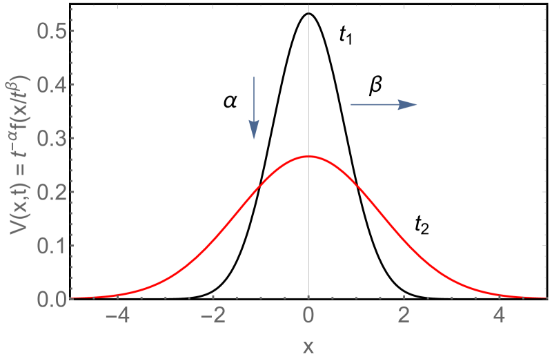
Figure 1: A self-similar solution of Eq. (3.1) for $t_{1}<t_{2}$. The presented curves are Gaussians for regular heat conduction.

The most powerful result of this ansatz is the fundamental- or Gaussian-solution of the Fourier heat conduction equation (or for Fick’s diffusion equation) with $\alpha=\beta=1/2$, which is clearly presented on Figure 1. This transformation is based on the assumption that a self-similar solution exists, i.e., every physical parameter preserves its shape during the expansion. Self-similar solutions usually describe the asymptotic behavior of an unbounded or a far-field problem; the time $t$ and the space coordinate $x$ appear only in the combination of $f(x/t^{\beta})$. It means that the existence of self-similar variables implies the lack of characteristic length and time scales. These solutions are usually not unique and do not take into account the initial stage of the physical expansion process. These kind of solutions describe the intermediate asymptotic of a problem: they hold when the precise initial conditions are no longer important, but before the system has reached its final steady state. For some systems it can be shown that the self-similar solution fulfills the source type (Dirac-delta) initial condition, but not in our next case. They are much simpler than the full solutions and so easier to understand and study in different regions of parameter space. A final reason for studying them is that they are solutions of a system of ordinary differential equations and hence do not suffer from the extra inherent numerical problems of the full PDEs. In some cases self-similar solutions helps to understand diffusion-like properties or the existence of compact supports of the solution.

In the last decade we successfully applied this ansatz for numerous physical systems like heat conduction [36], non-linear Maxwell equation [37] especially multidimensional Euler and Navier – Stokes equations [14, 15] or the Madelung – Schrödinger quantum fluid equations [16] ending up with Refs. [38, 39].

For our system we apply the following notations for the two shape functions in natural units

$$u=t^{-\alpha}f\left(\frac{r}{t^{\beta}}\right)\ \ \ \ \textrm{and}\ \ \ \ \rho=t^{-\gamma}g\left(\frac{r}{t^{\beta}}\right),\>\>$$ (3.2)

where the new variable is $\omega=r/t^{\beta}$.

Calculating time and spatial derivatives of the eqs. (3.2) and substituting to eqs. (2.1) and using the relation, $r=\frac{r}{t^{\beta}}t^{\beta}=\omega t^{\beta}$, and finally we get the next non-linear ordinary differential equation (ODE) system

$$g-\omega g^{\prime}+f^{\prime}g+fg^{\prime}+\frac{2gf}{\omega}=0,$$

$$-\omega f^{\prime}+ff^{\prime}=-w\frac{g^{\prime}}{g}-\frac{g^{\prime}}{\omega}+\frac{g}{\omega^{2}},$$ (3.3)

where prime means derivation with respect to $\omega$.

For the initially free three self-similar exponents $\alpha$, $\beta$, and $\gamma$ we obtained the following numerical values: $\alpha=0$, $\beta=1$, and $\gamma=-1$. This means that dynamical variables, velocity and density, have spreading property as time goes on ($\beta=1$). Our physical intuition says that spreadings are somehow similar to expansion which is a basic property of the Universe. The two ”decay” exponents ($\alpha$ and $\gamma$) are however not positive, which means that the magnitude of the velocity, $u$ remains the same even for large times. Density, $\rho$ is even more peculiar, the magnitude linearly enhances in time. We note the usual decaying and dispersive solutions with zero asymptotic values.

The analysis of the relations among the self-similar exponents can end up with three different scenarios:

• The linear algebraic equation system among the exponents are overdetermined, which automatically means contradiction. Therefore the system has inherently no physically self-similar power-law decaying or exploding solutions. Such systems are rare but some damped wave equations e.g. telegraph equations are so.

• All exponents have well-defined numerical values, the analysis of the solutions is straightforward, the remaining coupled non-linear ODE system can be analyzed, in some lucky cases even it can be decoupled and in best cases all variables can be expressed with analytic formulas.

• The linear algebraic equation system for the exponents are under-determined, leaving usually one self-similar exponent completely free, which means an extra free parameter in the obtained ODE system, causing a very rich mathematical structure. The free exponent can have either positive or negative sign. Negative values usually result in power-law divergent or exploding solutions in contrary, positive exponents mean power-law decaying solutions which are desirable for dissipative systems.

In our former works we mostly analyzed viscous fluids like incompressible or compressible viscous Newtonian fluids where all exponents had positive values, which is also true for the regular diffusion process, where $\alpha$ and $\beta=1/2$. In our recent case these values are rather expected to be negative since the observed, approximately-flat Eucledian Universe scenario.

Our present ODE system of equations (3.3) cannot be separated and solved with analytic means. Non-autonomous ODE systems can be linearized and the stationer points can be found which helps to sketch the global qualitative properties of the solutions in the phase space. No such mathematical method exists for non-autonomous non-linear systems. Therefore there is no general tool in our hands that could help us to determine the global properties of the fluid. The equations of the stationary points however can be given as $f^{\prime}(\omega)=0$ and $g^{\prime}(\omega)=0$, then we obtain

$$g\omega+2fg=0,$$

$$g^{2}=0.$$ (3.4)

From the first equation for $g\neq 0$ case we get that the $f=-\frac{\omega}{2}$ function contains the stationary points, with the dimensional definition of velocity, $r/2t$, with lack of information on the general properties of the solutions. From the second equation one can get that $g=0$ is stationary point, which is a trivial statement meaning that zero density is a stationery point.

We do not even know if this ODE system has mathematically rigorous existence and unicity theorem for the solutions. The only physically reasonable way that we can follow is to performed numerous calculations with large number of parameter sets to explore the properties of the solutions in wide range. Our numerical experiences say that both field variable has continuous solution on a closed interval on the half axis of time and radial distance. We found no compact supports or ruptures in the solutions.

4 Results

To understand the physics of the presented model a systematic parameter study of eq. (3.3) is required. First we investigate the role of the $w$ which is the strength of the linear equation of state as well.

Figure 2 presents the density and velocity shape functions for four physically relevant different EoS strength parameters, $w=-1$, $-0.33$, $0$, and $0.33$. We integrate the ODE system between $\omega_{min}=1\cdot 10^{-3}$ and $\omega_{max}=5\cdot 10^{1}$. As initial conditions for velocity and density we took $f(\omega_{min})=0.5$ and $g(\omega_{min})=0.01$. The ratio $f(\omega_{min})/g(\omega_{min})$ was set to 50 here. This choice of the initial velocity (a positive value) means an initially radially expanding fluid, and a physically reasonable positive density. We found, that all four dashed $f(\omega)$ velocity curves are constant and indistinguishable at this range and line widths. All four solid, $g(\omega)$ density curves have a linear dependence of $\omega$.

From now on we fix $w=-1$ which is the choice of the dark matter.

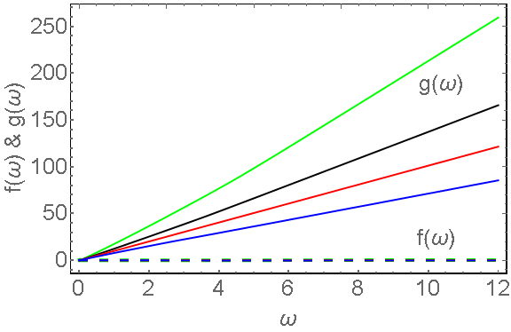
Figure 2: The shape functions of Eq. (3.3) for different EoS strength parameters: $w=-1$ (green), $-0.33$ (black), $0$ (red), and $0.33$ (blue). The solid and dashed lines represent shape functions of density $g(\omega)$ and velocity $f(\omega)$, respectively. Note, all velocity curves coincide. The initial conditions are $f(10^{-3})=0.5$ and $g(10^{-3})=0.01$.

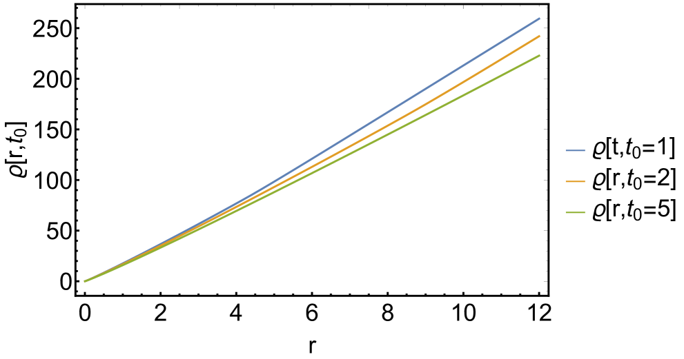
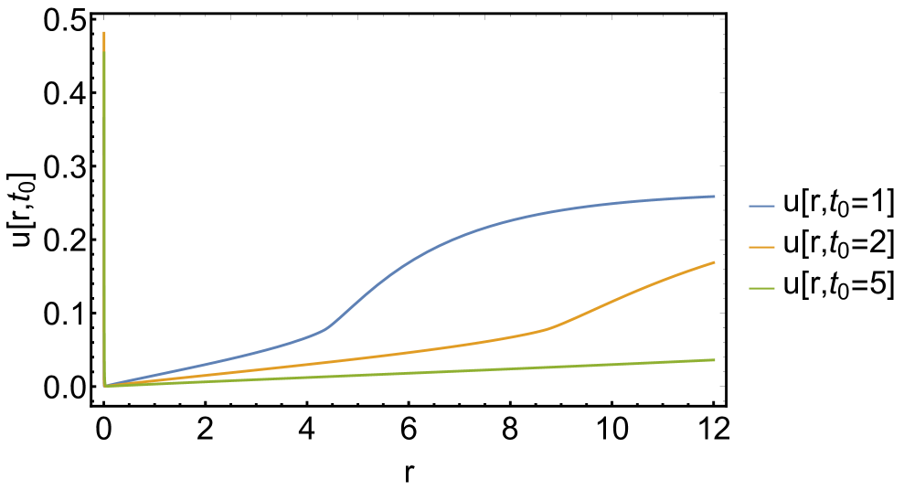
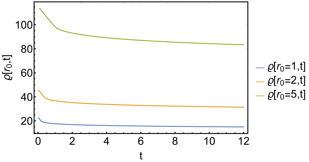
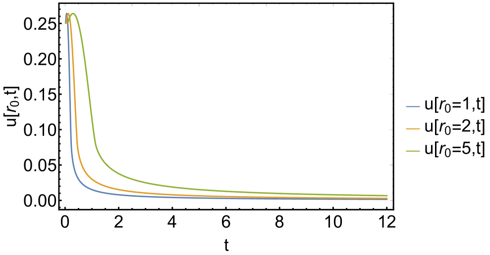
Figure 3: The space-time evolution of the density (left) and the velocity (right) distributions for the case, $w=-1$. Curves are for the radial (top panels) and time (bottom panels) dependence at different fixed time- and space points. The initial conditions are $f(10^{-3})=0.5$ and $g(10^{-3})=0.01$.

Figure 3 shows the space and time projections of the obtained density and the radial velocity distributions in natural units. Upper panels are the radial (space) evolution of the density (left) and radial velocity (right) functions. Lower panels present the time-projections of the above distributions at fixed radius values, respetively.

The density has linear dependence of the radius at any time. The radial dependencde of velocity function looks however a bit more different: at very small distances close to the origin for all time points it has a sharp down running edge with a minima and a linear dependece at larger distances.

The time dependeces are different. The density has a quick but linear decay at small times and another but more slower (and almost linear) decay at larger times. The velocity shape functions start at non-zero values and have a quick deacy in time at all distances. These properties cannot be anticipated directly from the shape functions. We note, these are the direct results of our presented model with initial conditions for the same point, $f(\omega_{min}=10^{-3})=0.5$ and $g(\omega_{min}=10^{-3})=0.01$.

It is more relevant to investigate the dynamics of the complete fluid in time and space to understand some general trends or physical phenomena as the function of the initial conditions. For this reason one can calculate the total energy density of the system including the kinetic and potential terms,

$$E_{tot}=E_{kin}+E_{pot}=\frac{1}{2}u^{2}\rho-\frac{\rho}{r}\ .$$ (4.1)

Figure 4 presents the kinetic, $E_{kin}$ and the potential energy, $E_{pot}$ densities – the two reasonable physical quantities which can be evaluated from the hydrodynamical model for a given parameter set. The kinetic energy is zero in the origin, has a linearly enhancing maxima at larger distances and has a quick decay in time for all radial distances. This means parctically a blowing up sphere where the fluid moves. The potential energy has different properties, finitie values in the origin at practically all times, and a slow decay for large times and distances.

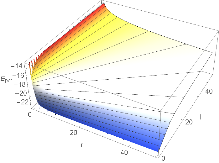
Figure 4: The kinetic and potential energy densities of the investigated fluid for $w=-1$, with initial conditions $f(10^{-3})=0.5$ and $g(10^{-3})=0.01$.

Since the solutions of our non-autonomous non-linear ODE system is not known, we investigated how the solutions are depend on the initial conditions. By our analysis different physical scenarios available if we drastically change the ratio of the initial velocity and density. Another point is the effect of the changing the sign of the initial velocity. Positive sign means expansion, which may be stopped later, while negative sign result in an initial collapse of the fluid.

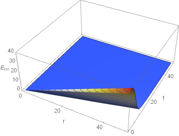
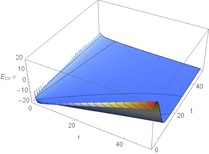
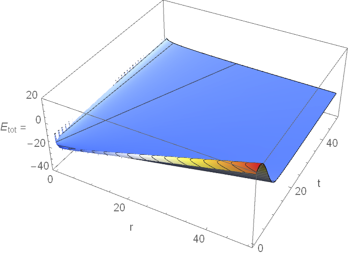
Figure 5: The first column presents the kinetic energies and the second is for the total energies calculated with different initial velocities for the same initial density of $g(10^{-3})=10^{-1}$, and for $w=-1$. The five following rows show the corresponding physical quantities for $f(10^{-3})=-0.5$, $0$, and $0.5$ initial velocities, respectively.

Figure 5 depicts three different kinetic and total energy density distributions of the fluid under each other for different $f(\omega_{min}/g(\omega_{min})$ ratios. The initial density is fixed to 0.01 for all five cases. For a better comparison the both the time and the space domains were taken: $[0,50$] in natural units for all panels. The chosen ranges are varies, because it is not possible to present all functions in the same range in an informative manner.

$f(\omega_{min})=-0.5$

case is seen in the first line panels with setting the kinetic-to-potential energy ratio to -50. Both physical quantity changed radically. The feature that the center of the fluid gains more and more kinetic and potential energy density is much more suppressed, on the other side at small times the kinetic energy density of the total fluid enhances. The larger the radius the larger the energy density gain. Note, that the values of the maximum linearly enhance with time. We may say, that this phenomena is a kind of ”delayed” acceleration and deceleration of the fluid due to the enhanced potential energy density. This effect is not visible for larger initial velocities, where the initial kinetic energy densities dominates the potential energy. In this scenario the strength of the two energy density terms lies in almost in the same range. The figure of the total energy density function is drastically different to the former case, since it become negative everywhere. The effect of the kinetic energy density for small time values at any radius are clearly seen as a ”bump” which lifts the potential energy density. The same statements are valid also for the panel of the third line panels, where the dynamics for small positive initial velocity case, $f(\omega_{min})=+0.5$ is presented.

$f(\omega_{min})=0$

case describes the dynamics of a fluid with zero initial velocity (middle panels). Here the effect of the potential energy density can be studied in a non-perturbed way. The ”bump” of the kinetic energy color density for small times at all fluid radius – a short acceleration and deceleration – of the fluid is originated by the gravitational potential of the fluid itself.

We must summarize our results as follows: for this ideal hydrodynamical model, which does not include any kind of viscous damping, the self-similar ansatz may give solutions which explode in time, if the initial conditions are so.

5 Discussion

The analytical solution was motivated by the cosmological observations. The Hubble-law provides a velocity scaling [40] for the expansion of the Universe, numerous possible scaling mechanisms are coded in our model via the choice of the self-similar ansatz several exponents can describe various time decay scenarios. As Figure 2 presented a linear scale parameter is obtained. Although, the scaling curves are linear everywhere, at around a certain $r$ values a quick change in the velocity is provided naturally as an in-coded inflation-like behavior by the ansatz . This critical $r$ value depends on the initial condition. As right panels of Figure 3 shows high initial velocity in the dark-fluid, $w=-1$ limit (iii), will relax to a small, constant ’non-relativistic’ value at long timescale. Meanwhile, the dependence on the distance is getting saturated and close to flat at far distances from the initial ’Big Bang’ point. We have found, that it is $\lesssim 1\%$ effect for nearby objects. This precision however, well beyond the uncertainty of the measured Hubble-constant value [41, 42, 43, 44] All $u[r_{0},t]$ curves in the lower right part of Figure 3 are getting fully flat beyond $r=2-4$.

The solution for the local density scaling is increasing in space but flat in time. This results the space-time density evolution function in the left panels of Figure 3. Around the center this function starts linearly with the distance, and after a rapid rise, the density of the fluid is getting flat. An interesting feature of the model, that apart from the initial point, the local density is increasing with time – due to the dispersing shock-wave and the dark matter equation of state ($w=1$).

The structure of the ODE and the choice of the initial conditions leave us enough freedom for the valid physical picture. As we could see, the $E_{tot}\approx 0$ is well supported by the solution, especially in the infinite space-time limit presented in Figure 5.

One may also set the initial condition according to that the Universe is observed as flat Euclidean, with $\Omega=\overline{\rho}_{i}/\rho_{c}\approx 1$, and indeed,

$$\Omega=\Omega_{M}+\Omega_{\Lambda}\ \ \textrm{where}\ \ \Omega_{M}=\Omega_{B}+\Omega_{CDM}\ .$$ (5.1)

Here $\Omega_{i}=\overline{\rho}_{i}/\rho_{c}$ for ’$i$’: baryonic ($B$) and cold-dark matter ($CDM$), as well as dark energy ($\Lambda$), respectively. Thus, we can set the asymptotic flat value for the ratio of the kinetic and total energy of the Universe [23, 24, 25],

$$E_{kin}/E_{tot}\sim\Omega_{M}/\Omega\approx 0.27\ .$$ (5.2)

Seemingly, our solution can be compatible with a realistic cosmological picture with fine-tuned initial conditions, which can draw further consequences of the evolution of a early dark-fluid Universe. For $f(\omega_{0}=0.01)=0.1$ and $g(\omega_{0}=0.01)=0.1$ initial condition we get an $E_{kin}/E_{tot}=0.26$ ratio for $r=58$ and $t=2$ spatial coordinate and time point, which can be scaled to the present status of the Universe.

6 Summary and outlook

We presented and analyzed a model where the spherically symmetric compressible Euler equation was used with a general linear matter equation of state and gravitation. This model with $w=-1$ is the simplest candidate for dark fluid. As a method of investigation we applied the self-similar ansatz, which might fullfills the expected ratio of $E_{kin}/E_{tot}\approx 0.27$ depending on the choice of initial conditions.

Further work is in progress to improve our hydrodynamical model, e.g. including fluctuations [45], rotation, relativistic or two-fluid effects [46, 47] or quantum mechanical effects [48] in the near future.

References

- [1] F. Zwicky, Helv. Phys. Acta. 6, 110 (1933).
- [2] J. Einasto, A. Kaasik and E. Saar, Nature 250, 309 (1974).
- [3] J.P. Ostriker, P.J.E. Peebles and A. Yahill, Astrophys. J. (Letters) 193, L1 (1974).
- [4] V.C. Rubin, W.K. Ford Jr. and N. Thonnard, Astrophys. J. Lett. 225, L107 (1978).
- [5] G. Bertone, Particle Dark Matter, Cambridge University Press, 2010.
- [6] R.H. Sanders, The Dark Matter Problem, A Historical Perspective, Cambridge University Press 2010.
- [7] D. Majumdar, DARK MATTER An Introduction CRC Press 2015.
- [8] I.F. Barna, arXiv:gr-qc/0608054.
- [9] C. F. C. Brandt, L. M. Lin, J. F. Villas da Rocha and A. Z. Wang, Int. J. Mod. Phys. D 11, 155-186 (2002)
- [10] C. F. C. Brandt, M. F. A. da Silva, J. F. Villas da Rocha and R. Chan Int. J. Mod. Phy. D 12(7) 1315-1332 (2003)
- [11] M. Heydari-Fard and H. R. Sepangi, JCAP 02, 029 (2009)
- [12] T. Worrakitpoonpon, Mon. Not. Roy. Astron. Soc. 446, 1335-1346 (2015)
- [13] L. Sedov, Similarity and Dimensional Methods in Mechanics CRC Press 1993.
- [14] I.F Barna, Commun. Theor. Phys. 56, 745 (2011).
- [15] I.F. Barna and L. Mátyás, Fluid. Dyn. Res. 52, 015515 (2020).
- [16] I.F. Barna, M.A. Pocsai and L. Mátyás, Journal of Generalized Lie Theory and Applications, 11, 1000271 (2017).
- [17] R. Tabensky and A.H. Taub, Commun. math. Phys. 29, 61 (1973).
- [18] D. Christodoulos, Arch. Rational Mech. Anal. 130, 343 (1995).
- [19] B. Ducomet, E. Feireisl, H. Petzeltov and I. Straskraba, Discrete and Continuous Dynamical Systems, 11, 113 (2004).
- [20] S. Ahmad, A. Rehman Jami and M. Z. Mughal, Modern Physics Letters A, 33, 1850095 (2018)
- [21] D. Giordano, P. Amodio, F. Iavernaro, A. Labianca, M. Lazzo, F. Mazzia, L. Pisani, European Journal of Mechanics / B Fluids 78, 62 (2019).
- [22] N. Deruelle and J.-P. Uzan Relativity in Modern Physics, Oxford University Press, 2018.
- [23] D. Valev, Physics International, 5(1), 15-20. (2014)
- [24] Peacock J. A. et al., Nature, 410 169-173 (2001)
- [25] Hinshaw G. et al., Astrophys. J. Suppl. Series, 180, 225-245 (2009)
- [26] K. Freese et al., Reports on Progress in Physics, 79, 6 (2016)
- [27] G. Rácz, I. Szapudi, I. Csabai and L. Dobos, [arXiv:2006.10399 [astro-ph.CO]].
- [28] R. Emden, Gaskugeln: Anwendungen der mechanischen Wärmetheorien, B.G. Teubner 1907.
- [29] G.P. Horedt, Polytropes Applications in Astrophysics and Related Fields, Kluver Academic Publishers, 2004. Phys. Rev. D 69, 123524 (2004).
- [30] D. Perkovic and H. Stefancic, Phys. Lett. B 797, 134816 (2019).
- [31] J. Hogan, Nature 448, 240 (2007).
- [32] A. Vikman, Phys. Rev. D. 71, 023515 (2005).
- [33] J. Frieman, M. Turner and D. Huterer, Ann. Rev. Astron. Astrophys. 46, 385 (2008).
- [34] G.I. Baraneblatt, Similarity, Self-Similarity, and Intermediate Asymptotics Consultants Bureau, New York 1979.
- [35] Ya. B. Zel’dovich and Yu. P. Raizer Physics of Shock Waves and High Temperature Hydrodynamic Phenomena Academic Press, New York 1966.
- [36] I.F. Barna and R. Kersner, J. Phys. A: Math. Theor. 43, 375210 (2010).
- [37] I.F. Barna, Laser Phys. 24, 086002 (2014).
- [38] D. Campos (editor) Handbook of Navier-Stokes Equation Theory and Applied Analyis Nova Publishers, Chapter 16, Page 275 - 304 (2017).
- [39] Valentino Simpao and Hunter C. Little (editors) Understanding the Schrödinger Equation Some Non[Linear] Perspectives, Nova Publishers, Chapter 6, Page 181 - 224 (2020).
- [40] Hubble, E. Proceedings of the National Academy of Sciences. 15 (3): 168–73. (1929)
- [41] Freedman, W. L.; et al. Astrophysical Journal. 553 (1): 47–72. (2001)
- [42] Jarosik, N.; et al. Astrophysical Journal Supplement Series. 192 (2): 14 (2011)
- [43] Bucher, P. A. R.; et al. (Planck Collaboration) (2013). ”Planck 2013 results. I. Overview of products and scientific Results”. Astronomy & Astrophysics. 571:
- [44] The LIGO Scientific Collaboration and The Virgo Collaboration; Nature. 551 (7678): 85–88 (2019)
- [45] A. Kovács, R. Beck, I. Szapudi, I. Csabai, G. Rácz and L. Dobos, MNRAS 499(1), 320–333 (2020)
- [46] T. Harko and F. S. N. Lobo, Phys. Rev. D 83, 124051, (2011).
- [47] I.F. Barna and L. Mátyás, accepted in Mathematical Modelling and Analysis 2021 march, arXiv:2004.09815.
- [48] E. Madelung, Zeitschrift fur Physik, 40, 322 (1927).