Supplemental Studies for Simultaneous Goodness-of-Fit Testing

Abstract

Testing to see whether a given data set comes from some specified distribution is among the oldest types of problems in Statistics. Many such tests have been developed and their performance studied. The general result has been that while a certain test might perform well, aka have good power, in one situation it will fail badly in others. This is not a surprise given the great many ways in which a distribution can differ from the one specified in the null hypothesis. It is therefore very difficult to decide a priori which test to use. The obvious solution is not to rely on any one test but to run several of them. This however leads to the problem of simultaneous inference, that is, if several tests are done even if the null hypothesis were true, one of them is likely to reject it anyway just by random chance. In this paper we present a method that yields a p value that is uniform under the null hypothesis no matter how many tests are run. This is achieved by adjusting the p value via simulation. We present a number of simulation studies that show the uniformity of the p value and others that show that this test is superior to any one test if the power is averaged over a large number of cases.

Keywords: Kolmogorov-Smirnov, Anderson-Darling, Shapiro-Wilk, Neyman Smooth test, Power, Monte Carlo Simulation

1 Introduction

A goodness-of-fit test is concerned with the question whether a data set has been generated by a certain distribution. It has a null hypothesis of the form $H_{0}:F=F_{0}$, where $F_{0}$ is a cumulative distribution function. For example, one might wish to test whether a data set comes from a standard normal distribution. An obvious and usually more useful extension is to test $H_{0}:F\in\mathscr{F}_{0}$ where $\mathscr{F}_{0}$ is a family of distributions but without specifying the parameters. So one might wish to test whether a data set comes from a normal distribution but without specifying the mean and standard deviation.

As described above a goodness-of-fit test is a hypothesis test in the Fisherian sense of testing whether the data is in agreement with a model. The main issue with this approach is that it does not allow one to decide which of two tests is better, that is has the higher power. To solve this problem Neyman and Pearson in the 1930s introduced the concept of an alternative hypothesis, and most tests done today follow more closely the Neyman-Pearson description, although they often are a hybrid of both. The original Fisherian test survives mostly in the goodness-of-fit problem, because here the obvious alternative is $H_{a}:F\not\in\mathscr{F}_{0}$, a space so huge as to be useless for power calculations.

The goodness-of-fit (gof) test is one of the oldest and most studied problems in Statistics. For an introduction to Statistics and hypothesis testing in general see [11] or [6]. For discussions of the many goodness-of-fit tests available see [12], [30], [36] and [33]. [33] has an extensive list of references on the subject.

2 The Tests

Many goodness-of-fit methods have been developed over time. In this section we will briefly discuss those currently implemented in our method. Let $n$ be the sample size and $x_{1},..,x_{n}$ the ordered data set. Let $F$ be the distribution function specified under the null hypothesis, either with all parameters fixed or with parameters estimated from the data.

1. Chi-square tests: this is the oldest gof test, dating back to Pearson [28]. It was originally invented for discrete data and applying it to continuous data requires that the data be binned. This can be done in an infinite number of ways, and many studies have investigated the effect of the binning on both the null distribution and on the power of this test, see for example [35], [5], [9], [13], [17], [18], [21], [22], [27], [25], [29] and [34].

   The two most commonly used methods are bins of equal size (except for a few bins with exceptionally low numbers of observations) and bins with equal counts or probability under the null. Also numerous formulas for the number of bins have been developed. [31] discuss a novel binning scheme and show that relatively few bins are often best. We will use their binning scheme with $k=5+m$ bins and $\kappa=0.5$, where m is the number of parameters estimated from the data. The routine can also use equal size and/or equal probability bins with a number of bins chosen by the user.

   A large number of tests are based on a measure of the distance between the distribution function specified under the null hypothesis and the empirical distribution function:

2. Kolmogorov-Smirnov KS: next to the chi-square test this is clearly the most commonly employed gof test. The test statistic is give by

   $$KS=\max\{i/n-F(x_{i}),F(x_{i})-(i-1)/n\}$$

   For further discussions see [7], [16] and [24].

3. Anderson-Darling AD

   $$AD=-n-\frac{1}{n}\sum_{i=1}^{n}(2i-1)\left(\log(F(x_{i})+\log(1-F(x_{n+1-i})\right)$$

   For further details see [3] and [4]

4. Cramer-vonMises CM

   $$CM=\frac{1}{12n}+\sum_{i=1}^{n}\left(\frac{2i-1}{2n}-F(x_{i})\right)^{2}$$

   For further details see [2]

5. Wilson W

   $$CM=\frac{1}{12n}+\sum_{i=1}^{n}\left(\frac{2i-1}{2n}-F(x_{i})\right)^{2}-n(\bar{F(x}-\frac{1}{2})^{2}$$

   [36] studies three test statistics based on likelihood ratios:

6. Zhang ZK

   $$ZK=\max\{(i-0.5)\log\frac{i-0.5}{nF(x_{i})}+(n-i+0.5)\log\frac{n-i+0.5}{n(1-F(x_{i}))}\}$$

7. Zhang ZA

   $$ZA=(-1)\sum_{i=1}^{n}\frac{\log F(x_{i})}{n-i+0.5}+\frac{\log 1-F(x_{i})}{i-0.5}$$

8. Zhang ZC

   $$ZC=\sum_{i=1}^{n}\left(\frac{\log(1/F(x_{i})-1)}{(n-0.5)(i-0.75)-1}\right)^{2}$$

   Next we have a method based on the correlation between the ordered data and and the quantiles of the distribution:

   Let $p_{i},i=1,..,n$ be the points calculated by the R routine ppoints, see [8], and let $q_{i}=F^{-1}(p_{i})$, then

9. Probability Plot Correlation Coefficient ppcc

   $$pp=1-cor(x,q)$$

   This test was discussed in [14]. Note we changed to 1-cor(x,q) from the usual definition cor(x,q) so that large values of the test statistic will lead to rejection of the null hypothesis. The same is also true for the next test:

10. Shapiro-Wilk SW

    This test was specifically developed for the normal distribution, see [32]. We use the R routine shapiro.test to find the value of the test statistic.

    Also designed specifically for the normal distribution is the

11. Jarque-Bera test JB

    $$\hat{\mu}_{k}=\frac{1}{n}\sum_{i=1}^{n}(x_{i}-\bar{x})^{k}$$

    $$S=\frac{\hat{\mu}_{3}}{\hat{\mu}_{2}^{3/2}}$$

    $$K=\frac{\hat{\mu}_{4}}{\hat{\mu}_{2}^{2}}$$

    $$JB=\frac{n}{6}(S^{2}+(K-3)^{2}/4)$$

    see [20]

12. Neyman Smooth tests

    Finally we use the Neyman smooth tests implemented in the R package ddst for the cases of the normal, uniform and exponential distributions, see [26], [23] and [19].

Some of these tests such as KS and AD are distribution-free when the null hypothesis specifies the distribution completely. That is, in those cases the test statistics have distributions that are known analytically. In our routine, however, we will not make use of this feature. This is because for others the null distribution always has to be found via simulation, and simply doing so for all tests adds a negligible computational effort. Moreover, even those tests loose their distribution-free property in the more interesting case where only the form of the distribution is specified but parameters have to be estimated in some way.

It is very simple to add other tests to our routine. All that is needed is to add some R code to the TS function that calculates the test statistic. However, it is assumed that it is a large value of the test statistic that leads to rejection of the null hypothesis.

3 p value adjustment

Let’s say we carry out $k$ hypothesis tests $H^{1},..,H^{k}$ and let’s assume that all $k$ null hypotheses are in fact true. Let’s denote by $P_{i}$ the p value of the $i^{th}$ test. Before carrying out the test $P_{i}$ is a random variable, and if the underlying distribution is continuous $P_{i}\sim U[0,1]$. We are interested in whether any of the tests rejects the null hypotheses, and we denote by $P$ the p value of this test. Its distribution is given by

$$F_{P}(p)=Prob(P<p)=1-Prob(P>p)=1-Prob(P_{i}>p;i=1,..,k)$$

If all these tests were independent we would find

$$F_{P}(p)=1-\prod_{i=1}^{k}Prob(P_{i}>p)=1-(1-p)^{k}$$

Finally using the probability integral transform we could adjust the p value so that the new p value $F(P)=1-(1-P)^{k}$ would again have a uniform [0,1] distribution. This is of course the basis for the Bonferroni correction, where one often also uses the Taylor approximation $1-(1-x)^{k}\approx kx$ and then adjusts the type I error probability of the individual tests to $\alpha/k$.

Clearly though in our case the tests are not independent because it is the same data set in all of them. Therefore we do not know what $F_{P}$ is. We can however estimate it via simulation: generate a data set according to the distribution under the null hypothesis, possibly using the parameter estimates from the data. Apply each test to the simulated data and find the respective values of the test statistic. Repeat many (say $B=25000$) times. Next generate another data set and find the p values as the percentage of test statistics that are larger than this one for each test. Find the smallest of the p values. Again repeat this $B$ times. Use the empirical distribution function of these simulated p values $\hat{F}_{P}$ as an estimate of $F_{P}$. In our routine we also use linear interpolation between the jump points of the empirical distribution function. Now find the p value for the actual data, say $p_{D}$, and adjust it by calculating $\hat{F}_{P}(p_{D})$.

This method for adjusting a p value is in fact quite general. As an example, consider the classic problem of pairwise comparisons of group means. As an illustration we generate $100$ observations from a standard normal distribution. Each is assigned at random to one of $5$ groups, so the population group means are in fact all equal to $0$. We then carry out each of the $10$ pairwise comparisons using the two-sample t test and record the smallest p value. The left upper panel of Figure 1 shows the histogram of p values, which are clearly far from uniform. Next we find the empirical distribution function, shown in the upper right panel. Here we also add the curves for $y=x$ and $y=1-(1-x)^{10}$, respectively. These correspond to the distribution functions of a uniform [0,1] (no adjustment needed) and the case of independent tests (Bonferroni adjustment). Clearly the pairwise comparison case is somewhat intermediate. Finally the (interpolated) empirical distribution function is applied to the p values, and the lower left panel shows the histogram of transformed p values, now clearly uniform.

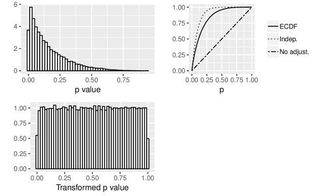
Figure 1: Illustration of p-value transformation for multiple comparisons in ANOVA.

This method for adjusting the p value is of course not new, however it has only recently with the availability of fast computers become doable in many problems. For a general discussion of this idea see [10]. For an application to simultaneous confidence bands in quantile-quantile plots see [1] and an application to goodness-of-fit testing is discussed in [15].

4 Other circumstances

Our routine also allows for two situations sometimes encountered in practice:

4.1 Already binned data

In some fields it is common that the data, although coming from a continuous distribution, is already binned. This is typically the case, for example, in high energy physics experiments because of finite detector resolution. Our routine attempts to ‘recreate‘ the original data by spreading it out within the bins. This is done according to the quantile function if one is provided or uniformly if not.

4.2 Random sample size

Another feature often encountered is that the sample size itself is random. This is the case, for example, if the determining factor was the time over which an experiment was run. Our routine allows this if the sample size is a variate from a Poisson distribution with known rate $\lambda$, as is often the case.

5 Performance

We have carried out a large number of simulation studies to investigate the performance of this method.

5.1 Type I error

Because we use simulation to find the distributions of the test statistics under the null hypothesis as well as the distribution of the minimum p value and the p value adjustment, the method will achieve the nominal type I error probability essentially by construction. Nevertheless, table 1 shows the actual type I error probabilities at the nominal 1%, 5% and 10% levels for a number of null hypotheses. Here each simulation is based on $25000$ runs.

Table 1: Actual type I error probabilities for a number of null distributions, sample sizes and nominal type I error probabilities.

Distribution	Parameters	Sample Size	$1\%$	$5\%$	$10\%$
Normal	Fixed	100	1.1	5.4	10.1
Normal	Fixed	500	1.0	5.4	10.2
Normal	Fixed	1000	1.0	5.0	9.8
Normal	Estimated	100	0.9	4.9	10.0
Normal	Estimated	500	1.2	5.2	10.1
Normal	Estimated	1000	1.2	5.5	10.3
Uniform	Fixed	100	1.1	4.9	10.0
Uniform	Fixed	500	1.1	4.7	9.7
Uniform	Fixed	1000	0.9	4.8	10.0
Exponential	Fixed	100	1.2	5.2	10.0
Exponential	Fixed	500	1.0	4.9	10.1
Exponential	Fixed	1000	1.1	5.2	10.3
Exponential	Estimated	100	1.0	5.0	10.0
Exponential	Estimated	500	1.0	4.4	9.4
Exponential	Estimated	1000	1.1	5.3	10.5
Beta	Fixed	100	1.1	5.1	10.5
Beta	Fixed	500	1.1	5.1	9.8
Beta	Fixed	1000	1.1	4.9	9.7
Gamma	Fixed	100	1.0	5.1	10.2
Gamma	Fixed	500	1.0	4.9	9.6
Gamma	Fixed	1000	1.1	4.9	9.9

5.2 Power

Next we discuss a number of case studies for the power of this method. In all of them the sample size is $1000$, the null distribution is found based on $25000$ simulation runs and the power based on $10000$ runs.

The first five cases all specify a normal distribution under the null hypothesis:

5.2.1 Normal vs t

Here the mean and standard deviation are estimated via maximum likelihood. The true distribution is a t distribution with $n=3,6,..,60$ degrees of freedom. The power curves are shown in Figure 2. The method with the highest mean power is JB, followed by ppcc, RC, SW, ZC, ZK, sNor, ZA, AD, W, CdM, KS and RGd. The new RC method is in third place. In all the power graphs it is highlighted by connecting its dots and the legend shows the methods in the order of their mean power.

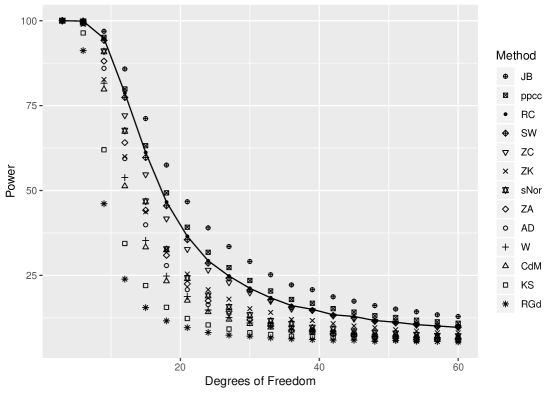
Figure 2: Power of various tests if null hypothesis specifies a normal distribution with parameters estimated and the true distribution is a t with degrees of freedom going from 3 to 60.

5.2.2 Normal(0, 1) vs t, Figure 3

The setup is the same as above but the now the mean and standard deviation are fixed.

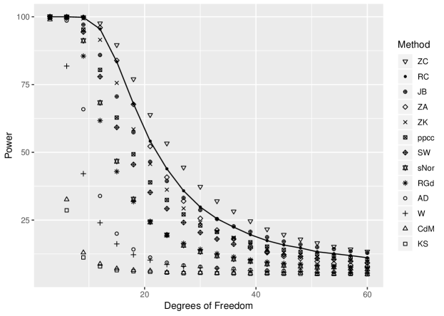
Figure 3: Power of various tests if null hypothesis specifies the standard normal distribution and the true distribution is a t with degrees of freedom going from 3 to 60.

5.2.3 Normal vs Beta(q, q), Figure 4

Mean and standard deviation are estimated via maximum likelihood. The true distribution is a Beta(q, q) distribution with $q=5:24$.

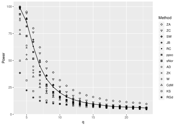
Figure 4: Power of various tests if null hypothesis specifies a normal distribution with parameters estimated and the true distribution is a Beta(q,q).

5.2.4 Normal(r, r) vs Gamma(r, 1), Figure 5

The mean and variance of the normal distribution under the null are fixed at r and r. The data comes from a Gamma(r ,1) distribution, where $r=2*1:20+3$. The power graph is in Figure 5.

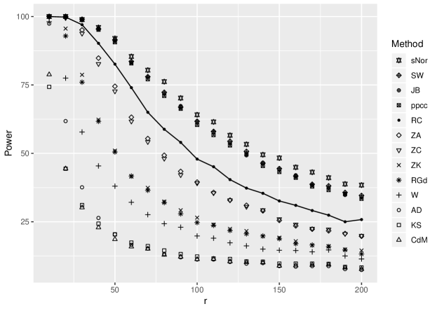
Figure 5: Power of various tests if null hypothesis specifies normal distribution with mean and standard deviation r and the true distribution is a Gamma(r, 1).

5.2.5 Normal vs Gamma(r, 1), Figure 6

Same setup as in the previous example, but now the mean and the standard deviation are estimated via maximum likelihood.

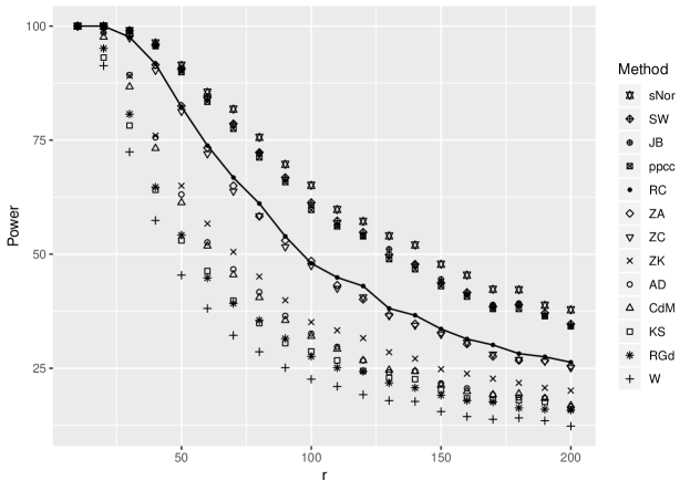
Figure 6: Power of various tests if null hypothesis specifies normal distribution with mean and standard deviation estimated and the true distribution is a Gamma(r, 1).

Next we consider four cases with a uniform distribution under the null hypothesis:

5.2.6 U[0,1] vs Linear(s), Figure 7

The linear density is parametrized as $f(x;s)=2sx+1-s,0<x<1$, so the case $s=0$ corresponds to the U[0,1] distribution.

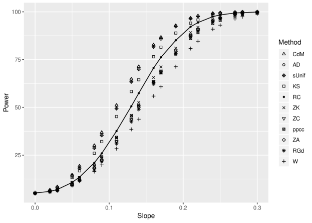
Figure 7: Power of various tests if null hypothesis specifies a Uniform [0,1] and the true distribution is linear.

5.2.7 U[0,1] vs Beta(1,q), Figure 8

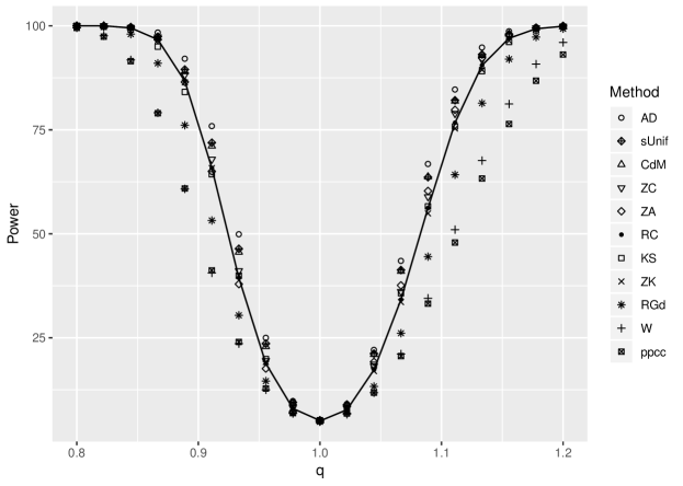
Figure 8: Power of various tests if null hypothesis specifies a Uniform [0,1] and the true distribution is Beta(1,q).

5.2.8 U[0,1] vs Beta(q,q), Figure 9

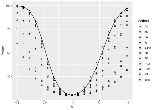
Figure 9: Power of various tests if null hypothesis specifies a Uniform [0,1] and the true distribution is Beta(q,q).

5.2.9 U[0,1] vs Quadratic, Figure 10

The quadratic density is parametrized as $f(x;s)=3a(x-0.5)^{2}+1-a/4,0<x<1$, so the case $a=0$ corresponds to the U[0,1] distribution.

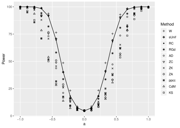
Figure 10: Power of various tests if null hypothesis specifies a Uniform [0,1] and the true distribution is quadratic.

The next four cases use the exponential distribution under the null hypothesis:

5.2.10 Exponential vs Exponential(1)+Normal(1.5, $\sigma^{2}$), Figure 11

Under the true distribution the density has a bump at 1.5. $\sigma=1:20:0.3$. The normal distribution is truncated to $x>0$.

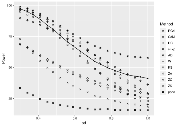
Figure 11: Power of various tests if null hypothesis specifies an exponential distribution with estimated rate and the true distribution is exponential rate 1 with a normal bump mean 1.5 and varying standard deviaiton.

5.2.11 Exponential(1) vs Gamma(p, 1), Figure 12

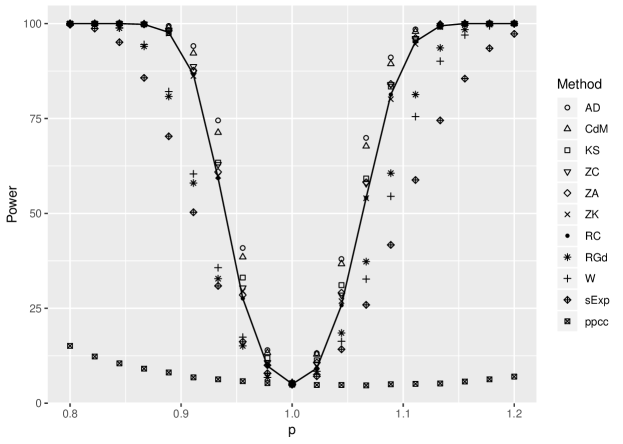
Figure 12: Power of various tests if null hypothesis specifies an exponential distribution with rate 1 and the true distribution is Gamma(p, 1).

5.2.12 Exponential vs Gamma(p, 1), Figure 13

The rate of the exponential is estimated via maximum likelihood.

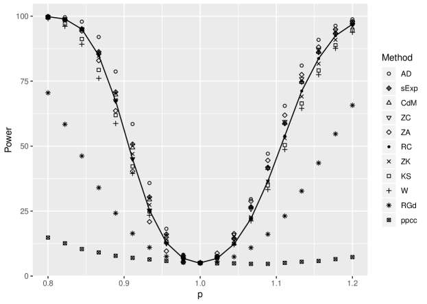
Figure 13: Power of various tests if null hypothesis specifies an exponential distribution with rate estimated and the true distribution is Gamma(p, 1).

5.2.13 Exponential vs Inverse Power, Figure 14

The true density is parametrized as $f(x;a)=\frac{(a+1)}{(1+x)^{a}},x>0$. $a=5:20:30$.

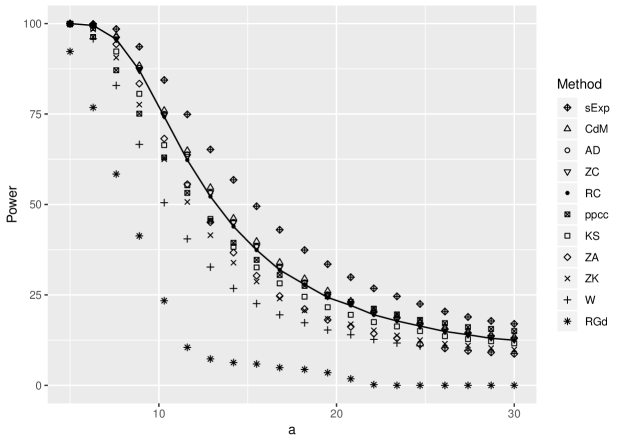
Figure 14: Power of various tests if null hypothesis specifies an exponential distribution with rate estimated and the true distribution is Inverse.

5.2.14 Truncated Exponential(0.5, 0, 1) vs Linear(p), Figure 15

The null hypothesis specifies an exponential distribution rate 0.5, truncated to the interval $[0,1]$. The true distribution is a linear as above, with slope $s=-0.2:20:-0.5$.

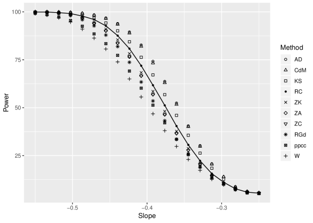
Figure 15: Power of various tests if null hypothesis specifies an exponential distribution with rate 0.5 truncated to [0,1] and the true distribution is linear.

5.2.15 Truncated Exponential(., 0, 1) vs Linear(p), Figure 16

Same as last case, but now the rate is estimated via maximum likelihood.

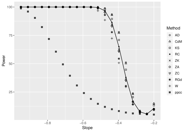
Figure 16: Power of various tests if null hypothesis specifies an exponential distribution with estimated rate, truncated to [0,1], and the true distribution is linear.

5.2.16 Beta(2,2) vs Beta(2,2,p), Figure 17

The true distribution is a non-central Beta with non-centrality parameter $p=0:20:0.75$.

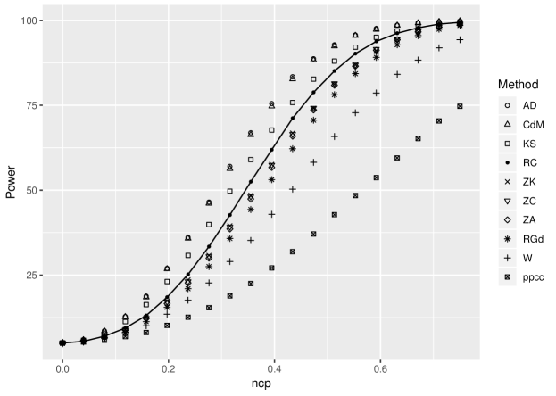
Figure 17: Power of various tests if null hypothesis specifies a Beta( 2,2) and the true distribution is a non central Beta(2,2,p).

5.2.17 Beta(1,.) vs Linear(s), Figure 18

The null distribution is a Beta with $\alpha=1$ and $\beta$ estimated via maximum likelihood.

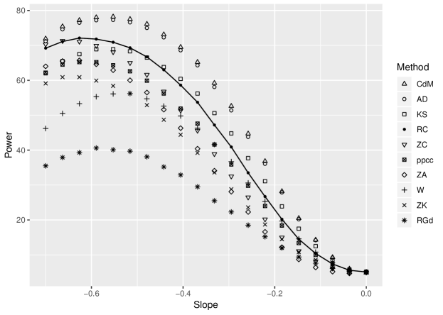
Figure 18: Power of various tests if null hypothesis specifies a Beta (1, $\beta$) with $\beta$ estimated and the true distribution is linear.

5.2.18 Erlang(., .) vs Gamma($\alpha$,5), Figure 19

The null distribution is Erlang with the parameters estimated via method of moments. The true distribution is Gamma($\alpha$,5), where $\alpha=1.75:20:2.25$.

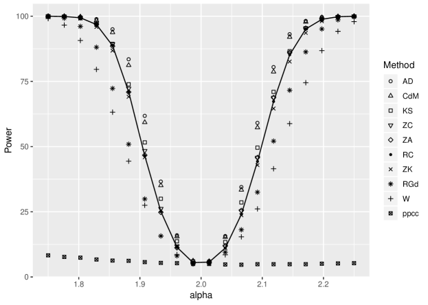
Figure 19: Power of various tests if null hypothesis specifies an Erlang with parameters estimated and the true distribution is Gamma($\alpha$, 5).

5.2.19 Uniform[0,1] vs Beta(1, q), binned data, Figure 20

Here the data is in the form of a histogram with 50 equal-sized bins. $q=0.8:20:1.2$.

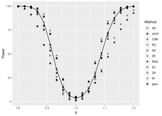
Figure 20: Power of various tests if null hypothesis specifies a Uniform[0,1], the true distribution is Beta(1,q) and the data is binned.

5.2.20 Normal vs t(n), binned data, Figure 21

Again the data is in the form of a histogram with 50 bins. The mean and standard deviation are estimated via maximum likelihood.

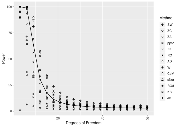
Figure 21: Power of various tests if null hypothesis specifies a normal distribution with ean and standard deviation estimated, the true distribution is t and the data is binned.

5.2.21 Uniform[0,1] vs Beta(1, q), Poisson sample size, Figure 22

In this case the sample size varies according to a Poisson random variable with rate $\lambda=1000$..

Figure 22: Power of various tests if null hypothesis specifies a Uniform [0,1], the true distribution is Beta(1,q) an the sample size is drawn from a Poisson(1000).

5.3 Overall Performance

In this section we compare the performance of the various methods. Note that in almost all cases if method A had higher power than method B for one value of the parameter, it did so for all of them. It is therefore reasonable to compare their mean powers.

5.3.1 Mean Power

Our case studies include 21 different null hypotheses and true distributions, each with 20 different parameter values for a total of 420 cases. If we simply find the mean power of the methods used in all simulations we find that RC has the highest mean power at 49.18%, followed by ZC (48.91%), AD (48.77%), ZA (48.20%), CdM (46.08%), ZK (45.97%), KS (42.66%), W (42.25%), RGd (41.67%) and finally ppcc (35.27%). So the method proposed in this paper achieves the highest average power over the 21 case studies. While any study of this kind is necessarily limited, this does suggest that the RC method performs quite well.

5.3.2 Rankings of Methods by Case

Table 2: Ranking of methods for each case study

	RC	ZC	AD	ZA	CdM	ZK	KS	W	RGd	ppcc
Case 1	9	8	5	6	3	7	2	4	1	10
Case 2	9	10	4	8	2	7	1	3	5	6
Case 3	8	9	6	10	3	5	2	4	1	7
Case 4	9	7	3	8	1	6	2	4	5	10
Case 5	9	7	5	8	4	6	3	1	2	10
Case 6	7	5	9	3	10	6	8	1	2	4
Case 7	6	8	10	7	9	4	5	2	3	1
Case 8	10	9	5	8	3	6	2	7	4	1
Case 9	9	6	7	4	2	5	1	10	8	3
Case 10	8	3	7	4	9	2	5	6	10	1
Case 11	4	7	10	6	9	5	8	2	3	1
Case 12	6	8	10	7	9	5	4	3	2	1
Case 13	7	8	9	4	10	3	5	2	1	6
Case 14	7	4	10	5	9	6	8	1	3	2
Case 15	7	4	10	5	9	6	8	2	3	1
Case 16	7	5	10	4	9	6	8	2	3	1
Case 17	7	6	9	4	10	2	8	3	1	5
Case 18	5	7	10	6	9	4	8	2	3	1
Mean Rank	7.4	6.7	7.7	5.9	6.7	5.1	4.9	3.3	3.3	3.9

Another way to study the performance of the methods is as follows: for each of the 18 null hypotheses (excluding the special cases such as binned data) we rank the methods, with a rank of 1 for the method with the highest mean power. Next we find the number of times a method had rank 1, rank 2 and so on.

The results are shown in table 2, together with the mean rankings over all cases. The RC method has the second highest mean ranking after Anderson-Darling. While Anderson-Darling is certainly a very good method, and would be our choice if only a single method can be used, it also is likely to perform badly in some cases. While we did not find such a case it almost certainly exists. On the other hand by its design RC should never perform especially badly.

Figure 23 also illustrates the rankings, with the methods sorted by their overall mean power. The frequency a rank was attained is indicated by the size of the plotting symbol. RC was ranked best once, second five times, third twice etc. On the other hand RC was never worse than seventh. Four methods (CdM, W, RGd and ppcc) were best in some cases and worst in others, indicating the difficulty to choose a single method.

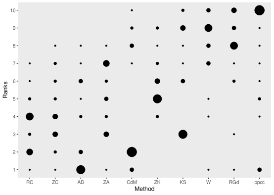
Figure 23: Number of times each method was best, had rank 2 and so on. The size of the plotting symbol indicates the frequency of each rank, 1 being best.

5.3.3 Difference in Power to Best Method

Finally we consider for each case how much lower the power of each method is when compared to the best. To do so we find for each case the value of the parameter where at least one method has a power just over 90%. For this value of the parameter all powers are recorded. They are shown in Figure 24. The power of RC is never less than 80%, or about 10% below the best method whereas the individual methods sometimes perform much worse. Even Anderson-Darling had a power below $50\%$ twice. So using RC guards against ever having exceptionally low power.

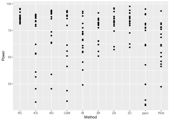
Figure 24: Power of each method when best one has a power just above 90%.

6 Computational Issues

An R library as well as the source code with all necessary routines to carry out this test is available from https://github.com/WolfgangRolke/simgof. Alternatively it can be run as an R shiny app at https://drrolke.shinyapps.io/sgoftest. The app allows the user to upload the data set and define the necessary routines (to calculate the distribution function, generate new data from the distribution for the Monte Carlo, optionally calculate the quantile function and do parameter estimation) either using R or C++ code. The code to run the app locally is also available at https://github.com/WolfgangRolke/simgof and detailed explanations on how to run the app can be found at http://academic.uprm.edu/wrolke/simgof.explained.pdf.

7 Conclusion

We presented a method that combines several standard goodness-of-fit tests for continuous distributions. The test rejects the null hypothesis at the $\alpha$ level if any of the individual tests does. Simulation is used to adjust the p value so it has a uniform [0,1] distribution. Extensive simulation studies show that this method does indeed achieve the desired nominal type I error probability and when averaged over the 21 cases included in this study has overall power better than any of the individual tests. While some methods such as Anderson-Darling and Zhang ZC generally perform well they also can have quite low power whereas RC should never be much worse than the best method, simply because that best method is part of RC.

8 Appendix - Source Code

In the following we have the source code for the routines used.

9 TS

This routine calculates the test statistics for all the tests included.

⬇

TS <- function(x, case) {

if(is.list(x))

x <- simgof::spreadout(x, case)

# data is binned, unbin it

n <- length(x)

x <- sort(x)

param <- case$est.mle(x)

y <- case$pnull(x, param)

m <- 1:n-0.5

out <- rep(0, length(case$methods))

names(out) <- case$methods

tmp <- c( max(c(y-0:(n-1)/n, 1:n/n-y)),

-n-mean((2*1:n-1)*(log(y)+log(1-y[n:1]))),

1/(12*n)+sum( ((2*(1:n)-1)/2/n- y)^2 ),

1/(12*n)+sum( ((2*(1:n)-1)/2/n- y)^2 )-n*(mean(y)-0.5)^2,

max(m*log(m/n/y)+(n-m)*log((n-m)/n/(1-y))),

(-1)*sum(log(y)/(n-m)+log((1-y))/m),

sum(log( (1/y-1)/((n-0.5)/(1:n-0.75)-1) )^2))

names(tmp) <- c("KS", "AD", "CdM", "W", "ZK", "ZA", "ZC")

for(m in case$methods) {

if(m %in% c("KS", "AD", "CdM", "W", "ZK", "ZA", "ZC"))

out[m] <- tmp[m]

}

if("SW" %in% case$methods)

out["SW"] <- 1-shapiro.test(x)$statistic

if("ppcc" %in% case$methods)

out["ppcc"] <- 1-cor(x, case$qnull(ppoints(case$n), param))

if("JB" %in% case$methods) {

mu <- mean(x)

S <- mean((x-mu)^3)/(mean((x-mu)^2))^(3/2)

K <- mean((x-mu)^4)/(mean((x-mu)^2))^2

out["JB"] <- n/6*(S^2+(K-3)^2/4)

}

if("RGd" %in% case$methods) {

out["RGd"] <- chisquare.test(x, case, "RGd")

}

if("Equal␣Size" %in% case$methods) {

out["Equal␣Size"] <- chisquare.test(x, case, "Equal␣Size")

}

if("Equal␣Prob" %in% case$methods) {

out["Equal␣Prob"] <- chisquare.test(x, case, "Equal␣Prob")

}

if("sNor" %in% case$methods) {

out["sNor"] <- ddst::ddst.norm.test(x, compute.p = FALSE)$statistic

}

if("sUnif" %in% case$methods) {

out["sUnif"] <- ddst::ddst.uniform.test(x, compute.p = FALSE)$statistic

}

if("sExp" %in% case$methods) {

out["sExp"] <- ddst::ddst.exp.test(x, compute.p = FALSE)$statistic

}

out

}

10 simgof.test

This routine runs the test

⬇

simgof.test <- function(x, pnull, rnull, qnull=function(x) NULL,

do.estimation=TRUE, estimate = function(x) NULL,

include.methods = c(rep(TRUE, 7), rep(FALSE, 9)),

B=1000, lambda) {

methods <- c("KS", "AD", "CdM", "W", "ZA", "ZK", "ZC",

"RGd", "Equal␣Size", "Equal␣Prob",

"ppcc", "JB", "SW", "sNor", "sUnif", "sExp")

# step 1: do some setup work

param <- NULL

if(do.estimation) param <- estimate(x)

case <- list(B=B,

param = param,

methods = methods[include.methods],

n = ifelse(is.list(x), sum(x$counts), length(x)),

pnull = ifelse(do.estimation, pnull, function(x, param=1) pnull(x)),

rnull = ifelse(do.estimation, rnull, function(n, param=1) rnull(n)),

qnull = ifelse(do.estimation, qnull, function(x, param=1) qnull(x)),

est.mle = estimate,

dta = x

)

# step 2: find null distributions of each test

znull <- matrix(0, B, length(case$methods))

colnames(znull) <- case$methods

for(i in 1:B) {

case$n <- ifelse(missing(lambda), case$n, rpois(1, case$lambda))

znull[i, ] <- simgof::TS(case$rnull(case$n, case$param), case)

}

# step 3: find p values for each test, find their minimum

tmp <- rep(0, length(case$methods))

names(tmp) <- case$methods

pval <- rep(0, case$B)

for(i in 1:case$B) {

xsim <- znull[sample(1:B, 1), ]

for(k in case$methods)

tmp[k] <- sum(xsim[k]<znull[, k])/case$B

pval[i] <- min(tmp)

}

# step 4: find cdf of p values

x <- seq(0, 1, length=250)

y <- 0*x

for(i in 1:250) y[i] <- sum(pval<=x[i])/length(pval)

xy <- cbind(x, y)

adjust <- function(xy, a) {

approx(x=xy[, 1], y=xy[, 2], xout=a, rule=2)$y

}

# step 5: run test on data

TS.data <- simgof::TS(case$dta, case)

pvals <- rep(0, length(case$methods))

names(pvals) <- case$methods

for(k in case$methods)

pvals[k] <- sum(TS.data[k]<znull[, k])/case$B

pvals <- c(adjust(xy, min(pvals)), pvals)

names(pvals)[1] <- "RC"

round(pvals, 4)

}

11 chisquare.test

This routine runs the chisquare test, if desired

⬇

chisquare.test <- function (x, case, which="RGd") {

bin.fun <- function (case, k, kappa) {

n <- case$n

L <- min(case$dta)

R <- max(case$dta)

bins0 <- c(L, case$qnull((1:(k - 1))/k), R)

if (k == 2)

bins1 <- c(L, case$qnull(0.5), R)

else {

if (is.finite(L) & is.finite(R))

bins1 <- seq(L, R, length = k + 1)

if (is.finite(L) & !is.finite(R)) {

R <- case$qnull(1 - 5/n)

bins1 <- c(seq(L, R, length = k), Inf)

}

if (!is.finite(L) & is.finite(R)) {

L <- case$qnull(5/n)

bins1 <- c(-Inf, seq(L, R, length = k))

}

if (!is.finite(L) & !is.finite(R)) {

L <- case$qnull(5/n)

R <- case$qnull(1 - 5/n)

bins1 <- c(-Inf, seq(L, R, length = k - 1), Inf)

}

}

bins <- (1 - kappa) * bins0 + kappa * bins1

if (is.nan(bins[1]))

bins[1] <- (-Inf)

if (is.nan(bins[k + 1]))

bins[k + 1] <- Inf

bins <- bin.adjust(case, bins)

bins

}

bin.adjust <- function (case, bins) {

p <- case$param

E <- case$n * diff(case$pnull(bins, p))

if (all(E > 5)) return(bins)

nbins <- length(E)

repeat {

k <- which.min(E)

if (k == 1) {

bins <- bins[-2]

E[1] <- E[1] + E[2]

E <- E[-2]

}

if (k == nbins) {

bins <- bins[-nbins]

E[nbins - 1] <- E[nbins] + E[nbins - 1]

E <- E[-nbins]

}

if (k > 1 & k < nbins) {

if (E[k - 1] < E[k + 1]) {

bins <- bins[-k]

E[k] <- E[k] + E[k - 1]

E <- E[-k]

}

else {

bins <- bins[-(k + 1)]

E[k] <- E[k] + E[k + 1]

E <- E[-(k + 1)]

}

}

nbins <- nbins - 1

if (all(E > 5)) break

}

bins

}

if(which=="Equal␣Prob") {kappa <- 0;k <- ifelse(is.null(case$nbins), 10, case$nbins)}

if(which=="RGd") {kappa <- 0.5;k <- 5+length(case$param)}

if(which=="Equal␣Size") {kappa <- 1; k <- ifelse(is.null(case$nbins), 10, case$nbins)}

case$dta <- x

if(!is.null(case$param)) case$param <- case$est.mle(x)

bins <- bin.fun(case, k = k, kappa = kappa)

tmpbins <- c(-Inf, bins[2:(length(bins)-1)], Inf)

O <- hist(x, breaks = tmpbins, plot = FALSE)$counts

E <- length(x)*diff(case$pnull(tmpbins, case$param))

sum( (O-E)^2/E )

}

References

- Aldor-Noima et al. [2013] Aldor-Noima, S., L. D. Brown, A. Buja, R. A. Stine, and W. Rolke (2013). The power to see: A new graphical test of normality. The American Statistician 67.
- Anderson [1962] Anderson, T. W. (1962). On the distribution of the two-sample cramer-von mises criterion. Annals of Mathematical Statistics 33(3), 1148–1159.
- Anderson and Darling [1952] Anderson, T. W. and D. A. Darling (1952). Asymptotic theory of certain goodness-of-fit criteria based on stochastic processes. Annals of Mathematical Statistics 23, 193–212.
- Anderson and Darling [1954] Anderson, T. W. and D. A. Darling (1954). A test of goodness-of-fit. JASA 49, 765–769.
- Berkson [1980] Berkson, J. (1980). Minimum chi-square, not maximum likelihood. Ann. Math. Stat 8(3), 457–487.
- Bickel and Doksum [2015] Bickel, P. J. and K. A. Doksum (2015). Mathematical Statistics Vol 1 and 2. CRC Press.
- Birnbaum [1952] Birnbaum, Z. W. (1952). Numerical tabulation of the distribution of kolmogorov’s statistic for finite sample size. JASA 47, 425–441.
- Blom [1958] Blom, G. (1958). Statistical estimates and transformed beta-variables. Wiley/New York.
- Bogdan [1995] Bogdan, M. (1995). Data driven version of pearson’s chi-square test for uniformity. Journal of Statistical Computation and Simulation 52, 217–237.
- Buja and Rolke [2006] Buja, A. and W. Rolke (2006). Calibration for simultaneity: (re)sampling methods for simultaneous inference with applications to functional estimation and functional data. Unpublished Manuscript.
- Casella and Berger [2002] Casella, G. and R. Berger (2002). Statistical Inference. Duxbury Advanced Series in Statistics and Decision Sciences. Thomson Learning.
- D’Agostini and Stephens [1986] D’Agostini, R. B. and M. A. Stephens (1986). Goodness-of-Fit Techniques. Statistics: Textbooks and Monographs. Marcel Dekker.
- Dahiya and Gurland [1973] Dahiya, R. C. and J. Gurland (1973). How many classes in the pearson chi-square test? Journal of the American Statistical Association 68, 707–712.
- Filliben [1975] Filliben, J. J. (1975). The probability plot correlation coefficient test for normality. Technometrics 17, 111–117.
- Gontscharuk and Finner [2016] Gontscharuk, V. and H. Finner (2016). Asymptotics of goodness-of-fit tests based on minimum p-value. Communications is Statistics - Theory and Methods 46(5), 2332–2342.
- Goodman [1954] Goodman, L. A. (1954). Kolmogorov-smirnov tests for psychological research. Psychological Bull 51, 160–168.
- Greenwood and Nikulin [1996] Greenwood, P. E. and M. S. Nikulin (1996). A Guide to Chi-Square Testing. Wiley.
- Harrison [1985] Harrison, R. H. (1985). Choosing the optimum volume of classes in the chi-square test for arbitrary power levels. Indian J. Stat. 47(3), 319–324.
- Inglot and Ledwina [2006] Inglot, T. and T. Ledwina (2006). Towards data driven selection of a penalty function for data driven neyman tests. Linear Algebra and its Appl. 417, 579–590.
- Jarque and Bera [1980] Jarque, C. and A. Bera (1980). Efficient tests for normality, homoscedasticity and serial independence of regression residuals. Economics Letters 6(3), 255–259.
- Kallenberg et al. [1985] Kallenberg, W., J. Ooosterhoff, and B. Schriever (1985). The volume of classes in chi-squared goodness-of-fit tests. Journal of the American Statistical Association 80, 959–968.
- Koehler and Gann [1990] Koehler, K. and F. Gann (1990). Chi-squared goodness-of-fit tests: Cell selection and power. Communications in Statistics-Simulation 19, 1265–1278.
- Ledwina [1994] Ledwina, T. (1994). Data driven version of neyman’s smooth test of fit. J. Amer. Statist. Assoc. 89, 1000–1005.
- Massey [1951] Massey, F. J. (1951). The kolmogorov-smirnov test for goodness-of-fit. JASA 46, 68–78.
- Mineo [1979] Mineo, A. (1979). A new grouping method for the right evaluation of the chi-square test of goodness-of-fit. Scand. J. Stat 6(4), 145–153.
- Neyman [1937] Neyman, J. (1937). Smooth test for goodness of fit. Skand. Aktuarietidskr 20, 149–199.
- Ooosterhoff [2002] Ooosterhoff, J. (2002). The choice of cells in chi-square tests. Statistica Neerlandia 39, 115–128.
- Pearson [1900] Pearson, K. (1900). On the criterion that a given system of deviations from the probable in the case of a correlated system of variables is such that it can be reasonably supposed to have arisen from random sampling. Philosophical Magazine (Series 5) 50, 302.
- Quine and Robinson [1985] Quine, M. and J. Robinson (1985). Efficiencies of chi-square and likelihood ratio goodness-of-fit tests. Annals of Statistics 13, 727–742.
- Raynor et al. [2012] Raynor, J. C., O. Thas, and D. J. Best (2012). Smooth Tests of Goodness of Fit. Wiley Sons.
- Rolke and Gutierrez-Gongora [2020] Rolke, W. and C. Gutierrez-Gongora (2020). A chi-square goodness-of-fit test for continuous distributions against a known alternative. Computational Statistics.
- Shapiro and Wilk [1965] Shapiro, S. S. and M. B. Wilk (1965). An analysis of variance test for normality (complete samples). Biometrika 52(3-4), 591–611.
- Thas [2010] Thas, O. (2010). Continuous Distributions. Springer Series in Statistics. Springer.
- Voinov and Nikulin [2013] Voinov, N. B. and M. Nikulin (2013). Chi-Square Goodness of Fit Test With Applications. Academic Press.
- Watson [1958] Watson, G. S. (1958). On chi-square goodness-of-fit tests for continuous distributions. Journal of the RSS (Series B) 20, 44–72.
- Zhang [2002] Zhang, J. (2002). Powerful goodness-of-fit tests based on likelihood ratio. Journal of the RSS (Series B) 64, 281–294.