Achievable Rates of Opportunistic Cognitive Radio Systems Using Reconfigurable Antennas with Imperfect Sensing and Channel Estimation

Hassan Yazdani, Azadeh Vosoughi,  Xun Gong, 
University of Central Florida
E-mail: h.yazdani@knights.ucf.edu, azadeh@ucf.edu, xun.gong@ucf.edu
Abstract

We consider an opportunistic cognitive radio (CR) system in which secondary transmitter (SUtx) is equipped with a reconfigurable antenna (RA). Utilizing the beam steering capability of the RA, we regard a design framework for integrated sector-based spectrum sensing and data communication. In this framework, SUtx senses the spectrum and detects the beam corresponding to active primary user’s (PU) location. SUtx also sends training symbols (prior to data symbols), to enable channel estimation at secondary receiver (SUrx) and selection of the strongest beam between SUtx–SUrx for data transmission. We establish a lower bound on the achievable rates of SUtx–SUrx link, in the presence of spectrum sensing and channel estimation errors, and errors due to incorrect detection of the beam corresponding to PU’s location and incorrect selection of the strongest beam for data transmission. We formulate a novel constrained optimization problem, aiming at maximizing the derived achievable rate lower bound subject to average transmit and interference power constraints. We optimize the durations of spatial spectrum sensing and channel training as well as data symbol transmission power. Our numerical results demonstrate that between optimizing spectrum sensing and channel training durations, the latter is more important for providing higher achievable rates.

Index Terms:
Achievable rates, beam detection, beam selection, channel estimation, imperfect spectrum sensing, opportunistic cognitive radio system, optimal and sub-optimal transmit power, reconfigurable antennas, training and data symbols.

I Introduction

I-A Literature Review

Cognitive radio (CR) technology improves spectrum utilization and fills the spectral holes, via allowing an unlicensed or secondary user (SU) to access licensed bands in a such way that its imposed interference on license holder primary users (PUs) is restricted [1]. CR systems are mainly classified as underlay CR and opportunistic (or interweave) CR systems. In underlay CR systems, SUs use a licensed frequency band simultaneously with PUs, as long as the interference caused by SUs and imposed on PUs stays below a pre-determined threshold [1, 2, 3]. While underlay CR systems do not require spectrum sensing to detect PUs’ activities, they demand coordination between PUs and SUs to obtain channel state information (CSI), that is not always feasible. In opportunistic CR systems, SUs use a licensed frequency band during a time interval, only if that frequency band is not used by PUs. While opportunistic CR systems do not require coordination between PUs and SUs to acquire CSI corresponding to SU-PU link (and hence the system implementation is easier), they necessitate spectrum sensing to monitor and detect PUs’ activities.

The CR literature mainly assume that SU has access to full CSI of all links for its operation. However, in practice, SU has access only to partial CSI, due to several factors including channel estimation error, mobility of PU or SU, and limitation of feedback channel. Partial (imperfect) CSI has deteriorating effects on the fundamental performance limits of CRs and should not be overlooked. We note that the impact of partial CSI on the performance of underlay and opportunistic CR systems are different, due to inherent distinctions between these two CR systems. For underlay CR systems, several researchers have studied the impact of imperfect CSI on the ergodic capacity [4, 5, 6, 7, 8, 9] and symbol error probability [10]. In particular, references [4, 5, 6] focus on investigating the impact of imperfect CSI of SUtx–PU receiver (PUrx)  link on the optimal transmit power of SUtx that maximizes the constrained capacity of SUtx–SUrx link, where SUtx cannot always satisfy the interference power constraint (due to partial CSI) and has to reduce its transmit power. The authors in [7, 8] considered the impact of partial CSI for both SUtx–PUrx and SUtx–SUrx links on the CR system capacity. Different from [7, 8, 4, 5, 6], [9] discussed the trade-off between channel estimation accuracy and channel estimation duration (time). The authors in [9] studied the optimal transmit power of SUtx and optimal channel estimation duration, such that the capacity of SUtx–SUrx link is maximized, subject to a constraint on interference power imposed on PUrx.

In opportunistic CR systems, spectrum sensing is necessary for detecting PUs’ activities and protecting the PUs against harmful interference. In general, any spectrum sensing (signal in noise detection) technique is prone to errors, that can be described as mis-detection or false alarm probability [11, 12]. On the other hand, imperfect CSI of SUtx–SUrx link due to channel estimation error (even under perfect spectrum sensing) has negative influence on the link capacity. Imperfect spectrum sensing exacerbates the negative effect of imperfect CSI on the link capacity. Hence, for opportunistic CR systems, one needs to study the combined impacts of imperfect spectrum sensing and imperfect CSI on the system performance. Such study presents new challenges, compared with studies that focus on understanding only the effect of imperfect spectrum sensing, when CSI is perfect (or vice versa), on the link capacity. To the best of our knowledge, there are only a few works that have considered the aforementioned combined effects in their system performance analysis [13, 14, 15, 16]. For example in [13] SUtx estimates the received power from PU during sensing-estimation time and monitors PU’s activity. If the spectrum is sensed idle, SUtx with its imperfect CSI of SUtx–SUrx link, sends data to SUrx with a fixed power. The authors showed that the constrained capacity of SUtx–SUrx link can be significantly enhanced (subject to a constraint on the detection probability), via optimizing sensing-estimation time. The authors in [14] considered a delay-sensitive CR system with a different setup, where after spectrum sensing at SUtx, SUtx transmits at fixed powers and rates, where these fixed values depend on the result of spectrum sensing (i.e., the transmit power and rate corresponding to spectrum being sensed idle are different from those corresponding to spectrum being sensed busy). The authors optimized these fixed powers and rates such that the defined effective capacity is maximized, subject to average transmit power and buffer length constraints. The authors in [15] considered a related problem to [14], where the two data transmit power levels are given and instead two training power levels as well as training period are optimized to maximize the achievable rate. The work in [16] considered different levels of CSI corresponding to SUtx–SUrx and SUtx–PU links, and studied optimal transmit power levels of SUtx, such that the capacity of SUtx–SUrx link is maximized, where the optimized power levels depend on the level of CSI.

In the above cited works SUs are equipped with single antenna. Multiple antennas and in particular transmit beamforming techniques have been utilized to ameliorate the performance degradation due to the interference imposed on PUs for underlay CR systems [17, 18, 19] and opportunistic CR systems [20] with perfect CSI of SUtx–SUrx link available at SUtx. The authors in [21] considered an opportunistic CR system, where SUtx has a single antenna and SUrx has multiple antennas and applies maximum ratio combining (MRC) technique, and studied the combined effects of spectrum sensing error and imperfect CSI of SUtx–SUrx link at SUtx on the system bit error rate (BER) performance. Optimal spectrum sensing time, channel estimation time, and SUtx transmit power are obtained, such that BER is minimized, subject to average transmit and peak interference power constraints. We note that the benefits of multi-antenna techniques come at the cost of requiring an expensive and power-hungry radio frequency (RF) chain per antenna, which consists of digital-to-analog converters, filters, mixers, and amplifiers.

Alternatively, a reconfigurable antenna (RA), which has only one RF chain, is a low-complexity and low-cost technology that addresses this challenge [22, 23, 24]. RAs enable efficient exploitation of spatial diversity (via dynamically adjusting radiation pattern and beam steering/scanning capability) for reliable spectrum sensing and data transmission in CR systems. They are also capable of changing their parameters to dynamically adjust their polarization, carrier frequency and bandwidth [22, 23, 25]. For both underlay and opportunistic CR systems, RAs are used to increase signal-to-noise ratio (SNR) for transmission and reception of directional signals [26], enhance spectrum sensing [26, 27, 28], and limit interference to and from PUs [29, 30]. Motivated by the advantages of RAs, in our study we assume that SUtx is equipped with an RA that has beam steering capability.

I-B Knowledge Gap, Research Questions, and Our Contributions

To the best of our knowledge, our work is the first to consider the combined effects of spectrum sensing error and imperfect CSI of SUtx–SUrx link on the achievable rates of an opportunistic CR system with a RA at SUtx. In our opportunistic CR system, SUtx relies on the beam steering capability of RA to detect the direction of PU’s activity and also to select the strongest beam for data transmission to SUrx. We assume SUtx sends training symbols to enable channel estimation at SUrx, and employs Gaussian input signaling for transmitting its data symbols to SUrx. Also, SUrx shares its imperfect CSI of SUtx–SUrx link with SUtx through an error-free low-rate feedback channel.

Assuming that there are average transmit power constraint (ATPC) and average interference constraint (AIC), we provide answers to the following research questions: How does spectrum sensing error affect accuracy of detecting the direction of PU’s activity, estimating SUtx–SUrx channel, and selecting the strongest beam for data transmission? How do training symbol transmission and beam detection error (error in obtaining the true direction of PU’s activity) affect interference imposed on PU? How do the combined effects of spectrum sensing error and channel estimation error, as well as beam detection error and beam selection error (error in finding the true strongest beam for data communication to SUrx) impact the achievable rates for reliable communication over SUtx–SUrx link? How do the trade-offs between spatial spectrum sensing time, channel training time, data transmission time, training and data symbol transmission powers affect the achievable rates? How can we utilize these trade-offs to design transmit power control strategies, such that the achievable rates subject to ATPC and AIC are maximized? Our main contributions follow:

1) Given this system model, we establish a lower bound on the achievable rates of SUtx–SUrx link, in the presence of both spectrum sensing error and channel estimation error. We formulate a novel constrained optimization problem, aiming at maximizing the derived lower bound subject to AIC and ATPC.

2) Our problem formulation takes into consideration the combined effects of imperfect spectrum sensing and channel estimation as well as the errors due to (i) incorrect detection of the beam corresponding to PU’s location (and its corresponding effect on average interference imposed on PU) occurred during spatial spectrum sensing phase, (ii) incorrect selection of the strongest beam for data transmission from SUtx  to SUrx, occurred during channel training phase. These beam detection and beam selection errors are introduced by the RA at SUtx.

3) Given a fixed-length frame, we optimize the durations of spatial spectrum sensing and channel training as well as data symbol transmission power. Based on the structure of the optimized transmit power, we propose alternative power adaptation schemes that are simpler to implement and yield lower bounds on the achievable rates that are very close to the one produced by the optimized transmit power.

I-C Paper Organization

The remainder of the paper is organized as follows. Section II explains our system model consisting of three phases: spatial spectrum sensing phase, channel training phase, and data transmission phase. Sections III and IV describe spatial spectrum sensing phase and channel training phase, respectively. Section V discusses data transmission phase, establishes a lower bound on the achievable rates, and characterizes ATPC and AIC. Then, it formalizes a constrained optimization problem with three optimization variables (durations of spatial spectrum sensing and channel training phases, and data symbol transmission power), aiming at maximizing the derived lower bound, subject to ATPC and AIC. Section VI provides solution to this constrained optimization problem. Section VII presents our simulation results and Section VIII concludes the paper.

II System Model
Refer to caption
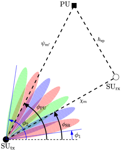
Figure 1: Our opportunistic CR system with an M𝑀M-beam RA at SUtx and omni-directional antennas at SUrx and PU.

II-A Structure of a RA

We consider a RA which can generate M𝑀M beampatterns and these beampatterns cover the angular plane from ϕ1subscriptitalic-ϕ1\phi_{1} to ϕ2subscriptitalic-ϕ2\phi_{2}, i.e., the angular space from ϕ1subscriptitalic-ϕ1\phi_{1} to ϕ2subscriptitalic-ϕ2\phi_{2} is divided into M𝑀M spatial sectors or beams111Throughout this paper, ”sector” and ”beam” are used interchangeably.. One can extend this angular space to cover the entire azimuth plane. The beampattern corresponding to m𝑚m-th beam achieves its maximum at angle κm=2π(m1)Msubscript𝜅𝑚2𝜋𝑚1𝑀\kappa_{m}=\frac{2\pi(m-1)}{M} for m=1,,M𝑚1𝑀m=1,\ldots,M. Fig. 1 shows the beampatterns of a RA with M=7𝑀7M=7 beams. It is noteworthy that the RA can also reconfigure itself to generate an omni-directional pattern. To mathematically model the radiation pattern of beams, we adopt the Gaussian pattern in xy𝑥𝑦x\!-\!y azimuth plane in terms of angle ϕitalic-ϕ\phi given by [29]

p(ϕ)=A1+A0eB((ϕ)ϕ3dB)2,(ϕ)=mod2π(ϕ+π)π,formulae-sequence𝑝italic-ϕsubscript𝐴1subscript𝐴0superscript𝑒𝐵superscriptitalic-ϕsubscriptitalic-ϕ3dB2italic-ϕsubscriptmod2𝜋italic-ϕ𝜋𝜋p(\phi)=\,A_{1}+A_{0}~{}e^{-B\left(\frac{\mathcal{M(\phi)}}{\phi_{\rm{3dB}}}\right)^{2}},\qquad\mathcal{M(\phi)}=\text{mod}_{2\pi}(\phi+\pi)-\pi, (1)

where mod2π(ϕ)subscriptmod2𝜋italic-ϕ\text{mod}_{2\pi}(\phi) denotes the remainder of ϕ2πitalic-ϕ2𝜋\frac{\phi}{2\pi}, B=ln(2)𝐵2B=\ln(2), ϕ3dBsubscriptitalic-ϕ3dB\phi_{\rm{3dB}} is the 3-dB beamwidth, A1subscript𝐴1A_{1} and A0subscript𝐴0A_{0} are two constant antenna parameters. The radiation pattern of m𝑚m-th beam at angle ϕitalic-ϕ\phi is

pm(ϕ)=p(ϕκm),form=1,,M.formulae-sequencesubscript𝑝𝑚italic-ϕ𝑝italic-ϕsubscript𝜅𝑚for𝑚1𝑀p_{m}(\phi)=p(\phi-\kappa_{m}),\qquad\text{for}~{}m=1,\ldots,M. (2)

In this paper, we discuss the received or transmitted signal at m𝑚m-th beam of SUtx. This implies that, during the signal reception or transmission, the SUtx’s antenna parameters are set and tuned such that the beampattern corresponding to m𝑚m-th beam is generated. Given the antenna design, we focus on how the sector-based structure of this RA can be exploited to enhance the system performance of our opportunistic CR system, in which SUtx optimizes its sector-based data communication to SUrx according to the results of its sector-based spectrum sensing.

II-B Description of Our Opportunistic CR System

Our opportunistic CR system model is illustrated in Fig. 1, consisting of a PU and a pair of SUtx and SUrx. We note that PU in our system model can be a primary transmitter or receiver. We assume when PU is active it is engaged in a bidirectional communication with another PU, which is located far from SUtx and hence its activity does not impact our analysis. We assume SUtx is equipped with an M𝑀M-beam RA (for spatial spectrum sensing, channel training and data transmission) with the capability of choosing one out of M𝑀M sectors for its data transmission to SUrx, while SUrx and PU use omni-directional antennas. We assume there is an error-free low-rate feedback channel222Given a low rate feedback, the error-free feedback channel is a reasonable assumption [18]. from SUrx to SUtx, to enable SUtx select the best sector for its data transmission to SUrx, and to adapt its transmit power according to the SUtx–SUrx channel information. The direction (orientation) of PU and SUrx with respect to SUtx are denoted by angles ϕPUsubscriptitalic-ϕPU\phi_{\rm{PU}}, and ϕSRsubscriptitalic-ϕSR\phi_{\rm{SR}}, receptively, where ϕSR,ϕPU(ϕ1,ϕ2)subscriptitalic-ϕSRsubscriptitalic-ϕPUsubscriptitalic-ϕ1subscriptitalic-ϕ2\phi_{\rm{SR}},\phi_{\rm{PU}}\in(\phi_{1},\phi_{2}). Clearly, in our problem SUtx does not know these directions or angles (otherwise, the beam selection at SUtx for data transmission would become trivial).

Let hh, hsssubscriptssh_{\rm{ss}}, hspsubscriptsph_{\rm{sp}} denote the fading coefficients of channels between SUtx and PU, SUtx and SUrx, and SUrx and PU, respectively, when the RA of SUtx is in omni-directional mode. We model these fading coefficients as independent circularly symmetric complex Gaussian random variables. Equivalently, g=|h|2𝑔superscript2g\!=\!|h|^{2}, gss=|hss|2subscript𝑔sssuperscriptsubscriptss2g_{\rm{ss}}\!=\!|h_{\rm{ss}}|^{2} and gsp=|hsp|2subscript𝑔spsuperscriptsubscriptsp2g_{\rm{sp}}\!=\!|h_{\rm{sp}}|^{2} are independent exponentially distributed random variables with mean γ𝛾\gamma, γsssubscript𝛾ss\gamma_{\rm{ss}} and γspsubscript𝛾sp\gamma_{\rm{sp}}, respectively333We note that the distances between users are included in the small scale fading model [31], i.e., the mean values γ,γss,γsp𝛾subscript𝛾sssubscript𝛾sp\gamma,\gamma_{\rm{ss}},\gamma_{\rm{sp}} encompass distance-dependent path loss.. In our problem we assume that SUs and PU cannot cooperate, and hence SUs cannot estimate g𝑔g and gspsubscript𝑔spg_{\rm{sp}}. However, SUtx knows the channel statistics, i.e., the mean values γ𝛾\gamma and γspsubscript𝛾sp\gamma_{\rm{sp}}. Let ψmsubscript𝜓superscript𝑚\psi_{m^{\prime}} and χmsubscript𝜒𝑚\chi_{m} denote the fading coefficients of channel between msuperscript𝑚m^{\prime}-th sector of SUtx and PU, and between m𝑚m-th sector of SUtx and SUrx, respectively, when the RA of SUtx is in directional mode. Using the radiation pattern expression in (2) we can relate ψmsubscript𝜓superscript𝑚\psi_{m^{\prime}} to hh and χmsubscript𝜒𝑚\chi_{m} to hsssubscriptssh_{\rm{ss}} as ψm=hpm(ϕPU)subscript𝜓superscript𝑚subscript𝑝superscript𝑚subscriptitalic-ϕPU\psi_{m^{\prime}}\!=\!h\sqrt{p_{m^{\prime}}(\phi_{\rm{PU}})}, χm=hsspm(ϕSR)subscript𝜒𝑚subscriptsssubscript𝑝𝑚subscriptitalic-ϕSR\chi_{m}\!=\!h_{\rm{ss}}\sqrt{p_{m}(\phi_{\rm{SR}})}. We assume the channel gain νm=|χm|2subscript𝜈𝑚superscriptsubscript𝜒𝑚2\nu_{m}=|\chi_{m}|^{2} is an exponentially distributed random variable with mean αmsubscript𝛼𝑚\alpha_{m}, and SUtx knows αmsubscript𝛼𝑚\alpha_{m}, for all m𝑚m [32, 29]. For the readers’ convenience, we have collected the most commonly used symbols in Table I.

Spatial SpectrumSensingChannelTrainingData TransmissionTfsubscript𝑇fT_{\rm{f}}Tsesubscript𝑇seT_{\rm{se}}Ttrsubscript𝑇trT_{\rm{tr}}Td=TfTseTtrsubscript𝑇dsubscript𝑇fsubscript𝑇sesubscript𝑇trT_{\rm{d}}=T_{\rm{f}}-T_{\rm{se}}-T_{\rm{tr}}
Figure 2: The structure of frame employed by SUtx.
TABLE I: Most commonly used symbols.
Symbol Description
M𝑀M Number of beams
Nsesubscript𝑁seN_{\rm{se}} Number of samples used for spatial spectrum sensing
Ntrsubscript𝑁trN_{\rm{tr}} Number of samples used for channel training
Ptrsubscript𝑃trP_{\rm{tr}} Power of training symbols
ψmsubscript𝜓superscript𝑚\psi_{m^{\prime}} Fading coefficient of channel between msuperscript𝑚m^{\prime}-th beam of
SUtx and PU
χm,χ^m,χ~msubscript𝜒𝑚subscript^𝜒𝑚subscript~𝜒𝑚\chi_{m},\widehat{\chi}_{m},\widetilde{\chi}_{m} Fading coefficient of channel between m𝑚m-th beam of
SUtx and SUrx, LMMSE channel estimate, and its
corresponding estimation error
αm,α^m,α~msubscript𝛼𝑚subscript^𝛼𝑚subscript~𝛼𝑚\alpha_{m},\widehat{\alpha}_{m},\widetilde{\alpha}_{m} Variances of χm,χ^m,χ~msubscript𝜒𝑚subscript^𝜒𝑚subscript~𝜒𝑚\chi_{m},\widehat{\chi}_{m},\widetilde{\chi}_{m}
mPU,mSRsuperscriptsubscript𝑚PUsuperscriptsubscript𝑚SRm_{\rm{PU}}^{*},m_{\rm{SR}}^{*} ​​​​​ Indices of selected beam for PU and SUrx
ν^superscript^𝜈\widehat{\nu}^{*} Channel gain of selected beam for data transmission
from SUtx to SUrx

Suppose, SUs employ a frame with a fixed duration of Tfsubscript𝑇fT_{\rm{f}} seconds, depicted in Fig. 2. We assume the SUtx–SUrx channel remains constant over the frame duration. SUtx first senses the spectrum and monitors PU’s activity. We refer to this period as spatial spectrum sensing phase with a variable duration of Tse=MNseTssubscript𝑇se𝑀subscript𝑁sesubscript𝑇sT_{\rm{se}}=MN_{\rm{se}}T_{\rm{s}} seconds, where Tssubscript𝑇sT_{\rm{s}} is the sampling period and Nsesubscript𝑁seN_{\rm{se}} is the number of collected samples during this phase per beam. Suppose 1subscript1\mathcal{H}_{1} and 0subscript0\mathcal{H}_{0} represent the binary hypotheses of PU being active and inactive, respectively, with prior probabilities Pr{1}=π1Prsubscript1subscript𝜋1\Pr\{\mathcal{H}_{1}\}\!=\!\pi_{1} and Pr{0}=π0Prsubscript0subscript𝜋0\Pr\{\mathcal{H}_{0}\}\!=\!\pi_{0}. SUtx applies a binary detection rule to decide whether or not PU is active. The details of the binary detector are presented in Section III-A. While being in this phase, SUtx determines the beam corresponding to the orientation of PU based on the received signal energy as we describe in Section III-B.

Depending on the outcome of spectrum sensing, SUtx stays in spatial spectrum sensing phase or enters the next phase, which we refer to as channel training phase with a variable duration of Ttr=MNtrTssubscript𝑇tr𝑀subscript𝑁trsubscript𝑇sT_{\rm{tr}}=MN_{\rm{tr}}T_{\rm{s}} seconds. In this phase, SUtx sends Ntrsubscript𝑁trN_{\rm{tr}} training symbols with fixed symbol power Ptrsubscript𝑃trP_{\rm{tr}} per beam to enable channel estimation at SUrx, as we explain in Section IV-A. Based on the results of channel estimation for all beams, SUrx selects the beam with the largest SUtx–SUrx fading gain, as we describe in Section IV-B. This information as well as the corresponding beam index are shared with SUtx via the feedback channel. Next, SUtx enters data transmission phase with a variable duration of Td=TfTseTtrsubscript𝑇dsubscript𝑇fsubscript𝑇sesubscript𝑇trT_{\rm{d}}=T_{\rm{f}}\!-\!T_{\rm{se}}\!-\!T_{\rm{tr}} seconds. During this phase, SUtx sends Nd=Td/Tssubscript𝑁dsubscript𝑇dsubscript𝑇sN_{\rm{d}}=T_{\rm{d}}/T_{\rm{s}} Gaussian data symbols with adaptive symbol power P𝑃P to SUrx over the selected strongest beam. SUtx adapts P𝑃P aiming at maximizing the achievable rates, subject to ATPC and AIC as we describe in Section V. In the following sections, we describe how SUtx operates during spatial spectrum sensing phase, channel training phase, and data transmission phase.

III Spatial Spectrum Sensing Phase

III-A Eigenvalue-Based Detector for Spatial Spectrum Sensing

Let ^1subscript^1\widehat{\mathcal{H}}_{1} and ^0subscript^0\widehat{\mathcal{H}}_{0} denote the detector outcome, i.e., the detector finds PU active (spectrum is sensed busy and occupied) and inactive (spectrum is sensed idle and unoccupied and thus can be used by SUtx for data transmission), respectively. Suppose when PU is active, it transmits signal s(t)𝑠𝑡s(t) with power Ppsubscript𝑃pP_{\rm{p}}. Let ym(n)subscript𝑦𝑚𝑛y_{m}(n) denote the discrete-time representation of received signal at m𝑚m-th sector of SUtx at time instant t=nTs𝑡𝑛subscript𝑇st=nT_{\rm{s}}. We model PU’s transmitted signal s(n)𝑠𝑛s(n) as a zero-mean complex Gaussian random variable with variance Ppsubscript𝑃pP_{\rm{p}} and we assume SUtx knows Ppsubscript𝑃pP_{\rm{p}}. Since SUtx collects Nsesubscript𝑁seN_{\rm{se}} samples per beam during spatial spectrum sensing phase, the hypothesis testing problem at discrete time instant n𝑛n for m𝑚m-th sector is

0::subscript0absent\displaystyle{\cal H}_{0}\!: ym(n)=wm(n),subscript𝑦𝑚𝑛subscript𝑤𝑚𝑛\displaystyle~{}~{}~{}y_{m}(n)=w_{m}(n), (3)
1::subscript1absent\displaystyle{\cal H}_{1}\!: ym(n)=ψm(n)s(n)+wm(n).subscript𝑦𝑚𝑛subscript𝜓𝑚𝑛𝑠𝑛subscript𝑤𝑚𝑛\displaystyle~{}~{}~{}y_{m}(n)=\psi_{m}(n)s(n)+w_{m}(n).

The term wm(n)subscript𝑤𝑚𝑛w_{m}(n) is the additive noise at m𝑚m-th sector of SUtx antenna and is modeled as wm(n)𝒞𝒩(0,σw2)similar-tosubscript𝑤𝑚𝑛𝒞𝒩0superscriptsubscript𝜎w2w_{m}(n)\sim\mathcal{CN}(0,\sigma_{\rm{w}}^{2}). We assume that ψm(n)subscript𝜓𝑚𝑛\psi_{m}(n), s(n)𝑠𝑛s(n) and wm(n)subscript𝑤𝑚𝑛w_{m}(n) are mutually independent random variables. Since SUtx takes samples of the received signal for different sectors sequentially (in different time instants), ψm(n)subscript𝜓𝑚𝑛\psi_{m}(n) and wm(n)subscript𝑤𝑚𝑛w_{m}(n) are independent and thus uncorrelated both in time and space (sector) domains. Under hypothesis 1subscript1\mathcal{H}_{1}, given ψmsubscript𝜓𝑚\psi_{m}, we have ym(n)𝒞𝒩(0,σm2+σw2)similar-tosubscript𝑦𝑚𝑛𝒞𝒩0superscriptsubscript𝜎𝑚2superscriptsubscript𝜎w2y_{m}(n)\sim\mathcal{CN}(0,\sigma_{m}^{2}\!+\!\sigma_{\rm{w}}^{2}) where σm2=|ψm|2Ppsubscriptsuperscript𝜎2𝑚superscriptsubscript𝜓𝑚2subscript𝑃p\sigma^{2}_{m}=|\psi_{m}|^{2}P_{\rm{p}}. Under hypothesis 0subscript0\mathcal{H}_{0}, we have ym(n)𝒞𝒩(0,σw2)similar-tosubscript𝑦𝑚𝑛𝒞𝒩0superscriptsubscript𝜎w2y_{m}(n)\sim\mathcal{CN}(0,\sigma_{\rm{w}}^{2}).

Our proposed binary detector uses all the collected samples from M𝑀M sectors. To facilitate the signal processing needed for the binary detection, we define an M×Nse𝑀subscript𝑁seM\times N_{\rm{se}} sample matrix 𝒁=[𝒛1,,𝒛Nse]𝒁subscript𝒛1subscript𝒛subscript𝑁se\boldsymbol{Z}=[\boldsymbol{z}_{1},\ldots,\boldsymbol{z}_{N_{\rm{se}}}], where the first row of 𝒁𝒁\boldsymbol{Z} is the Nsesubscript𝑁seN_{\rm{se}} samples collected from the first sector, the second row of 𝒁𝒁\boldsymbol{Z} is the Nsesubscript𝑁seN_{\rm{se}} samples collected from the second sector, and so forth. Given our assumptions, the columns of 𝒁𝒁\boldsymbol{Z} are orthogonal under both hypotheses, that is

𝔼{𝒛i𝒛jH\displaystyle\mathbb{E}\big{\{}\boldsymbol{z}_{i}\boldsymbol{z}_{j}^{H} |0}=𝟎,𝔼{𝒛i𝒛jH|1}=𝟎,\displaystyle|\mathcal{H}_{0}\big{\}}=\boldsymbol{0},~{}~{}~{}~{}~{}~{}~{}\mathbb{E}\big{\{}\boldsymbol{z}_{i}\boldsymbol{z}_{j}^{H}|\mathcal{H}_{1}\big{\}}=\boldsymbol{0},
forij,i,j=1,,Nseformulae-sequencefor𝑖𝑗𝑖𝑗1subscript𝑁se\displaystyle\text{for}~{}i\neq j,~{}~{}~{}i,j=1,\ldots,N_{\rm{se}} (4)

where 𝔼{}𝔼\mathbb{E}\{\cdot\} is the statistical expectation operator and have the below covariance matrices

𝚪0=subscript𝚪0absent\displaystyle\boldsymbol{\Gamma}_{0}= 𝔼{𝒛j𝒛jH|0}=σw2𝑰M,𝔼conditional-setsubscript𝒛𝑗subscriptsuperscript𝒛𝐻𝑗subscript0superscriptsubscript𝜎w2subscript𝑰𝑀\displaystyle\mathbb{E}\left\{\boldsymbol{z}_{j}\boldsymbol{z}^{H}_{j}|\mathcal{H}_{0}\right\}=\sigma_{\rm{w}}^{2}\boldsymbol{I}_{M}, (5a)
𝚪1=subscript𝚪1absent\displaystyle\boldsymbol{\Gamma}_{1}= 𝔼{𝒛j𝒛jH|1,𝝍}=Pp𝝍𝝍H+σw2𝑰M,𝔼conditional-setsubscript𝒛𝑗subscriptsuperscript𝒛𝐻𝑗subscript1𝝍subscript𝑃p𝝍superscript𝝍𝐻superscriptsubscript𝜎w2subscript𝑰𝑀\displaystyle\mathbb{E}\left\{\boldsymbol{z}_{j}\boldsymbol{z}^{H}_{j}|\mathcal{H}_{1},\boldsymbol{\psi}\right\}=P_{\rm{p}}\boldsymbol{\psi}\boldsymbol{\psi}^{H}+\sigma_{\rm{w}}^{2}\boldsymbol{I}_{M}, (5b)

where vector 𝝍=[ψ1,ψ2,,ψM]T𝝍superscriptsubscript𝜓1subscript𝜓2subscript𝜓𝑀𝑇\boldsymbol{\psi}=\big{[}\psi_{1},\psi_{2},\ldots,\psi_{M}\big{]}^{T}. Therefore the sample covariance matrix 𝑹^^𝑹\widehat{\boldsymbol{R}} becomes 𝑹^=1Nse𝒁𝒁H.^𝑹1subscript𝑁se𝒁superscript𝒁𝐻\widehat{\boldsymbol{R}}=\frac{1}{N_{\rm{se}}}\boldsymbol{Z}\boldsymbol{Z}^{H}.

Let f(𝐙|0)𝑓conditional𝐙subscript0f({\bf Z}|{\cal H}_{0}) and f(𝐙|1,𝝍)𝑓conditional𝐙subscript1𝝍f({\bf Z}|{\cal H}_{1},\boldsymbol{\psi}) denote the probability distribution function (pdf) of 𝐙𝐙{\bf Z} under 0subscript0{\cal H}_{0} and 1subscript1{\cal H}_{1} (given 𝝍𝝍\boldsymbol{\psi}), respectively. These pdf expressions are

f(𝐙|0)=𝑓conditional𝐙subscript0absent\displaystyle f({\bf Z}|{\cal H}_{0})\!=\, 1(πσw2)Neqexp{tr(𝐙𝐙H)σw2},1superscript𝜋superscriptsubscript𝜎w2subscript𝑁eqtrsuperscript𝐙𝐙𝐻superscriptsubscript𝜎w2\displaystyle{1\over(\pi\sigma_{\rm{w}}^{2})^{N_{\rm{eq}}}}\exp\left\{\!{{{\rm tr}({\bf ZZ}^{H})}\over{-\sigma_{\rm{w}}^{2}}}\!\right\}, (6a)
f(𝐙|1,𝝍)=𝑓conditional𝐙subscript1𝝍absent\displaystyle f({\bf Z}|{\cal H}_{1},\boldsymbol{\psi})\!=\, 1πNeqdet(𝚪𝟏)Nseexp{tr(𝚪11𝐙𝐙H)σw2},1superscript𝜋subscript𝑁eqsuperscriptsubscript𝚪1subscript𝑁setrsuperscriptsubscript𝚪11superscript𝐙𝐙𝐻superscriptsubscript𝜎w2\displaystyle{1\over{\pi^{N_{\rm{eq}}}\det({\bf\Gamma_{1}})^{N_{\rm{se}}}}}\exp\!\left\{\!{{{\rm tr}({\bf\Gamma}_{1}^{-1}{\bf ZZ}^{H})}\over{-\sigma_{\rm{w}}^{2}}}\!\right\}, (6b)

where Neq=MNsesubscript𝑁eq𝑀subscript𝑁seN_{\rm{eq}}=MN_{\rm{se}}. The optimal detector would compare the logarithm of likelihood ratio (LLR) against a threshold η0subscript𝜂0\eta_{0} to detect the PU’s activity as below

LLR=lnf(𝐙|1,𝝍)f(𝐙|0)^1^0η0.LLR𝑓conditional𝐙subscript1𝝍𝑓conditional𝐙subscript0greater-than-or-equals-or-less-thanmatrixsubscript^1subscript^0subscript𝜂0\text{LLR}=\ln\frac{f({\bf Z}|{\cal H}_{1},\boldsymbol{\psi})}{f({\bf Z}|{\cal H}_{0})}\gtreqless\begin{matrix}\widehat{\cal H}_{1}\cr\widehat{\cal H}_{0}\end{matrix}\eta_{0}. (7)

In the absence of the knowledge of the fading coefficients vector 𝝍𝝍\boldsymbol{\psi}, SUtx obtains the generalized likelihood ratio test (GLRT) [33, 34, 35, 36, 37] which uses the maximum likelihood (ML) estimate of 𝝍𝝍\boldsymbol{\psi} under 1subscript1\mathcal{H}_{1}. Let 1(𝐙)=lnf(𝐙|1,𝝍)subscript1𝐙𝑓conditional𝐙subscript1𝝍\mathcal{L}_{1}({\bf Z})=\ln f({\bf Z}|{\cal H}_{1},\boldsymbol{\psi}). To find the maximum of 1(𝐙)subscript1𝐙\mathcal{L}_{1}({\bf Z}) with respect to 𝝍𝝍\boldsymbol{\psi}, we take the derivative of 1(𝐙)subscript1𝐙\mathcal{L}_{1}({\bf Z}) with respect to 𝝍𝝍\boldsymbol{\psi} and solve 𝝍1(𝐙)=𝟎𝝍subscript1𝐙0\frac{\partial}{\partial\boldsymbol{\psi}}\mathcal{L}_{1}({\bf Z})={\bf 0} for 𝝍𝝍\boldsymbol{\psi}. The obtained solution is the ML estimate of 𝝍𝝍\boldsymbol{\psi}. Substituting this solution into (7) and after some mathematical manipulation, we reach the following decision rule T=λmaxσw2^1^0η𝑇subscript𝜆maxsuperscriptsubscript𝜎w2greater-than-or-equals-or-less-thanmatrixsubscript^1subscript^0𝜂T=\frac{\lambda_{\text{max}}}{\sigma_{\rm{w}}^{2}}\gtreqless{\small\begin{matrix}\widehat{\cal H}_{1}\cr\widehat{\cal H}_{0}\end{matrix}}\eta [36], where T𝑇T is the test statistics, λmaxsubscript𝜆max\lambda_{\text{max}} is the maximum eigenvalue of 𝑹^^𝑹\widehat{\boldsymbol{R}}, and η𝜂\eta is the threshold. For large Nsesubscript𝑁seN_{\rm{se}}, T𝑇T under 0subscript0{\cal H}_{0} is distributed as Tracy-Widom distribution of order 2 [36, Lemma 1] and the probability of false alarm Pfa=Pr(^1|0)=Pr(T>η|0)subscript𝑃faPrconditionalsubscript^1subscript0Pr𝑇conditional𝜂subscript0P_{\rm{fa}}=\Pr(\widehat{\cal H}_{1}|{\cal H}_{0})=\Pr(T>\eta|{\cal H}_{0}) is

Pfa=1FTW2(ηθsenσsen),subscript𝑃fa1subscript𝐹TW2𝜂subscript𝜃sensubscript𝜎senP_{\rm{fa}}=1-F_{\text{TW2}}\left(\frac{\eta\!-\!\theta_{\rm{sen}}}{\sigma_{\rm{sen}}}\right), (8)

where FTW2()subscript𝐹TW2F_{\text{TW2}}(\cdot) is the commutative distribution function (CDF) of Tracy-Widom distribution of order 2 and θsensubscript𝜃sen\theta_{\rm{sen}} and σsensubscript𝜎sen\sigma_{\rm{sen}} in (8) are given below

θsen=(1+MNse)2,subscript𝜃sensuperscript1𝑀subscript𝑁se2\displaystyle\theta_{\rm{sen}}=\bigg{(}1+\sqrt{\frac{M}{N_{\rm{se}}}}\bigg{)}^{2}, (9a)
σsen=1Nsesubscript𝜎sen1subscript𝑁se\displaystyle\sigma_{\rm{sen}}=\frac{1}{\sqrt{N_{\rm{se}}}} (1+MNse)(1Nse+1M)13.1𝑀subscript𝑁sesuperscript1subscript𝑁se1𝑀13\displaystyle\bigg{(}1\!+\!\sqrt{\frac{M}{N_{\rm{se}}}}\bigg{)}\bigg{(}\frac{1}{\sqrt{N_{\rm{se}}}}\!+\!\frac{1}{\sqrt{M}}\bigg{)}^{\frac{1}{3}}. (9b)

For large Nsesubscript𝑁seN_{\rm{se}}, T𝑇T under 1subscript1{\cal H}_{1} is Gaussian distributed [36, Lemma 2] and the probability of detection Pd=Pr(^1|1)=Pr(T>η|1)subscript𝑃dPrconditionalsubscript^1subscript1Pr𝑇conditional𝜂subscript1P_{\rm{d}}=\Pr(\widehat{\cal H}_{1}|{\cal H}_{1})=\Pr(T>\eta|{\cal H}_{1}) is [37, 36]

Pd=Q(ηNse1+δsenM1δsenNseNse),subscript𝑃d𝑄𝜂subscript𝑁se1subscript𝛿sen𝑀1subscript𝛿sensubscript𝑁sesubscript𝑁seP_{\rm{d}}=Q\left(\frac{\eta\sqrt{N_{\rm{se}}}}{1\!+\!\delta_{\rm{sen}}}\!-\!\frac{M\!-\!1}{\delta_{\rm{sen}}\sqrt{N_{\rm{se}}}}\!-\!\sqrt{N_{\rm{se}}}\right), (10)

where δsen=Pp𝝍2σw2subscript𝛿sensubscript𝑃psuperscriptnorm𝝍2superscriptsubscript𝜎w2\delta_{\rm{sen}}=\frac{P_{\rm{p}}\|\boldsymbol{\psi}\|^{2}}{\sigma_{\rm{w}}^{2}}. The average detection probability P¯dsubscript¯𝑃d\overline{P}_{\rm{d}} can be computed by averaging (10) over vector 𝝍𝝍\boldsymbol{\psi}, P¯d=𝔼𝝍{Pd}subscript¯𝑃dsubscript𝔼𝝍subscript𝑃d\overline{P}_{\rm{d}}=\mathbb{E}_{\boldsymbol{\psi}}\{P_{\rm{d}}\}. For a given P¯dsubscript¯𝑃d\overline{P}_{\rm{d}}, we can numerically find η𝜂\eta and obtain P¯fasubscript¯𝑃fa\overline{P}_{\rm{fa}} using (8). We can also compute the probabilities of events ^0subscript^0\widehat{\mathcal{H}}_{0} and ^1subscript^1\widehat{\mathcal{H}}_{1} as π^0=Pr{^0}=β0+β1subscript^𝜋0Prsubscript^0subscript𝛽0subscript𝛽1\widehat{\pi}_{0}\!=\!\Pr\{\widehat{\mathcal{H}}_{0}\}=\beta_{0}+\beta_{1} and π^1=Pr{^1}=1π^0subscript^𝜋1Prsubscript^11subscript^𝜋0\widehat{\pi}_{1}\!=\!\Pr\{\widehat{\mathcal{H}}_{1}\}=1-\widehat{\pi}_{0}, respectively, where

β0=Pr{0,^0}=π0(1P¯fa),subscript𝛽0Prsubscript0subscript^0subscript𝜋01subscript¯𝑃fa\displaystyle\beta_{0}=\Pr\{\mathcal{H}_{0},\widehat{\mathcal{H}}_{0}\}=\pi_{0}(1-\overline{P}_{\rm{fa}}), (11a)
β1=Pr{1,^0}=π1(1P¯d).subscript𝛽1Prsubscript1subscript^0subscript𝜋11subscript¯𝑃d\displaystyle\beta_{1}=\Pr\{\mathcal{H}_{1},\widehat{\mathcal{H}}_{0}\}=\pi_{1}(1-\overline{P}_{\rm{d}}). (11b)

III-B Determining the Beam Corresponding to PU Direction

During spatial spectrum sensing phase when the spectrum is sensed busy, SUtx determines the beam corresponding to the direction of PU based on the received signal energy. Let εmsubscript𝜀𝑚\varepsilon_{m} be the energy of received signal at m𝑚m-th beam. We have

εm=1Nsen=1+(m1)NsemNse|ym(n)|2.subscript𝜀𝑚1subscript𝑁sesuperscriptsubscript𝑛1𝑚1subscript𝑁se𝑚subscript𝑁sesuperscriptsubscript𝑦𝑚𝑛2\varepsilon_{m}=\frac{1}{N_{\rm{se}}}\sum_{n=1+(m\!-\!1)N_{\rm{se}}}^{mN_{\rm{se}}}\!\!\!\big{|}y_{m}(n)\big{|}^{2}. (12)

SUtx determines the beam with the largest amount of received energy mPU=argmax{εm}superscriptsubscript𝑚PUsubscript𝜀𝑚m_{\rm{PU}}^{*}=\arg\max\{\varepsilon_{m}\} among all beams. For large Nsesubscript𝑁seN_{\rm{se}}, we invoke central limit theorem (CLT) to approximate εmsubscript𝜀𝑚\varepsilon_{m}’s as Gaussian random variables under both hypotheses. Thus, under 0subscript0{\cal H}_{0} we approximate εmsubscript𝜀𝑚\varepsilon_{m} as a Gaussian with distribution εm𝒩(σw2,σw4/Nse)similar-tosubscript𝜀𝑚𝒩superscriptsubscript𝜎w2superscriptsubscript𝜎w4subscript𝑁se\varepsilon_{m}\sim\mathcal{N}(\sigma_{\rm{w}}^{2},\sigma_{\rm{w}}^{4}/N_{\rm{se}}). Similarly, under 1subscript1{\cal H}_{1}, given ϕPUsubscriptitalic-ϕPU\phi_{\rm{PU}} we approximate εmsubscript𝜀𝑚\varepsilon_{m} as another Gaussian with distribution εm𝒩(ϱm,σεm|12)similar-tosubscript𝜀𝑚𝒩subscriptitalic-ϱ𝑚subscriptsuperscript𝜎2conditionalsubscript𝜀𝑚subscript1\varepsilon_{m}\sim\mathcal{N}(\varrho_{m},\sigma^{2}_{\varepsilon_{m}|{\cal H}_{1}}), where the mean ϱm=γPppm(ϕPU)+σw2subscriptitalic-ϱ𝑚𝛾subscript𝑃psubscript𝑝𝑚subscriptitalic-ϕPUsuperscriptsubscript𝜎w2\varrho_{m}=\gamma P_{\rm{p}}\,p_{m}(\phi_{\rm{PU}})+\sigma_{\rm{w}}^{2}, and the variance σεm|12subscriptsuperscript𝜎2conditionalsubscript𝜀𝑚subscript1\sigma^{2}_{\varepsilon_{m}|{\cal H}_{1}} is given below

σεm|12=1Nse[σw4+3Pp2γ2pm2(ϕPU)+2σw2Ppγpm(ϕPU)].subscriptsuperscript𝜎2conditionalsubscript𝜀𝑚subscript11subscript𝑁sedelimited-[]superscriptsubscript𝜎w43superscriptsubscript𝑃p2superscript𝛾2superscriptsubscript𝑝𝑚2subscriptitalic-ϕPU2superscriptsubscript𝜎w2subscript𝑃p𝛾subscript𝑝𝑚subscriptitalic-ϕPU\sigma^{2}_{\varepsilon_{m}|{\cal H}_{1}}=\frac{1}{N_{\rm{se}}}\Big{[}\sigma_{\rm{w}}^{4}+3P_{\rm{p}}^{2}\gamma^{2}\,p_{m}^{2}(\phi_{\rm{PU}})+2\sigma_{\rm{w}}^{2}P_{\rm{p}}\gamma\,p_{m}(\phi_{\rm{PU}})\Big{]}. (13)

We note that, there is a non-zero error probability when SUtx determines the beam index mPUsuperscriptsubscript𝑚PUm_{\rm{PU}}^{*}, i.e., it is possible that mPUsuperscriptsubscript𝑚PUm_{\rm{PU}}^{*} is not the true beam index corresponding to PU direction.

Let Δ¯i,msubscript¯Δ𝑖𝑚\overline{\Delta}_{i,m} represent the average error probability of finding the sector index corresponding to PU direction, i.e., the probability that mPU=isuperscriptsubscript𝑚PU𝑖m_{\rm{PU}}^{*}=i while the true PU direction lies in the angular domain of m𝑚m-th sector, ϕPUΦm=[2π(m3/2)M,2π(m1/2)M)subscriptitalic-ϕPUsubscriptΦ𝑚2𝜋𝑚32𝑀2𝜋𝑚12𝑀\phi_{\rm{PU}}\in\Phi_{m}=\big{[}\frac{2\pi(m-3/2)}{M},\frac{2\pi(m-1/2)}{M}\big{)}, for im,i,m=1,,Mformulae-sequence𝑖𝑚𝑖𝑚1𝑀i\neq m,i,m=1,\ldots,M. To find Δ¯i,msubscript¯Δ𝑖𝑚\overline{\Delta}_{i,m} we start with finding Δi=Pr{mPU=i|ϕPU,^1}subscriptΔ𝑖Prsuperscriptsubscript𝑚PUconditional𝑖subscriptitalic-ϕPUsubscript^1\Delta_{i}=\Pr\{m_{\rm{PU}}^{*}\!=\!i|\phi_{\rm{PU}},\widehat{\cal H}_{1}\}, which is the probability that the index of selected sector is i𝑖i, given ϕPUsubscriptitalic-ϕPU\phi_{\rm{PU}} and ^1subscript^1\widehat{\cal H}_{1} (the binary detector in Section III-A finds PU active). Note that under both hypotheses, εmsubscript𝜀𝑚\varepsilon_{m}’s are independent. Also, under 0subscript0{\cal H}_{0}, εmsubscript𝜀𝑚\varepsilon_{m}’s are identically distributed. Therefore, we have

Δi=subscriptΔ𝑖absent\displaystyle\Delta_{i}= Pr{εi>εmm,mi|ϕPU,^1}Prconditionalfor-all𝑚𝑚𝑖subscript𝜀𝑖subscript𝜀𝑚subscriptitalic-ϕPUsubscript^1\displaystyle\,\Pr\Big{\{}\underset{\forall m,\,m\neq i}{\varepsilon_{i}>\varepsilon_{m}}\,\big{|}\phi_{\rm{PU}},\widehat{\cal H}_{1}\Big{\}}
=\displaystyle= ς10fεi|1(y|ϕPU)m=1miMFεm|1(y|ϕPU)dysubscript𝜍1superscriptsubscript0subscript𝑓conditionalsubscript𝜀𝑖subscript1conditional𝑦subscriptitalic-ϕPUsuperscriptsubscriptproduct𝑚𝑖𝑚1𝑀subscript𝐹conditionalsubscript𝜀𝑚subscript1conditional𝑦subscriptitalic-ϕPU𝑑𝑦\displaystyle\,\varsigma_{1}\int_{0}^{\infty}f_{\varepsilon_{i}|{\cal H}_{1}}\big{(}y|\phi_{\rm{PU}}\big{)}\!\prod_{\underset{m\neq i}{m=1}}^{M}\!F_{\varepsilon_{m}|{\cal H}_{1}}\big{(}y|\phi_{\rm{PU}}\big{)}dy
+\displaystyle+ ς00fεm|0(y)Fεm|0M1(y)𝑑ysubscript𝜍0superscriptsubscript0subscript𝑓conditionalsubscript𝜀𝑚subscript0𝑦subscriptsuperscript𝐹𝑀1conditionalsubscript𝜀𝑚subscript0𝑦differential-d𝑦\displaystyle\,\varsigma_{0}\int_{0}^{\infty}f_{\varepsilon_{m}|{\cal H}_{0}}\big{(}y\big{)}F^{M-1}_{\varepsilon_{m}|{\cal H}_{0}}\big{(}y\big{)}dy (14)

where fεm|(x)subscript𝑓conditionalsubscript𝜀𝑚subscript𝑥f_{\varepsilon_{m}|{\cal H}_{\ell}}(x) and Fεm|(x)subscript𝐹conditionalsubscript𝜀𝑚subscript𝑥F_{\varepsilon_{m}|{\cal H}_{\ell}}(x) are the pdf and CDF expressions of εmsubscript𝜀𝑚\varepsilon_{m} under ,=0,1formulae-sequencesubscript01{\cal H}_{\ell},\ell=0,1 and

ς0=Pr{0|^1}=π0P¯faπ^1,subscript𝜍0Prconditionalsubscript0subscript^1subscript𝜋0subscript¯𝑃fasubscript^𝜋1\displaystyle\varsigma_{0}=\Pr\{\mathcal{H}_{0}|\widehat{\mathcal{H}}_{1}\}={\pi_{0}\overline{P}_{\rm{fa}}\over\widehat{\pi}_{1}}, (15a)
ς1=Pr{1|^1}=π1P¯dπ^1.subscript𝜍1Prconditionalsubscript1subscript^1subscript𝜋1subscript¯𝑃dsubscript^𝜋1\displaystyle\varsigma_{1}=\Pr\{\mathcal{H}_{1}|\widehat{\mathcal{H}}_{1}\}={\pi_{1}\overline{P}_{\rm{d}}\over\widehat{\pi}_{1}}. (15b)

Using ΔisubscriptΔ𝑖\Delta_{i}, we find Δ¯i,msubscript¯Δ𝑖𝑚\overline{\Delta}_{i,m} as the following

Δ¯i,m=ϕPUΦmΔiPr{ϕPUΦm}𝑑ϕPU.subscript¯Δ𝑖𝑚subscriptsubscriptitalic-ϕPUsubscriptΦ𝑚subscriptΔ𝑖Prsubscriptitalic-ϕPUsubscriptΦ𝑚differential-dsubscriptitalic-ϕPU\overline{\Delta}_{i,m}=\int\nolimits_{\phi_{\rm{PU}}\in\Phi_{m}}\!\!\!\!\!\Delta_{i}\Pr\!\big{\{}\phi_{\rm{PU}}\!\in\!\Phi_{m}\big{\}}~{}d\phi_{\rm{PU}}. (16)

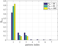
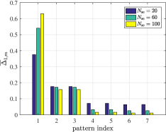
Note that Δ¯i,isubscript¯Δ𝑖𝑖\overline{\Delta}_{i,i} is the probability of selecting the correct beam and Δ¯i,msubscript¯Δ𝑖𝑚\overline{\Delta}_{i,m} for im𝑖𝑚i\neq m is the probability of selecting the incorrect beam, leading to error probability in beam selection. The average error probability Δ¯1,msubscript¯Δ1𝑚\overline{\Delta}_{1,m} versus the index beam m𝑚m is shown in Figs. 3(a) and 3(b) for SNRPU=γPp/σw2=0,5formulae-sequencesubscriptSNRPU𝛾subscript𝑃psuperscriptsubscript𝜎w205\text{SNR}_{\rm{PU}}\!=\!\gamma P_{\rm{p}}/\sigma_{\rm{w}}^{2}\!=\!0,-5 dB. As expected, Δ¯1,1subscript¯Δ11\overline{\Delta}_{1,1} increases and Δ¯1,m,m1subscript¯Δ1𝑚𝑚1\overline{\Delta}_{1,m},m\neq 1 decreases as Nsesubscript𝑁seN_{\rm{se}} increases.

Refer to caption
(a)
Refer to caption
(b)
Figure 3: Δ¯1,msubscript¯Δ1𝑚\overline{\Delta}_{1,m} versus the index beam m𝑚m for ϕ3dB=20°subscriptitalic-ϕ3dBsuperscript20°\phi_{\rm{3dB}}\!=\!20^{\degree} (a) SNRPU=0subscriptSNRPU0\text{SNR}_{\rm{PU}}\!=\!0 dB, (b) SNRPU=5subscriptSNRPU5\text{SNR}_{\rm{PU}}\!=\!-5 dB.

IV Channel Training Phase

IV-A Channel Estimation at SUrx

During this phase, SUtx sends the training vector 𝒙tsubscript𝒙𝑡\boldsymbol{x}_{t} over all beams to enable channel estimation at SUrx. Without loss of generality, we assume 𝒙t=Ptr 1subscript𝒙𝑡subscript𝑃tr1\boldsymbol{x}_{t}=\sqrt{P_{\rm{tr}}}\,\boldsymbol{1}, where 𝟏1\boldsymbol{1} is an Ntr×1subscript𝑁tr1N_{\rm{tr}}\times 1 all-ones vector and Ptrsubscript𝑃trP_{\rm{tr}} is given. Let 𝒓m=[rm(1),,rm(Ntr)]Tsubscript𝒓𝑚superscriptsubscript𝑟𝑚1subscript𝑟𝑚subscript𝑁tr𝑇\boldsymbol{r}_{m}=\big{[}r_{m}(1),\ldots,r_{m}(N_{\rm{tr}})\big{]}^{T} denote the discrete-time representation of received training symbols at SUrx from m𝑚m-th sector of SUtx. We note that SUtx enters this phase when the outcome of the binary detector in Section III-A is ^0subscript^0\widehat{\cal H}_{0}. Due to error in spatial spectrum sensing, we need to differentiate the signal model for rmsubscript𝑟𝑚r_{m} under 0subscript0{\cal H}_{0} and 1subscript1{\cal H}_{1}. Assuming the fading coefficient χmsubscript𝜒𝑚\chi_{m} is unchanged during the frame, we have

0,^0::subscript0subscript^0absent\displaystyle{\cal H}_{0},\widehat{\cal H}_{0}\!: rm(n)=χmPtr+qm(n),subscript𝑟𝑚𝑛subscript𝜒𝑚subscript𝑃trsubscript𝑞𝑚𝑛\displaystyle~{}~{}~{}r_{m}(n)=\chi_{m}\,\sqrt{P_{\rm{tr}}}+{q_{m}(n)}, (17)
1,^0::subscript1subscript^0absent\displaystyle{\cal H}_{1},\widehat{\cal H}_{0}\!: rm(n)=χmPtr+hsp(n)s(n)+qm(n),subscript𝑟𝑚𝑛subscript𝜒𝑚subscript𝑃trsubscriptsp𝑛𝑠𝑛subscript𝑞𝑚𝑛\displaystyle~{}~{}~{}r_{m}(n)=\chi_{m}\,\sqrt{P_{\rm{tr}}}+{h_{\rm{sp}}(n)}\,s(n)+{q_{m}(n)},

where qm(n)subscript𝑞𝑚𝑛q_{m}(n) is the additive noise at SUrx antenna and is modeled as qm(n)𝒞𝒩(0,σq2)similar-tosubscript𝑞𝑚𝑛𝒞𝒩0superscriptsubscript𝜎q2q_{m}(n)\sim{\cal CN}\big{(}0,\sigma_{\rm{q}}^{2}\big{)}. The linear minimum mean square error (LMMSE) estimation of fading coefficient χmsubscript𝜒𝑚{\chi}_{m} when the spectrum sensing result is ^0subscript^0\widehat{\cal H}_{0} can be obtained as [38]

χ^m=subscript^𝜒𝑚absent\displaystyle\widehat{\chi}_{m}=\, Cχm𝒓mC𝒓m1𝒓m,subscript𝐶subscript𝜒𝑚subscript𝒓𝑚subscriptsuperscript𝐶1subscript𝒓𝑚subscript𝒓𝑚\displaystyle C_{\chi_{m}\boldsymbol{r}_{m}}C^{-1}_{\boldsymbol{r}_{m}}\,\boldsymbol{r}_{m}, (18a)
Cχm𝒓m=subscript𝐶subscript𝜒𝑚subscript𝒓𝑚absent\displaystyle C_{\chi_{m}\boldsymbol{r}_{m}}=\, 𝔼{χm𝒓mH|^0}=Ptrαm 1,𝔼conditional-setsubscript𝜒𝑚subscriptsuperscript𝒓𝐻𝑚subscript^0subscript𝑃trsubscript𝛼𝑚1\displaystyle\mathbb{E}\{\chi_{m}\boldsymbol{r}^{H}_{m}|\widehat{\cal H}_{0}\}=\sqrt{P_{\rm{tr}}}\,\alpha_{m}\,\boldsymbol{1}, (18b)
C𝒓m=subscript𝐶subscript𝒓𝑚absent\displaystyle C_{\boldsymbol{r}_{m}}=\, 𝔼{𝒓m𝒓mH|^0}=ω0𝔼{𝒓m𝒓mH|0,^0}𝔼conditional-setsubscript𝒓𝑚subscriptsuperscript𝒓𝐻𝑚subscript^0subscript𝜔0𝔼conditional-setsubscript𝒓𝑚subscriptsuperscript𝒓𝐻𝑚subscript0subscript^0\displaystyle\mathbb{E}\big{\{}\boldsymbol{r}_{m}\boldsymbol{r}^{H}_{m}|\widehat{\cal H}_{0}\big{\}}=\omega_{0}\,\mathbb{E}\big{\{}\boldsymbol{r}_{m}\boldsymbol{r}^{H}_{m}|{\cal H}_{0},\widehat{\cal H}_{0}\big{\}}
+ω1𝔼{𝒓m𝒓mH|1,^0},subscript𝜔1𝔼conditional-setsubscript𝒓𝑚subscriptsuperscript𝒓𝐻𝑚subscript1subscript^0\displaystyle\qquad\qquad\qquad~{}+\omega_{1}\,\mathbb{E}\big{\{}\boldsymbol{r}_{m}\boldsymbol{r}^{H}_{m}|{\cal H}_{1},\widehat{\cal H}_{0}\big{\}}, (18c)

where

ω0=Pr{0|^0}=π0(1P¯fa)π^0=β0π^0,subscript𝜔0Prconditionalsubscript0subscript^0subscript𝜋01subscript¯𝑃fasubscript^𝜋0subscript𝛽0subscript^𝜋0\displaystyle\omega_{0}=\Pr\{\mathcal{H}_{0}|\widehat{\mathcal{H}}_{0}\}={\pi_{0}(1-\overline{P}_{\rm{fa}})\over\widehat{\pi}_{0}}={\beta_{0}\over\widehat{\pi}_{0}}, (19a)
ω1=Pr{1|^0}=π1(1P¯d)π^0=β1π^0.subscript𝜔1Prconditionalsubscript1subscript^0subscript𝜋11subscript¯𝑃dsubscript^𝜋0subscript𝛽1subscript^𝜋0\displaystyle\omega_{1}=\Pr\{\mathcal{H}_{1}|\widehat{\mathcal{H}}_{0}\}={\pi_{1}(1-\overline{P}_{\rm{d}})\over\widehat{\pi}_{0}}={\beta_{1}\over\widehat{\pi}_{0}}. (19b)

Finally, the LMMSE estimation of χmsubscript𝜒𝑚{\chi}_{m} when the spectrum sensing result is ^0subscript^0\widehat{\cal H}_{0}, given in (18a), reduces to

χ^m=αmPtrαmPtrNtr+σw2+ω1σp2n=1Ntrrm(n),subscript^𝜒𝑚subscript𝛼𝑚subscript𝑃trsubscript𝛼𝑚subscript𝑃trsubscript𝑁trsuperscriptsubscript𝜎w2subscript𝜔1superscriptsubscript𝜎p2superscriptsubscript𝑛1subscript𝑁trsubscript𝑟𝑚𝑛\widehat{\chi}_{m}=\frac{\alpha_{m}\sqrt{P_{\rm{tr}}}}{\alpha_{m}P_{\rm{tr}}N_{\rm{tr}}+{\sigma_{\rm{w}}^{2}}+\omega_{1}{\sigma_{\rm{p}}^{2}}}\sum_{n=1}^{N_{\rm{tr}}}r_{m}(n), (20)

where σp2=Ppγspsuperscriptsubscript𝜎p2subscript𝑃psubscript𝛾sp\sigma_{\rm{p}}^{2}=P_{\rm{p}}\gamma_{\rm{sp}}. The estimation error is χ~m=χmχ^msubscript~𝜒𝑚subscript𝜒𝑚subscript^𝜒𝑚\widetilde{\chi}_{m}=\chi_{m}-\widehat{\chi}_{m} where χ^msubscript^𝜒𝑚\widehat{\chi}_{m} and χ~msubscript~𝜒𝑚\widetilde{\chi}_{m} are orthogonal random variables [38], and χ^msubscript^𝜒𝑚\widehat{\chi}_{m} and χ~msubscript~𝜒𝑚\widetilde{\chi}_{m} are zero mean. Approximating hsp(n)s(n)subscriptsp𝑛𝑠𝑛h_{\rm{sp}}(n)s(n) as a zero-mean Gaussian random variable with variance σp2superscriptsubscript𝜎p2{\sigma_{\rm{p}}^{2}}, we find that the estimate χ^msubscript^𝜒𝑚\widehat{\chi}_{m} is distributed as a Gaussian mixture random variable [16, 39]. Let α^msubscript^𝛼𝑚\widehat{\alpha}_{m} and α~msubscript~𝛼𝑚\widetilde{\alpha}_{m}, represent the variances of χ^msubscript^𝜒𝑚\widehat{\chi}_{m} and χ~msubscript~𝜒𝑚\widetilde{\chi}_{m}, respectively. Also, Let α^m0subscriptsuperscript^𝛼0𝑚\widehat{\alpha}^{0}_{m} and α^m1subscriptsuperscript^𝛼1𝑚\widehat{\alpha}^{1}_{m} represent the variances of χ^msubscript^𝜒𝑚\widehat{\chi}_{m} under 0subscript0{\cal H}_{0} and 1subscript1{\cal H}_{1}, respectively. We have

α^m0=subscriptsuperscript^𝛼0𝑚absent\displaystyle\widehat{\alpha}^{0}_{m}\!=\! 𝕍𝔸{χ^m|0,^0}=αm2PtrNtr(αmPtrNtr+σw2)(αmPtrNtr+σw2+ω1σp2)2,𝕍𝔸conditional-setsubscript^𝜒𝑚subscript0subscript^0superscriptsubscript𝛼𝑚2subscript𝑃trsubscript𝑁trsubscript𝛼𝑚subscript𝑃trsubscript𝑁trsuperscriptsubscript𝜎w2superscriptsubscript𝛼𝑚subscript𝑃trsubscript𝑁trsuperscriptsubscript𝜎w2subscript𝜔1superscriptsubscript𝜎p22\displaystyle\,\mathbb{VAR}\{\widehat{\chi}_{m}|{\cal H}_{0},{\widehat{\cal H}_{0}}\}\!=\!\frac{\alpha_{m}^{2}P_{\rm{tr}}N_{\rm{tr}}\big{(}\alpha_{m}P_{\rm{tr}}N_{\rm{tr}}\!+\!{\sigma_{\rm{w}}^{2}}\big{)}}{\big{(}\alpha_{m}P_{\rm{tr}}N_{\rm{tr}}\!+\!{\sigma_{\rm{w}}^{2}}\!+\!\omega_{1}{\sigma_{\rm{p}}^{2}}\big{)}^{2}}, (21a)
α^m1=subscriptsuperscript^𝛼1𝑚absent\displaystyle\widehat{\alpha}^{1}_{m}\!=\! 𝕍𝔸{χ^m|1,^0}=αm2PtrNtr(αmPtrNtr+σw2+σp2)(αmPtrNtr+σw2+ω1σp2)2.𝕍𝔸conditional-setsubscript^𝜒𝑚subscript1subscript^0superscriptsubscript𝛼𝑚2subscript𝑃trsubscript𝑁trsubscript𝛼𝑚subscript𝑃trsubscript𝑁trsuperscriptsubscript𝜎w2superscriptsubscript𝜎p2superscriptsubscript𝛼𝑚subscript𝑃trsubscript𝑁trsuperscriptsubscript𝜎w2subscript𝜔1superscriptsubscript𝜎p22\displaystyle\,\mathbb{VAR}\{\widehat{\chi}_{m}|{\cal H}_{1},{\widehat{\cal H}_{0}}\}\!=\!\frac{\alpha_{m}^{2}P_{\rm{tr}}N_{\rm{tr}}\big{(}\alpha_{m}P_{\rm{tr}}N_{\rm{tr}}\!+\!{\sigma_{\rm{w}}^{2}}\!+\!{\sigma_{\rm{p}}^{2}}\big{)}}{\big{(}\alpha_{m}P_{\rm{tr}}N_{\rm{tr}}+{\sigma_{\rm{w}}^{2}}\!+\!\omega_{1}{\sigma_{\rm{p}}^{2}}\big{)}^{2}}. (21b)

Therefore, α^m=ω0α^m0+ω1α^m1subscript^𝛼𝑚subscript𝜔0subscriptsuperscript^𝛼0𝑚subscript𝜔1subscriptsuperscript^𝛼1𝑚\widehat{\alpha}_{m}={\omega_{0}}\,\widehat{\alpha}^{0}_{m}+{\omega_{1}}\,\widehat{\alpha}^{1}_{m}. Also, let α~m0subscriptsuperscript~𝛼0𝑚\widetilde{\alpha}^{0}_{m} and α~m1subscriptsuperscript~𝛼1𝑚\widetilde{\alpha}^{1}_{m} indicate the variances of χ~msubscript~𝜒𝑚\widetilde{\chi}_{m} under 0subscript0{\cal H}_{0} and 1subscript1{\cal H}_{1}, respectively. We have

α~m0=subscriptsuperscript~𝛼0𝑚absent\displaystyle\widetilde{\alpha}^{0}_{m}= 𝕍𝔸{χ~m|0,^0}=αmα^m0,𝕍𝔸conditional-setsubscript~𝜒𝑚subscript0subscript^0subscript𝛼𝑚subscriptsuperscript^𝛼0𝑚\displaystyle\,\mathbb{VAR}\{\widetilde{\chi}_{m}|{\cal H}_{0},\widehat{\cal H}_{0}\}=\alpha_{m}-\widehat{\alpha}^{0}_{m}, (22a)
α~m1=subscriptsuperscript~𝛼1𝑚absent\displaystyle\widetilde{\alpha}^{1}_{m}= 𝕍𝔸{χ~m|1,^0}=αmα^m1.𝕍𝔸conditional-setsubscript~𝜒𝑚subscript1subscript^0subscript𝛼𝑚subscriptsuperscript^𝛼1𝑚\displaystyle\,\mathbb{VAR}\{\widetilde{\chi}_{m}|{\cal H}_{1},\widehat{\cal H}_{0}\}=\alpha_{m}-\widehat{\alpha}^{1}_{m}. (22b)

Hence, α~m=ω0α~m0+ω1α~m1subscript~𝛼𝑚subscript𝜔0subscriptsuperscript~𝛼0𝑚subscript𝜔1subscriptsuperscript~𝛼1𝑚\widetilde{\alpha}_{m}={\omega_{0}}\,\widetilde{\alpha}^{0}_{m}+{\omega_{1}}\,\widetilde{\alpha}^{1}_{m}. For perfect spectrum sensing, we get ω0=1subscript𝜔01\omega_{0}=1 and ω1=0subscript𝜔10\omega_{1}=0 and χ^msubscript^𝜒𝑚\widehat{\chi}_{m} becomes Gaussian.

IV-B Determining the Beam Corresponding to SUrx Direction

SUrx finds χ^msubscript^𝜒𝑚\widehat{\chi}_{m} for all beams Consider the random variable ν^m=|χ^m|2subscript^𝜈𝑚superscriptsubscript^𝜒𝑚2\widehat{\nu}_{m}=|\widehat{\chi}_{m}|^{2}. Under hypothesis ,=0,1formulae-sequencesubscript01{\cal H}_{\ell},\ell=0,1, given ^0subscript^0\widehat{\cal H}_{0}, ν^msubscript^𝜈𝑚\widehat{\nu}_{m} is an exponential random variable with mean α^msubscriptsuperscript^𝛼𝑚\widehat{\alpha}^{\ell}_{m} and pdf

fν^m(y)=1α^meyα^m.subscriptsuperscript𝑓subscript^𝜈𝑚𝑦1subscriptsuperscript^𝛼𝑚superscript𝑒𝑦subscriptsuperscript^𝛼𝑚f^{\ell}_{\widehat{\nu}_{m}}(y)=\frac{1}{\widehat{\alpha}^{\ell}_{m}}e^{\frac{-y}{\widehat{\alpha}^{\ell}_{m}}}. (23)

Hence, the pdf of ν^msubscript^𝜈𝑚\widehat{\nu}_{m} can be written as

fν^m(y)=ω0fν^m0(y)+ω1fν^m1(y).subscript𝑓subscript^𝜈𝑚𝑦subscript𝜔0subscriptsuperscript𝑓0subscript^𝜈𝑚𝑦subscript𝜔1subscriptsuperscript𝑓1subscript^𝜈𝑚𝑦f_{\widehat{\nu}_{m}}(y)=\omega_{0}\,f^{0}_{\widehat{\nu}_{m}}(y)+\omega_{1}\,f^{1}_{\widehat{\nu}_{m}}(y). (24)

SUrx obtains ν^=max{ν^m}superscript^𝜈subscript^𝜈𝑚\widehat{\nu}^{*}=\max\{\widehat{\nu}_{m}\} among all beams and the corresponding beam index mSR=argmax{ν^m}superscriptsubscript𝑚SRsubscript^𝜈𝑚m_{\rm{SR}}^{*}={{\arg\max}}\{\widehat{\nu}_{m}\} and feeds back this information to SUtx. Let Ψi=Pr{mSR=i|,^0}superscriptsubscriptΨ𝑖Prsuperscriptsubscript𝑚SRconditional𝑖subscriptsubscript^0\Psi_{i}^{\ell}=\Pr\{m_{\rm{SR}}^{*}=i|{\cal H}_{\ell},{\widehat{\cal H}_{0}}\} denote the probability that mSR=isuperscriptsubscript𝑚SR𝑖m_{\rm{SR}}^{*}=i under hypothesis subscript{\cal H}_{\ell} and the binary detector outcome is ^0subscript^0\widehat{\cal H}_{0}. To characterize ΨisuperscriptsubscriptΨ𝑖\Psi_{i}^{\ell} we need to find the CDF and pdf of ν^superscript^𝜈\widehat{\nu}^{*} given subscript{\cal H}_{\ell}, denoted as Fν^()subscriptsuperscript𝐹superscript^𝜈F^{\ell}_{\widehat{\nu}^{*}}(\cdot) and fν^()subscriptsuperscript𝑓superscript^𝜈f^{\ell}_{\widehat{\nu}^{*}}(\cdot), respectively. Note that given our assumptions, ν^msubscript^𝜈𝑚\widehat{\nu}_{m}’s are independent across sectors, however, not necessarily identically distributed. Therefore, the CDF Fν^(x)subscriptsuperscript𝐹superscript^𝜈𝑥F^{\ell}_{\widehat{\nu}^{*}}(x) can be written as

Fν^(y)=m=1MFν^m(y)=1+m=1M(1)mmeyAj1:jmsubscriptsuperscript𝐹superscript^𝜈𝑦superscriptsubscriptproduct𝑚1𝑀subscriptsuperscript𝐹subscript^𝜈𝑚𝑦1superscriptsubscript𝑚1𝑀superscript1𝑚subscript𝑚superscript𝑒𝑦subscriptsuperscript𝐴:subscript𝑗1subscript𝑗𝑚F^{\ell}_{\widehat{\nu}^{*}}(y)\!=\!\prod_{m=1}^{M}F^{\ell}_{\widehat{\nu}_{m}}(y)\!=\!1\!+\!\sum_{m=1}^{M}(-1)^{m}\sum\nolimits_{m}e^{-yA^{\ell}_{j_{1}:j_{m}}} (25)
Aj1:jm=i=1m1α^ji,m=j1=1Mm+1j2=j1+1Mm+2jm=jm1+1M.formulae-sequencesubscriptsuperscript𝐴:subscript𝑗1subscript𝑗𝑚superscriptsubscript𝑖1𝑚1subscriptsuperscript^𝛼subscript𝑗𝑖subscript𝑚superscriptsubscriptsubscript𝑗11𝑀𝑚1superscriptsubscriptsubscript𝑗2subscript𝑗11𝑀𝑚2superscriptsubscriptsubscript𝑗𝑚subscript𝑗𝑚11𝑀A^{\ell}_{j_{1}:j_{m}}\!=\!\sum_{i=1}^{m}\frac{1}{\widehat{\alpha}^{\ell}_{j_{i}}},\qquad\sum\nolimits_{m}\!\!=\!\!\sum_{j_{1}=1}^{M-m+1}~{}\sum_{j_{2}=j_{1}+1}^{M-m+2}\!\cdots\!\!\sum_{j_{m}=j_{m-1}+1}^{M}\!\!\!.\vspace{-2mm}

From the CDF in (25), we can find the pdf fν^(y)subscriptsuperscript𝑓superscript^𝜈𝑦f^{\ell}_{\widehat{\nu}^{*}}(y)

fν^(y)=subscriptsuperscript𝑓superscript^𝜈𝑦absent\displaystyle f^{\ell}_{\widehat{\nu}^{*}}(y)= i=1Mfν^i(y)m=1miMFν^m(y)superscriptsubscript𝑖1𝑀subscriptsuperscript𝑓subscript^𝜈𝑖𝑦superscriptsubscriptproduct𝑚𝑖𝑚1𝑀subscriptsuperscript𝐹subscript^𝜈𝑚𝑦\displaystyle\sum_{i=1}^{M}f^{\ell}_{\widehat{\nu}_{i}}\!(y)\prod_{\underset{m\neq i}{m=1}}^{M}\!F^{\ell}_{\widehat{\nu}_{m}}\!(y)
=\displaystyle= m=1M(1)m+1mAj1:jmeyAj1:jm.superscriptsubscript𝑚1𝑀superscript1𝑚1subscript𝑚subscriptsuperscript𝐴:subscript𝑗1subscript𝑗𝑚superscript𝑒𝑦subscriptsuperscript𝐴:subscript𝑗1subscript𝑗𝑚\displaystyle\sum_{m=1}^{M}(-1)^{m+1}\sum\nolimits_{m}A^{\ell}_{j_{1}:j_{m}}e^{-yA^{\ell}_{j_{1}:j_{m}}}. (26)

Similar to section III-B, we obtain ΨisuperscriptsubscriptΨ𝑖\Psi_{i}^{\ell} as

Ψi=0fν^i(y)m=1miMFν^m(y)dy.superscriptsubscriptΨ𝑖superscriptsubscript0subscriptsuperscript𝑓subscript^𝜈𝑖𝑦superscriptsubscriptproduct𝑚𝑖𝑚1𝑀subscriptsuperscript𝐹subscript^𝜈𝑚𝑦𝑑𝑦\Psi_{i}^{\ell}=\int_{0}^{\infty}f^{\ell}_{\widehat{\nu}_{i}}(y)\prod_{\underset{m\neq i}{m=1}}^{M}\!F^{\ell}_{\widehat{\nu}_{m}}(y)\,dy. (27)

Without loss of generality, suppose i=1𝑖1i=1. After some mathematical simplification, Ψ1superscriptsubscriptΨ1\Psi_{1}^{\ell} can be expressed as

Ψ1=1+m=1M1(1)mm11+α^1Bj1:jm,superscriptsubscriptΨ11superscriptsubscript𝑚1𝑀1superscript1𝑚superscriptsubscript𝑚11subscriptsuperscript^𝛼1subscriptsuperscript𝐵:subscript𝑗1subscript𝑗𝑚\Psi_{1}^{\ell}=1+\sum_{{m=1}}^{M-1}(-1)^{m}\sum\nolimits_{m}^{\prime}\frac{1}{1+\widehat{\alpha}^{\ell}_{1}B^{\ell}_{j_{1}:j_{m}}}, (28)

where

Bj1:jm=i=1m1α^1+ji,m=j1=1Mmj2=j1+1Mm+1jm=jm1+1M1.formulae-sequencesubscriptsuperscript𝐵:subscript𝑗1subscript𝑗𝑚superscriptsubscript𝑖1𝑚1subscriptsuperscript^𝛼1subscript𝑗𝑖superscriptsubscript𝑚superscriptsubscriptsubscript𝑗11𝑀𝑚superscriptsubscriptsubscript𝑗2subscript𝑗11𝑀𝑚1superscriptsubscriptsubscript𝑗𝑚subscript𝑗𝑚11𝑀1B^{\ell}_{j_{1}:j_{m}}\!\!=\!\sum_{i=1}^{m}\frac{1}{\widehat{\alpha}^{\ell}_{1+j_{i}}},\qquad\sum\nolimits_{m}^{\prime}\!\!=\!\!\sum_{j_{1}=1}^{M-m}~{}\sum_{j_{2}=j_{1}+1}^{M-m+1}\!\cdots\!\!\!\sum_{j_{m}=j_{m-1}+1}^{M-1}\!\!\!\!.

Then, we have Ψi=Pr{mSR=i|^0}=ω0Ψi0+ω1Ψi1subscriptΨ𝑖Prsuperscriptsubscript𝑚SRconditional𝑖subscript^0subscript𝜔0superscriptsubscriptΨ𝑖0subscript𝜔1superscriptsubscriptΨ𝑖1\Psi_{i}=\Pr\{m_{\rm{SR}}^{*}=i|{\widehat{\cal H}_{0}}\}=\omega_{0}\,\Psi_{i}^{0}+\omega_{1}\,\Psi_{i}^{1}.

V Data Transmission Phase

During this phase, SUtx sends Gaussian data symbols to SUrx, while data symbol transmission power is adapted based on the information provided by SUrx through the feedback channel. In particular, SUtx transmits x(n)𝒞𝒩(0,P)similar-to𝑥𝑛𝒞𝒩0𝑃x(n)\sim{\cal CN}\big{(}0,P\big{)} over the selected beam i=mSR𝑖superscriptsubscript𝑚SRi=m_{\rm{SR}}^{*}, where P𝑃P depends on ν^isubscript^𝜈𝑖\widehat{\nu}_{i}, and symbols are independent and identically distributed (i.i.d). Let u(n)𝑢𝑛u(n) denote the discrete-time representation of received signal at SUrx from i𝑖i-th beam of SUtx. We note that SUtx enters this phase when the outcome of the binary detector in Section III-A is ^0subscript^0\widehat{\cal{H}}_{0}. Due to error in spatial spectrum sensing, we need to distinguish the signal model for u(n)𝑢𝑛u(n) under 0subscript0{\cal H}_{0} and 1subscript1{\cal H}_{1}. We have

0,^0::subscript0subscript^0absent\displaystyle{\cal H}_{0},\widehat{\cal H}_{0}: u(n)=χix(n)+q(n),𝑢𝑛subscript𝜒𝑖𝑥𝑛𝑞𝑛\displaystyle~{}~{}~{}u(n)=\chi_{i}\,x(n)+{q(n)}, (29)
1,^0::subscript1subscript^0absent\displaystyle{\cal H}_{1},\widehat{\cal H}_{0}: u(n)=χix(n)+hsp(n)s(n)+q(n),𝑢𝑛subscript𝜒𝑖𝑥𝑛subscriptsp𝑛𝑠𝑛𝑞𝑛\displaystyle~{}~{}~{}u(n)=\chi_{i}\,x(n)+{h_{\rm{sp}}(n)}\,s(n)+{q(n)},

where q(n)𝒞𝒩(0,σq2)similar-to𝑞𝑛𝒞𝒩0superscriptsubscript𝜎q2q(n)\sim{\cal CN}(0,\sigma_{\rm{q}}^{2}) and are i.i.d. Substituting χi=χ^i+χ~isubscript𝜒𝑖subscript^𝜒𝑖subscript~𝜒𝑖\chi_{i}=\widehat{\chi}_{i}+\widetilde{\chi}_{i} in (29), we reach at

0,^0::subscript0subscript^0absent\displaystyle{\cal H}_{0},\widehat{\cal H}_{0}: u(n)=χ^ix(n)+χ~ix(n)+q(n)new noiseηi,0(n),𝑢𝑛subscript^𝜒𝑖𝑥𝑛superscriptsubscript~𝜒𝑖𝑥𝑛𝑞𝑛new noisesubscript𝜂𝑖0𝑛\displaystyle~{}~{}~{}u(n)=\widehat{\chi}_{i}\,x(n)+\overbracket{\widetilde{\chi}_{i}\,x(n)+{q(n)}}^{\text{new noise}~{}\eta_{i,0}(n)}, (30)
1,^0::subscript1subscript^0absent\displaystyle{\cal H}_{1},\widehat{\cal H}_{0}: u(n)=χ^ix(n)+χ~ix(n)+hsp(n)s(n)+q(n)new noiseηi,1(n).𝑢𝑛subscript^𝜒𝑖𝑥𝑛subscriptsubscript~𝜒𝑖𝑥𝑛subscriptsp𝑛𝑠𝑛𝑞𝑛new noisesubscript𝜂𝑖1𝑛\displaystyle~{}~{}~{}u(n)=\widehat{\chi}_{i}\,x(n)+\underbracket{\widetilde{\chi}_{i}\,x(n)+{h_{\rm{sp}}(n)}s(n)+{q(n)}}_{\text{new noise}~{}\eta_{i,1}(n)}.

We obtain an achievable rate expression for a frame by considering symbol-wise mutual information between channel input and output over the duration of Ndsubscript𝑁dN_{\rm{d}} data symbols as follows

R𝑅\displaystyle R =Ddn=1Nd𝔼{I(x(n);u(n)|𝝂^,^0)}absentsubscript𝐷dsuperscriptsubscript𝑛1subscript𝑁d𝔼𝐼𝑥𝑛conditional𝑢𝑛^𝝂subscript^0\displaystyle={D_{\rm{d}}}\sum_{n=1}^{N_{\rm{d}}}\mathbb{E}\left\{I\left(x(n);u(n)\big{|}\widehat{\boldsymbol{\nu}},\widehat{\cal H}_{0}\right)\right\}
=Ddn=1Nd[β0𝔼{I(x(n);u(n)|𝝂^,0,^0)}\displaystyle={D_{\rm{d}}}\sum_{n=1}^{N_{\rm{d}}}\bigg{[}\beta_{0}\,\mathbb{E}\left\{I\left(x(n);u(n)\big{|}\widehat{\boldsymbol{\nu}},{\cal H}_{0},\widehat{\cal H}_{0}\right)\right\}
+β1𝔼{I(x(n);u(n)|𝝂^,1,^0)}],\displaystyle~{}~{}~{}~{}~{}~{}~{}~{}~{}~{}\,+\beta_{1}\,\mathbb{E}\left\{I\left(x(n);u(n)\big{|}\widehat{\boldsymbol{\nu}},{\cal H}_{1},\widehat{\cal H}_{0}\right)\right\}\bigg{]}, (31)

where Dd=Td/Tfsubscript𝐷dsubscript𝑇dsubscript𝑇fD_{\rm{d}}=T_{\rm{d}}/T_{\rm{f}} is the fraction of the frame used for data transmission and the expectations are taken over 𝝂^=[ν^1,,ν^M]^𝝂subscript^𝜈1subscript^𝜈𝑀\widehat{\boldsymbol{\nu}}=[\widehat{\nu}_{1},\ldots,\widehat{\nu}_{M}] given ^0subscript^0\widehat{\cal H}_{0} and ,=0,1formulae-sequencesubscript01{\cal H}_{\ell},\ell=0,1. To characterize R𝑅R in (V) we need to find 𝔼{I(x(n);u(n)|𝝂^,,^0)}𝔼𝐼𝑥𝑛conditional𝑢𝑛^𝝂subscriptsubscript^0\mathbb{E}\big{\{}I\big{(}x(n);u(n)\big{|}{\widehat{\boldsymbol{\nu}}},{\cal H}_{\ell},\widehat{\cal H}_{0}\big{)}\big{\}} which is given in (V). Term 1 in (V) is the mutual information between x(n)𝑥𝑛x(n) and u(n)𝑢𝑛u(n) when SUtx transmits over j𝑗j-th beam, given the estimated channel gain ν^j=|χ^j|2subscript^𝜈𝑗superscriptsubscript^𝜒𝑗2\widehat{\nu}_{j}=|\widehat{\chi}_{j}|^{2}, and given subscript{\cal H}_{\ell} and ^0subscript^0\widehat{\cal H}_{0}. Term 2 in (V) is the pdf of estimated channel gain ν^j=|χ^j|2subscript^𝜈𝑗superscriptsubscript^𝜒𝑗2\widehat{\nu}_{j}=|\widehat{\chi}_{j}|^{2} when j𝑗j-th beam is the selected strongest beam, and is characterized by statistics of channel estimation error and beam selection error, occurred during channel training phase.

𝔼{I(x(n);u(n)|𝝂^,,^0)}=𝔼𝐼𝑥𝑛conditional𝑢𝑛^𝝂subscriptsubscript^0absent\displaystyle\mathbb{E}\Big{\{}I\left(x(n);u(n)\big{|}{\widehat{\boldsymbol{\nu}}},{\cal H}_{\ell},\widehat{\cal H}_{0}\right)\Big{\}}= ν^1=0I(x(n);u(n)|ν^1,^0,)fν^1(ν^1)Pr(v1>vmform=2,,M|,^0)𝑑ν^1superscriptsubscriptsubscript^𝜈10𝐼𝑥𝑛conditional𝑢𝑛subscript^𝜈1subscript^0subscriptsubscriptsuperscript𝑓subscript^𝜈1subscript^𝜈1Prsubscript𝑣1subscript𝑣𝑚for𝑚2conditional𝑀subscriptsubscript^0differential-dsubscript^𝜈1\displaystyle\int_{\widehat{\nu}_{1}=0}^{\infty}I\left(x(n);u(n)\big{|}\widehat{\nu}_{1},\widehat{\cal H}_{0},{\cal H}_{\ell}\right)f^{\ell}_{\widehat{\nu}_{1}}(\widehat{\nu}_{1})\Pr\Big{(}v_{1}>v_{m}~{}\text{for}~{}m=2,...,M|{\cal H}_{\ell},\widehat{\cal H}_{0}\Big{)}\,d\widehat{\nu}_{1}
+\displaystyle+ \displaystyle\ldots
+\displaystyle+ ν^M=0I(x(n);u(n)|ν^M,^0,)fν^M(ν^M)Pr(vM>vmform=1,,M1|,^0)𝑑ν^Msuperscriptsubscriptsubscript^𝜈𝑀0𝐼𝑥𝑛conditional𝑢𝑛subscript^𝜈𝑀subscript^0subscriptsubscriptsuperscript𝑓subscript^𝜈𝑀subscript^𝜈𝑀Prsubscript𝑣𝑀subscript𝑣𝑚for𝑚1𝑀conditional1subscriptsubscript^0differential-dsubscript^𝜈𝑀\displaystyle\int_{\widehat{\nu}_{M}=0}^{\infty}\!\!\!\!\!I\left(x(n);u(n)\big{|}\widehat{\nu}_{M},\widehat{\cal H}_{0},{\cal H}_{\ell}\right)\!f^{\ell}_{\widehat{\nu}_{M}}(\widehat{\nu}_{M})\Pr\!\Big{(}v_{M}>v_{m}~{}\text{for}~{}m=1,...,M\!-\!1|{\cal H}_{\ell},\widehat{\cal H}_{0}\!\Big{)}\,d\widehat{\nu}_{M}
=\displaystyle= j=1Mν^j=0I(x(n);u(n)|ν^j,^0,)Term 1fν^j(ν^j)m=1mjMFν^m(ν^j)Term 2𝑑ν^j.superscriptsubscript𝑗1𝑀superscriptsubscriptsubscript^𝜈𝑗0subscript𝐼𝑥𝑛conditional𝑢𝑛subscript^𝜈𝑗subscript^0subscriptTerm 1subscriptsubscriptsuperscript𝑓subscript^𝜈𝑗subscript^𝜈𝑗superscriptsubscriptproduct𝑚𝑗𝑚1𝑀subscriptsuperscript𝐹subscript^𝜈𝑚subscript^𝜈𝑗Term 2differential-dsubscript^𝜈𝑗\displaystyle\sum_{j=1}^{M}\int_{\widehat{\nu}_{j}=0}^{\infty}\underbracket{I\left(x(n);u(n)\big{|}\widehat{\nu}_{j},\widehat{\cal H}_{0},{\cal H}_{\ell}\right)}_{\text{Term 1}}\underbracket{f^{\ell}_{\widehat{\nu}_{j}}(\widehat{\nu}_{j})\prod_{\underset{m\neq j}{m=1}}^{M}F^{\ell}_{\widehat{\nu}_{m}}({\widehat{\nu}_{j}})}_{\text{Term 2}}\,d\widehat{\nu}_{j}. (32)

Focusing on Term 1 in (V) we have

I(x(n);u(n)|ν^i,^0,)=𝐼𝑥𝑛conditional𝑢𝑛subscript^𝜈𝑖subscript^0subscriptabsent\displaystyle I\left(x(n);u(n)\big{|}\widehat{\nu}_{i},\widehat{\cal H}_{0},{\cal H}_{\ell}\right)= h(x(n)|ν^i,^0,)conditional𝑥𝑛subscript^𝜈𝑖subscript^0subscript\displaystyle\,h\big{(}x(n)\big{|}\widehat{\nu}_{i},\widehat{\cal H}_{0},{\cal H}_{\ell}\big{)}
\displaystyle- h(x(n)|u(n),ν^i,^0,),conditional𝑥𝑛𝑢𝑛subscript^𝜈𝑖subscript^0subscript\displaystyle\,h\big{(}x(n)\big{|}u(n),\widehat{\nu}_{i},\widehat{\cal H}_{0},{\cal H}_{\ell}\big{)}, (33)

where h()h(\cdot) is the differential entropy. From now on, we drop the variable n𝑛n in x(n)𝑥𝑛x(n) and u(n)𝑢𝑛u(n) for brevity. Consider the first term in (V). Since x𝒞𝒩(0,P)similar-to𝑥𝒞𝒩0𝑃x\sim{\cal CN}(0,P) we have h(x|ν^i,^0,)=log2(πeP)conditional𝑥subscript^𝜈𝑖subscript^0subscriptsubscript2𝜋𝑒𝑃h\big{(}x|\widehat{\nu}_{i},\widehat{\cal H}_{0},{\cal H}_{\ell}\big{)}=\log_{2}(\pi eP). Consider the second term in (V). Due to channel estimation error, the new noises ηi,subscript𝜂𝑖\eta_{i,\ell} in (30) are non-Gaussian and this term does not have a closed form expression. Hence, similar to [40, 41, 42] we employ bounding techniques to find an upper bound on this term. This term is upper bounded by the entropy of a Gaussian random variable with the variance ΘMi,superscriptsubscriptΘM𝑖\Theta_{\rm{M}}^{i,\ell}

ΘMi,=𝔼{|x𝔼{x|ν^i,^0,}|2},superscriptsubscriptΘM𝑖𝔼superscript𝑥𝔼conditional-set𝑥subscript^𝜈𝑖subscript^0subscript2\Theta_{\rm{M}}^{i,\ell}=\mathbb{E}\left\{\big{|}x-\mathbb{E}\big{\{}x\,|\,\widehat{\nu}_{i},\widehat{\cal H}_{0},{\cal H}_{\ell}\big{\}}\big{|}^{2}\right\}, (34)

where the expectations are taken over the conditional pdf of x𝑥x given u,ν^i,^0,𝑢subscript^𝜈𝑖subscript^0subscriptu,\widehat{\nu}_{i},\widehat{\cal H}_{0},{\cal H}_{\ell}. In fact, ΘMi,superscriptsubscriptΘM𝑖\Theta_{\rm{M}}^{i,\ell} is the mean square error (MSE) of the MMSE estimate of x𝑥x given u,ν^i,^0,𝑢subscript^𝜈𝑖subscript^0subscriptu,\widehat{\nu}_{i},\widehat{\cal H}_{0},{\cal H}_{\ell}. Using minimum variance property of MMSE estimator, we have ΘMi,ΘLi,superscriptsubscriptΘM𝑖superscriptsubscriptΘL𝑖\Theta_{\rm{M}}^{i,\ell}\leq\Theta_{\rm{L}}^{i,\ell}, where ΘLi,superscriptsubscriptΘL𝑖\Theta_{\rm{L}}^{i,\ell} is the MSE of the LMMSE estimate of x𝑥x given u,ν^i,^0,𝑢subscript^𝜈𝑖subscript^0subscriptu,\widehat{\nu}_{i},\widehat{\cal H}_{0},{\cal H}_{\ell}. Combining all, we find h(x|u,ν^i,^0,)log2(πeΘLi,)conditional𝑥𝑢subscript^𝜈𝑖subscript^0subscriptsubscript2𝜋𝑒superscriptsubscriptΘL𝑖h(x|u,\widehat{\nu}_{i},\widehat{\cal H}_{0},{\cal H}_{\ell})\leq\log_{2}(\pi e\Theta_{\rm{L}}^{i,\ell}) and I(x,u|ν^i,^0,)log2(P/ΘLi,)𝐼𝑥conditional𝑢subscript^𝜈𝑖subscript^0subscriptsubscript2𝑃superscriptsubscriptΘL𝑖I(x,u|\widehat{\nu}_{i},\widehat{\cal H}_{0},{\cal H}_{\ell})\geq\log_{2}(P/\Theta_{\rm{L}}^{i,\ell}) where

ΘLi,=Pσηi,2σηi,2+ν^iP,σηi,2=α~iP+σq2+σp2.formulae-sequencesuperscriptsubscriptΘL𝑖𝑃superscriptsubscript𝜎subscript𝜂𝑖2superscriptsubscript𝜎subscript𝜂𝑖2subscript^𝜈𝑖𝑃superscriptsubscript𝜎subscript𝜂𝑖2subscriptsuperscript~𝛼𝑖𝑃superscriptsubscript𝜎q2superscriptsubscript𝜎p2\Theta_{\rm{L}}^{i,\ell}=\frac{P\sigma_{\eta_{i,\ell}}^{2}}{\sigma_{\eta_{i,\ell}}^{2}+\widehat{\nu}_{i}P},\qquad\sigma_{\eta_{i,\ell}}^{2}=\widetilde{\alpha}^{\ell}_{i}P+\sigma_{\rm{q}}^{2}+\ell\sigma_{\rm{p}}^{2}. (35)

At the end, we obtain the lower bounds as follow

I(x(n);u(n)|ν^i,^0,0)𝐼𝑥𝑛conditional𝑢𝑛subscript^𝜈𝑖subscript^0subscript0absent\displaystyle\!\!\!I\left(x(n);u(n)\big{|}\widehat{\nu}_{i},\widehat{\cal H}_{0},{\cal H}_{0}\right)\geq log2(1+ν^iPα~i0P+σq2),subscript21subscript^𝜈𝑖𝑃subscriptsuperscript~𝛼0𝑖𝑃superscriptsubscript𝜎q2\displaystyle\log_{2}\!\Big{(}\!1\!+\!\frac{{\widehat{\nu}_{i}}P}{\widetilde{\alpha}^{0}_{i}P\!+\!\sigma_{\rm{q}}^{2}}\Big{)}, (36a)
I(x(n);u(n)|ν^i,^0,1)𝐼𝑥𝑛conditional𝑢𝑛subscript^𝜈𝑖subscript^0subscript1absent\displaystyle\!\!\!I\left(x(n);u(n)\big{|}\widehat{\nu}_{i},\widehat{\cal H}_{0},{\cal H}_{1}\right)\geq log2(1+ν^iPα~i1P+σq2+σp2).subscript21subscript^𝜈𝑖𝑃subscriptsuperscript~𝛼1𝑖𝑃superscriptsubscript𝜎q2superscriptsubscript𝜎p2\displaystyle\log_{2}\!\Big{(}\!1\!+\!\frac{\widehat{\nu}_{i}P}{\widetilde{\alpha}^{1}_{i}P\!+\!\sigma_{\rm{q}}^{2}\!+\!\sigma_{\rm{p}}^{2}}\Big{)}. (36b)

Substituting equations (V) and (36) in (V) and changing the integration variable (replacing ν^jsubscript^𝜈𝑗\widehat{\nu}_{j} with y𝑦y), we reach at

RRLB=𝑅subscript𝑅LBabsent\displaystyle R\!\geq\!R_{\rm{LB}}\!= Ddβ0j=1Mlog2(1+ν^jPα~j0P+σq2)fν^j0(ν^j)m=1mjMFν^m0(ν^j)dν^jsubscript𝐷dsubscript𝛽0superscriptsubscript𝑗1𝑀subscript21subscript^𝜈𝑗𝑃subscriptsuperscript~𝛼0𝑗𝑃superscriptsubscript𝜎q2subscriptsuperscript𝑓0subscript^𝜈𝑗subscript^𝜈𝑗superscriptsubscriptproduct𝑚𝑗𝑚1𝑀subscriptsuperscript𝐹0subscript^𝜈𝑚subscript^𝜈𝑗𝑑subscript^𝜈𝑗\displaystyle{D_{\rm{d}}}\beta_{0}\!\!\sum_{j=1}^{M}\!\!\int\!\!\log_{2}\!\Big{(}\!1\!+\!\frac{\widehat{\nu}_{j}P}{\widetilde{\alpha}^{0}_{j}P\!+\!\sigma_{\rm{q}}^{2}}\!\Big{)}\!f^{0}_{\widehat{\nu}_{j}}\!(\widehat{\nu}_{j})\!\!\prod_{\underset{m\neq j}{m=1}}^{M}\!\!\!F^{0}_{\widehat{\nu}_{m}}\!(\widehat{\nu}_{j})d\widehat{\nu}_{j}
+Ddβ1subscript𝐷dsubscript𝛽1\displaystyle+\,{D_{\rm{d}}}\beta_{1} j=1Mlog2(1+ν^jPα~j1P+σq2+σp2)fν^j1(ν^j)m=1mjMFν^m1(ν^j)dν^j.superscriptsubscript𝑗1𝑀subscript21subscript^𝜈𝑗𝑃subscriptsuperscript~𝛼1𝑗𝑃superscriptsubscript𝜎q2superscriptsubscript𝜎p2subscriptsuperscript𝑓1subscript^𝜈𝑗subscript^𝜈𝑗superscriptsubscriptproduct𝑚𝑗𝑚1𝑀subscriptsuperscript𝐹1subscript^𝜈𝑚subscript^𝜈𝑗𝑑subscript^𝜈𝑗\displaystyle\!\!\sum_{j=1}^{M}\!\!\int\!\!\log_{2}\!\Big{(}\!1\!+\!\frac{\widehat{\nu}_{j}P}{\widetilde{\alpha}^{1}_{j}P\!+\!\sigma_{\rm{q}}^{2}\!+\!\sigma_{\rm{p}}^{2}}\!\Big{)}\!f^{1}_{\widehat{\nu}_{j}}(\widehat{\nu}_{j})\!\!\prod_{\underset{m\neq j}{m=1}}^{M}\!\!\!F^{1}_{\widehat{\nu}_{m}}\!(\widehat{\nu}_{j})d\widehat{\nu}_{j}. (37)

We note that the lower bounds in (36) are achieved when the new noises ηm,0,ηm,1subscript𝜂𝑚0subscript𝜂𝑚1\eta_{m,0},\eta_{m,1} in (30) are regarded as worst-case Gaussian noise and hence the MMSE and LMMSE of x𝑥x given u,ν^m,^0,𝑢subscript^𝜈𝑚subscript^0subscriptu,\widehat{\nu}_{m},\widehat{\cal H}_{0},{\cal H}_{\ell} coincide.

So far, we have established a lower bound on the achievable rates. Next, we characterize AIC and ATPC. Let I¯avsubscript¯𝐼av\overline{I}_{\rm{av}} indicate the maximum allowed interference power imposed on PU. To satisfy the AIC, we need to have

β1𝔼{g}[\displaystyle\beta_{1}\,\mathbb{E}\big{\{}g\big{\}}\Bigg{[} Dd𝔼{p(κSRκPU)P|1,^0}subscript𝐷d𝔼conditional-set𝑝superscriptsubscript𝜅SRsuperscriptsubscript𝜅PU𝑃subscript1subscript^0\displaystyle\,{D_{\rm{d}}}\mathbb{E}\big{\{}p(\kappa_{\rm{SR}}^{*}\!-\!\kappa_{\rm{PU}}^{*})\,P\,|\,{\cal H}_{1},{\widehat{\cal H}_{0}}\big{\}} (38)
+DtrPtrj=1M𝔼{p(κjκPU)|1,^0}]I¯av,\displaystyle{\,+D_{\rm{tr}}P_{\rm{tr}}\sum_{j=1}^{M}\mathbb{E}\big{\{}p(\kappa_{j}\!-\!\kappa_{\rm{PU}}^{*})\,|\,{\cal H}_{1},{\widehat{\cal H}_{0}}\big{\}}}\Bigg{]}\leq\overline{I}_{\rm{av}},

where Dtr=Ttr/Tfsubscript𝐷trsubscript𝑇trsubscript𝑇fD_{\rm{tr}}=T_{\rm{tr}}/T_{\rm{f}}. The first term in (38) is the average interference imposed on PU when SUtx transmits data symbols, and the second term is the average interference imposed on PU when SUtx sends training symbols for channel estimation at SUrx. Consider the two conditional expectation terms inside the bracket in (38). Using the fact that, given 1,^0subscript1subscript^0{\cal H}_{1},{\widehat{\cal H}_{0}}, p()𝑝p(\cdot) and P𝑃P (which depends on ν^superscript^𝜈\widehat{\nu}^{*}) are independent, and also the average probabilities derived in (16) and (27) we have

𝔼{p(κSRκPU)|1,^0}=j=1Mi=1MΨj1Δ¯mPU,ip(κjκi),𝔼conditional-set𝑝superscriptsubscript𝜅SRsuperscriptsubscript𝜅PUsubscript1subscript^0superscriptsubscript𝑗1𝑀superscriptsubscript𝑖1𝑀subscriptsuperscriptΨ1𝑗subscript¯Δsuperscriptsubscript𝑚PU𝑖𝑝subscript𝜅𝑗subscript𝜅𝑖\mathbb{E}\big{\{}p(\kappa_{\rm{SR}}^{*}-\kappa_{\rm{PU}}^{*})|{\cal H}_{1},{\widehat{\cal H}_{0}}\big{\}}=\sum_{j=1}^{M}\sum_{i=1}^{M}\Psi^{1}_{j}~{}\overline{\Delta}_{m_{\rm{PU}}^{*},i}~{}p(\kappa_{j}-\kappa_{i}), (39)
𝔼{p(κjκPU)|1,^0}=i=1MΔ¯mPU,ip(κjκi).𝔼conditional-set𝑝subscript𝜅𝑗superscriptsubscript𝜅PUsubscript1subscript^0superscriptsubscript𝑖1𝑀subscript¯Δsuperscriptsubscript𝑚PU𝑖𝑝subscript𝜅𝑗subscript𝜅𝑖\mathbb{E}\big{\{}p(\kappa_{j}-\kappa_{\rm{PU}}^{*})\,|\,{\cal H}_{1},{\widehat{\cal H}_{0}}\big{\}}=\sum_{i=1}^{M}\overline{\Delta}_{m_{\rm{PU}}^{*},i}~{}p(\kappa_{j}-\kappa_{i}). (40)

Then, the constraint in (38) can be written as

Ddb0𝔼{P|1,^0}+Dtru0PtrI¯av,subscript𝐷dsubscript𝑏0𝔼conditional-set𝑃subscript1subscript^0subscript𝐷trsubscript𝑢0subscript𝑃trsubscript¯𝐼av{D_{\rm{d}}}\,b_{0}\,\mathbb{E}\big{\{}P|{\cal H}_{1},{\widehat{\cal H}_{0}}\big{\}}+D_{\rm{tr}}u_{0}P_{\rm{tr}}\leq\overline{I}_{\rm{av}}, (41)

where

b0=subscript𝑏0absent\displaystyle b_{0}= β1γj=1Mi=1MΨj1Δ¯mPU,ip(κjκi),subscript𝛽1𝛾superscriptsubscript𝑗1𝑀superscriptsubscript𝑖1𝑀superscriptsubscriptΨ𝑗1subscript¯Δsuperscriptsubscript𝑚PU𝑖𝑝subscript𝜅𝑗subscript𝜅𝑖\displaystyle\,\beta_{1}{\gamma}\sum_{j=1}^{M}\sum_{i=1}^{M}\Psi_{j}^{1}~{}\overline{\Delta}_{m_{\rm{PU}}^{*},i}~{}p(\kappa_{j}-\kappa_{i}), (42a)
u0=subscript𝑢0absent\displaystyle u_{0}= β1γj=1Mi=1MΔ¯mPU,ip(κjκi),subscript𝛽1𝛾superscriptsubscript𝑗1𝑀superscriptsubscript𝑖1𝑀subscript¯Δsuperscriptsubscript𝑚PU𝑖𝑝subscript𝜅𝑗subscript𝜅𝑖\displaystyle\,\beta_{1}{\gamma}\sum_{j=1}^{M}\sum_{i=1}^{M}\overline{\Delta}_{m_{\rm{PU}}^{*},i}~{}p(\kappa_{j}-\kappa_{i}), (42b)
𝔼{\displaystyle\mathbb{E}\big{\{} P|1,^0}=P(y)f1ν^(y)dy.\displaystyle P|{\cal H}_{1},{\widehat{\cal H}_{0}}\big{\}}=\int P(y)f^{1}_{\widehat{\nu}^{*}}(y)dy. (42c)

We note that spectrum sensing error, PU beam selection error, and SUrx beam selection error are reflected in AIC through variables β1subscript𝛽1\beta_{1}, Δ¯mPU,isubscript¯Δsuperscriptsubscript𝑚PU𝑖\overline{\Delta}_{m_{\rm{PU}}^{*},i} and Ψj1superscriptsubscriptΨ𝑗1\Psi_{j}^{1}, respectively. Also, channel estimation error influences AIC through variable P𝑃P. Let P¯avsubscript¯𝑃av\overline{P}_{\rm{av}} denote the maximum allowed average transmit power of SUtx. To satisfy the ATPC, we need to have

β0Dd𝔼{P|0,^0}+β1Dd𝔼{P|1,^0}+π^0DtrPtrP¯av,subscript𝛽0subscript𝐷d𝔼conditional-set𝑃subscript0subscript^0subscript𝛽1subscript𝐷d𝔼conditional-set𝑃subscript1subscript^0subscript^𝜋0subscript𝐷trsubscript𝑃trsubscript¯𝑃av\beta_{0}{D_{\rm{d}}}\mathbb{E}\big{\{}P|{\cal H}_{0},{\widehat{\cal H}_{0}}\big{\}}\!+\!\beta_{1}{D_{\rm{d}}}\mathbb{E}\big{\{}P|{\cal H}_{1},{\widehat{\cal H}_{0}}\big{\}}\!+\!\widehat{\pi}_{0}D_{\rm{tr}}P_{\rm{tr}}\leq\overline{P}_{\rm{av}}, (43)

where 𝔼{P|0,^0}=P(y)fν^0(y)𝑑y𝔼conditional-set𝑃subscript0subscript^0𝑃𝑦subscriptsuperscript𝑓0superscript^𝜈𝑦differential-d𝑦\mathbb{E}\{P|{\cal H}_{0},{\widehat{\cal H}_{0}}\}=\int P(y)f^{0}_{\widehat{\nu}^{*}}(y)dy, and the third term in (43) accounts for transmit power used for training symbols. We note that spectrum sensing error affects ATPC through variables β0subscript𝛽0\beta_{0}, β1subscript𝛽1\beta_{1} and π^0subscript^𝜋0\widehat{\pi}_{0}. Also, channel estimation error affects ATPC through variable P𝑃P.

Now that we have characterized a lower bound on the achievable rates RLBsubscript𝑅LBR_{\rm{LB}} in (V), AIC in (41), and ATPC in (43), we summarize how the four error types, namely, spectrum sensing error, beam detection error, channel estimation error, and beam selection error, affect these expressions. First, spectrum sensing error affects AIC via β1subscript𝛽1\beta_{1}, both ATPC and RLBsubscript𝑅LBR_{\rm{LB}} via β0subscript𝛽0\beta_{0} and β1subscript𝛽1\beta_{1}. Recall β0,β1subscript𝛽0subscript𝛽1\beta_{0},\beta_{1} depend on π0,P¯fa,P¯dsubscript𝜋0subscript¯𝑃fasubscript¯𝑃d\pi_{0},\overline{P}_{\rm{fa}},\overline{P}_{\rm{d}} (see (11)). Second, beam detection error affects AIC via Δ¯mPU,isubscript¯Δsuperscriptsubscript𝑚PU𝑖\overline{\Delta}_{m_{\rm{PU}}^{*},i} and does not have a direct impact on ATPC and RLBsubscript𝑅LBR_{\rm{LB}}. Third, channel estimation error affects both AIC and ATPC via Ttrsubscript𝑇trT_{\rm{tr}}, and RLBsubscript𝑅LBR_{\rm{LB}} via α~msuperscriptsubscript~𝛼𝑚\widetilde{\alpha}_{m}^{\ell}. Fourth, beam selection error impacts AIC, ATPC and RLBsubscript𝑅LBR_{\rm{LB}} via P𝑃P (which depends on the estimation channel gain of the selected beam).

Having the mathematical expressions for RLBsubscript𝑅LBR_{\rm{LB}}, AIC, ATPC, our goal is to allocate transmission resources such that RLBsubscript𝑅LBR_{\rm{LB}} is maximized, subject to the aforementioned constraints. To determine our optimization variables, we need to examine closely the underlying trade-offs between decreasing average interference and average transmit powers, decreasing four types of errors (i.e., spectrum sensing error, beam detection error, channel estimation error, and beam selection error), and increasing RLBsubscript𝑅LBR_{\rm{LB}}. Within a frame with fixed duration of Tfsubscript𝑇fT_{\rm{f}} seconds, time is divided between three phases with variable durations: spatial spectrum sensing with duration Tsesubscript𝑇seT_{\rm{se}}, channel training with duration Ttrsubscript𝑇trT_{\rm{tr}}, and data transmission with duration of Tdsubscript𝑇dT_{\rm{d}}. Suppose Tsesubscript𝑇seT_{\rm{se}} increases. On the positive side, spectrum sensing error, beam detection error, and average interference imposed on PU decrease (i.e., for ideal spectrum sensing β1=0subscript𝛽10\beta_{1}=0 in (11) and data transmission from SUtx to SUrx does not cause interference on PU). On the negative side, Ttr+Tdsubscript𝑇trsubscript𝑇dT_{\rm{tr}}+T_{\rm{d}} decreases, that can lead to increasing channel estimation error (due to decrease in Ttrsubscript𝑇trT_{\rm{tr}}) and/or decreasing RLBsubscript𝑅LBR_{\rm{LB}} (due to decrease in Tdsubscript𝑇dT_{\rm{d}}). Given Tsesubscript𝑇seT_{\rm{se}}, as Ttrsubscript𝑇trT_{\rm{tr}} increases, channel estimation error in (22) decreases. However, average interference imposed on PU during transmission of training symbols increases and RLBsubscript𝑅LBR_{\rm{LB}} decreases 444Note that as channel estimation error in (22) decreases, the lower bounds in (36) increase. However, this logarithmic increase is dominated by the linear decrease of Ddsubscript𝐷dD_{\rm{d}} in (V), which leads into a decrease in RLBsubscript𝑅LBR_{\rm{LB}}.. Finally, increasing data symbol transmission power P𝑃P increases RLBsubscript𝑅LBR_{\rm{LB}}, however, it increases average interference and average transmit power. Based on all these existing trade-offs, we seek the optimal Tse,Ttr,Psubscript𝑇sesubscript𝑇tr𝑃T_{\rm{se}},T_{\rm{tr}},P such that RLBsubscript𝑅LBR_{\rm{LB}} in (V) is maximized, subject to AIC and ATPC given in (41) and (43), respectively. In other words, we are interested in solving the following constrained optimization problem

MaximizeTse,Ttr,PRLBsubscript𝑇sesubscript𝑇tr𝑃Maximizesubscript𝑅LB\displaystyle{\underset{T_{\rm{se}},T_{\rm{tr}},P}{\text{Maximize}}}~{}~{}R_{\rm{LB}} (P1)
s.t.:0<Tse<TfTtrTtr>0,P0(41)and(43)are satisfied.s.t.:0subscript𝑇sesubscript𝑇fsubscript𝑇trmissing-subexpressionmissing-subexpressionformulae-sequencesubscript𝑇tr0𝑃0missing-subexpressionmissing-subexpressionitalic-(41italic-)anditalic-(43italic-)are satisfied.missing-subexpression\displaystyle\begin{array}[]{lll}\text{s.t.:}{}{}&0<T_{\rm{se}}<T_{\rm{f}}-T_{\rm{tr}}\\ &T_{\rm{tr}}>0,\quad P\geq 0\\ &\eqref{Iav}~{}\text{and}~{}\eqref{Pav0}~{}\text{are satisfied.}\end{array}\vspace{0mm}

VI Constrained Maximization of Rate Lower Bound

In this section, we address the optimization problem (P1). Taking the second derivative of RLBsubscript𝑅LBR_{\rm{LB}} with respect to (w.r.t.) the optimization variables, we note that (P1) is not jointly concave over Tsesubscript𝑇seT_{\rm{se}}, Ttrsubscript𝑇trT_{\rm{tr}}, P𝑃P. However, given Tsesubscript𝑇seT_{\rm{se}} and Ttrsubscript𝑇trT_{\rm{tr}}, (P1) is concave w.r.t. P𝑃P555The cost function of (P1) given in (V) depends on P𝑃P through the two logarithms, that can be viewed, in terms of P𝑃P, as (1+aPbP+c)1𝑎𝑃𝑏𝑃𝑐(1+\frac{aP}{bP+c}), where a,b,c𝑎𝑏𝑐a,b,c are positive. Since the arguments of these logarithms are concave, RLBsubscript𝑅LBR_{\rm{LB}} is also concave w.r.t. P𝑃P.. We propose an iterative method based on the block coordinate descent (BCD) algorithm to solve (P1). The underlying principle of the BCD algorithm is that, at each iteration one variable is optimized, while the remaining variables are fixed. The iteration continues until it converges to a stationary point of (P1) [43]. To apply the principle of the BCD algorithm to (P1), we consider the following three steps. Step (i): given Tsesubscript𝑇seT_{\rm{se}}, Ttrsubscript𝑇trT_{\rm{tr}}, we optimize P𝑃P using the Lagrangian method. The Lagrangian is

=RLB+μ[LHS of(41)I¯av]+λ[LHS of(43)P¯av],subscript𝑅LB𝜇delimited-[]LHS ofitalic-(41italic-)subscript¯𝐼av𝜆delimited-[]LHS ofitalic-(43italic-)subscript¯𝑃av{\cal L}=-R_{\text{LB}}+\mu\big{[}\text{LHS of}~{}\eqref{Iav}-\overline{I}_{\rm{av}}\big{]}+\lambda\big{[}\text{LHS of}~{}\eqref{Pav0}-\overline{P}_{\rm{av}}\big{]}, (44)

in which LHS stands for left-hand side, λ𝜆\lambda and μ𝜇\mu are the nonnegative Lagrange multipliers, associated with the ATPC and AIC, respectively. Therefore, the optimal P𝑃P that minimize (44) is the solution to the Karush-Kuhn-Tucker (KKT) optimality necessary and sufficient conditions. The KKT conditions are the first derivatives of {\cal L} w.r.t. P,μ,λ𝑃𝜇𝜆P,\mu,\lambda being equal to zero, i.e., /P=0,/μ=0,/λ=0formulae-sequence𝑃0formulae-sequence𝜇0𝜆0\partial{\cal L}/\partial P=0,\partial{\cal L}/\partial\mu=0,\partial{\cal L}/\partial\lambda=0. We have

1ln(2)12\displaystyle-{1\over\ln(2)} =01βi=1My(σq2+σp2)fν^i(y)σηi,2(yP+σηi,2)m=1miMFν^m(y)superscriptsubscript01subscript𝛽superscriptsubscript𝑖1𝑀𝑦superscriptsubscript𝜎q2superscriptsubscript𝜎p2subscriptsuperscript𝑓subscript^𝜈𝑖𝑦superscriptsubscript𝜎subscript𝜂𝑖2𝑦𝑃superscriptsubscript𝜎subscript𝜂𝑖2superscriptsubscriptproduct𝑚𝑖𝑚1𝑀subscriptsuperscript𝐹subscript^𝜈𝑚𝑦\displaystyle\sum_{\ell=0}^{1}{\beta_{\ell}}\sum_{i=1}^{M}\frac{y\,(\sigma_{\rm{q}}^{2}+\ell\sigma_{\rm{p}}^{2})\,f^{\ell}_{\widehat{\nu}_{i}}(y)}{\sigma_{\eta_{i,\ell}}^{2}\big{(}yP+\sigma_{\eta_{i,\ell}}^{2}\big{)}}\prod_{\underset{m\neq i}{m=1}}^{M}F^{\ell}_{\widehat{\nu}_{m}}(y)
+\displaystyle+ λ[β0fν^0(y)+β1fν^1(y)]+μb0fν^1(y)=0,𝜆delimited-[]subscript𝛽0subscriptsuperscript𝑓0superscript^𝜈𝑦subscript𝛽1subscriptsuperscript𝑓1superscript^𝜈𝑦𝜇subscript𝑏0subscriptsuperscript𝑓1superscript^𝜈𝑦0\displaystyle\lambda\Big{[}\beta_{0}f^{0}_{\widehat{\nu}^{*}}(y)+\beta_{1}f^{1}_{\widehat{\nu}^{*}}(y)\Big{]}+\mu b_{0}f^{1}_{\widehat{\nu}^{*}}(y)=0, (45a)
μ|LHS of(41)I¯av|=0,𝜇LHS ofitalic-(41italic-)subscript¯𝐼av0\displaystyle\mu\,\Big{|}\text{LHS of}~{}\eqref{Iav}-\overline{I}_{\rm{av}}\big{|}=0, (45b)
λ|LHS of(43)P¯av|=0.𝜆LHS ofitalic-(43italic-)subscript¯𝑃av0\displaystyle\lambda\,\Big{|}\text{LHS of}~{}\eqref{Pav0}-\overline{P}_{\rm{av}}\Big{|}=0. (45c)

The closed-form analytical solution for (45) cannot be found. Hence, we solve these equations numerically for every realization of ν^superscript^𝜈\widehat{\nu}^{*}, via the following iterative method. We first initialize the Lagrangian multipliers μ𝜇\mu and λ𝜆\lambda and then find P𝑃P using (45a). Next, we update μ𝜇\mu and λ𝜆\lambda using the subgradient method. Using the updated μ𝜇\mu and λ𝜆\lambda, we find P𝑃P again using (45a). We repeat this procedure until μ𝜇\mu and λ𝜆\lambda converge (i.e., a pre-determined stopping criterion is met). Step (ii): given P𝑃P and Ttrsubscript𝑇trT_{\rm{tr}}, we optimize Tsesubscript𝑇seT_{\rm{se}}. We note that the optimal Tsesubscript𝑇seT_{\rm{se}} lies in the interval (0,TfTtr)0subscript𝑇fsubscript𝑇tr(0,T_{\rm{f}}-T_{\rm{tr}}). We find it using numerical search methods (e.g., bisection method). Step (iii): given P𝑃P and Tsesubscript𝑇seT_{\rm{se}}, we optimize Ttrsubscript𝑇trT_{\rm{tr}}. We note that the optimal Ttrsubscript𝑇trT_{\rm{tr}} lies in the interval (0,TfTse)0subscript𝑇fsubscript𝑇se(0,T_{\rm{f}}-T_{\rm{se}}) and we find it using numerical search methods.
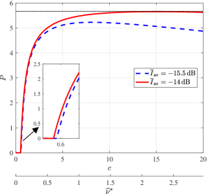
Refer to caption
Figure 4: The optimized P𝑃P obtained from (45a) versus ν^superscript^𝜈\widehat{\nu}^{*} (and c𝑐c) for P¯av=2subscript¯𝑃av2\overline{P}_{\rm{av}}=2\,dB.

To gain an insight on the solution of (P1), we look into the behavior of the optimized P𝑃P versus the realizations of the estimated channel gain ν^superscript^𝜈\widehat{\nu}^{*}. Fig. 4 illustrates the optimized P𝑃P versus ν^superscript^𝜈\widehat{\nu}^{*} (and c𝑐c, where ν^=cmν^superscript^𝜈𝑐subscript𝑚superscript^𝜈\widehat{\nu}^{*}=c\,m_{\widehat{\nu}^{*}} and mν^subscript𝑚superscript^𝜈m_{\widehat{\nu}^{*}} is the mean of ν^superscript^𝜈\widehat{\nu}^{*}) for I¯av=15.5,14subscript¯𝐼av15.514\overline{I}_{\rm{av}}=-15.5,-14\,dB and other simulation parameters given in Table III. For these parameters mν^=0.1484subscript𝑚superscript^𝜈0.1484m_{\widehat{\nu}^{*}}=0.1484. We observe that the optimized P𝑃P for very small ν^superscript^𝜈\widehat{\nu}^{*} (when ν^superscript^𝜈\widehat{\nu}^{*} is smaller than a cut-off threshold ζ=3.5mν^𝜁3.5subscript𝑚superscript^𝜈\zeta=3.5\,m_{\widehat{\nu}^{*}}) is zero. As ν^superscript^𝜈\widehat{\nu}^{*} increases the optimized P𝑃P increases gradually until it reaches a maximum value. As ν^superscript^𝜈\widehat{\nu}^{*} increases further, the optimized P𝑃P decreases, until it reaches a minimum value for very large ν^superscript^𝜈\widehat{\nu}^{*} (when ν^>85mν^superscript^𝜈85subscript𝑚superscript^𝜈\widehat{\nu}^{*}>85\,m_{\widehat{\nu}^{*}}), not shown in the figure. Comparing the curves for I¯av=15.5subscript¯𝐼av15.5\overline{I}_{\rm{av}}=-15.5\,dB and I¯av=14subscript¯𝐼av14\overline{I}_{\rm{av}}=-14\,dB, we note that the optimized P𝑃P decays faster (after it reaches its maximum value) for lower I¯avsubscript¯𝐼av\overline{I}_{\rm{av}}. Moreover, the cut-off threshold ζ𝜁\zeta is lower for higher I¯avsubscript¯𝐼av\overline{I}_{\rm{av}}. The behavior of the optimized P𝑃P versus ν^superscript^𝜈\widehat{\nu}^{*} is different from our intuitive expectation that expects to see the optimized P𝑃P increases monotonically as ν^superscript^𝜈\widehat{\nu}^{*} increases. We explore this by examining the optimized P𝑃P, which satisfies (45a).

Although for general M𝑀M the optimized P𝑃P does not have a closed form expression, for M=1𝑀1M=1 and under a simplifying assumption666We assume that the optimized Ttrsubscript𝑇trT_{\rm{tr}} is large enough such that α~P+σq2σq2~𝛼𝑃superscriptsubscript𝜎q2superscriptsubscript𝜎q2\widetilde{\alpha}P+\sigma_{\rm{q}}^{2}\approx\sigma_{\rm{q}}^{2}. This assumption allows us to approximate (45a) for M=1𝑀1M=1 as a quadratic polynomial in P𝑃P (originally a polynomial of degree 444 in P𝑃P) and find a closed-form expression for P𝑃P. it can approximated as follows:

P[F+Υ2]+,𝑃superscriptdelimited-[]𝐹Υ2\displaystyle\qquad\qquad\quad~{}~{}P\approx\left[\frac{F+\sqrt{\Upsilon}}{2}\right]^{+}, (46)
F𝐹\displaystyle F =β0W(ν^)+β1ln(2)[λ(β0W(ν^)+β1)+μb0]2σq2+σp2ν^,absentsubscript𝛽0𝑊superscript^𝜈subscript𝛽12delimited-[]𝜆subscript𝛽0𝑊superscript^𝜈subscript𝛽1𝜇subscript𝑏02superscriptsubscript𝜎q2superscriptsubscript𝜎p2superscript^𝜈\displaystyle=\frac{\beta_{0}W(\widehat{\nu}^{*})\!+\!\beta_{1}}{\ln(2)\Big{[}\lambda\big{(}\beta_{0}W(\widehat{\nu}^{*})\!+\!\beta_{1}\big{)}\!+\!\mu b_{0}\Big{]}}-\frac{2\sigma_{\rm{q}}^{2}\!+\!\sigma_{\rm{p}}^{2}}{\widehat{\nu}^{*}},
Υ=F2Υsuperscript𝐹2\displaystyle\Upsilon\!=\!F^{2} 4ν^(σq2(σq2+σp2)ν^(β0W(ν^)+β1)σq2+β1σp2ln(2)[λ(β0W(ν^)+β1)+μb0]).4superscript^𝜈superscriptsubscript𝜎q2superscriptsubscript𝜎q2superscriptsubscript𝜎p2superscript^𝜈subscript𝛽0𝑊superscript^𝜈subscript𝛽1superscriptsubscript𝜎q2subscript𝛽1superscriptsubscript𝜎p22delimited-[]𝜆subscript𝛽0𝑊superscript^𝜈subscript𝛽1𝜇subscript𝑏0\displaystyle\!-\!\frac{4}{\widehat{\nu}^{*}}\!\!\left(\!\!\!\frac{\sigma_{\rm{q}}^{2}(\sigma_{\rm{q}}^{2}\!+\!\sigma_{\rm{p}}^{2})}{\widehat{\nu}^{*}}\!-\!\frac{\big{(}\beta_{0}W(\widehat{\nu}^{*})\!+\!\beta_{1}\big{)}\sigma_{\rm{q}}^{2}\!+\!\beta_{1}\sigma_{\rm{p}}^{2}}{\ln(2)\Big{[}\lambda(\beta_{0}W(\widehat{\nu}^{*})\!+\!\beta_{1})\!+\!\mu b_{0}\Big{]}}\!\right)\!.

where W(ν^)=fν^0(ν^)/fν^1(ν^)=α^1/α^0eν^(1α^01α^1)𝑊superscript^𝜈subscriptsuperscript𝑓0superscript^𝜈superscript^𝜈subscriptsuperscript𝑓1superscript^𝜈superscript^𝜈superscript^𝛼1superscript^𝛼0superscript𝑒superscript^𝜈1superscript^𝛼01superscript^𝛼1W(\widehat{\nu}^{*})=f^{0}_{\widehat{\nu}^{*}}(\widehat{\nu}^{*})/f^{1}_{\widehat{\nu}^{*}}(\widehat{\nu}^{*})=\widehat{\alpha}^{1}/\widehat{\alpha}^{0}~{}e^{-\widehat{\nu}^{*}(\frac{1}{\widehat{\alpha}^{0}}-\frac{1}{\widehat{\alpha}^{1}})}. Considering (21) we realize that α^0<α^1superscript^𝛼0superscript^𝛼1\widehat{\alpha}^{0}<\widehat{\alpha}^{1}. This implies as ν^superscript^𝜈\widehat{\nu}^{*} increases, W(ν^)𝑊superscript^𝜈W(\widehat{\nu}^{*}) and ΥΥ\Upsilon decrease. However, the behavior of F𝐹F changes, i.e., F𝐹F increases until it reaches a maximum value. As ν^superscript^𝜈\widehat{\nu}^{*} increases further, F𝐹F decreases. Considering (46) we note that the behavior of P𝑃P (in terms of ν^superscript^𝜈\widehat{\nu}^{*}) is dominated by the behavior of F𝐹F. In the ideal scenario when there is no channel estimation error, we have α^0=α^1=αsuperscript^𝛼0superscript^𝛼1𝛼\widehat{\alpha}^{0}=\widehat{\alpha}^{1}=\alpha and W(ν^)=1𝑊superscript^𝜈1W(\widehat{\nu}^{*})=1, F𝐹F monotonically increases and ΥΥ\Upsilon deceases, i.e., P𝑃P in (46) monotonically increases as ν^superscript^𝜈\widehat{\nu}^{*} increases, which is what we intuitively expect.

TABLE II: Pr(ν^cmν^)Prsuperscript^𝜈𝑐subscript𝑚superscript^𝜈\Pr(\widehat{\nu}^{*}\geq c\,m_{\widehat{\nu}^{*}}) in terms of c𝑐c, given mν^=0.1484subscript𝑚superscript^𝜈0.1484m_{\widehat{\nu}^{*}}=0.1484.
c𝑐c Pr(ν^cmν^)Prsuperscript^𝜈𝑐subscript𝑚superscript^𝜈\Pr(\widehat{\nu}^{*}\geq c\,m_{\widehat{\nu}^{*}})
444 3.01×1033.01superscript1033.01\times 10^{-3}
888 7.04×1067.04superscript1067.04\times 10^{-6}
121212 1.54×1081.54superscript1081.54\times 10^{-8}
161616 4.87×10114.87superscript10114.87\times 10^{-11}

The optimized P𝑃P we discussed so far requires solving (45) several times for each realization of ν^superscript^𝜈\widehat{\nu}^{*}. Integrating the insights we have gained into how this optimized P𝑃P varies in terms of ν^superscript^𝜈\widehat{\nu}^{*}, we propose two transmit power control schemes that are simpler to implement and yield achievable rate lower bounds that are very close to the maximized RLBsubscript𝑅LBR_{\rm{LB}} values in (P1). Since Pr(ν^cmν^)Prsuperscript^𝜈𝑐subscript𝑚superscript^𝜈\Pr(\widehat{\nu}^{*}\geq c\,m_{\widehat{\nu}^{*}}) is very small for c8𝑐8c\geq 8 (see Table II), we focus on the regime when ν^<8mν^superscript^𝜈8subscript𝑚superscript^𝜈\widehat{\nu}^{*}<8\,m_{\widehat{\nu}^{*}} and develop two schemes, dubbed here scheme 1 and scheme 2, that mimic the behavior of the optimized P𝑃P in this regime.

VI-A Scheme 1

For scheme 1, when the spectrum is sensed idle, SUtx sends data to SUrx over the selected sector i=mSR𝑖superscriptsubscript𝑚SRi=m_{\rm{SR}}^{*} according to the following rule:

PS1={Π1,ifν^ζ10,ifν^<ζ1subscript𝑃subscriptS1casessubscriptΠ1ifsuperscript^𝜈subscript𝜁10ifsuperscript^𝜈subscript𝜁1P_{\rm{S}_{1}}=\left\{\begin{array}[]{ll}{\Pi}_{1},&\text{if}~{}~{}\widehat{\nu}^{*}\geq\zeta_{1}\\ 0,&\text{if}~{}~{}\widehat{\nu}^{*}<\zeta_{1}\\ \end{array}\right. (47)

i.e., when ν^superscript^𝜈\widehat{\nu}^{*} is less than a cut-off threshold ζ1subscript𝜁1\zeta_{1}, SUtx remains silent, when ν^superscript^𝜈\widehat{\nu}^{*} is larger than ζ1subscript𝜁1\zeta_{1}, SUtx lets its transmit power be equal to constant Π1subscriptΠ1\Pi_{1}. The parameter Π1subscriptΠ1\Pi_{1} can be found in terms of Tse,Ttr,ζ1subscript𝑇sesubscript𝑇trsubscript𝜁1T_{\rm{se}},T_{\rm{tr}},\zeta_{1}, via enforcing AIC in (41) and ATPC in (43) as the following:

Π1=1Ddmin{P¯avπ^0DtrPtr=01β(1Fν^(ζ1)),I¯avu0DtrPtrb0(1Fν^1(ζ1))}.subscriptΠ11subscript𝐷dsubscript¯𝑃avsubscript^𝜋0subscript𝐷trsubscript𝑃trsuperscriptsubscript01subscript𝛽1subscriptsuperscript𝐹superscript^𝜈subscript𝜁1subscript¯𝐼avsubscript𝑢0subscript𝐷trsubscript𝑃trsubscript𝑏01subscriptsuperscript𝐹1superscript^𝜈subscript𝜁1\Pi_{1}={1\over D_{\rm{d}}}\min\!\left\{\frac{\overline{P}_{\rm{av}}-{\widehat{\pi}_{0}D_{\rm{tr}}P_{\rm{tr}}}}{\sum_{\ell=0}^{1}\beta_{\ell}\big{(}1\!-\!F^{\ell}_{\widehat{\nu}^{*}}(\zeta_{1})\big{)}}\,,\,\frac{\overline{I}_{\rm{av}}{-u_{0}D_{\rm{tr}}P_{\rm{tr}}}}{b_{0}\big{(}1\!-\!F^{1}_{\widehat{\nu}^{*}}(\zeta_{1})\big{)}}\right\}\!. (48)

Let RS1subscript𝑅subscriptS1R_{\rm{S}_{1}} denote the lower bound on the achievable rates when SUtx adopts the power control scheme in (47). We find RS1subscript𝑅subscriptS1R_{\rm{S}_{1}} expression by substituting PS1subscript𝑃subscriptS1P_{\rm{S}_{1}} in (V) and taking expectation w.r.t. ν^superscript^𝜈\widehat{\nu}^{*}. This expression is given in (49) where SNRi0=Π1α^i0+σq2subscriptsuperscriptSNR0𝑖subscriptΠ1subscriptsuperscript^𝛼0𝑖superscriptsubscript𝜎q2\text{SNR}^{0}_{i}={\Pi_{1}\over\widehat{\alpha}^{0}_{i}+\sigma_{\rm{q}}^{2}}, SNRi1=Π1α^i1+σq2+σp2subscriptsuperscriptSNR1𝑖subscriptΠ1subscriptsuperscript^𝛼1𝑖superscriptsubscript𝜎q2superscriptsubscript𝜎p2\text{SNR}^{1}_{i}={\Pi_{1}\over\widehat{\alpha}^{1}_{i}+\sigma_{\rm{q}}^{2}+\sigma_{\rm{p}}^{2}} and Ei()Ei\text{Ei}(\cdot) is the exponential integral.

RS1=Ddln(2)=01βj=1M[Y(α^j,SNRj)+m=1mjM(1)mmY(dj,m,SNRj)]subscript𝑅subscriptS1subscript𝐷d2superscriptsubscript01subscript𝛽superscriptsubscript𝑗1𝑀delimited-[]𝑌subscriptsuperscript^𝛼𝑗superscriptsubscriptSNR𝑗superscriptsubscript𝑚𝑗𝑚1𝑀superscript1𝑚subscript𝑚𝑌subscriptsuperscript𝑑𝑗𝑚superscriptsubscriptSNR𝑗R_{\rm{S}_{1}}=\,{D_{\rm{d}}\over\ln(2)}\sum_{\ell=0}^{1}\beta_{\ell}\sum_{j=1}^{M}\bigg{[}Y\big{(}\widehat{\alpha}^{\ell}_{j},\text{SNR}_{j}^{\ell}\big{)}+\sum_{\underset{m\neq j}{m=1}}^{M}(-1)^{m}\sum\nolimits_{m}Y\big{(}d^{\ell}_{j,m},\text{SNR}_{j}^{\ell}\big{)}\bigg{]} (49)
Y(a,b)=ζ1ln(1+bx)1aexa𝑑x=eζ1/aln(1+bζ1)e1/abEi(ζ1/a1/ab),dj,m=(Ak1:km+1α~j)1.formulae-sequence𝑌𝑎𝑏superscriptsubscriptsubscript𝜁11𝑏𝑥1𝑎superscript𝑒𝑥𝑎differential-d𝑥superscript𝑒subscript𝜁1𝑎1𝑏subscript𝜁1superscript𝑒1𝑎𝑏Eisubscript𝜁1𝑎1𝑎𝑏subscriptsuperscript𝑑𝑗𝑚superscriptsubscriptsuperscript𝐴:subscript𝑘1subscript𝑘𝑚1superscriptsubscript~𝛼𝑗1Y(a,b)\!=\!\int_{\zeta_{1}}^{\infty}\!\!\ln(1+bx){1\over a}e^{-x\over a}dx=e^{-\zeta_{1}/a}\ln\big{(}1+b\zeta_{1}\big{)}-e^{1/ab}~{}\text{Ei}\big{(}-\zeta_{1}/a-1/ab\big{)},\qquad~{}~{}d^{\ell}_{j,m}\!=\!\left(A^{\ell}_{k_{1}:k_{m}}+{1\over\widetilde{\alpha}_{j}^{\ell}}\right)^{-1}.

With this transmit power scheme, we consider a modified problem to (P1), where the lower bound RS1subscript𝑅subscriptS1R_{\rm{S}_{1}} in (49) is maximized (subject to the same constraints) and the optimization variables are Tse,Ttr,ζ1subscript𝑇sesubscript𝑇trsubscript𝜁1T_{\rm{se}},T_{\rm{tr}},\zeta_{1}. In Section VII we numerically compare the maximized RLBsubscript𝑅LBR_{\rm{LB}} in (P1) and the maximized RS1subscript𝑅subscriptS1R_{\rm{S}_{1}}.

VI-B Scheme 2

For scheme 2, when the spectrum is sensed idle, SUtx sends data symbols to SUrx over the selected sector i=mSR𝑖superscriptsubscript𝑚SRi=m_{\rm{SR}}^{*} according to the following rule:

PS2={Π2(1ζ2ν^),ifν^ζ20,ifν^<ζ2subscript𝑃subscriptS2casessubscriptΠ21subscript𝜁2superscript^𝜈ifsuperscript^𝜈subscript𝜁20ifsuperscript^𝜈subscript𝜁2P_{\rm{S}_{2}}=\left\{\begin{array}[]{ll}\Pi_{2}\big{(}1-\frac{\zeta_{2}}{\widehat{\nu}^{*}}\big{)},&\text{if}~{}~{}\widehat{\nu}^{*}\geq\zeta_{2}\\ 0,&\text{if}~{}~{}\widehat{\nu}^{*}<\zeta_{2}\\ \end{array}\right. (50)

Different from scheme 1, in the scheme 2 when ν^superscript^𝜈\widehat{\nu}^{*} exceeds the cut-off threshold ζ2subscript𝜁2\zeta_{2}, SUtx transmits at a variable power. The power level increases as ν^superscript^𝜈\widehat{\nu}^{*} increases, until it reaches its maximum value of Π2subscriptΠ2\Pi_{2}, i.e., limν^PS2=Π2subscriptsuperscript^𝜈subscript𝑃subscriptS2subscriptΠ2\lim_{\widehat{\nu}^{*}\to\infty}P_{\rm{S}_{2}}=\Pi_{2}. The parameter Π2subscriptΠ2\Pi_{2} can be found in terms of Tse,Ttr,ζ2subscript𝑇sesubscript𝑇trsubscript𝜁2T_{\rm{se}},T_{\rm{tr}},\zeta_{2}, via enforcing AIC in (41) and ATPC in (43) as the following:

Π2=1Ddmin{P¯avπ^0DtrPtr=01β[1G(ζ2)],I¯avu0DtrPtrb0[1G1(ζ2)]},subscriptΠ21subscript𝐷dsubscript¯𝑃avsubscript^𝜋0subscript𝐷trsubscript𝑃trsuperscriptsubscript01subscript𝛽delimited-[]1superscript𝐺subscript𝜁2subscript¯𝐼avsubscript𝑢0subscript𝐷trsubscript𝑃trsubscript𝑏0delimited-[]1superscript𝐺1subscript𝜁2\Pi_{2}={1\over D_{\rm{d}}}\min\!\left\{\frac{\overline{P}_{\rm{av}}-{\widehat{\pi}_{0}D_{\rm{tr}}P_{\rm{tr}}}}{\sum\nolimits_{\ell=0}^{1}\beta_{\ell}\big{[}1\!-\!G^{\ell}(\zeta_{2})\big{]}}\,,\,\frac{\overline{I}_{\rm{av}}{-u_{0}D_{\rm{tr}}P_{\rm{tr}}}}{b_{0}\big{[}1\!-\!G^{1}(\zeta_{2})\big{]}}\right\}, (51)

where G(ζ2)=Fν^(ζ2)+ζ2T(ζ2)superscript𝐺subscript𝜁2subscriptsuperscript𝐹superscript^𝜈subscript𝜁2subscript𝜁2superscript𝑇subscript𝜁2G^{\ell}(\zeta_{2})=F^{\ell}_{\widehat{\nu}^{*}}(\zeta_{2})+\zeta_{2}T^{\ell}(\zeta_{2}) and

T(ζ2)=superscript𝑇subscript𝜁2absent\displaystyle T^{\ell}(\zeta_{2})= 𝔼{1ν^|ν^ζ2,}=ζ2fν^(y)y𝑑y𝔼conditional-set1superscript^𝜈superscript^𝜈subscript𝜁2subscriptsuperscriptsubscriptsubscript𝜁2subscriptsuperscript𝑓superscript^𝜈𝑦𝑦differential-d𝑦\displaystyle\,\mathbb{E}\left\{{1\over\widehat{\nu}^{*}}\,\big{|}\,\widehat{\nu}^{*}\geq\zeta_{2},\,{\cal H}_{\ell}\right\}=\int_{\zeta_{2}}^{\infty}{f^{\ell}_{\widehat{\nu}^{*}}(y)\over y}dy
=\displaystyle= m=1M(1)mmAj1:jmEi(ζ2Aj1:jm).superscriptsubscript𝑚1𝑀superscript1𝑚subscript𝑚subscriptsuperscript𝐴:subscript𝑗1subscript𝑗𝑚Eisubscript𝜁2subscriptsuperscript𝐴:subscript𝑗1subscript𝑗𝑚\displaystyle\,\sum_{m=1}^{M}\!(-1)^{m}\sum\nolimits_{m}A^{\ell}_{j_{1}:j_{m}}\text{Ei}\big{(}\!-\!\zeta_{2}A^{\ell}_{j_{1}:j_{m}}\big{)}. (52)

Let RS2subscript𝑅subscriptS2R_{\rm{S}_{2}} represent the lower bound on the achievable rates when SUtx adopts the power control scheme in (50). We find RS2subscript𝑅subscriptS2R_{\rm{S}_{2}} by substituting PS2subscript𝑃subscriptS2P_{\rm{S}_{2}} in (V) and taking expectation w.r.t. ν^superscript^𝜈\widehat{\nu}^{*}. With this transmit power scheme, we consider a modified problem to (P1), where the lower bound RS2subscript𝑅subscriptS2R_{\rm{S}_{2}} is maximized (subject to the same constraints) and the optimization variables are Tse,Ttr,ζ2subscript𝑇sesubscript𝑇trsubscript𝜁2T_{\rm{se}},T_{\rm{tr}},\zeta_{2}. In Section VII we numerically compare the maximized RLBsubscript𝑅LBR_{\rm{LB}} in (P1) and the maximized RS2subscript𝑅subscriptS2R_{\rm{S}_{2}}. Note that the closed-form expression for RS2subscript𝑅subscriptS2R_{\rm{S}_{2}} cannot be obtained.

VII Simulation Results

TABLE III: Simulation Parameters
Parameter Value Parameter Value Parameter Value
A0subscript𝐴0A_{0} 0.980.980.98 γsssubscript𝛾ss\gamma_{\rm{ss}} 0.10.10.1 σw2,σq2superscriptsubscript𝜎w2superscriptsubscript𝜎q2\sigma_{\rm{w}}^{2},\sigma_{\rm{q}}^{2} 0.50.50.5
A1subscript𝐴1A_{1} 0.020.020.02 γ,γsp𝛾subscript𝛾sp\gamma,\gamma_{\rm{sp}} 0.50.50.5 Ppsubscript𝑃pP_{\rm{p}} 0.50.50.5 watts
ϕ3dBsubscriptitalic-ϕ3dB\phi_{\rm{3dB}} 20°superscript20°20^{\degree} π1subscript𝜋1\pi_{1} 0.70.70.7 Tfsubscript𝑇fT_{\rm{f}} 303030 ms
ϕ1subscriptitalic-ϕ1\phi_{1} 55°superscript55°-55^{\degree} P¯dsubscript¯𝑃d{\overline{P}}_{\rm{d}} 0.850.850.85 Ptrsubscript𝑃trP_{\rm{tr}} 222 watts
ϕ2subscriptitalic-ϕ2\phi_{2} +55°superscript55°+55^{\degree} M𝑀M 777

We corroborate our analysis on constrained maximization of achievable rate lower bounds with Matlab simulations. Our simulation parameters are given in Table III. We start by illustrating the the behavior of our proposed power allocation schemes versus ν^superscript^𝜈\widehat{\nu}^{*}. Fig. 5 shows the optimized P𝑃P obtained by solving (45a) and the two proposed suboptimal schemes PS2subscript𝑃subscriptS2P_{\rm{S}_{2}} and PS1subscript𝑃subscriptS1P_{\rm{S}_{1}} versus ν^superscript^𝜈\widehat{\nu}^{*}. We observe that PS2subscript𝑃subscriptS2P_{\rm{S}_{2}} and PS1subscript𝑃subscriptS1P_{\rm{S}_{1}} mimic the behavior of the optimized P𝑃P. Furthermore, for the cut-off thresholds we have ζ<ζ1<ζ2𝜁subscript𝜁1subscript𝜁2\zeta<\zeta_{1}<\zeta_{2}.

Next, we explore the effect of spatial spectrum sensing duration Tsesubscript𝑇seT_{\rm{se}} on the achievable rate lower bounds of our system. Fig. 6 shows the maximized RLB,RS2subscript𝑅LBsubscript𝑅subscriptS2R_{\rm{LB}},R_{\rm{S}_{2}} and RS1subscript𝑅subscriptS1R_{\rm{S}_{1}} (which we refer in the figures to as “Rate”) versus Tsesubscript𝑇seT_{\rm{se}}. To plot this figure, we maximize the bounds w.r.t. only Ttrsubscript𝑇trT_{\rm{tr}} and P𝑃P, subject to ATPC and AIC. We note that for all Tsesubscript𝑇seT_{\rm{se}} values we have RLB>RS2>RS1subscript𝑅LBsubscript𝑅subscriptS2subscript𝑅subscriptS1R_{\rm{LB}}>R_{\rm{S}_{2}}>R_{\rm{S}_{1}}. We observe that the achievable rates always have a maximum in the interval (0,TfTtr)0subscript𝑇fsubscript𝑇tr(0,T_{\rm{f}}-T_{\rm{tr}}). For the simulation parameters in Table III the optimized Tse=0.75ms=2.5%Tfsubscript𝑇se0.75mspercent2.5subscript𝑇fT_{\rm{se}}=0.75\,\text{ms}=2.5\%\,T_{\rm{f}}. Also, scheme 2 yields a higher achievable rate than that of scheme 1, because its corresponding power PS2subscript𝑃subscriptS2P_{\rm{S}_{2}} fits better to the optimized power P𝑃P obtained from solving (45a). The achievable rate RS2subscript𝑅subscriptS2R_{\rm{S}_{2}} is very close to RLBsubscript𝑅LBR_{\rm{LB}} and we do not have a significant performance loss if we choose the simple transmit power control scheme in (50).
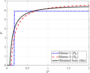
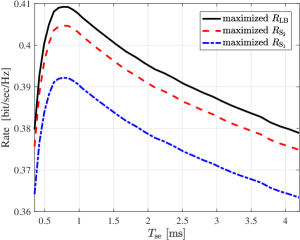
Refer to caption
Figure 5: P𝑃P versus ν^superscript^𝜈\widehat{\nu}^{*} for P¯av=2dB,I¯av=12formulae-sequencesubscript¯𝑃av2dBsubscript¯𝐼av12\overline{P}_{\rm{av}}=2\,\text{dB},\overline{I}_{\rm{av}}=-12\,dB .
Refer to caption
Figure 6: Rate versus Tsesubscript𝑇seT_{\rm{se}} for P¯av=2dB,I¯av=15formulae-sequencesubscript¯𝑃av2dBsubscript¯𝐼av15\overline{P}_{\rm{av}}=2\,\text{dB},\overline{I}_{\rm{av}}=-15\,dB.

To investigate the effect of channel training duration Ttrsubscript𝑇trT_{\rm{tr}} on the achievable rate lower bounds, we plot Fig. 7 which illustrates the maximized RLB,RS2subscript𝑅LBsubscript𝑅subscriptS2R_{\rm{LB}},R_{\rm{S}_{2}} and RS1subscript𝑅subscriptS1R_{\rm{S}_{1}} versus Ttrsubscript𝑇trT_{\rm{tr}}. To plot this figure, we maximize the bounds w.r.t. only Tsesubscript𝑇seT_{\rm{se}} and P𝑃P, subject to ATPC and AIC. For all Ttrsubscript𝑇trT_{\rm{tr}} values we have RLB>RS2>RS1subscript𝑅LBsubscript𝑅subscriptS2subscript𝑅subscriptS1R_{\rm{LB}}>R_{\rm{S}_{2}}>R_{\rm{S}_{1}}. We observe that the achievable rates always have a maximum in the interval (0,TfTse)0subscript𝑇fsubscript𝑇se(0,T_{\rm{f}}-T_{\rm{se}}). For the simulation parameters in Table III the optimized Ttr=0.67ms=2.23%Tfsubscript𝑇tr0.67mspercent2.23subscript𝑇fT_{\rm{tr}}=0.67\,\text{ms}=2.23\%\,T_{\rm{f}}. Comparing Fig. 7 and Fig. 6, we notice that the achievable rates are more sensitive to the variations of Ttrsubscript𝑇trT_{\rm{tr}} compared to that of Tsesubscript𝑇seT_{\rm{se}}.

Refer to caption
Figure 7: Rate versus Ttrsubscript𝑇trT_{\rm{tr}} for P¯av=2dB,I¯av=15formulae-sequencesubscript¯𝑃av2dBsubscript¯𝐼av15\overline{P}_{\rm{av}}=2\,\text{dB},\overline{I}_{\rm{av}}=-15\,dB.

To be more specific, considering Fig. 6 and Fig. 7, suppose we choose Tsesubscript𝑇seT_{\rm{se}} and Ttrsubscript𝑇trT_{\rm{tr}} values that are different from their corresponding maximum values by 20%percent2020\%, i.e., ΔTse=20%,ΔTtr=20%formulae-sequenceΔsubscript𝑇sepercent20Δsubscript𝑇trpercent20\Delta T_{\rm{se}}=20\%,\Delta T_{\rm{tr}}=20\%. Then

ΔRLB/ΔTtr>ΔRLB/ΔTse,Δsubscript𝑅LBΔsubscript𝑇trΔsubscript𝑅LBΔsubscript𝑇se\displaystyle\Delta R_{\rm{LB}}/\Delta T_{\rm{tr}}>\Delta R_{\rm{LB}}/\Delta T_{\rm{se}},
ΔRS2/ΔTtr>ΔRS2/ΔTse,Δsubscript𝑅subscriptS2Δsubscript𝑇trΔsubscript𝑅subscriptS2Δsubscript𝑇se\displaystyle\Delta R_{\rm{S}_{2}}/\Delta T_{\rm{tr}}>\Delta R_{\rm{S}_{2}}/\Delta T_{\rm{se}},
ΔRS1/ΔTtr>ΔRS1/ΔTse.Δsubscript𝑅subscriptS1Δsubscript𝑇trΔsubscript𝑅subscriptS1Δsubscript𝑇se\displaystyle\Delta R_{\rm{S}_{1}}/\Delta T_{\rm{tr}}>\Delta R_{\rm{S}_{1}}/\Delta T_{\rm{se}}.

These indicate that proper allocation of Ttrsubscript𝑇trT_{\rm{tr}} is more important than that of Tsesubscript𝑇seT_{\rm{se}}, for providing higher achievable rates in our system.

To explore the effects of the number of beams M𝑀M and I¯avsubscript¯𝐼av\overline{I}_{\rm{av}} on the achievable rate lower bounds, Fig. 8 illustrates the maximized RLB,RS2,RS1subscript𝑅LBsubscript𝑅subscriptS2subscript𝑅subscriptS1R_{\rm{LB}},R_{\rm{S}_{2}},R_{\rm{S}_{1}} versus I¯avsubscript¯𝐼av\overline{I}_{\rm{av}} for M=7,11𝑀711M=7,11 and P¯av=2subscript¯𝑃av2\overline{P}_{\rm{av}}=2 dB. We observe that as M𝑀M increases a higher rate can be achieved. For all M𝑀M and I¯avsubscript¯𝐼av\overline{I}_{\rm{av}} values we have RLB>RS2>RS1subscript𝑅LBsubscript𝑅subscriptS2subscript𝑅subscriptS1R_{\rm{LB}}>R_{\rm{S}_{2}}>R_{\rm{S}_{1}}. We realize that as I¯avsubscript¯𝐼av\overline{I}_{\rm{av}} increases from 1818-18\,dB to 1414-14\,dB, the achievable rates are monotonically increasing and the AIC is dominant. However, as I¯avsubscript¯𝐼av\overline{I}_{\rm{av}} increases beyond 1414-14\,dB, the achievable rates remain unchanged and the ATPC is dominant.
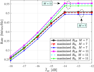
Refer to caption
Figure 8: Rate versus I¯avsubscript¯𝐼av\overline{I}_{\rm{av}} for M=7,11𝑀711M=7,11 and P¯av=2subscript¯𝑃av2\overline{P}_{\rm{av}}=2 dB.

Fig. 9 illustrates the maximized RLB,RS2,RS1subscript𝑅LBsubscript𝑅subscriptS2subscript𝑅subscriptS1R_{\rm{LB}},R_{\rm{S}_{2}},R_{\rm{S}_{1}} versus P¯avsubscript¯𝑃av\overline{P}_{\rm{av}} for M=7,11𝑀711M=7,11 and I¯av=14subscript¯𝐼av14\overline{I}_{\rm{av}}=-14 dB. The behaviors of the achievable rates in terms of M𝑀M are the same as Fig. 8. We note that as P¯avsubscript¯𝑃av\overline{P}_{\rm{av}} increases from 44-4\,dB to 222\,dB, the achievable rates are monotonically increasing and the ATPC is dominant. However, as P¯avsubscript¯𝑃av\overline{P}_{\rm{av}} increases beyond 222\,dB, the achievable rates remain unchanged and the AIC is dominant.
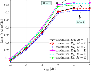
Refer to caption
Figure 9: Rate versus P¯avsubscript¯𝑃av\overline{P}_{\rm{av}} for M=7,11𝑀711M=7,11 and I¯av=14subscript¯𝐼av14\overline{I}_{\rm{av}}=-14 dB.

We also consider outage probability as another performance metric to evaluate our system. We define the outage probability as the probability of SUtx not transmitting data symbols due to the weak SUtx-SUrx channel when the spectrum is sensed idle, i.e., Pout=Pr{P=0|^0}subscript𝑃outPr𝑃conditional0subscript^0P_{\rm{out}}=\Pr\big{\{}P=0\,|\,\widehat{\cal H}_{0}\big{\}}. This probability can be directly obtained using the CDF of ν^superscript^𝜈\widehat{\nu}^{*} evaluated at the cut-off threshold as the following

Pout=subscript𝑃outabsent\displaystyle P_{\rm{out}}= Pr(ν^ζ|^0)=ω0Fν^0(ζ)+ω1Fν^1(ζ),Prsuperscript^𝜈conditional𝜁subscript^0subscript𝜔0subscriptsuperscript𝐹0superscript^𝜈𝜁subscript𝜔1subscriptsuperscript𝐹1superscript^𝜈𝜁\displaystyle\Pr(\widehat{\nu}^{*}\leq\zeta|\widehat{\cal H}_{0})=\omega_{0}F^{0}_{\widehat{\nu}^{*}}(\zeta)~{}+\omega_{1}F^{1}_{\widehat{\nu}^{*}}(\zeta),
Pout,S1=subscript𝑃outsubscriptS1absent\displaystyle P_{\rm{out},\rm{S}_{1}}= Pr(ν^ζ1|^0)=ω0Fν^0(ζ1)+ω1Fν^1(ζ1),Prsuperscript^𝜈conditionalsubscript𝜁1subscript^0subscript𝜔0subscriptsuperscript𝐹0superscript^𝜈subscript𝜁1subscript𝜔1subscriptsuperscript𝐹1superscript^𝜈subscript𝜁1\displaystyle\Pr(\widehat{\nu}^{*}\leq\zeta_{1}|\widehat{\cal H}_{0})=\omega_{0}F^{0}_{\widehat{\nu}^{*}}(\zeta_{1})+\omega_{1}F^{1}_{\widehat{\nu}^{*}}(\zeta_{1}),
Pout,S2=subscript𝑃outsubscriptS2absent\displaystyle P_{\rm{out},\rm{S}_{2}}= Pr(ν^ζ2|^0)=ω0Fν^0(ζ2)+ω1Fν^1(ζ2).Prsuperscript^𝜈conditionalsubscript𝜁2subscript^0subscript𝜔0subscriptsuperscript𝐹0superscript^𝜈subscript𝜁2subscript𝜔1subscriptsuperscript𝐹1superscript^𝜈subscript𝜁2\displaystyle\Pr(\widehat{\nu}^{*}\leq\zeta_{2}|\widehat{\cal H}_{0})=\omega_{0}F^{0}_{\widehat{\nu}^{*}}(\zeta_{2})+\omega_{1}F^{1}_{\widehat{\nu}^{*}}(\zeta_{2}).

Fig. 10 illustrates Pout,Pout,S2,Pout,S1subscript𝑃outsubscript𝑃outsubscriptS2subscript𝑃outsubscriptS1P_{\rm{out}},P_{\rm{out},\rm{S}_{2}},P_{\rm{out},\rm{S}_{1}} versus P¯avsubscript¯𝑃av\overline{P}_{\rm{av}} for I¯av=8subscript¯𝐼av8\overline{I}_{\rm{av}}=-8\,dB. We observe that as P¯avsubscript¯𝑃av\overline{P}_{\rm{av}} increases the outage probabilities decrease. Moreover, for a given P¯avsubscript¯𝑃av\overline{P}_{\rm{av}} we have Pout<Pout,S2<Pout,S1subscript𝑃outsubscript𝑃outsubscriptS2subscript𝑃outsubscriptS1P_{\rm{out}}<P_{\rm{out},\rm{S}_{2}}<P_{\rm{out},\rm{S}_{1}}. This is consistent with Fig. 5 which shows for a given P¯avsubscript¯𝑃av\overline{P}_{\rm{av}}, we have ζ<ζ1<ζ2𝜁subscript𝜁1subscript𝜁2\zeta<\zeta_{1}<\zeta_{2}. Combined this with the fact that the CFD Fν^()subscript𝐹superscript^𝜈F_{\widehat{\nu}^{*}}(\cdot) is an increasing function of its argument, we reach the conclusion that Pout<Pout,S2<Pout,S1subscript𝑃outsubscript𝑃outsubscriptS2subscript𝑃outsubscriptS1P_{\rm{out}}<P_{\rm{out},\rm{S}_{2}}<P_{\rm{out},\rm{S}_{1}}.

Refer to caption
Figure 10: Poutsubscript𝑃outP_{\rm{out}} versus P¯avsubscript¯𝑃av\overline{P}_{\rm{av}} for I¯av=8subscript¯𝐼av8\overline{I}_{\rm{av}}=-8\,dB.

VIII Conclusions

We considered an opportunistic CR system consisting of a PU, SUtx, and SUrx, where SUtx is equipped with a RA that has M𝑀M beams, and there is an error-free low-rate feedback channel from SUrx to SUtx. We proposed a system design for integrated sector-based spatial spectrum sensing and sector-based data symbol communication. We studied the entangled effects of spectrum sensing error, channel estimation error, and beam detection and beam selection errors (introduced by the RA), on the system achievable rates. We formulated a constrained optimization problem, where a lower bound on the achievable rate of SUtx–SUrx link is maximized, subject to ATPC and AIC, with the optimization variables being the durations of spatial spectrum sensing Tsesubscript𝑇seT_{\rm{se}} and channel training Ttrsubscript𝑇trT_{\rm{tr}} as well as data symbol transmission power at SUtx. Moreover, we proposed two alternative power adaptation schemes that are simpler to implement. We solved the proposed constrained optimization problems using iterative methods based on the BCD algorithm. Our simulation results demonstrate that one can increase the achievable rates of SUtx–SUrx link significantly, via implementing these optimizations, while maintaining the ATPC and AIC. They also showed that the achievable rates obtained from employing simple schemes 1 and 2 are very close to the one produced by the optimized transmit power. Our numerical results also showed that between optimizing Tsesubscript𝑇seT_{\rm{se}} and Ttrsubscript𝑇trT_{\rm{tr}}, optimizing the latter has a larger effect on increasing the achievable rates in our system.

Acknowledgment

This research was supported by NSF under grant ECCS-1443942.

References

  • [1] A. Goldsmith, S. A. Jafar, I. Maric, and S. Srinivasa, “Breaking spectrum gridlock with cognitive radios: An information theoretic perspective,” Proceedings of the IEEE, vol. 97, no. 5, pp. 894–914, May 2009.
  • [2] H. Yazdani and A. Vosoughi, “On cognitive radio systems with directional antennas and imperfect spectrum sensing,” in 2017 IEEE International Conference on Acoustics, Speech and Signal Processing (ICASSP), March 2017, pp. 3589–3593.
  • [3] M. Joneidi, H. Yazdani, A. Vosoughi, and N. Rahnavard, “Source localization and tracking for dynamic radio cartography using directional antennas,” in 2019 16th Annual IEEE International Conference on Sensing, Communication, and Networking (SECON), 2019, pp. 1–9.
  • [4] Z. Rezki and M. Alouini, “Ergodic capacity of cognitive radio under imperfect channel-state information,” IEEE Transactions on Vehicular Technology, vol. 61, no. 5, pp. 2108–2119, Jun 2012.
  • [5] D. Xu, Z. Feng, and P. Zhang, “On the impacts of channel estimation errors and feedback delay on the ergodic capacity for spectrum sharing cognitive radio,” Wireless Personal Communications, vol. 72, no. 4, pp. 1875–1887, Oct 2013.
  • [6] H. A. Suraweera, P. J. Smith, and M. Shafi, “Capacity limits and performance analysis of cognitive radio with imperfect channel knowledge,” IEEE Transactions on Vehicular Technology, vol. 59, no. 4, pp. 1811–1822, May 2010.
  • [7] L. Sboui, Z. Rezki, and M. Alouini, “A unified framework for the ergodic capacity of spectrum sharing cognitive radio systems,” IEEE Transactions on Wireless Communications, vol. 12, no. 2, pp. 877–887, February 2013.
  • [8] P. J. Smith, P. A. Dmochowski, H. A. Suraweera, and M. Shafi, “The effects of limited channel knowledge on cognitive radio system capacity,” IEEE Transactions on Vehicular Technology, vol. 62, no. 2, pp. 927–933, Feb 2013.
  • [9] A. Kaushik, S. K. Sharma, S. Chatzinotas, B. Ottersten, and F. K. Jondral, “On the performance analysis of underlay cognitive radio systems: A deployment perspective,” IEEE Transactions on Cognitive Communications and Networking, vol. 2, no. 3, pp. 273–287, Sep. 2016.
  • [10] S. Kashyap and N. B. Mehta, “Optimal binary power control for underlay CR with different interference constraints and impact of channel estimation errors,” IEEE Transactions on Communications, vol. 62, no. 11, pp. 3753–3764, Nov 2014.
  • [11] H. Yazdani and A. Vosoughi, “On the combined effect of directional antennas and imperfect spectrum sensing upon ergodic capacity of cognitive radio systems,” in 2017 51st Asilomar Conference on Signals, Systems, and Computers, Oct 2017, pp. 1702–1706.
  • [12] H. Yazdani and A. Vosoughi, “On optimal sensing and capacity trade-off in cognitive radio systems with directional antennas,” in 2018 IEEE Global Conference on Signal and Information Processing (GlobalSIP), Nov 2018, pp. 1015–1019.
  • [13] A. Kaushik, S. K. Sharma, S. Chatzinotas, B. Ottersten, and F. K. Jondral, “Sensing-throughput tradeoff for interweave cognitive radio system: A deployment-centric viewpoint,” IEEE Transactions on Wireless Communications, vol. 15, no. 5, pp. 3690–3702, May 2016.
  • [14] S. Akin and M. C. Gursoy, “Performance analysis of cognitive radio systems under QoS constraints and channel uncertainty,” IEEE Transactions on Wireless Communications, vol. 10, no. 9, pp. 2883–2895, September 2011.
  • [15] S. Akin and M. C. Gursoy, “Performance analysis of cognitive radio systems with imperfect channel sensing and estimation,” IEEE Transactions on Communications, vol. 63, no. 5, pp. 1554–1566, May 2015.
  • [16] G. Ozcan, M. C. Gursoy, N. Tran, and J. Tang, “Energy-efficient power allocation in cognitive radio systems with imperfect spectrum sensing,” IEEE Journal on Selected Areas in Communications, vol. 34, no. 12, pp. 3466–3481, Dec 2016.
  • [17] L. Zhang, Y. Liang, Y. Xin, and H. V. Poor, “Robust cognitive beamforming with partial channel state information,” IEEE Transactions on Wireless Communications, vol. 8, no. 8, pp. 4143–4153, August 2009.
  • [18] F. Gao, R. Zhang, Y. Liang, and X. Wang, “Design of learning-based MIMO cognitive radio systems,” IEEE Transactions on Vehicular Technology, vol. 59, no. 4, pp. 1707–1720, May 2010.
  • [19] R. Sarvendranath and N. B. Mehta, “Transmit antenna selection for interference-outage constrained underlay CR,” IEEE Transactions on Communications, vol. 66, no. 9, pp. 3772–3783, Sep. 2018.
  • [20] S. Akin and M. C. Gursoy, “On the throughput and energy efficiency of cognitive MIMO transmissions,” IEEE Transactions on Vehicular Technology, vol. 62, no. 7, pp. 3245–3260, Sep. 2013.
  • [21] G. A. Ropokis, M. C. Filippou, A. A. Rontogiannis, L. A. DaSilva, N. Marchetti, V. Frascolla, and P. T. Mathiopoulos, “Optimal sensing and power allocation in pilot-aided shared access systems: A BER minimization approach,” in 2016 IEEE 17th International Workshop on Signal Processing Advances in Wireless Communications (SPAWC), July 2016, pp. 1–6.
  • [22] W. Ouyang and X. Gong, “A 20-element cavity-backed slot electronically steerable parasitic array radiator (ESPAR) with 2-D beamsteering and minimized beam squint,” IEEE Antennas and Wireless Propagation Letters, pp. 1–1, 2020.
  • [23] W. Ouyang, A. Vosoughi, and X. Gong, “A frequency-reconfigurable electronically-steerable parasitic array radiator using microstrip patch antennas,” Microwave and Optical Technology Letters, vol. 62, no. 3, pp. 1409–1422, 2020.
  • [24] W. Ouyang and X. Gong, “An electronically steerable parasitic array radiator (ESPAR) using cavity-backed slot antennas,” IEEE Antennas and Wireless Propagation Letters, vol. 18, no. 4, pp. 757–761, 2019.
  • [25] H. Yazdani, A. Vosoughi, and N. Rahnavard, “Compressive sensing based direction-of-arrival estimation using reweighted greedy block coordinate descent algorithm for ESPAR antennas,” in MILCOM 2017 - 2017 IEEE Military Communications Conference (MILCOM), Oct 2017, pp. 169–173.
  • [26] D. Wilcox, E. Tsakalaki, A. Kortun, T. Ratnarajah, C. B. Papadias, and M. Sellathurai, “On spatial domain cognitive radio using single-radio parasitic antenna arrays,” IEEE Journal on Selected Areas in Communications, vol. 31, no. 3, pp. 571–580, March 2013.
  • [27] C. Liu and M. Jin, “Maximum-minimum spatial spectrum detection for cognitive radio using parasitic antenna arrays,” in 2014 IEEE/CIC International Conference on Communications in China (ICCC), Oct 2014, pp. 365–369.
  • [28] C. Liu, M. Li, and M. L. Jin, “Blind energy-based detection for spatial spectrum sensing,” IEEE Wireless Communications Letters, vol. 4, no. 1, pp. 98–101, Feb 2015.
  • [29] H. Yazdani, A. Vosoughi, and X. Gong, “Beam selection and discrete power allocation in opportunistic cognitive radio systems with limited feedback using ESPAR antennas,” IEEE Transactions on Cognitive Communications and Networking, vol. 6, no. 1, pp. 325–339, 2020.
  • [30] H. Yazdani and A. Vosoughi, “On the spectrum sensing, beam selection and power allocation in cognitive radio networks using reconfigurable antennas,” in 2019 53rd Annual Conference on Information Sciences and Systems (CISS), March 2019, pp. 1–7.
  • [31] A. Goldsmith, Wireless Communications.   Cambridge University Press, 2005.
  • [32] M. H. Yılmaz, M. M. Abdallah, H. M. El-Sallabi, J. F. Chamberland, K. A. Qaraqe, and H. Arslan, “Joint subcarrier and antenna state selection for cognitive heterogeneous networks with reconfigurable antennas,” IEEE Transactions on Communications, vol. 63, no. 11, pp. 4015–4025, Nov 2015.
  • [33] F. Awin, E. Abdel-Raheem, and K. Tepe, “Blind spectrum sensing approaches for interweaved cognitive radio system: A tutorial and short course,” IEEE Communications Surveys Tutorials, vol. 21, no. 1, pp. 238–259, Firstquarter 2019.
  • [34] A. Kortun, T. Ratnarajah, M. Sellathurai, Y. Liang, and Y. Zeng, “On the eigenvalue-based spectrum sensing and secondary user throughput,” IEEE Transactions on Vehicular Technology, vol. 63, no. 3, pp. 1480–1486, March 2014.
  • [35] C. Liu, J. Wang, X. Liu, and Y. Liang, “Maximum eigenvalue-based goodness-of-fit detection for spectrum sensing in cognitive radio,” IEEE Transactions on Vehicular Technology, vol. 68, no. 8, pp. 7747–7760, Aug 2019.
  • [36] A. Taherpour, M. Nasiri-Kenari, and S. Gazor, “Multiple antenna spectrum sensing in cognitive radios,” IEEE Transactions on Wireless Communications, vol. 9, no. 2, pp. 814–823, February 2010.
  • [37] Y. He, T. Ratnarajah, E. H. Yousif, J. Xue, and M. Sellathurai, “Performance analysis of multi-antenna GLRT-based spectrum sensing for cognitive radio,” Signal Processing, vol. 120, pp. 580–593, March 2016.
  • [38] S. M. Kay, Fundamentals of statistical signal processing.   Prentice Hall PTR, 1993.
  • [39] G. Ozcan, M. C. Gursoy, and S. Gezici, “Error rate analysis of cognitive radio transmissions with imperfect channel sensing,” IEEE Transactions on Wireless Communications, vol. 13, no. 3, pp. 1642–1655, March 2014.
  • [40] B. Hassibi and B. M. Hochwald, “How much training is needed in multiple-antenna wireless links?” IEEE Transactions on Information Theory, vol. 49, no. 4, pp. 951–963, April 2003.
  • [41] A. Vosoughi and A. Scaglione, “On the effect of receiver estimation error upon channel mutual information,” IEEE Transactions on Signal Processing, vol. 54, no. 2, pp. 459–472, 2006.
  • [42] A. Vosoughi and Y. Jia, “How does channel estimation error affect average sum-rate in two-way amplify-and-forward relay networks?” IEEE Transactions on Wireless Communications, vol. 11, no. 5, pp. 1676–1687, 2012.
  • [43] M. Shirazi and A. Vosoughi, “On distributed estimation in hierarchical power constrained wireless sensor networks,” IEEE Transactions on Signal and Information Processing over Networks, vol. 6, pp. 442–459, 2020.