Susceptibility anisotropy and its disorder evolution in models for Kitaev materials

Abstract

Mott insulators with strong spin-orbit coupling display a strongly anisotropic response to applied magnetic fields. This applies in particular to Kitaev materials, with $\alpha$-RuCl₃ and Na₂IrO₃ representing two important examples. Both show a magnetically ordered zigzag state at low temperatures, and considerable effort has been devoted to properly modeling these systems in order to identify routes towards realizing a quantum spin liquid. Here, we investigate the relevant Heisenberg-Kitaev-$\Gamma$ model primarily at elevated temperatures, focusing on the characteristic anisotropy between the in-plane and out-of-plane uniform susceptibility. For $\alpha$-RuCl₃, we find that the experimentally observed anisotropy, including its temperature dependence, can be reproduced by combining a large off-diagonal $\Gamma_{1}$ coupling with a moderate $g$-factor anisotropy. Moreover, we study in detail the effect of magnetic dilution and provide predictions for the doping evolution of the temperature-dependent susceptibilities.

I Introduction

Spin-orbit coupling has moved center stage in the field of quantum magnetism primarily because it generates new states of matter, with spin ices and Kitaev spin liquids as prominent examples.Bramwell and Gingras (2001); Kitaev (2006) Sizeable spin-orbit coupling also renders the magnetic-field response of magnets highly non-trivial, leading to strongly anisotropic magnetization processes, novel field-induced states that may feature complex spin textures, and associated quantum phase transitions.Janssen and Vojta (2019); Majumder et al. (2015); Johnson et al. (2015); Chern et al. (2017); Rousochatzakis and Perkins (2018); Das et al. (2019); Chern et al. (2020)

Following Kitaev’s seminal paper Kitaev (2006) on a solvable spin-liquid model on the honeycomb lattice and the subsequent proposal for realizing Kitaev interactions in particular exchange geometries,Jackeli and Khaliullin (2009); Chaloupka et al. (2010) a number of layered honeycomb magnets have been synthesized and investigated with aim to find spin-liquid phases. Among those materials, $A_{2}$IrO₃ ($A=\text{Na},\text{Li}$) and $\alpha$-RuCl₃ have been studied in considerable detail:Choi et al. (2012); Singh et al. (2012); Plumb et al. (2014); Sears et al. (2015); Baek et al. (2017); Wolter et al. (2017); Sears et al. (2017); Gass et al. (2020); Bachus et al. All of them order antiferromagnetically at low temperature, but display a number of anomalies. Many of these anomalies have been attributed on phenomenological grounds to proximate or field-induced spin-liquid behavior, such as excitation continua in neutron scatteringBanerjee et al. (2016, 2018) and the approximately half-quantized thermal Hall effectKasahara et al. (2018) observed in $\alpha$-RuCl₃. In the discussion of spin liquidity, randomness due to crystalline defects or substitutions is an additional relevant ingredient: The compound H₃LiIr₂O₆ has been suggested as a quantum spin-liquid candidate, but is likely heavily disordered.Kitagawa et al. (2018); Knolle et al. (2019a) For both Na₂IrO₃ and $\alpha$-RuCl₃, magnetic dilution has been proposed as a route to suppress bulk magnetic order, and $\alpha$-(Ru_1-xIr${}_{x})$Cl₃ for $x\geq 0.22$ has been argued to show spin-liquid-like signatures.Lampen-Kelley et al. (2017); Baek et al.

Remarkably, there is still no established consensus about the proper microscopic modeling of the various Kitaev materials, because (i) the parameter space spanned by all symmetry-allowed interactions, including second-neighbor and third-neighbor couplings, is huge and (ii) results from ab-initio calculations tend to depend sensitively on structural input and computational details. Moreover, partially conflicting results have been reported based on fits of experimental data.

In this paper, we focus on modeling a particularly intriguing and, at the same time, simple magnetic property of Kitaev materials, namely the susceptibility anisotropy. This anisotropy is huge in $\alpha$-RuCl₃, with the response for in-plane fields being much larger than that for out-of-plane fields, and a consistent and detailed modeling has not been achieved to our knowledge. We employ both high-temperature expansions and classical Monte-Carlo (MC) simulations to extract the magnetic susceptibilities at elevated temperatures, and we use MC to track these as function of temperature across the magnetic ordering transition. At low temperatures, our results are shown to agree with those from spin-wave calculations for the same models, provided that domain averaging is properly taken into account. We argue that most of the measured anisotropy data in $\alpha$-RuCl₃ are consistent with the presence of a sizeable symmetric off-diagonal $\Gamma_{1}$ interaction combined with a moderate $g$-factor anisotropy. By contrast, the $\Gamma_{1}$ interaction is small in Na₂IrO₃. To describe diluted Kitaev materials, we perform MC simulations for the spin models with a fixed number of randomly distributed vacancies and extract the magnetic properties as function of dilution level. We show that the low-temperature susceptibilities are strongly enhanced, displaying Curie-like tails; in the presence of a large $\Gamma_{1}$ interaction this applies in particular to the in-plane susceptibility. We make concrete predictions for the doping evolution of the anisotropy at different temperatures.

The remainder of the paper is organized as follows: Section II provides a quick overview of published experimental results concerning magnetic anisotropies in $\alpha$-RuCl₃ and Na₂IrO₃ and their diluted versions. In Sec. III, we introduce the relevant microscopic models and simulation techniques. Section IV then shows numerical results for the clean, i.e., undiluted case. Section V is devoted to the magnetically diluted systems. A concluding discussion closes the paper. The effects of the so-called $\Gamma_{1}^{\prime}$ coupling is discussed in an appendix.

II Review of experimental status

We focus on the honeycomb Mott insulators $\alpha$-RuCl₃ and Na₂IrO₃, for which a number of experimental results are available.Janssen and Vojta (2019); Takagi et al. (2019) Both compounds display a low-temperature transition towards an antiferromagnetically ordered state of the zigzag type. In both cases, diluted sister compounds have been possible to synthesize by substituting magnetic Ru³⁺ and Ir⁴⁺ by nonmagnetic Ir³⁺ (Refs. Lampen-Kelley et al., 2017; Do et al., 2018, 2020) and Ti⁴⁺ (Ref. Manni et al., 2014), respectively.

II.1 $\alpha$-RuCl₃

In $\alpha$-RuCl₃, the out-of-plane susceptibility $\chi_{\perp}$ for fields along the direction perpendicular to the honeycomb plane is significantly smaller than the in-plane susceptibility $\chi_{\parallel}$.Sears et al. (2015); Majumder et al. (2015); Kubota et al. (2015); inp Furthermore, this anisotropy is strongly temperature dependent:Lampen-Kelley et al. (2018) The ratio between in-plane and out-of-plane susceptibility $\chi_{\parallel}/\chi_{\perp}$ is around 1.5 at room temperature and increases up to a maximum of around 9–10 close to the Néel temperature $T_{\rm N}\simeq 7$ K in the most recent samples. The anisotropy ratio again decreases in the ordered phase and levels off at around 5–8 at the lowest available temperatures.Lampen-Kelley et al. Note that these values are sample dependent, likely as a consequence of stacking faults:Cao et al. (2016) Earlier samples with two transitions at 8 K and 14 K exhibit a significantly less pronounced anisotropy;Majumder et al. (2015); Kubota et al. (2015) for instance, in the ordered phase, the anisotropy ratio in these early samples may be up to 50% smaller than in the more recent single-transition samples. Microscopically, this may arise either from $\Gamma_{1}$ (and possibly $\Gamma_{1}^{\prime}$) interactions modified by stacking faults, or by anisotropic inter-layer interactions being different for different stackings.Janssen et al. (2020)

The anisotropic susceptibility leads to a corresponding anisotropy in the Curie-Weiss temperatures for the different field directions. They have been estimated as $\Theta_{\parallel}^{{\rm CW}}\simeq+(\text{30--60})$ K for in-plane fields and $\Theta_{\perp}^{{\rm CW}}\simeq-(\text{150--200})$ K for out-of-plane fields, depending on the sample and the particular fitting range.Sears et al. (2015); Majumder et al. (2015); Lampen-Kelley et al. (2018)

II.2 $\alpha$-(Ru_1-xIr${}_{x})$Cl₃

Upon substituting Ru³⁺ with nonmagnetic Ir³⁺, current samples with $0<x\lesssim 0.1$ show again two transition temperatures, indicating the presence of stacking faults.Lampen-Kelley et al. (2017) Increasing the doping concentration $x$ suppresses both Néel temperatures. The magnetic anisotropy shows a peculiar $x$ dependence: The in-plane susceptibility $\chi_{\parallel}$ increases with $x$ at low temperatures, but decreases with $x$ at high temperatures. The out-of-plane susceptibility $\chi_{\perp}$, on the other hand, displays at high temperatures the same decreasing trend with $x$ as $\chi_{\parallel}$, but exhibits at low temperatures a non-monotonic behavior as function of $x$: Do et al. (2018) $\chi_{\perp}$ increases steeply with $x$ for small doping, decreases in an intermediate regime up to $x=0.1$, and increases again for $x>0.1$. The strong increase of $\chi_{\perp}$ for small doping leads to a reduced anisotropy at low temperatures.

Similarly, for small doping, the magnitude of the Curie-Weiss temperature for out-of-plane fields strongly decreases with increasing $x$, while the in-plane Curie-Weiss temperature only moderately decreases.Do et al. (2018)

II.3 Na₂IrO₃

Na₂IrO₃ displays a weaker and qualitatively different susceptibility anisotropy as compared to $\alpha$-RuCl₃. For all measured temperatures, the in-plane susceptibility $\chi_{\parallel}$ is significantly smaller than the out-of-plane susceptibility $\chi_{\perp}$, with an anisotropy ratio $\chi_{\parallel}/\chi_{\perp}$ of around $0.6$ at room temperature, which decreases to around $0.4$ at low temperatures, with a weak dip at the Néel temperature $T_{\rm N}\simeq 15$ K.Singh and Gegenwart (2010); Choi et al. (2012); nio The Curie-Weiss temperatures for the two different directions have been estimated as $\Theta_{\parallel}^{{\rm CW}}\simeq-(\text{150--200})$ K and $\Theta_{\perp}^{{\rm CW}}\simeq-(\text{30--50})$ K.Manni (2014)

II.4 Na₂(Ir_1-xTi_x)O₃

Upon substituting Ir⁴⁺ with nonmagnetic Ti⁴⁺, a hysteresis between field-cooled and zero-field-cooled susceptibilities is found at low temperatures, characteristic of spin-glass behavior.Manni et al. (2014) The freezing temperature decreases with increasing $x$; at the same time, the low-temperature susceptibility steeply increases. The high-temperature part can be fitted to Curie-Weiss behavior, with the magnitude of the Curie-Weiss temperature decreasing substantially with increasing $x$. The anisotropy of the susceptibility has not been studied to our knowledge.

III Model and Monte-Carlo simulation

Table 1: Minimal spin models for $\alpha$-RuCl₃ and Na₂IrO₃ used in this paper and resulting Néel temperatures $T_{\rm N}$ and Curie-Weiss temperatures $\Theta_{\parallel}^{{\rm CW}}$ and $\Theta_{\perp}^{{\rm CW}}$. The Néel temperatures have been estimated from the MC simulations by replacing $S^{2}\to S(S+1)$ with $S=1/2$, see text. With this replacement, the Curie-Weiss temperatures obtained from fits of the high-temperature MC data agree with the results from the high-temperature expansion.

Model	Material	$J_{1}$ [meV]	$K_{1}$ [meV]	$\Gamma_{1}$ [meV]	$J_{3}$ [meV]	$T_{\rm N}$ [K]	$\Theta_{\parallel}^{{\rm CW}}$ [K]	$\Theta_{\perp}^{{\rm CW}}$ [K]
$1$	$\alpha$-RuCl3	$-0.5$	$-5.0$	$2.5$	$0.5$	9	22	0
$2$	$\alpha$-RuCl3	$-1.7$	$-6.6$	$6.6$	$2.7$	34	30	-28
$3$	Na2IrO3	$0$	$-17$	$0$	$6.8$	48	-10	-10

As a minimal model to understand the novel physics of the Kitaev materials, we consider the extended Heisenberg-Kitaev-$\Gamma$ (HK$\Gamma$) model (Chaloupka et al., 2010; Rau et al., 2014)

$$\mathcal{H} =\sum_{\left\langle ij\right\rangle_{\gamma}}\left[J_{1}\vec{S}_{i}\cdot\vec{S}_{j}+K_{1}S_{i}^{\gamma}S_{j}^{\gamma}+\Gamma_{1}\left(S_{i}^{\alpha}S_{j}^{\beta}+S_{i}^{\beta}S_{j}^{\alpha}\right)\right]$$

$$\quad+J_{3}\sum_{\langle\!\langle\!\langle ij\rangle\!\rangle\!\rangle}\vec{S}_{i}\cdot\vec{S}_{j}-g_{\alpha}h_{\alpha}\sum_{i,\alpha}S_{i}^{\alpha}.$$ (1)

Here, $J_{1,3}$ is the first-neighbor and third-neighbor Heisenberg coupling, and $K_{1}$ and $\Gamma_{1}$ are the first-neighbor Kitaev and off-diagonal symmetric couplings, respectively. $\left\langle ij\right\rangle_{\gamma}$ denotes the first-neighbor $\gamma$ bond, with $\gamma=x,y,z$, and $\langle\!\langle\!\langle ij\rangle\!\rangle\!\rangle$ denotes third-neighbors along opposite points of the same hexagon. $(\alpha,\beta,\gamma)=(y,z,x)$, $(z,x,y)$, and $(x,y,z)$ for the $x$, $y$, and $z$ bonds, respectively. The magnetic field is $\vec{h}:=\mu_{\mathrm{B}}\mu_{0}\vec{H}$, with $\mu_{\mathrm{B}}$ the Bohr magneton, and $g_{\alpha}$ are the diagonal components of the effective $g$ tensor. The symmetry-allowed nearest-neighbor couplings also include an additional $\Gamma_{1}^{\prime}$ term which, however, is believed to be small. We defer its discussion to the appendix. Finally, we note that we neglect distortions which would spoil the $C_{3}^{\ast}$ symmetry of combined spin and lattice rotations in Eq. (1). For $\alpha$-RuCl₃ such distortions are absent in the rhombohedral $R\bar{3}$ structure which is most likely realized below the structural transition at $100-150\leavevmode\nobreak\$K.Kubota et al. (2015); Glamazda et al. (2017); Reschke et al. (2017).

A large number of different parameter sets have been suggested to be relevant for the Kitaev materials $\alpha$-RuCl₃ and Na₂IrO₃, and we refer the reader to Ref. Janssen et al., 2017 for a (partial) overview and discussion. In this paper, we shall employ three different minimal models displayed in Table 1: Models 1 and 2 feature both large Kitaev and $\Gamma_{1}$ couplings and have been proposed to describe $\alpha$-RuCl₃.(Rau et al., 2014; Janssen et al., 2017; Rau and Kee, ; Winter et al., 2016; Ran et al., 2017; Winter et al., 2017a) By contrast, Model 3 has vanishing $\Gamma_{1}$ and has been suggested as a simple model for Na₂IrO₃.(Winter et al., 2016; Sizyuk et al., 2014, 2016; Katukuri et al., 2014)

We simulate Eq. (1) using classical MC simulations on lattices of linear size $L$ and periodic boundary conditions. Our spins are then replaced by classical vectors of fixed length $S$. The honeycomb lattice is spanned by the primitive lattice vectors $\vec{a}_{1\left(2\right)}=\left(3/2,\pm\sqrt{3}/2\right)$, with each unit cell containing two sites, and thus $N=2L^{2}$, where $N$ is the total number of sites. Depletion is simulated by randomly removing a fraction $x$ of spins, with $x$ varying between 5% and 30%, with the total number of spins $N_{\mathrm{s}}=\left(1-x\right)N$. We perform equilibrium MC simulations using single-site updates with a combination of the heat-bath and microcanonical (or over-relaxation) methods. For simulations at high temperatures, the simulations reach equilibrium quickly and tens of thousands of MC steps per spin are sufficient to evaluate the thermal averages. Disorder averages are taken over $N_{\rm rl}$ samples, with $N_{\rm rl}\sim 100$.

IV Results for the clean limit

IV.1 Ordering temperature

The classical limit of the nearest-neighbor Heisenberg-Kitaev model for $\Gamma_{1}=J_{3}=0$ and $\vec{h}=0$ was previously investigated in Refs. Price and Perkins, 2012, 2013. The results in Refs. Price and Perkins, 2012, 2013 show two thermal transitions upon cooling from the high-temperature paramagnetic phase to the ordered zigzag phase. At $T_{\rm u}$, the system enters a critical phase with power-law spin correlations, and at $T_{\rm l}<T_{\rm u}$ the zigzag state is reached. This unusual behavior manifests itself, for instance, in a maximum of the specific heat, or magnetic susceptibility, above both $T_{\rm l}$ and $T_{\rm u}$. There is a well-defined crossing point in $\xi(T)/L$ at $T_{\rm l}$ for different system sizes, where $\xi\left(T\right)$ is the zigzag correlation length, below which long-range order appears. The existence of the critical intermediate phase has been related to the behavior of the two-dimensional six-state clock model,José et al. (1977) given that the ordered state of the Heisenberg-Kitaev model is sixfold degenerate. In the presence of a weak interlayer exchange coupling, the critical phase disappears and $T_{\rm l}$ coincides with $T_{\rm N}$, the ordering temperature.Andrade and Vojta (2014)

The $\Gamma_{1}$ term does not break the $C_{3}^{*}$ symmetry and hence preserves the degeneracy of the six zigzag domains. However, the accidental continuous degeneracy of the moment direction (at $T=0$) is lifted for $\Gamma_{1}>0$.Chaloupka and Khaliullin (2015, 2016); Sizyuk et al. (2016); Janssen et al. (2017) As shown in Figs. 1(a) and (b), the specific heat for the HK$\Gamma$ model displays a maximum with weak $L$ dependence above the transition temperature. This is analogous to the behavior of the Heisenberg-Kitaev model,Price and Perkins (2012, 2013) suggesting that a critical phase above the ordering temperature is still present. Since the existence of this critical phase is restricted to the purely two-dimensional case, we will not investigate it further and simply assume that $T_{\rm N}=T_{\rm l}$.Andrade and Vojta (2014)

For the $K_{1}$-$J_{3}$ model, Fig. 1(c), the specific-heat peak approximately coincides with the crossing point in $\xi(T)/L$, suggesting that the critical phase is absent in this model. This may be due to the fact that the mechanism for the stabilization of zigzag order is different in this case.Janssen et al. (2017) In particular, there is a U(1) degeneracy of the classical ground states for each zigzag propagation direction, in contrast to the situation in the generic HK$\Gamma$ model. If ones assumes a second-order transition and attempts finite-size scaling of the data in Figs. 1(c) and (f), using either Ising or 3-state Potts critical exponents, one does not get a good data collapse. This may either suggest a weak first-order transition, similar to, e.g., the situation in the six-state Potts model,Iino et al. (2019) or the presence of a critical phase in a much reduced interval. Deciding between these scenarios is beyond the scope of this work.

To extract the ordering temperature $T_{\rm N}$, we adopt a pragmatic approach, which works well for moderate system sizes, and look for crossing points in the curve $\xi(T)/L$ for different system sizes, where $\xi\left(T\right)$ is the zigzag correlation length. The results are displayed in Figs. 1(d), (e), and (f), from which we extract $k_{\mathrm{B}}T_{\rm N}/S^{2}=1.00(5)$ meV, $k_{\mathrm{B}}T_{\rm N}/S^{2}=3.9\left(1\right)$ meV, and $k_{\mathrm{B}}T_{\rm N}/S^{2}=5.46\left(6\right)$ meV, for the Models 1, 2, and 3, respectively.

We may contrast these ordering temperatures with the experimentally measured Néel temperatures. As we demonstrate explicitly when comparing our MC data with the results from the high-temperature expansion below, at high temperatures, quantum fluctuations amount to an effective energy rescaling, which can be incorporated by replacing $S^{2}\to S(S+1)$. This way, a simple estimate of the Néel temperatures for $S=1/2$ can then be obtained from the classical MC simulations, see Table 1. In the case of Model 1, which is assumed to be relevant to $\alpha$-RuCl₃,(Winter et al., 2017a; Janssen et al., 2017) we find $T_{\rm N}\sim 9$ K for $S=1/2$, which is in the range of the experimentally reported values.Sears et al. (2015); Majumder et al. (2015); Kubota et al. (2015); Banerjee et al. (2016, 2018); Baek et al. (2017); Wolter et al. (2017); Sears et al. (2017); Lampen-Kelley et al. (2018) A similar exercise for Models 2 and 3 produces $T_{\rm N}\sim 34$ K and $T_{\rm N}\sim 48$ K, respectively, which are both unrealistically high.Singh and Gegenwart (2010); Singh et al. (2012); Choi et al. (2012)

Model 1

 

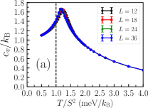
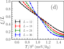
Model 2

 

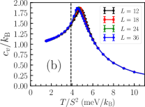
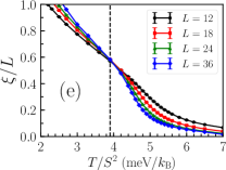
Model 3

 

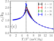
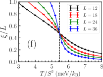
Figure 1: Specific heat $c_{v}$ (a–c) and zigzag correlation length $\xi$ (d–f) as function of temperature $T$ for Model 1 (a,d), Model 2 (b,e), and Model 3 (c,f) and different linear lattice sizes $L$. The vertical dashed line marks the position of the ordering temperature $T_{\rm N}$.

IV.2 Susceptibilties and Curie-Weiss temperatures

Model 1

 

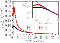
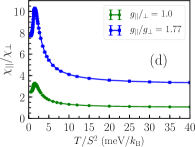
Model 2

 

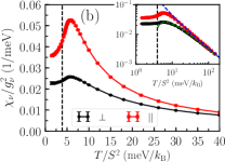
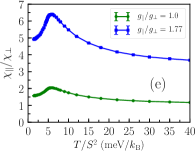
Model 3

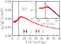
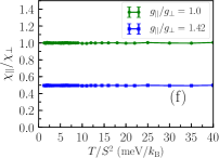
Figure 2: Out-of-plane susceptibility $\chi_{\perp}$ (black) and in-plane susceptibilities $\chi_{\parallel}$ (red) for Model 1 (a), Model 2 (b), and Model 3 (c) as function of temperature $T$. Susceptibility anisotropy ratio $\chi_{\parallel}/\chi_{\perp}$ in units of $(g_{\parallel}/g_{\perp})^{2}$ for Model 1 (d), Model 2 (e), and Model 3 (f) as function of temperature $T$. (a,b,c) MC results on an $L=24$ lattice in units of $g_{\parallel}^{2}$ and $g_{\perp}^{2}$, displaying the $g$-factor independent intrinsic anisotropy arising from the $\Gamma_{1}$ interaction in (a) and (b). Inset: Comparison between MC results (full lines) and high-temperature series expansion (dashed lines) in a log-log scale, using $c=S^{2}$. The vertical dashed line marks the position of the ordering temperature $T_{\rm N}$. (d,e,f) Susceptibility anisotropy ratio $\chi_{\parallel}/\chi_{\perp}$ for two values of the ratio $(g_{\parallel}/g_{\perp})^{2}$ from the data in (a,b,c). We considered $g_{\parallel}=2.3$ and $g_{\perp}=1.3$ (d,e) and $g_{\parallel}=1.9$ and $g_{\perp}=2.7$ (f).

From the MC data, we calculate the uniform magnetic susceptibilities as

$$\chi_{\alpha\beta}\left(T\right) = \frac{\partial M_{\alpha}}{\partial h_{\beta}}=g_{\alpha}g_{\beta}\frac{N_{\mathrm{s}}}{T}\left\langle\sigma_{\alpha}\sigma_{\beta}\right\rangle,$$ (2)

where $\left\langle\cdots\right\rangle$ denotes MC average, $M_{\alpha}=g_{\alpha}\left\langle\sigma_{\alpha}\right\rangle$ is the uniform magnetization, and $\sigma_{\alpha}=N_{\mathrm{s}}^{-1}\sum_{i}S_{i}^{\alpha}$, with $\alpha,\beta\in\{x,y,z\}$. Because the ordered state carries no uniform moment, we do not subtract the term $g_{\alpha}g_{\beta}\left\langle\sigma_{\alpha}\right\rangle\left\langle\sigma_{\beta}\right\rangle$, which we expect to go to zero in the thermodynamic limit. In the linear-response limit of Eq. (2), the $g$ factors do not enter the MC simulations directly, appearing only as prefactors.

In $\alpha$-RuCl₃, for example, the cubic axes point along nearest-neighbor Ru-Cl bonds.Janssen and Vojta (2019) For convenience, we take the crystallographic $a$ and $b$ axes along the directions $\left[11\bar{2}\right]$ and $\left[\bar{1}10\right]$, respectively, defining the honeycomb plane. The direction perpendicular to this plane is labeled as the $\left[111\right]$ direction. These three directions form a basis in which the susceptibility tensor is diagonal. Projecting Eq. (2) onto an in-plane direction then defines the in-plane susceptibility

$$\chi_{\parallel}=\chi_{zz}-\chi_{xz}.$$ (3)

Here, we have assumed that the three bond directions are equivalent, thus rendering only two independent components of the tensor susceptibility in Eq. (2): $\chi_{zz}$ and $\chi_{xz}$. Analogously, projecting the susceptibility tensor onto the $\left[111\right]$ direction perpendicular to the honeycomb layer gives the out-of-plane susceptibility

$$\chi_{\perp}=\chi_{zz}+2\chi_{xz}.$$ (4)

For an isotropic $g$ tensor, we obtain $\chi_{xz}\neq 0$ only if $\Gamma_{1}\neq 0$, and thus the anisotropy in the susceptibility can be traced back to the off-diagonal coupling $\Gamma_{1}$. In Ref. Janssen et al., 2017 it was pointed out that the $\Gamma_{1}$ term alone, without any $g$-factor anisotropy, can lead to a ratio $\chi_{\parallel}/\chi_{\perp}\sim 3-4$ at low temperatures, i.e., deep in the ordered zigzag phase. Note that these values correspond to the susceptibilities of the respective thermodynamically stable finite-field single-domain state. In $\alpha$-RuCl₃ such field-driven domain selection only happens for fields above 2 T;Banerjee et al. (2018) at smaller fields, typically all zigzag domains contribute to the susceptibility, with relative weights that depend on the sample.Lampen-Kelley et al.

IV.2.1 High-temperature expansion

To get started, it is useful to consider a high-temperature series expansion of the model in Eq. (1), which we link both to experiments and to the MC simulations. The leading correction to the Curie susceptibility is given byRau et al. (2014); Lampen-Kelley et al. (2018); Singh and Oitmaa (2017)

$$\chi_{\parallel} =g_{\parallel}^{2}\frac{c}{3T}\left(1+\frac{\Theta_{\parallel}^{{\rm CW}}}{T}\right)+\mathcal{O}(T^{-3}),$$ (5)

$$\chi_{\perp} =g_{\perp}^{2}\frac{c}{3T}\left(1+\frac{\Theta_{\perp}^{{\rm CW}}}{T}\right)+\mathcal{O}(T^{-3}),$$ (6)

with the constant

$$c=\begin{cases}S(S+1)&\text{for quantum spins},\\ S^{2}&\text{for classical spins},\end{cases}$$ (7)

and where $g_{\parallel}$ ($g_{\perp}$) is the $g$ factor along an in-plane (out-of-plane) direction. The asymptotic Curie-Weiss temperatures, defined as $\chi^{-1}_{\parallel,\perp}\left(T\right)\sim T-\Theta_{\parallel,\perp}^{\rm{CW}}+\mathcal{O}\left(T^{-1}\right)$, are given by

$$\Theta_{\parallel}^{{\rm CW}} =-\frac{c}{3}\left[3\left(J_{1}+J_{3}\right)+K_{1}-\Gamma_{1}\right],$$ (8)

$$\Theta_{\perp}^{{\rm CW}} =-\frac{c}{3}\left[3\left(J_{1}+J_{3}\right)+K_{1}+2\Gamma_{1}\right].$$ (9)

These expressions explicitly show that an intrinsic anisotropy in the model can be traced back to the $\Gamma_{1}$ term.

IV.2.2 MC results

In Figs. 2(a,b,c), we plot the out-of-plane and in-plane susceptibilities measured in the MC simulations together with the high-temperature results of Eqs. (5) and (6), using $c=S^{2}$. For Model 3, we obtain $\chi_{\parallel}=\chi_{\perp}$, Fig. 2(c), since there is no intrinsic anisotropy for $\Gamma_{1}=0$. As in the specific-heat curves in Fig. 1, the maximum in the susceptibility curves (more visible in $\chi_{\parallel}$) occurs above $T_{\rm N}$. At very high $T$ we recover Curie’s law, whereas the low-temperature susceptibilities become essentially constant as expected for an antiferromagnetic state. We find finite-size effects for this susceptibility curves to be small, and the $L=24$ result is representative of the thermodynamic behavior.

Reassuringly, the susceptibility anisotropy found at the lowest temperatures in the MC simulation, Fig. 2(a), essentially agrees with that found for the same model from $T=0$ spin-wave calculations.Janssen et al. (2017) For this comparison it is important to notice that the MC simulation, performed in the linear-response limit, averages over all zigzag domains, whereas the spin-wave calculation is performed for a particular domain. The results of both agree once domain averaging in the spin-wave calculation is properly performed.

IV.2.3 Comparison to experiments on $\alpha$-RuCl₃

For Models 1 and 2 in Table 1, which are thought to be relevant for $\alpha$-RuCl₃, we find that $\chi_{\parallel}>\chi_{\perp}$ for all temperatures we consider, with the maximum value of $(\chi_{\parallel}/g_{\parallel}^{2})/(\chi_{\perp}/g_{\perp}^{2})$ close to $3.3$ (Model 1) or $2.0$ (Model 2) in the paramagnetic regime just above $T_{\rm N}$, see Figs. 2(d,e). This is smaller than the values for $\chi_{\parallel}/\chi_{\perp}$ observed in $\alpha$-RuCl₃ experiments, indicating that either (i) the present models have to be significantly adaptedLampen-Kelley et al. (2018) or (ii) the observed magnetic anisotropy has further extrinsic contributions arising from a $g$-factor anisotropy. Since in particular Model 1 (or slight modifications thereofJanssen et al. (2020)) is found to describe well many properties of $\alpha$-RuCl₃ at low temperatures,Winter et al. (2017b); Janssen and Vojta (2019) we consider it likely that anisotropies in the $g$ factor are present due to a trigonal crystal field and should be taken into account. Further effects arising from a $\Gamma_{1}^{\prime}$ interaction are discussed in the appendix.

Previous workChaloupka and Khaliullin (2016); Yadav et al. (2016); Winter et al. (2018) suggested that $g_{\perp}\simeq 1.3$ and $g_{\parallel}\simeq 2.3$ at low $T$. In Figs. 2(d,e) we explore the effects of including these anisotropic $g$ factors, assuming that their temperature dependence is small. For Model 1 (Model 2), this gives $\chi_{\parallel}/\chi_{\perp}\approx 3.3$ $(3.7)$ at $T\simeq 40c\,\text{meV}/k_{\mathrm{B}}\simeq 350$ K for $S=1/2$. Close to the transition to the zigzag phase, we obtain $\chi_{\parallel}/\chi_{\perp}\approx 10$ $(6.4)$, whereas at low temperature $\chi_{\parallel}/\chi_{\perp}\approx 7.5$ $(5)$. Overall, Model 1 provides a satisfactory description of the experimental trend, even if the anisotropy at room temperature is too large. Part of this disagreement may be due to the fact that the single-transition samples—incidentally, those samples which agree quite well with Model 1 at low and intermediate temperatures—have a first-order structural transition between 100 K and 150 K, which has a sizeable effect on the out-of-plane susceptibility.Do et al. (2018); Lampen-Kelley et al. (2018) It is thus possible that the high-temperature phase requires a different modeling, especially of $\chi_{\perp}$. In the appendix, we demonstrate that inclusion of a small positive $\Gamma^{\prime}_{1}$ may further improve the overall agreement with the experimental data.

We note that a previous attemptLampen-Kelley et al. (2018) of fitting $\alpha$-RuCl₃ model parameters from high-temperature susceptibilities using a nearly isotropic $g$ factor Agrestini et al. (2017) yielded large values for the $\Gamma_{1}$ coupling of around $30$ meV. Since the $g$ factor enters quadratically in the susceptibility, see Eq. (2), the susceptibility anisotropy is very sensitive to a $g$-factor anisotropy. As shown above, with moderate $g$ anisotropy, the experimental data can be described with moderately large $\Gamma_{1}$.

For $T\apprge 4T_{\rm N}$, the asymptotic high-temperature expansion describes well the MC data, see insets of Figs. 2(a,b,c). The resulting anisotropic Curie-Weiss temperatures are $\Theta_{\parallel}^{{\rm CW}}=2.5c\,\text{meV}/{k_{\mathrm{B}}}$ and $\Theta_{\perp}^{{\rm CW}}=0$ (Model 1), $\Theta_{\parallel}^{{\rm CW}}=3.4c\,\text{meV}/{k_{\mathrm{B}}}$ and $\Theta_{\perp}^{{\rm CW}}=-3.2c\,\text{meV}/{k_{\mathrm{B}}}$ (Model 2). While the signs of the Curie-Weiss temperatures (mostly) agree with the experimental results,Sears et al. (2015); Majumder et al. (2015); Lampen-Kelley et al. (2018) the absolute values for $S=1/2$ as displayed in Table 1 are too small, in particular in the case of $\Theta_{\perp}^{{\rm CW}}$. As with the high-temperature susceptibility anisotropy, this discrepancy may be tied to the fact that $\chi_{\perp}$ is particularly sensitive to the first-order structural transition.

We can contrast these result with an effective Curie-Weiss temperatureSingh and Oitmaa (2017) obtained by performing a linear fit of the inverse susceptibility in a finite temperature interval, as done in experimental analyses. We choose the temperature interval $20c\,\text{meV}/k_{\mathrm{B}}\apprle T\apprle 40c\,\text{meV}/k_{\mathrm{B}}$, which corresponds to $175\,\mathrm{K}\apprle T\apprle 350\,\mathrm{K}$ for $S=1/2$, similar to the one employed in Ref. Lampen-Kelley et al., 2018. This way, we obtain $\Theta_{\parallel}^{{\rm CW}}=2.1(1)c$ meV and $\Theta_{\perp}^{{\rm CW}}=-0.3(1)c$ meV for Model 1, whereas for Model 2, we get $\Theta_{\parallel}^{{\rm CW}}=2.0(1)c$ meV and $\Theta_{\perp}^{{\rm CW}}=-4.5(1)c$ meV. Thus, the magnitude of the effective $\Theta_{\parallel}^{{\rm CW}}$ ($\Theta_{\perp}^{{\rm CW}}$) decreases (increases) with decreasing temperature. Note that the temperature dependence of the effective Curie-Weiss temperature is enhanced in Model 2, which can be traced back to the larger value of $T_{\rm N}$ in this case.

IV.2.4 Comparison to experiments on Na₂IrO₃

Without any $g$-factor anisotropy, Model 3, which was proposed as a minimal model for Na₂IrO₃, does not show any anisotropy in the susceptibility data, Fig. 2(c). However, previous susceptibility measurementsSingh and Gegenwart (2010) pointed to a significantly anisotropic $g$ factor, suggesting $g_{\perp}\simeq 2.7$ and $g_{\parallel}\simeq 1.9$. Using these estimates, the resulting susceptibilities in Model 3 are shown in Fig. 2(f). The corresponding ratio $\chi_{\parallel}/\chi_{\perp}\simeq 0.5$ roughly agrees with the experiments in Na₂IrO₃,Singh and Gegenwart (2010) supporting the view that the $\Gamma_{1}$ term is likely small in this compound.

V Effects of dilution

We now move to the evolution of the magnetic anisotropy with magnetic dilution by randomly removing a fraction $x$ of spins. Because the HK$\Gamma$ model is frustrated, we expect the combination of randomness and frustration to generically lead to a spin-glass ground state.Villain (1979); Andrade and Vojta (2014); Manni et al. (2014); Andrade et al. (2018); Aharony (1978); Imry and Ma (1975) In strictly two spatial dimensions, the freezing temperature is zero.(Maiorano and Parisi, 2018) Studying the thermodynamic glass transition thus requires a detailed description of the interlayer coupling,(Janssen et al., 2020) and we thus leave this for future work. Here, our focus will be exclusively on the disorder evolution of the uniform magnetic susceptibility and its anisotropy.

V.1 Heisenberg limit and Curie tail

Heisenberg model

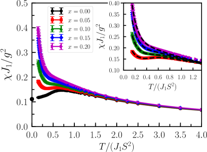
Figure 3: Uniform susceptibility $\chi$, in units of $g^{2}$, as function of temperature $T$ in the diluted Heisenberg model for different vacancy concentrations $x$, as obtained from classical MC simulations for $L=24$ and uniform $g$ factors. The black dot shows the analytical result for $x=0$ in the low-temperature limit: $\chi(x=0)=g^{2}/(9J_{1})$. Inset: Zoom into the low-temperature region with the dashed lines showing the fit given by Eq. (10).

As a warm up, let us consider the nearest-neighbor Heisenberg limit, $J_{1}>0$ and $K_{1}=\Gamma_{1}=J_{3}=0$. We then have a Néel state as ground state, while long-range order is absent for finite $T>0$. In the classical limit, the uniform susceptibility in the low-temperature limit is(Yosida, 1996) $\chi(x=0)=g^{2}/(9J_{1})+\mathcal{O}(T)$, which agrees with our numerical simulations, see black dot in Fig. 3.

As we turn on the dilution, the asymptotic Curie-Weiss temperature in Eqs. (8) and (9) is now reduced as $\Theta^{{\rm CW}}(x)=(1-x)\Theta^{{\rm CW}}(0)$, where $\Theta^{{\rm CW}}(0)=-cJ_{1}$ corresponds to the $x=0$ value, and $c=S^{2}$ [$c=S(S+1)$] for classical (quantum) spins. This is because we effectively diminish the number of neighbors of a given site.

Besides this overall suppression of the magnetic energy scale, we also observe a Curie-like tail in the low-temperature magnetic susceptibility, Fig. 3. We fit the disorder-averaged value of the susceptibility in this regime as

$$\chi(x)=g^{2}\left[x\cdot\frac{m^{2}}{T}+\left(1-x\right)\cdot\chi(0)\right],$$ (10)

where $\chi(0)$ is the low-temperature susceptibility in the clean case, and we find that $m^{2}=AS^{2}/3$, with $A$ a numerical prefactor.

This result can be rationalized as follows: A single vacancy induces a local impurity moment because the magnetization of each sublattice no longer cancel. Because the bulk magnetic order is destroyed by thermal fluctuations, the direction of this impurity moment is not fixed but is free to rotate with the local orientation of the bulk magnetic domain surrounding it, leading to a low-temperature Curie-like response at low fields.Sachdev et al. (1999); Sachdev and Vojta (2003); Höglund and Sandvik (2003); Sushkov (2003); Eggert et al. (2007); Wollny et al. (2012) Since our focus is the low-$T$ regime, for a finite concentration of impurities we are interested in the limit $\xi\gg l_{\rm imp}$, where $\xi$ is the bulk correlation length and $l_{\rm imp}\propto x^{-1/2}$ is the mean-impurity distance. In this case, the effective total impurity moment $S_{\rm eff}$ is given by the difference of the vacant sites on each sublattice: $S^{2}_{\rm eff}\sim xNS^{2}$ and we arrive at the Curie-tail contribution in Eq. (10). If we take $A\approx 2/3$, Eq. (10) fits the numerical results remarkably well for small $x$, see inset of Fig. 3. As we increase $x$, the mean impurity separation diminishes and corrections to the single-impurity result become apparent, although the leading effect is still well described by Eq. (10).

V.2 Anisotropy evolution with dilution

Model 1 Model 2 Model 3

   

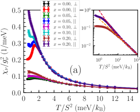
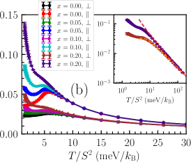
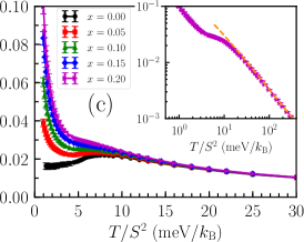
Figure 4: Uniform susceptibilities $\chi_{\nu}$, $\nu=\perp,\,\parallel$, as function of temperature $T$ in units of $g_{\perp}^{2}$ and $g_{\parallel}^{2}$, respectively, for Model 1 (a), Model 2 (b), and Model 3 (c), from classical MC simulations on an $L=24$ lattice. Insets: Susceptibilities for $x=0.20$ in a log-log scale. The dashed lines correspond to the high-temperature results, Eqs. (5) and (6).

We now investigate how the intrinsic anisotropy of the HK$\Gamma$ model evolves with random dilution. Here, the long-ranged zigzag magnetic order is destroyed for $x>0$ in favor of a spin glass in the classical limit, and we expect that the peaks in the susceptibility can no longer be associated with the onset of order, but instead mark a crossover regime below which spin fluctuations are suppressed. Actually, in $d=2$, the spin-glass order takes place onlyMaiorano and Parisi (2018) at $T=0$. Therefore, we can, in principle, expect a finite-$T$ susceptibility that resembles that of the Heisenberg limit. Our numerical results indeed indicate the presence of a Curie tail in the susceptibility, both for $\chi_{\parallel}$ and $\chi_{\perp}$. This is demonstrated in Fig. 4, which shows the susceptibilities as function of temperature for Models 1, 2, and 3.

The evolution of the anisotropy ratio $\chi_{\parallel}/\chi_{\perp}$ as function of doping $x$ for Models 1 and 2 is displayed in Fig. 5. For small doping levels, the low-temperature anisotropy increases with increasing $x$, while at the same time high-temperature anisotropy decreases. One way to rationalize this observation is to realize that the introduction of vacancies leads to an overall reduction of the exchange energy scales. Therefore, upon diluting, one effectively shifts the system to higher temperatures, which enhances the anisotropy at low temperatures, but suppresses it at high temperatures, cf. Fig. 2. For coupled layers, this increase in the susceptibility upon cooling should be bounded at low $T$ by the freezing temperature $T_{\mathrm{g}}$, and we expect this bound to be suppressed with $x$.Andrade and Vojta (2014)

Combining Eqs. (5) and  (6) with the dilution induced suppression of the Curie-Weiss temperature, $\Theta_{\parallel,\perp}^{{\rm CW}}(x)=(1-x)\Theta_{\parallel,\perp}^{{\rm CW}}(0)$, where $\Theta_{\parallel,\perp}^{{\rm CW}}(0)$ is their clean value, we obtain the high temperature disorder evolution of the susceptibilities

$$\chi_{\parallel,\perp}(x)=\chi_{\parallel,\perp}(0)-xg_{\parallel,\perp}^{2}\frac{c}{3T^{2}}\Theta_{\parallel,\perp}^{{\rm CW}}(0)+\mathcal{O}(T^{-3}),$$ (11)

where $\chi_{\parallel,\perp}(0)$ are the $x=0$ susceptibilities. As shown in the insets of Fig. 4, this equation is consistent with our numerical data. Therefore, whether disorder enhances or suppresses the high-temperature susceptibility can be traced back to the sign of the respective clean Curie-Weiss temperature. Consequently, at high temperatures, the in-plane susceptibility decreases with increasing $x$ in Models 1 and 2, while the out-of-plane susceptibility increases, at least in Model 2. This trend agrees with our simulation results, cf. Fig. 5. For Model 3, where the anisotropy is absent, we have $\Theta_{0}^{{\rm CW}}<0$, and we obtain a corresponding increase in $\chi(x)$ for increasing $x$.

Model 1 Model 2

 

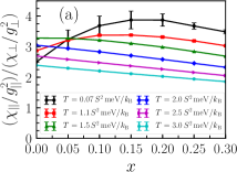
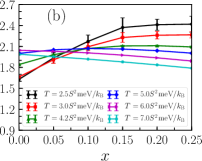
Figure 5: Susceptibility anisotropy ratio $\chi_{\parallel}/\chi_{\perp}$ in units of $(g_{\parallel}/g_{\perp})^{2}$ as function of doping level $x$ for different temperatures for Model 1 (a) and Model 2 (b), from classical MC simulations on an $L=24$ lattice. For small doping level $x$, the low-temperature anisotropy increases with increasing $x$, while its high-temperature counterpart decreases.

V.3 Comparison to experiments

V.3.1 Na₂(Ir_1-xTi_x)O₃

The diluted version of Model 3 may be relevant for Na₂(Ir_1-xTi_x)O₃. In fact, our results shown in Fig. 4(c) are broadly consistent with the reported measurements in this compound:Manni et al. (2014) (i) Upon the introduction of vacancies, the long-range order gives way to a spin glass. This glass state is identified via the separation between field-cooled and zero-field-cooled susceptibilities as measured at a very low field of 5 mT. (ii) Both the freezing temperature and the absolute value of the Curie-Weiss temperatures decrease with $x$.Manni et al. (2014); Andrade and Vojta (2014) (iii) The low-temperature part of the susceptibility is enhanced with $x$. However, the available experimental data do not address the anisotropy evolution with doping.

V.3.2 $\alpha$-(Ru_1-xIr${}_{x})$Cl₃

For $\alpha$-(Ru_1-xIr${}_{x})$Cl₃, the introduction of vacancies is accompanied by the return of two transition temperatures,Lampen-Kelley et al. (2017); Do et al. (2018) indicating the presence of stacking faults in the doped samples. These two ordering temperatures, as well as the temperature of the structural first-order phase transition, decrease with $x$. Despite the broadening of the specific-heat peak with $x$, the experimental susceptibilities show no sign of separation between field-cooled and zero-field-cooled runs. However, these susceptibility measurements were performed at comparatively high fields $\geq 100$ mT.Lampen-Kelley et al. (2017); Do et al. (2018) A weakly glassy state can therefore not be fully excluded.

The behavior of $\chi_{\parallel}$ in Model 1 as displayed in Fig. 4(a) describes qualitatively well the experimental results for $\alpha$-(Ru_1-xIr${}_{x})$Cl₃: The low-temperature increase of the in-plane susceptibility with $x$ can be linked to the impurity-induced Curie tail, whereas its decrease at high temperature can be associated with the suppression of $\Theta_{\parallel}^{{\rm CW}}$ with doping. On the other hand, the evolution of $\chi_{\perp}$ with doping in $\alpha$-(Ru_1-xIr${}_{x})$Cl₃ is more involved. Equation (11) suggests a slight increase of $\chi_{\perp}$ with doping at high temperatures, opposite to the experimental observation. Since this is a weak effect, we suspect again that the structural transition may be relevant, especially because it affects $\chi_{\perp}$ more strongly. The non-monotonic behavior of $\chi_{\perp}$ as function of $x$ at low temperatures is also not captured by our classical models: The MC results show a monotonic increase of $\chi_{\perp}$ with $x$, although it does so more slowly than $\chi_{\parallel}$.

Overall, we believe one should be very careful when comparing susceptibilities between different samples. This is because the direction-specific susceptibilities are extremely sensitive to stacking faults, which are inevitably introduced with doping.Lampen-Kelley et al. (2017) Typically, the in-plane susceptibility decreases upon the introduction of stacking faults, while at the same time the out-of-plane susceptibility increases. Lower-quality samples are therefore more isotropic than higher-quality samples.Majumder et al. (2015); Sears et al. (2015); Lampen-Kelley et al. (2018) One observable that is potentially less sample dependent is the averaged (“powder”) susceptibility $\chi_{\rm{avg}}=(2\chi_{\perp}+\chi_{\parallel})/3$, which, however, naturally lacks information about the anisotropy.

VI Conclusions and outlook

We have studied the magnetic susceptibilities in extended Heisenberg-Kitaev models, with focus on their spatial anisotropy and its evolution with temperature and magnetic dilution. We have reported results from both high-temperature expansion and large-scale classical MC simulations.

For $\alpha$-RuCl₃, our findings reconcile different results reported in the literature. We show that a set of exchange parameters, originally obtained inside the ordered phase at low temperature, describes well the behavior of the susceptibilities and their anisotropy over a large range of temperatures. This set includes a sizeable off-diagonal $\Gamma_{1}$ interaction and a moderate $g$-factor anisotropy, with the temperature dependence of the anisotropy arising solely from the $\Gamma_{1}$ interaction.

In Na₂IrO₃, the susceptibility anisotropy is mostly temperature independent, which is consistent with the assumption of a small $\Gamma_{1}$. The experimental behavior is well captured by our model, if one assumes a suitable $g$-factor anisotropy.

In the presence of doping, we find that the high-temperature susceptibilities may be mildly enhanced or suppressed depending on the sign of the clean Curie-Weiss temperature. At low temperatures, our model generically predicts the suppression of long-range order and the emergence of a spin-glass state, which agrees with the experimental observation for Na₂(Ir_1-xTi_x)O₃.Manni et al. (2014) By contrast, the experiments on $\alpha$-(Ru_1-xIr${}_{x})$Cl₃ have been interpreted in terms of a disordered spin liquid,Lampen-Kelley et al. (2017); Do et al. (2018, 2020); Baek et al. which goes beyond our semiclassical modeling. At low temperatures, we also find a Curie-tail contribution to the magnetic susceptibility, which gives rise not only an enhancement of the individual susceptibilities, but also of their anisotropy. This is in accordance with the experimental trends observed at small doping.

For $\alpha$-(Ru_1-xIr${}_{x})$Cl₃, the qualitative behavior of in-plane susceptibility $\chi_{\parallel}$ is well captured by our modeling. By contrast, the agreement for the out-of-plane susceptibility $\chi_{\perp}$ is less satisfactory. This may be linked to the presence of stacking faults, which appears to have a particularly strong influence on $\chi_{\perp}$. In this respect, a systematic study of the out-of-plane susceptibility $\chi_{\perp}$ on different $\alpha$-RuCl₃ and $\alpha$-(Ru_1-xIr${}_{x})$Cl₃ samples of varying quality would be desirable. For Na₂(Ir_1-xTi_x)O₃, we are not aware of any measurements on the anisotropy evolution, but our results for the averaged susceptibility agree well with the experiments.Manni et al. (2014)

Ideally, the evolution of the magnetic anisotropy in Kitaev materials, both with temperature and doping, could be used to further constrain the values of the symmetry allowed exchange constants, in order to complement the usual modeling in the low-temperature regime. This, however, requires more information concerning the sample dependence of the experimental behavior seen in the current data.

On the theoretical side, we have employed in this work a simple semiclassical modeling. While this approximation should yield reasonable results at intermediate and high temperatures, qualitatively new physics can emerge in the low-temperature quantum regime. This is in particular true when the ground state realizes a (disordered) Kitaev quantum spin liquid.Zschocke and Vojta (2015); Knolle et al. (2019a) While the low-doping behavior may potentially be understood in terms of isolated vacancies,Willans et al. (2010, 2011) a description of the behavior at finite doping and its temperature dependence requires a full many-body quantum computation.Nasu et al. (2015); Kimchi et al. (2018); Liu et al. (2018) This represents an excellent direction for future research.

Appendix A Trigonal distortions and $\Gamma_{1}^{\prime}$

HK$\Gamma\Gamma^{\prime}$ model

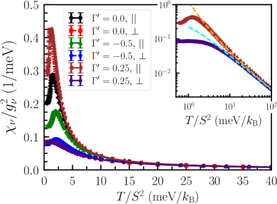
Figure 6: In-plane, $\nu=\parallel$, and out-of-plane, $\nu=\perp$, uniform magnetic susceptibilities $\chi_{\nu}$ in units of $g_{\parallel}^{2}$ and $g_{\perp}^{2}$, respectively, as function of temperature for different values of $\Gamma^{\prime}_{1}$ (in units of meV). These results were obtained from classical MC simulations on an $L=24$ lattice with $J_{1}$, $K_{1}$, $\Gamma_{1}$, and $J_{3}$ chosen as in Model 1. Inset: Susceptibilities for $\Gamma^{\prime}_{1}=0.25$ meV in a log-log scale. The dashed lines show the results from the high-temperature expansion.

The Hamiltonian presented in Eq. (1) does not contain all nearest-neighbor spin interactions that are allowed by the $C_{3}^{*}$ symmetry. This symmetry corresponds to a $2\pi/3$ spin rotation about the $\left[111\right]$ direction in spin space combined with a $2\pi/3$ lattice rotation about one site. A trigonal distortion (compression or elongation along the $\left[111\right]$ axis) fully preserves this symmetry and generates an extra nearest-neighbor magnetic couplingRau and Kee

$$\mathcal{H}^{\prime}=\Gamma_{1}^{\prime}\sum_{\left\langle ij\right\rangle_{\gamma}}\left(S_{i}^{\alpha}S_{j}^{\gamma}+S_{i}^{\beta}S_{j}^{\gamma}+S_{i}^{\gamma}S_{j}^{\alpha}+S_{i}^{\gamma}S_{j}^{\beta}\right),$$ (12)

using the same notation as in Eq. (1). For $\alpha$-RuCl₃, ab initio calculations suggest a small negative $\Gamma^{\prime}_{1}$;(Kim and Kee, 2016; Winter et al., 2016; Eichstaedt et al., 2019) however, recently it has been argued that empirical constraints require a sizeable positive $\Gamma^{\prime}_{1}$.(Maksimov and Chernyshev, 2020) We have simulated $\mathcal{H}+\mathcal{H}^{\prime}$ in the high-temperature regime to investigate the effects of $\Gamma^{\prime}_{1}$ on the magnetic anisotropy.

In Fig. 6, we show the in-plane and out-of-plane magnetic susceptibilities for different values of $\Gamma^{\prime}_{1}$. In the clean limit, we see that the anisotropy ratio $\chi_{\parallel}/\chi_{\perp}$ decreases (increases) for $\Gamma_{1}^{\prime}<0$ ($\Gamma_{1}^{\prime}>0$), resulting from a strong dependence of the in-plane susceptibility $\chi_{\parallel}$ on $\Gamma_{1}^{\prime}$ at low temperatures. Note that when $J_{1}$, $K_{1}$, $\Gamma_{1}$, and $J_{3}$ are chosen as in Model 1, the zigzag ground state is stable only up to $\Gamma^{\prime}_{1}\lesssim 0.45$ meV. For large negative $\Gamma^{\prime}_{1}\simeq-\Gamma_{1}$, the anisotropy inverts, such that $\chi_{\parallel}$ drops below $\chi_{\perp}$ in the low-temperature limit. We have checked that dilution does not alter this trend.

Inclusion of $\Gamma^{\prime}_{1}$ in the high-temperature expansion modifies the Curie-Weiss temperatures accordingly to

$$\Theta_{\parallel}^{{\rm CW}} =-\frac{c}{3}\left[3\left(J_{1}+J_{3}\right)+K_{1}-\left(\Gamma_{1}+2\Gamma_{1}^{\prime}\right)\right],$$ (13)

$$\Theta_{\perp}^{{\rm CW}} =-\frac{c}{3}\left[3\left(J_{1}+J_{3}\right)+K_{1}+2(\Gamma_{1}+2\Gamma_{1}^{\prime})\right],$$ (14)

and we show in the inset of Fig. 6 that this expression describes well the MC results at elevated temperatures.

Note that $\Gamma^{\prime}_{1}$ has a stronger influence on the low-temperature part of the anisotropy than on its high-temperature tail. This indicates that inclusion of a small positive $\Gamma^{\prime}_{1}$ may help to improve agreement with the experimental results for $\alpha$-RuCl₃. For instance, choosing $\Gamma^{\prime}_{1}=0.25$ meV and $J_{1}$, $K_{1}$, $\Gamma_{1}$, and $J_{3}$ as in Model 1, together with a slightly reduced $g$-factor anisotropy of $g_{\parallel}/g_{\perp}\simeq 1.33$, we obtain $\chi_{\parallel}/\chi_{\perp}\approx 1.9$, $8.8$, $6.2$ above room temperature, near the transition, and in the low-temperature limit, respectively. This is in well agreement with the experimental values for $\alpha$-RuCl₃.

References

- Bramwell and Gingras (2001) S. T. Bramwell and M. J. P. Gingras, Spin Ice State in Frustrated Magnetic Pyrochlore Materials, Science 294, 1495 (2001).
- Kitaev (2006) A. Kitaev, Anyons in an exactly solved model and beyond, Ann. Phys. (N.Y.) 321, 2 (2006).
- Janssen and Vojta (2019) L. Janssen and M. Vojta, Heisenberg–Kitaev physics in magnetic fields, J. Phys.: Condens. Matter 31, 423002 (2019).
- Majumder et al. (2015) M. Majumder, M. Schmidt, H. Rosner, A. A. Tsirlin, H. Yasuoka, and M. Baenitz, Anisotropic Ru3+ 4 d5 magnetism in the -RuCl3 honeycomb system: Susceptibility, specific heat, and zero-field NMR, Phys. Rev. B 91, 180401(R) (2015).
- Johnson et al. (2015) R. D. Johnson, S. C. Williams, A. A. Haghighirad, J. Singleton, V. Zapf, P. Manuel, I. I. Mazin, Y. Li, H. O. Jeschke, R. Valentí, and R. Coldea, Monoclinic crystal structure of -RuCl3 and the zigzag antiferromagnetic ground state, Phys. Rev. B 92, 235119 (2015).
- Chern et al. (2017) G.-W. Chern, Y. Sizyuk, C. Price, and N. B. Perkins, Kitaev-Heisenberg model in a magnetic field: Order-by-disorder and commensurate-incommensurate transitions, Phys. Rev. B 95, 144427 (2017).
- Rousochatzakis and Perkins (2018) I. Rousochatzakis and N. B. Perkins, Magnetic field induced evolution of intertwined orders in the Kitaev magnet , Phys. Rev. B 97, 174423 (2018).
- Das et al. (2019) S. D. Das, S. Kundu, Z. Zhu, E. Mun, R. D. McDonald, G. Li, L. Balicas, A. McCollam, G. Cao, J. G. Rau, H.-Y. Kee, V. Tripathi, and S. E. Sebastian, Magnetic anisotropy of the alkali iridate Na2IrO3 at high magnetic fields: Evidence for strong ferromagnetic Kitaev correlations, Phys. Rev. B 99, 081101(R) (2019).
- Chern et al. (2020) L. E. Chern, R. Kaneko, H.-Y. Lee, and Y. B. Kim, Magnetic field induced competing phases in spin-orbital entangled Kitaev magnets, Phys. Rev. Research 2, 013014 (2020).
- Jackeli and Khaliullin (2009) G. Jackeli and G. Khaliullin, Mott Insulators in the Strong Spin-Orbit Coupling Limit: From Heisenberg to a Quantum Compass and Kitaev Models, Phys. Rev. Lett. 102, 017205 (2009).
- Chaloupka et al. (2010) J. Chaloupka, G. Jackeli, and G. Khaliullin, Kitaev-Heisenberg Model on a Honeycomb Lattice: Possible Exotic Phases in Iridium Oxides , Phys. Rev. Lett. 105, 027204 (2010).
- Choi et al. (2012) S. K. Choi, R. Coldea, A. N. Kolmogorov, T. Lancaster, I. I. Mazin, S. J. Blundell, P. G. Radaelli, Y. Singh, P. Gegenwart, K. R. Choi, S.-W. Cheong, P. J. Baker, C. Stock, and J. Taylor, Spin Waves and Revised Crystal Structure of Honeycomb Iridate , Phys. Rev. Lett. 108, 127204 (2012).
- Singh et al. (2012) Y. Singh, S. Manni, J. Reuther, T. Berlijn, R. Thomale, W. Ku, S. Trebst, and P. Gegenwart, Relevance of the Heisenberg-Kitaev Model for the Honeycomb Lattice Iridates , Phys. Rev. Lett. 108, 127203 (2012).
- Plumb et al. (2014) K. W. Plumb, J. P. Clancy, L. J. Sandilands, V. V. Shankar, Y. F. Hu, K. S. Burch, H.-Y. Kee, and Y.-J. Kim, -RuCl3: A spin-orbit assisted Mott insulator on a honeycomb lattice, Phys. Rev. B 90, 041112(R) (2014).
- Sears et al. (2015) J. A. Sears, M. Songvilay, K. W. Plumb, J. P. Clancy, Y. Qiu, Y. Zhao, D. Parshall, and Y.-J. Kim, Magnetic order in -RuCl3: A honeycomb-lattice quantum magnet with strong spin-orbit coupling, Phys. Rev. B 91, 144420 (2015).
- Baek et al. (2017) S.-H. Baek, S.-H. Do, K.-Y. Choi, Y. S. Kwon, A. U. B. Wolter, S. Nishimoto, J. van den Brink, and B. Büchner, Evidence for a Field-Induced Quantum Spin Liquid in -RuCl3, Phys. Rev. Lett. 119, 037201 (2017).
- Wolter et al. (2017) A. U. B. Wolter, L. T. Corredor, L. Janssen, K. Nenkov, S. Schönecker, S.-H. Do, K.-Y. Choi, R. Albrecht, J. Hunger, T. Doert, M. Vojta, and B. Büchner, Field-induced quantum criticality in the Kitaev system -RuCl3, Phys. Rev. B 96, 041405(R) (2017).
- Sears et al. (2017) J. A. Sears, Y. Zhao, Z. Xu, J. W. Lynn, and Y.-J. Kim, Phase diagram of -RuCl3 in an in-plane magnetic field, Phys. Rev. B 95, 180411(R) (2017).
- Gass et al. (2020) S. Gass, P. M. Cônsoli, V. Kocsis, L. T. Corredor, P. Lampen-Kelley, D. G. Mandrus, S. E. Nagler, L. Janssen, M. Vojta, B. Büchner, and A. U. B. Wolter, Field-induced phase transitions of the Kitaev material -RuCl3 probed by thermal expansion and magnetostriction, Phys. Rev. B 101, 245158 (2020).
- (20) S. Bachus, D. A. S. Kaib, Y. Tokiwa, A. Jesche, V. Tsurkan, A. Loidl, S. M. Winter, A. A. Tsirlin, R. Valenti, and P. Gegenwart, Thermodynamic perspective on the field-induced behavior of -RuCl3, arXiv:2006.02428 .
- Banerjee et al. (2016) A. Banerjee, C. A. Bridges, J.-Q. Yan, A. A. Aczel, L. Li, M. B. Stone, G. E. Granroth, M. D. Lumsden, Y. Yiu, J. Knolle, S. Bhattacharjee, D. L. Kovrizhin, R. Moessner, D. A. Tennant, D. G. Mandrus, and S. E. Nagler, Proximate Kitaev quantum spin liquid behaviour in a honeycomb magnet, Nature Mat. 15, 733 (2016).
- Banerjee et al. (2018) A. Banerjee, P. Lampen-Kelley, J. Knolle, C. Balz, A. A. Aczel, B. Winn, Y. Liu, D. Pajerowski, J. Yan, C. A. Bridges, A. T. Savici, B. C. Chakoumakos, M. D. Lumsden, D. A. Tennant, R. Moessner, D. G. Mandrus, and S. E. Nagler, Excitations in the field-induced quantum spin liquid state of -RuCl3, npj Quantum Materials 3, 8 (2018).
- Kasahara et al. (2018) Y. Kasahara, T. Ohnishi, Y. Mizukami, O. Tanaka, S. Ma, K. Sugii, N. Kurita, H. Tanaka, J. Nasu, Y. Motome, T. Shibauchi, and Y. Matsuda, Majorana quantization and half-integer thermal quantum Hall effect in a Kitaev spin liquid, Nature 559, 227 (2018).
- Kitagawa et al. (2018) K. Kitagawa, T. Takayama, Y. Matsumoto, A. Kato, R. Takano, Y. Kishimoto, S. Bette, R. Dinnebier, G. Jackeli, and H. Takagi, A spin-orbital-entangled quantum liquid on a honeycomb lattice, Nature 554, 341 (2018).
- Knolle et al. (2019a) J. Knolle, R. Moessner, and N. B. Perkins, Bond-Disordered Spin Liquid and the Honeycomb Iridate : Abundant Low-Energy Density of States from Random Majorana Hopping, Phys. Rev. Lett. 122, 047202 (2019a).
- Lampen-Kelley et al. (2017) P. Lampen-Kelley, A. Banerjee, A. A. Aczel, H. B. Cao, M. B. Stone, C. A. Bridges, J. Q. Yan, S. E. Nagler, and D. Mandrus, Destabilization of Magnetic Order in a Dilute Kitaev Spin Liquid Candidate, Phys. Rev. Lett. 119, 237203 (2017).
- (27) S.-H. Baek, H. W. Yeo, S.-H. Do, K. Y. Choi, L. Janssen, M. Vojta, and B. Büchner, Observation of a gapless spin liquid in a diluted Kitaev honeycomb material, arXiv:2005.139836 .
- Takagi et al. (2019) H. Takagi, T. Takayama, G. Jackeli, G. Khaliullin, and S. E. Nagler, Concept and realization of Kitaev quantum spin liquids, Nat. Rev. Phys. 1, 264 (2019).
- Do et al. (2018) S.-H. Do, W. J. Lee, S. Lee, Y. S. Choi, K. J. Lee, D. I. Gorbunov, J. Wosnitza, B. J. Suh, and K.-Y. Choi, Short-range quasistatic order and critical spin correlations in -Ru1-xIrxCl3, Phys. Rev. B 98, 014407 (2018).
- Do et al. (2020) S.-H. Do, C. H. Lee, T. Kihara, Y. S. Choi, S. Yoon, K. Kim, H. Cheong, W.-T. Chen, F. Chou, H. Nojiri, and K.-Y. Choi, Randomly Hopping Majorana Fermions in the Diluted Kitaev System -Ru0.8Ir0.2Cl3, Phys. Rev. Lett. 124, 047204 (2020).
- Manni et al. (2014) S. Manni, Y. Tokiwa, and P. Gegenwart, Effect of nonmagnetic dilution in the honeycomb-lattice iridates Na2IrO3 and Li2IrO3, Phys. Rev. B 89, 241102(R) (2014).
- Kubota et al. (2015) Y. Kubota, H. Tanaka, T. Ono, Y. Narumi, and K. Kindo, Successive magnetic phase transitions in -RuCl3: XY-like frustrated magnet on the honeycomb lattice, Phys. Rev. B 91, 094422 (2015).
- (33) For small fields, i.e., in the linear-response limit, the susceptibility is identical for all in-plane directions provided that the three honeycomb bonds are equivalent.
- Lampen-Kelley et al. (2018) P. Lampen-Kelley, S. Rachel, J. Reuther, J.-Q. Yan, A. Banerjee, C. A. Bridges, H. B. Cao, S. E. Nagler, and D. Mandrus, Anisotropic susceptibilities in the honeycomb Kitaev system -RuCl3, Phys. Rev. B 98, 100403(R) (2018).
- (35) P. Lampen-Kelley, L. Janssen, E. C. Andrade, S. Rachel, J.-Q. Yan, C. Balz, D. G. Mandrus, S. E. Nagler, and M. Vojta, Field-induced intermediate phase in -RuCl3: Non-coplanar order, phase diagram, and proximate spin liquid, arXiv:1807.06192 .
- Cao et al. (2016) H. B. Cao, A. Banerjee, J. Q. Yan, C. A. Bridges, M. D. Lumsden, D. G. Mandrus, D. A. Tennant, B. C. Chakoumakos, and S. E. Nagler, Low-temperature crystal and magnetic structure of -RuCl3, Phys. Rev. B 93, 134423 (2016).
- Janssen et al. (2020) L. Janssen, S. Koch, and M. Vojta, Magnon dispersion and dynamic spin response in three-dimensional spin models for -RuCl3, Phys. Rev. B 101, 174444 (2020).
- Singh and Gegenwart (2010) Y. Singh and P. Gegenwart, Antiferromagnetic Mott insulating state in single crystals of the honeycomb lattice material Na2IrO3, Phys. Rev. B 82, 064412 (2010).
- (39) In Ref. Singh and Gegenwart, 2010, the susceptibilities along the crystallographic axis and an axis perpendicular to have been measured, which in the structure of Na2IrO3 only approximately agrees with axes perpendicular and parallel to the honeycomb plane.
- Manni (2014) S. Manni, Synthesis and investigation of frustrated Honeycomb lattice iridates and rhodates, Ph.D. thesis, Georg-August-Universität Göttingen (2014).
- Rau et al. (2014) J. G. Rau, E. K.-H. Lee, and H.-Y. Kee, Generic Spin Model for the Honeycomb Iridates beyond the Kitaev Limit, Phys. Rev. Lett. 112, 077204 (2014).
- Glamazda et al. (2017) A. Glamazda, P. Lemmens, S.-H. Do, Y. S. Kwon, and K.-Y. Choi, Relation between kitaev magnetism and structure in , Phys. Rev. B 95, 174429 (2017).
- Reschke et al. (2017) S. Reschke, F. Mayr, Z. Wang, S.-H. Do, K.-Y. Choi, and A. Loidl, Electronic and phonon excitations in , Phys. Rev. B 96, 165120 (2017).
- Janssen et al. (2017) L. Janssen, E. C. Andrade, and M. Vojta, Magnetization processes of zigzag states on the honeycomb lattice: Identifying spin models for -RuCl3 and Na2IrO3, Phys. Rev. B 96, 064430 (2017).
- (45) J. G. Rau and H.-Y. Kee, Trigonal distortion in the honeycomb iridates: Proximity of zigzag and spiral phases in na2iro3, arXiv:1408.4811 .
- Winter et al. (2016) S. M. Winter, Y. Li, H. O. Jeschke, and R. Valentí, Challenges in design of Kitaev materials: Magnetic interactions from competing energy scales, Phys. Rev. B 93, 214431 (2016).
- Ran et al. (2017) K. Ran, J. Wang, W. Wang, Z.-Y. Dong, X. Ren, S. Bao, S. Li, Z. Ma, Y. Gan, Y. Zhang, J. T. Park, G. Deng, S. Danilkin, S.-L. Yu, J.-X. Li, and J. Wen, Spin-Wave Excitations Evidencing the Kitaev Interaction in Single Crystalline -RuCl3, Phys. Rev. Lett. 118, 107203 (2017).
- Winter et al. (2017a) S. M. Winter, K. Riedl, P. A. Maksimov, A. L. Chernyshev, A. Honecker, and R. Valentí, Breakdown of magnons in a strongly spin-orbital coupled magnet, Nat. Comm. 8, 1152 (2017a).
- Sizyuk et al. (2014) Y. Sizyuk, C. Price, P. Wölfle, and N. B. Perkins, Importance of anisotropic exchange interactions in honeycomb iridates: Minimal model for zigzag antiferromagnetic order in , Phys. Rev. B 90, 155126 (2014).
- Sizyuk et al. (2016) Y. Sizyuk, P. Wölfle, and N. B. Perkins, Selection of direction of the ordered moments in Na2IrO3 and -RuCl3, Phys. Rev. B 94, 085109 (2016).
- Katukuri et al. (2014) V. M. Katukuri, S. Nishimoto, V. Yushankhai, A. Stoyanova, H. Kandpal, S. Choi, R. Coldea, I. Rousochatzakis, L. Hozoi, and J. van den Brink, Kitaev interactions between moments in honeycomb Na2IrO3 are large and ferromagnetic: insights from ab initio quantum chemistry calculations, New J. Phys. 16, 013056 (2014).
- Price and Perkins (2012) C. C. Price and N. B. Perkins, Critical Properties of the Kitaev-Heisenberg Model, Phys. Rev. Lett. 109, 187201 (2012).
- Price and Perkins (2013) C. Price and N. B. Perkins, Finite-temperature phase diagram of the classical Kitaev-Heisenberg model, Phys. Rev. B 88, 024410 (2013).
- José et al. (1977) J. V. José, L. P. Kadanoff, S. Kirkpatrick, and D. R. Nelson, Renormalization, vortices, and symmetry-breaking perturbations in the two-dimensional planar model, Phys. Rev. B 16, 1217 (1977).
- Andrade and Vojta (2014) E. C. Andrade and M. Vojta, Magnetism in spin models for depleted honeycomb-lattice iridates: Spin-glass order towards percolation, Phys. Rev. B 90, 205112 (2014).
- Chaloupka and Khaliullin (2015) J. Chaloupka and G. Khaliullin, Hidden symmetries of the extended Kitaev-Heisenberg model: Implications for the honeycomb-lattice iridates , Phys. Rev. B 92, 024413 (2015).
- Chaloupka and Khaliullin (2016) J. Chaloupka and G. Khaliullin, Magnetic anisotropy in the Kitaev model systems Na2IrO3 and -RuCl3, Phys. Rev. B 94, 064435 (2016).
- Iino et al. (2019) S. Iino, S. Morita, N. Kawashima, and A. W. Sandvik, Detecting Signals of Weakly First-order Phase Transitions in Two-dimensional Potts Models, J. Phys. Soc. Jpn. 88, 034006 (2019).
- Singh and Oitmaa (2017) R. R. P. Singh and J. Oitmaa, High-temperature thermodynamics of the honeycomb-lattice Kitaev-Heisenberg model: A high-temperature series expansion study, Phys. Rev. B 96, 144414 (2017).
- Winter et al. (2017b) S. M. Winter, A. A. Tsirlin, M. Daghofer, J. van den Brink, Y. Singh, P. Gegenwart, and R. Valentí, Models and materials for generalized kitaev magnetism, J. Phys.: Condens. Matter 29, 493002 (2017b).
- Yadav et al. (2016) R. Yadav, N. A. Bogdanov, V. M. Katukuri, S. Nishimoto, J. van den Brink, and L. Hozoi, Kitaev exchange and field-induced quantum spin-liquid states in honeycomb -RuCl3, Sci. Rep. 6, 37925 (2016).
- Winter et al. (2018) S. M. Winter, K. Riedl, D. Kaib, R. Coldea, and R. Valentí, Probing -RuCl3 Beyond Magnetic Order: Effects of Temperature and Magnetic Field, Phys. Rev. Lett. 120, 077203 (2018).
- Agrestini et al. (2017) S. Agrestini, C.-Y. Kuo, K.-T. Ko, Z. Hu, D. Kasinathan, H. B. Vasili, J. Herrero-Martin, S. M. Valvidares, E. Pellegrin, L.-Y. Jang, A. Henschel, M. Schmidt, A. Tanaka, and L. H. Tjeng, Electronically highly cubic conditions for Ru in -RuCl3, Phys. Rev. B 96, 161107(R) (2017).
- Villain (1979) J. Villain, Insulating spin glasses, Z. Phys. B 33, 31 (1979).
- Andrade et al. (2018) E. C. Andrade, J. A. Hoyos, S. Rachel, and M. Vojta, Cluster-Glass Phase in Pyrochlore Antiferromagnets with Quenched Disorder, Phys. Rev. Lett. 120, 097204 (2018).
- Aharony (1978) A. Aharony, Absence of Ferromagnetic Long Range Order in Random Isotropic Dipolar Magnets and in similar systems, Solid State Commun. 28, 667 (1978).
- Imry and Ma (1975) Y. Imry and S. Ma, Random-Field Instability of the Ordered State of Continuous Symmetry, Phys. Rev. Lett. 35, 1399 (1975).
- Maiorano and Parisi (2018) A. Maiorano and G. Parisi, Support for the value 5/2 for the spin glass lower critical dimension at zero magnetic field, Proc. Natl. Acad. Sci. USA 115, 5129 (2018).
- Yosida (1996) K. Yosida, Theory of Magnetism (Springer, Berlin, 1996).
- Sachdev et al. (1999) S. Sachdev, C. Buragohain, and M. Vojta, Quantum Impurity in a Nearly Critical Two-Dimensional Antiferromagnet, Science 286, 2479 (1999).
- Sachdev and Vojta (2003) S. Sachdev and M. Vojta, Quantum impurity in an antiferromagnet: Nonlinear sigma model theory, Phys. Rev. B 68, 064419 (2003).
- Höglund and Sandvik (2003) K. H. Höglund and A. W. Sandvik, Susceptibility of the 2D Spin- Heisenberg Antiferromagnet with an Impurity, Phys. Rev. Lett. 91, 077204 (2003).
- Sushkov (2003) O. P. Sushkov, Long-range dynamics related to magnetic impurities in the two-dimensional Heisenberg antiferromagnet, Phys. Rev. B 68, 094426 (2003).
- Eggert et al. (2007) S. Eggert, O. F. Syljuåsen, F. Anfuso, and M. Andres, Universal Alternating Order around Impurities in Antiferromagnets, Phys. Rev. Lett. 99, 097204 (2007).
- Wollny et al. (2012) A. Wollny, E. C. Andrade, and M. Vojta, Singular Field Response and Singular Screening of Vacancies in Antiferromagnets, Phys. Rev. Lett. 109, 177203 (2012).
- Zschocke and Vojta (2015) F. Zschocke and M. Vojta, Physical states and finite-size effects in Kitaev’s honeycomb model: Bond disorder, spin excitations, and NMR line shape, Phys. Rev. B 92, 014403 (2015).
- Willans et al. (2010) A. J. Willans, J. T. Chalker, and R. Moessner, Disorder in a Quantum Spin Liquid: Flux Binding and Local Moment Formation, Phys. Rev. Lett. 104, 237203 (2010).
- Willans et al. (2011) A. J. Willans, J. T. Chalker, and R. Moessner, Site dilution in the Kitaev honeycomb model, Phys. Rev. B 84, 115146 (2011).
- Nasu et al. (2015) J. Nasu, M. Udagawa, and Y. Motome, Thermal fractionalization of quantum spins in a Kitaev model: Temperature-linear specific heat and coherent transport of Majorana fermions, Phys. Rev. B 92, 115122 (2015).
- Kimchi et al. (2018) I. Kimchi, A. Nahum, and T. Senthil, Valence Bonds in Random Quantum Magnets: Theory and Application to YbMgGaO4, Phys. Rev. X 8, 031028 (2018).
- Liu et al. (2018) L. Liu, H. Shao, Y.-C. Lin, W. Guo, and A. W. Sandvik, Random-Singlet Phase in Disordered Two-Dimensional Quantum Magnets, Phys. Rev. X 8, 041040 (2018).
- Kim and Kee (2016) H.-S. Kim and H.-Y. Kee, Crystal structure and magnetism in -RuCl3: An ab initio study, Phys. Rev. B 93, 155143 (2016).
- Eichstaedt et al. (2019) C. Eichstaedt, Y. Zhang, P. Laurell, S. Okamoto, A. G. Eguiluz, and T. Berlijn, Deriving models for the Kitaev spin-liquid candidate material -RuCl3 from first principles, Phys. Rev. B 100, 075110 (2019).
- Maksimov and Chernyshev (2020) P. A. Maksimov and A. L. Chernyshev, Rethinking , Phys. Rev. Research 2, 033011 (2020).