Exceptional Spin Liquids from Couplings to the Environment

Abstract

We establish the appearance of a qualitatively new type of spin liquid with emergent exceptional points when coupling to the environment. We consider an open system of the Kitaev honeycomb model generically coupled to an external environment. In extended parameter regimes, the Dirac points of the emergent Majorana fermions from the original model are split into exceptional points with Fermi arcs connecting them. In glaring contrast to the original gapless phase of the honeycomb model which requires time-reversal symmetry, this new phase is stable against all perturbations. The system also displays a large sensitivity to boundary conditions resulting from the non-Hermitian skin effect with telltale experimental consequences. Our results point to the emergence of new classes of spin liquids in open systems which might be generically realized due to unavoidable couplings with the environment.

Quantum spin liquids are low-temperature phases of matter with fractionalized excitations and emergent gauge fields ANDERSON (1987); Balents (2010); Savary and Balents (2016); Knolle and Moessner (2019); Broholm et al. (2020). Efforts at identifying possible spin liquids has led to hundreds of candidates due to the various possible symmetries present in lattice systems. However, a broader view of the nature of the fractionalized excitations and gauge field leads to only a few prominent types Balents (2010), some of which are realized in exactly solvable models Kitaev (2003, 2006); Levin and Wen (2005); Yao and Kivelson (2007); Schroeter et al. (2007); Mandal and Surendran (2009); Chua et al. (2011); Morampudi et al. (2014); Buerschaper et al. (2014). Here, we show that coupling a spin liquid to an environment can lead to a qualitatively new kind of phase which cannot occur in any closed system.

Dissipative systems can display unusual phenomenology not seen in closed systems. These range from unusual phase transitions and critical phases Horstmann et al. (2013); Matsumoto et al. (2019); Xiao et al. (2019); Hanai and Littlewood (2020) to new topological phases Bergholtz et al. (2019); Gong et al. (2018); Cerjan et al. (2019); Zhou et al. (2018). One prominent class of phenomena can be understood in regimes where a non-Hermitian description Bergholtz et al. (2019); Gong et al. (2018); Yao et al. (2018); Budich et al. (2019); Bergholtz and Budich (2019); Zhang et al. (2019); Kawabata et al. (2019); Lee (2016) of the system is appropriate. This allows for the appearance of exceptional points (EPs) in the spectrum when two eigenvectors coincide Berry (2004); Ding et al. (2016); Park et al. (2020); Miri and Alù (2019). In non-interacting systems, band crossings with such exceptional points result in an unconventional square-root dispersion at low energies as opposed to a typical Dirac dispersion as seen in graphene. These band crossings in 2D systems are generic unlike the accidental symmetry-protected crossings in graphene Bergholtz et al. (2019); Zhou et al. (2018). The conventional bulk-boundary correspondence is also shown to be broken due to an exotic non-Hermitian skin effect Yao and Wang (2018); Kunst et al. (2018); Xiong (2018); Xiao et al. (2020); Schomerus (2020); Ghatak et al. (2019); Helbig et al. (2020); Yoshida et al. (2019a), which results in localization of all eigenstates at the boundary. This results in an exponential sensitivity of the system to boundary conditions. Based on work of free systems, interest is now drawn to understanding effects in interacting systems Yoshida et al. (2019b); Lee (2020); Matsumoto et al. (2019); Liu et al. (2020); Carlström (2020); Shackleton and Scheurer (2020); Liu et al. (2020); Yoshida et al. (2020a). It is natural to ask what novel features can appear when a system possessing internal strong correlation is described by such an effective non-Hermitian Hamiltonian.

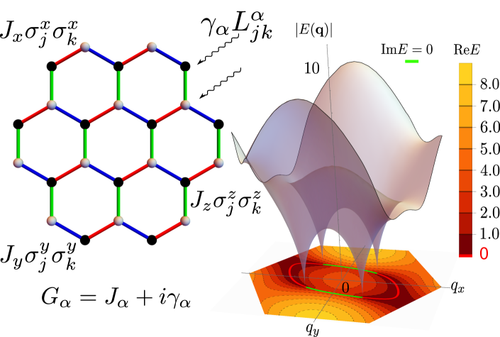
Figure 1: Left: The lattice of the Kitaev honeycomb model. The spins are coupled through $J_{\alpha}\sigma^{\alpha}_{j}\sigma^{\alpha}_{k}(\alpha=x,y,z)$. The coupling to the environment is described by jump operators $L^{\alpha}_{jk}$. Right: the 3D spectrum diagram for the non-Hermitian Kitaev honeycomb model at $G_{x}=2,G_{y}=1,G_{z}=2.5\exp(i\pi/3)$. The Fermi arc ($\textrm{Re}E=0$) is labelled with the red line and the green line indicates the $\textrm{Im}E=0$ curve.

In this Letter we show that these phenomena can be realized in an interacting spin model giving rise to a qualitatively new kind of spin liquid. We illustrate this by coupling the Kitaev honeycomb model Kitaev (2006) to an environment (Fig. 1, left panel). In certain regimes, the two Dirac points generically split into four exceptional points (Fig. 1, right panel). The four exceptional points are paired up with each pair connected through Fermi arcs reminiscent to those found in Weyl semimetals Armitage et al. (2018), but occurring in the bulk rather than on the boundaries of the system. Unlike the closed system where the ferromagnetic spin liquid and the anti-ferromagnetic spin liquid are separated by a nodal-line critical point, the open system can go from one to the other by splitting and recombination of exceptional points. Moreover, the only way to produce a gap is to bring the exceptional points together, again similar to Weyl points in 3D. Thus the coupling to the environment elevates a symmetry protected gapless spin liquid to a generically stable phase which we term an exceptional spin liquid. We also show the occurrence of the skin effect on open zig-zag boundaries leading to a large sensitivity on boundary conditions. Finally, we show that the phenomena are naturally expected to arise in potential realizations of the honeycomb model, such as those proposed in cold atoms and ion traps.

Model

- The Kitaev honeycomb model Kitaev (2006) is defined through compass interactions linking directions in spin space and real space of spin-$1/2$:

$$H_{0}=-\sum_{\langle jk\rangle_{\alpha}}J_{\alpha}\sigma^{\alpha}_{j}\sigma^{\alpha}_{k},$$ (1)

where $\langle jk\rangle_{\alpha}$ labels the lattice (Fig. 1) and $\alpha=x,y,z$ labelling the three types of links of a hexagonal lattice with $\sigma^{\alpha}$ the corresponding Pauli matrices.

We consider an open system where the Kitaev Hamiltonian is coupled to an environment. The resulting open system is described by a Lindblad master equation Lindblad (1976) for the density matrix

$$\frac{d}{dt}\rho=-i[H_{0},\rho]+\sum_{\langle jk\rangle_{\alpha}}\gamma_{\alpha}\left(L_{jk}^{\alpha}\rho L_{jk}^{\alpha\dagger}-\frac{1}{2}\left\{L_{jk}^{\alpha\dagger}L_{jk}^{\alpha},\rho\right\}\right),$$ (2)

where $L_{jk}^{\alpha}$ are jump operators describing how the system is coupled to the bath and we have set $\hbar=1$. The dynamics can be interpreted in terms of deterministic evolution of a trajectory (wavefunction) described by an effective non-Hermitian Hamiltonian $H_{\rm NH}=H_{0}-(i/2)\sum_{\langle jk\rangle_{\alpha}}\gamma_{\alpha}L^{\alpha\dagger}_{jk}L_{jk}^{\alpha}$, interspersed with quantum jumps to different states through the $L_{jk}^{\alpha}\rho L_{jk}^{\alpha\dagger}$ term Dum et al. (1992); Mølmer et al. (1993); Plenio and Knight (1998); Daley (2014). Thus when we are measuring at times before the first jump, the dynamics is governed by the non-Hermitian Hamiltonian $H_{\rm NH}$. This can be interpreted as a measurement backaction in settings where realizations of the model system are post-selected to consider only cases where the jump has not occurred Plenio and Knight (1998); Daley (2014); Lee and Chan (2014); Ashida et al. (2016); Nakagawa et al. (2020).

Although the general phenomenology of what follows is largely independent of the form of the jump operators, we consider here jump operators $L_{jk}^{\alpha}=\sigma_{j}^{\alpha}+\sigma_{k}^{\alpha}$ along each each $\alpha$-type link $j-k$ for illustration. Similar results can be obtained by considering the effect of dephasing noise Shibata and Katsura (2019). This results in an effective non-Hermitian description of the the form of Eq. (1) but with the coupling constants being complex and henceforth labeled by $G_{\alpha}=J_{\alpha}+i\gamma_{\alpha}$. This model is exactly solved through an enlarged Majorana representation of the spin operators. Introducing four Majorana fermions $(c_{j},b_{j}^{x},b_{j}^{y},b_{j}^{z})$ at each site, the spin is represented as $\sigma_{j}^{\alpha}=ic_{j}b_{j}^{a}$. The physical state is constrained by the condition: $D_{j}|\textrm{phys}\rangle=|\textrm{phys}\rangle$, with $D_{j}=b^{x}_{j}b^{y}_{j}b^{z}_{j}c_{j}$. Defining bond operators $u_{jk}=ib_{j}^{\alpha}b_{k}^{\alpha}$, where $\alpha$ is the type of link $j-k$, the effective model is

$$H_{\rm NH}=-\sum_{\langle jk\rangle_{\alpha}}G_{\alpha}\sigma^{\alpha}_{j}\sigma^{\alpha}_{k}=i\sum_{\langle jk\rangle_{\alpha}}G_{\alpha}u_{jk}c_{j}c_{k}\ .$$ (3)

The bond operator $u_{jk}$ is a constant of motion in the enlarged Majorana representation. Meanwhile, a physical conserved quantity is the product of $u_{jk}$ around a plaquette $p$, $W_{p}=\prod_{j-k\in p}u_{jk}$. The eigenvectors can thus be grouped into different sectors of the eigenvalues $W_{p}=\pm 1$. The sector with all $W_{p}=1$ is viewed as vortex free and $W_{p}=-1$ means a $\mathbb{Z}_{2}$-vortex at $p$.

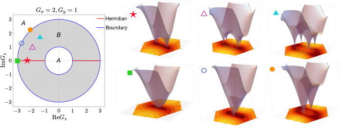
Figure 2: The spectrum and phase diagram for the non-Hermitian Kitaev honeycomb model at $G_{x}=2,G_{y}=1$. The grey region $B$ admits band-touching points while the region $A$ possesses a (complex) gap. Six values of $G_{z}$ are taken to exhibit different dispersions with respect to $\mathbf{q}$ as in Fig. 1. For the Hermitian situation (the star), around the band-touching point $E\sim\sqrt{g_{\alpha\beta}\delta q_{\alpha}\delta q_{\beta}}$ with coefficients $g_{\alpha\beta}$. At the Hermitian phase boundary (the square), the dispersion is quadratic along a certain direction $E\sim\sqrt{(g_{\alpha}\delta q_{\alpha})^{4}}$ with coefficients $g_{\alpha}$. In the non-Hermitian situation (the two triangles), the dispersion is square-root $E\sim\sqrt{g^{\prime}_{\alpha}\delta q_{\alpha}}$. At the non-Hermitian boundary (the two circles), the energy is linear along some direction $E\sim\sqrt{g^{\prime}_{\alpha\beta}\delta q_{\alpha}\delta q_{\beta}}$.

The eigenstates of the model can be decomposed into different $\mathbb{Z}_{2}$-flux sectors as in the original Hermitian model, where the zero-flux is the relevant one at low (real) energies due to Lieb’s theorem Kitaev (2006); Lieb (1994). In fact, the zero-flux sector is still relevant for the open systems in appropriate regimes where all the phenomenology we discuss is realized. To illustrate this, consider the Hermitian model at temperatures much lower than the vison gap. If we consider multiplying it by an overall complex number, there is a parametric separation in lifetimes of states between different flux sectors and the zero-flux sector corresponds to states with the longest lifetimes. In the supplementary material we provide numerical evidence that this holds true also in more general cases sup .

In the zero-flux sector we can chose $u_{jk}=1$ for $j$ on one sublattice and $k$ on the other. The Hamiltonian becomes a tight binding Majorana model, in momentum space as:

$$\widetilde{H}=\sideset{}{{}^{\prime}}{\sum}_{\mathbf{q}}\left(\begin{array}[]{ccc}c_{-\mathbf{q},1}&c_{-\mathbf{q},2}\end{array}\right)\left(\begin{array}[]{ccc}0&iA(\mathbf{q})\\ -iA(-\mathbf{q})&0\end{array}\right)\left(\begin{array}[]{ccc}c_{\mathbf{q},1}\\ c_{\mathbf{q},2}\end{array}\right),$$ (4)

where in the primed summation $\sideset{}{{}^{\prime}}{\sum}$ we count the pair $\mathbf{q},-\mathbf{q}$ only once. This is because $c_{-\mathbf{q}}=c^{\dagger}_{\mathbf{q}}$. The off-diagonal element is $A(\mathbf{q})=2\left(G_{x}e^{i\mathbf{q}\cdot\mathbf{r}_{1}}+G_{y}e^{i\mathbf{q}\cdot\mathbf{r}_{2}}+G_{z}\right)$ and the subscripts $1,2$ label the two sublattices of the honeycomb system. The momentum-space operators satisfy $\{c_{\mathbf{q},\lambda},c_{-\mathbf{q}^{\prime},\gamma}\}=\delta_{\mathbf{q},\mathbf{q}^{\prime}}\delta_{\lambda,\gamma}$. Depending on whether $A(\mathbf{q})$ can go to zero, the system exhibits a gapped or a gapless phases. In the Hermitian model, the gapped phase is equivalent to a toric code spin liquid Kitaev (2003) while the gapless phase can possess non-Abelian statistics in the presence of magnetic field Kitaev (2006). The gapless condition is given that the lengths $|G_{x}|,|G_{y}|,|G_{z}|$ admit a triangle:

$$|G_{x}|\leq|G_{y}|+|G_{z}|,\ |G_{y}|\leq|G_{x}|+|G_{z}|,\ |G_{z}|\leq|G_{x}|+|G_{y}|.$$ (5)

Exceptional points and Fermi arcs

- The spectrum is obtained by the eigenvectors of the matrix (4) $E^{2}(\mathbf{q})=A(\mathbf{q})A(-\mathbf{q})$. In the Hermitian case, there are two Dirac points inside the gapless region. We show that for complex $G_{\alpha}$, the band touching points have a square-root dispersion and are exceptional points.

For convenience of computation here, we can extract out the phase of $G_{z}$ as an overall phase of $\widetilde{H}$, so the Hamiltonian is now parameterized by $\bar{\phi}_{x}=\phi_{x}-\phi_{z},\bar{\phi}_{y}=\phi_{y}-\phi_{z}$. In the Brillouin zone, it is more convenient to parametrize as $\mathbf{q}=\mathbf{q}_{1}\tilde{q}_{1}/(2\pi)+\mathbf{q}_{2}\tilde{q}_{2}/(2\pi)$, where $\mathbf{q}_{1}$ and $\mathbf{q}_{2}$ are the reciprocal lattice vectors. The values $\tilde{q}_{1},\tilde{q}_{2}$ uniquely fix the vector $\mathbf{q}$ (notice that we should take $\tilde{q}_{1},\tilde{q}_{2}\textrm{ mod }2\pi$). Zero energy at $\mathbf{q}$ implies $A(\mathbf{q})=0$ or $A(-\mathbf{q})=0$. The $A(\mathbf{q})=0$ condition gives $\tilde{q}_{1},\tilde{q}_{2}$

$$\tilde{q}_{1(2)}=\pm\cos^{-1}\left(\frac{|G_{y(x)}|^{2}-|G_{z}|^{2}-|G_{x(y)}|^{2}}{2|G_{x(y)}||G_{z}|}\right)-\bar{\phi}_{x(y)}$$ (6)

with the constraint $G_{x}\sin(\tilde{q}_{1}+\bar{\phi}_{x})=-G_{y}\sin(\tilde{q}_{2}+\bar{\phi}_{y})$ to fix the $\pm$ signs above. These equations admit at most two solutions which we denote them as $\mathbf{q}_{e},\mathbf{q}^{\prime}_{e}$. In the Hermitian situation, one has $A^{*}(\mathbf{q})=A(-\mathbf{q})$ and $\mathbf{q}_{e}=-\mathbf{q}^{\prime}_{e}$ as $\bar{\phi}_{x}=\bar{\phi}_{y}=0$. Linearizing $A$ it directly follows that we have Dirac points with a conventional linear dispersion away from the degeneracies.

For complex, i.e., non-Hermitian, parameters, we have $A^{*}(\mathbf{q})\neq A(-\mathbf{q})$ and $\mathbf{q}_{e}=-\mathbf{q}^{\prime}_{e}-2(\bar{\phi}_{x},\bar{\phi}_{y})$. Now $A(\mathbf{q})$ and $A(-\mathbf{q})$ vanish at different points, implying four $E=0$ exceptional points $\pm\mathbf{q}_{e},\pm\mathbf{q}^{\prime}_{e}$, at which the Hamiltonian matrix becomes non-diagonalizable and the two eigenvectors coincide. The dispersion near the exceptional points takes a square-root form instead of the conic form since $A(\mathbf{q})$ and $A(-\mathbf{q})$ do not vanish simultaneously. The $\textrm{Re}E=0$ branch cuts associated with the square-roots have a natural interpretation as bulk Fermi arcs, and the exceptional points are connected by these Fermi arcs and their imaginary counterparts $\textrm{Im}E=0$ (cf. Fig. 1, right panel).

When the coupling constants are tuned out of the triangle regime Eq. (5), the four exceptional points fuse into two exceptional points and then disappears. A cut at $G_{x}=2,G_{y}=1$ for different complex $G_{z}$ is shown in Fig. 2, where we also plot the absolute energy $|E|$ and its real part, ${\rm Re}E$, at different $G_{z}$. One can see the splitting of each Hermitian band-touching point into two non-Hermitian exceptional points. At the phase boundary, the branch-cut for $E$ disappears. In this situation, the band-touching point is not protected and thus gets gapped out when crossing the phase boundary. This illustrates how, similar to Weyl points in 3D, the exceptional points can only be gapped out when combined pairwise, in glaring contrast to the 2D Dirac points that are inherently symmetry protected.

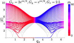
(a)

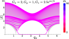
(b)

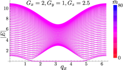
(c)

Figure 3: The spectra of the system for OBC (colored) and PBC (light gray) and the corresponding average localization of the eigenstates. (a) A non-Hermitian skin effect occuring due to the non-trivial relative phase $\phi_{x}-\phi_{y}\neq 0\ (\textrm{mod }\pi)$. (b) The skin effect does not occur if only $G_{z}$ is tuned complex while $\phi_{x}-\phi_{y}=0\ (\textrm{mod }\pi)$. (c) The Hermitian case, where the PBC and OBC spectra overlap except for the edge mode. All results are obtained for a $M=80$-row lattice.

Skin effects

- Boundary conditions do not affect the spectrum for Hermitian systems in the thermodynamic limit except for additional edge states. In contrast, non-Hermitian systems display a strong sensitivity to boundary conditions. To illustrate this, we consider Eq. (3) with two parallel zigzag boundaries. We place the open boundary condition (OBC) perpendicular to the $z$-type link, which is along the $y$-direction. The $x$-direction is still chosen to be periodic with $N_{x}$ unit cells. For convenience of comparison with the periodic boundary condition (PBC), the number of layers sandwiched by the two boundaries is taken to be even $M=4M^{\prime}$. The Hamiltonian is diagonal in the momentum $q_{x}$ and we denote the state by $\psi(m)$ with $m$ the layer index. The boundary conditions require $\psi(0)=0$ and $\psi(M+1)=0$. The question can be solved by a transfer matrix method Kunst and Dwivedi (2019); sup . We group the wave functions into a doublet $\Psi(m)=(\psi(2m),\psi(2m+1))$. Then the equation of motion takes the form $\Psi(m)=T\Psi(m-1)$, where $T$ is the transfer matrix (details in sup ). Each eigenstate $\Psi(m)$ can be therefore constructed as a superposition of the two eigenvectors of $T$, $\Psi(m)=\alpha s_{1}^{m}\Psi_{1}+\beta s_{2}^{m}\Psi_{2}$ with $\Psi_{1,2}$ the eigenvectors of $T$ and $s_{1,2}$ the corresponding eigenvalues, such that it satisfies $\psi(0)=\psi(M+1)=0$. If we consider Hermitian couplings, then $|s_{1}|=|s_{2}|=1$ and the eigenstates propagate into the bulk. However in the non-Hermitian situation, $s_{1}\simeq s_{2}$ are either both larger or smaller than one and the states are piled up against one of the boundaries. This is known as the non-Hermitian skin effects Yao and Wang (2018); Kunst et al. (2018). The general criterion for the skin effect is when $|s_{1}s_{2}|$ given by

$$|\det T|=\frac{\left|G_{x}e^{iq_{x}a}+G_{y}\right|}{\left|G_{x}e^{-iq_{x}a}+G_{y}\right|}\neq 1.$$ (7)

In this case, all eigenstates are exponentially localized to the boundary $\psi(m)\sim\exp(-m/l)$, with $l=(\ln|\det T|)/2$. We see that this occurs when the relative phase $\phi_{x}-\phi_{y}$ is non-zero. By rotation symmetry, we can draw the conclusion that for two parallel zigzag open boundaries perpendicular to $\alpha$-type links, the skin effects can be turned on by giving a non-trivial relative phase $\phi_{\beta}-\phi_{\gamma}$, where $\beta,\gamma\neq\alpha$.

In Fig. 3a-3c, we show the OBC spectra for different constants. The average localization of the wave function, $\bar{m}=\sum m|\psi(m)|^{2}$, is indicated with the color plot. For a non-vanishing $\phi_{x}-\phi_{y}$, as in Fig. 3a, in addition to the zero-energy boundary state, the bulk states are also piling up the $m=1$ boundary, exhibiting the skin effects. The localization shift from one boundary to the other at $q_{x}=0,\pi$, in accordance with Eq. (7). The spectrum is strikingly different from the PBC spectrum. For a vanishing $\phi_{x}-\phi_{y}$ and non-vanishing $\phi_{z}$, we can however see in Fig. 3b that there is no skin effect despite the presence of bulk exceptional points and the OBC spectrum coincide with the PBC spectrum. Fig. 3c shows a Hermitan example contrasting the novel non-Hermitian behaviour.

Discussion

- We have shown in this Letter that genuinely non-Hermitian phenomenology, exceptional points and skin effects, intriguingly conspire with fractionalization in the interacting Kitaev honeycomb model in dissipative environments. This results in a qualitatively new type of non-equilibrium matter which we call exceptional spin liquids, which is by its dissipative nature, lies beyond earlier classification schemes and potentially displays new dynamics beyond current spin liquids Knolle et al. (2014); Morampudi et al. (2017); Werman et al. (2018); Morampudi et al. (2020). Remarkably, this new phase is generic in the sense that it does not rely on any underlying symmetries—this may in fact greatly facilitate the prospects for observing gapless spin liquids in synthetic setups.

The exceptional points can naturally arise in many of the proposed realizations of the Kitaev honeycomb model Duan et al. (2003); Micheli et al. (2007); Jackeli and Khaliullin (2009); Schmied et al. (2011); You et al. (2010); Gorshkov et al. (2013). Two concrete mechanisms involve incorporating effects of a self-energy Yoshida et al. (2020b) and a post-selection procedure Plenio and Knight (1998); Daley (2014); Ashida et al. (2016); Naghiloo et al. (2019) on synthetic realizations. The material candidates for the Kitaev honeycomb model could potentially realize this non-Hermitian phenomenology if the effects of excitations such as phonons are taken into account. Here, we expound on the post-selection procedure in a synthetic optical lattice systems of ultracold atoms. Such systems are unavoidably subject to dissipative effects, most notably from spontaneous emission and inelastic collisions Bloch et al. (2008); Riou et al. (2012). As mentioned above (Eq. 2), the absence of quantum jumps from such processes leads to a measurement backaction Plenio and Knight (1998); Daley (2014); Lee and Chan (2014); Ashida et al. (2016); Nakagawa et al. (2020) resulting in a non-Hermitian evolution. If spontaneous emission is the dominant dissipative mechanism, the procedure is implemented by a continuous measurement of the system to monitor for emitted photons and a post-selection on those realizations where no photons are observed.

Considering ${}^{87}\mathrm{Rb}$ atoms with a typical magnetic scale of 100 Hz, the scattering rate due to spontaneous emission is a few Hz. It is dependent on the detuning $\Delta$ of the laser as $\Delta^{-2}$ and can hence be tuned appropriately across a wide range from milliseconds to many minutes Friebel et al. (1998). Further tuning can be achieved by using different transitions in the same or different atoms since the spontaneous emission rate goes as $\omega_{0}^{3}$ where $\omega_{0}$ is the transition energy. The losses due to inelastic collisions can also be tuned through techniques such as external confinement, Feshbach resonance and photoassociation Bloch et al. (2008). The Kitaev honeycomb model can be realized with hyperfine states and a spin-dependent potential Duan et al. (2003). Using different detunings for the different lasers creating the lattice can then result in the direction-dependent Lindblad operators necessary for the phenomenology here. Although it would seem beneficial to have a detuning which is as large as possibles since that would lead to a bigger separation of the exceptional points, it is practically limited by the transition frequency. More importantly, it also make the post-selection procedure more difficult since the Poissonian decay process means that the probability of a decay not occuring would be $\sim e^{-N\gamma/\delta}$ where $\gamma$ is the noise rate, $N$ is the number of spins and $\delta$ is the imaginary part of the many-body gap. Hence, the primary challenge would be to resolve the exceptional points due to a small separation. Choosing parameters such that the zero-flux sector has the longest lifetime (see Supplementary) would give an enhancement to the naive lifetime and might allow one to choose larger noise rates to better resolve the exceptional points.

The exquisite control and ubiquitous presence of dissipation in the suggested synthetic implementations of our ideas might even open the door for novel technological applications such ultra sensitive sensing devices based on harnessing the non-Hermitian skin effect Budich and Bergholtz (2020) by judiciously manipulating the boundary conditions.

As strongly correlated many-body states exhibit a rich variety of emergent phenomena, such as non-Abelian statistics, the study of their interplay with genuinely non-Hermitian effects as advanced here is likely to provide fertile ground for new fundamental discoveries.

I Supplemental Material

II Band touching points

We give an exhaustive result for the properties of band touching points in this part. We illustrate how the exceptional points split and fuse into the Dirac points.

First we identify the nature of the band touching point. We focus on non-zero $G_{\alpha}$. The energy is given by $E(\mathbf{q})=\pm\sqrt{A(\mathbf{q})A(-\mathbf{q})}$. In the Hermitian case, $A(-\mathbf{q})=A^{\ast}(\mathbf{q})$, the dispersion must be at least linear around the band touching point. In the non-Hermtian case, $A(-\mathbf{q})\neq A^{\ast}(\mathbf{q})$ in general. The dispersion is usually square-root dependent around the band-touching point. In fact, if $A(-\mathbf{q})=A^{\ast}(\mathbf{q})=0$, then we can find that $G_{x}\sin(\tilde{q}_{1})=-G_{y}\sin(\tilde{q}_{2})$. This requires either $\phi_{x}=\phi_{y}$ (mod $\pi$) or the band-touching point at the inversion-invariant point ($\tilde{q}_{1},\tilde{q}_{2}=0,\pi$). In the first situation, for simplicity we can absorb the phases $\phi_{x}$ and $\phi_{y}$ into $\phi_{z}$. Using $\textrm{Im}A(\mathbf{q})=\textrm{Im}A(-\mathbf{q})=0$, we obtain $G_{x}\sin(\tilde{q}_{1})+G_{y}\sin(\tilde{q}_{2})+|G_{z}|\sin{\phi_{z}}=0$ and $-G_{x}\sin(\tilde{q}_{1})-G_{y}\sin(\tilde{q}_{2})+|G_{z}|\sin{\phi_{z}}=0$. So $\phi_{z}=0$ (mod $\pi$), all $G_{\alpha}$ have to share the same phase and the system is simply obtained by the Hermtian one times an overall phase. In the second situation where the band-touching points are at the inversion-invariant points, i.e. $\tilde{q}_{1},\tilde{q}_{2}=0,\pi$, we as before absorb the phase of $G_{z}$ into the overall phase of the Hamiltonian. The band-touching condition is:

$$|G_{x}|\cos(\tilde{q}_{1}+\bar{\phi}_{x})+|G_{y}|\cos(\tilde{q}_{2}+\bar{\phi}_{y})+G_{z}=0,\quad|G_{x}|\sin(\tilde{q}_{1}+\bar{\phi}_{x})+|G_{y}|\sin(\tilde{q}_{2}+\bar{\phi}_{y})=0.$$ (S1)

From these two equations, one finds that

$$|G_{x}|=\frac{\sin(\bar{\phi}_{y}+\tilde{q}_{2})}{\sin(\bar{\phi}_{x}+\tilde{q}_{1}-\bar{\phi}_{y}-\tilde{q}_{2})}|G_{z}|,\quad|G_{y}|=\frac{\sin(\bar{\phi}_{x}+\tilde{q}_{1})}{\sin(\bar{\phi}_{y}+\tilde{q}_{2}-\bar{\phi}_{x}-\tilde{q}_{1})}|G_{z}|.$$ (S2)

This means we need a fine tuning to have the band-touching point located at the inversion-invariant point. Therefore, we conclude that the band-touching point is Dirac-like only for Hermitian Hamiltonians up to an overall complex phase or fine tuning where the band-touching point takes place at the inversion-invariant point in the Brillouin zone. Otherwise, the band-touching points possess a defect Hamiltonian and are exceptional points.

Then we consider the boundary between the gapless phase $B$ and the gapped phase $A$ when the Hamiltonian is non-Hermitian. We rewrite the band-touching condition as

$$\cos(\tilde{q}_{1}+\bar{\phi}_{x})=\frac{|G_{y}|^{2}-|G_{z}|^{2}-|G_{x}|^{2}}{2|G_{x}||G_{z}|},\quad\cos(\tilde{q}_{2}+\bar{\phi}_{y})=\frac{|G_{x}|^{2}-|G_{z}|^{2}-|G_{y}|^{2}}{2|G_{y}||G_{z}|},$$ (S3)

$$|G_{x}|\sin(\tilde{q}_{1}+\bar{\phi}_{x})+|G_{y}|\sin(\tilde{q}_{2}+\bar{\phi}_{y})=0.$$ (S4)

The boundary is reached when the solution to Eq. (S3) is at its extremes. That is, $|\cos(\tilde{q}_{1}+\bar{\phi}_{x})|=1$ or $|\cos(\tilde{q}_{2}+\bar{\phi}_{y})|=1$ in Eq. (S3). According to Eq. (S4), we actually have $|\cos(\tilde{q}_{1}+\bar{\phi}_{x})|=|\cos(\tilde{q}_{2}+\bar{\phi}_{y})|=1$. In this situation, there is only one solution to $A(\mathbf{q})=0$. For the Hermitian situation, this means the two Dirac points appearing in pairs $\mathbf{q}_{\ast},-\mathbf{q}_{\ast}$ are fusing into one. For general non-Hermitian case, according to the discussion in the above paragraph, the band-touching point $\mathbf{q}_{e}$ is usually not inversion invariant. So we obtain two exceptional points at the phase boundary $,\mathbf{q}_{e},-\mathbf{q}_{e}$. We conclude that in general when the non-Hermitian system is evolving from the gappless to gapped phase, the four exceptional points fuse into two and then get gapped out.

We give the form of the Hamiltonian near the band-touching point. The Hamiltonian can be parameterized by the Pauli matrix as

$$H=\frac{A(\mathbf{q})+A(-\mathbf{q})}{2}\sigma_{x}+\frac{A(\mathbf{q})-A(-\mathbf{q})}{2}i\sigma_{y}.$$ (S5)

For an Hermitian Hamiltonian, $A(-\mathbf{q})=A^{\ast}(\mathbf{q})$. At the Dirac point $\mathbf{q}_{\ast}$, we have $A(\mathbf{q})\simeq g_{\alpha}\delta q_{\alpha}$, where $g_{\alpha}$ is a complex vector and $\delta\mathbf{q}=\mathbf{q}-\mathbf{q}_{\ast}$. So the Hamiltonian takes the form $H=\sigma_{x}\delta q_{\alpha}\textrm{Re }g_{\alpha}-\sigma_{y}\delta q_{\alpha}\textrm{Im }g_{\alpha}$. In general $\textrm{Re }g_{\alpha}$ and $\textrm{Im }g_{\alpha}$ are linearly independent. So the dispersion of the energy is linear $E\simeq\sqrt{g_{\alpha}g^{\ast}_{\beta}\delta q_{\alpha}\delta q_{\beta}}$. At the Hermitian phase boundary, using $\mathbf{q}_{\ast}=-\mathbf{q}_{\ast}$, one can deduce that $\textrm{Re }g_{\alpha}=0$ and $g_{\alpha}q_{\alpha}=0$. So the Hamiltonian becomes $H=ig_{\alpha}\delta_{\alpha}\sigma_{y}$ and $E\sim|\delta\mathbf{q}|^{2}$ for $\delta\mathbf{q}$ perpendicular to $\textrm{Im }g_{\alpha}$. In the non-Hermtian situation, at the band touching point only one of $A(\mathbf{q}),A(-\mathbf{q})$ vanishes. Let’s take $A(\mathbf{q}_{e})=0$ and $A(\mathbf{q})\simeq g_{\alpha}\delta q_{\alpha}$. Then the Hamiltonian and the energy are expressed as

$$H\simeq\left(\begin{array}[]{ccc}0&g_{\alpha}\delta q_{\alpha}\\ A(-\mathbf{q}_{e})&0\end{array}\right),\quad E\simeq\sqrt{A(-\mathbf{q}_{e})g_{\alpha}\delta q_{\alpha}}.$$ (S6)

As before, the real and the imaginary part of $g_{\alpha}$ are usually linearly independent. The energy is square-root dependent on $\delta q$. At the gap-gapless boundary, by examining the structure of Eq. (S1) as done in the last paragraph, the vector $g_{\alpha}$ is real up to a complex phase. In that case, along the orthogonal direction to $g_{\alpha}$, the dispersion $E(\mathbf{q})$ is linear in $\delta q$.

Another interesting feature compared to the Hermitian situation is how the system can evolve from ferromagnetic couplings to anti-ferromagnetic couplings. We notice that the Majoranas are agnostic to whether the coupling is ferromagnetic or anti-ferromagnetic, and only depends on the modulus $|G_{\alpha}|$. However, in the Hermitian case, we have to pass through the $G_{\alpha}=0$ point, which is equivalent to an array of $1$D gapless chains. Below we list how the exceptional points and the Fermi arcs evolves when $\phi_{z}$ going from $0$ to $\pi$ at fixed $G_{x}=2,G_{y}=1$ in Fig. S1. From ferromagnetic $G_{z}$ coupling to anti-ferromagnetic $G_{z}$ coupling, one can observe that there are two recombination processes of the Fermi arc. Two Fermi arcs appear in splitting each Dirac point to two exceptional points. Between $\phi_{z}=\pi/4$ and $\phi_{z}=5\pi/12$, the two Fermi arcs collide for the first time. How they connect the four exceptional points into two pairs changes. Each Fermi arc together with their imaginary counterpart winds over the torus hole, forming a closed path that can not shrink into a point. Between $\phi_{z}=7\pi/12$ to $\phi_{z}=3\pi/4$, the Fermi arcs collide again. This time the Fermi arcs again connect the exceptional points in the same way as for small $\phi_{z}$. And they eventually diminish when $\phi_{z}$ is approaching $\pi$. In summary, in the non-Hermitian situation, we can go from a anti-ferromagnetic Kitaev spin liquid $J_{\alpha}<0$ to an ferromagnetic Kitaev spin liquid $J_{\alpha}>0$ by splitting and reconnecting exceptional points. While in the Hermitian case, one has to go through the critical regime $J_{\alpha}=0$ exhibiting nodal lines. The non-Hermitian coupling thus provides paths circumventing this critical point.

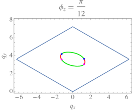
(a)

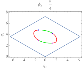
(b)

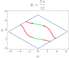
(c)

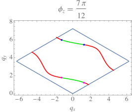
(d)

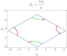
(e)

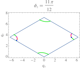
(f)

Figure S1: (a)-(f) The evolution of the band-touching points, Fermi arcs (red) and the $\textrm{Im}E=0$ curve (green) for $G_{x}=2,G_{y}=1$ and $G_{z}=2.5\exp(i\phi_{z})$ from $\phi_{z}=\pi/12$ to $\phi_{z}=11\pi/12$.

III The transfer matrix solution to open boundary condition

Now we solve the OBC problem. The Hamiltonian is diagonal in momentum $q_{x}$. We do the Fourier transformation of the Majorana operators as $c_{q_{x},m}=\sum_{n}(1/\sqrt{2N_{x}})c_{n,m}e^{-iq_{x}n}$. The Hamiltonian then takes the form $\widetilde{H}=\sum_{m,m^{\prime},q_{x}}A^{O}_{m,n}(q_{x})c_{-q_{x},m}c_{q_{x},m^{\prime}}$, where the matrix $A^{O}$ is given by

$$A^{O}=\begin{pmatrix}0&ir(q_{x})&\ &\ &\ &\ &\ \\ -ir^{\prime}(q_{x})&0&it&\ &\ &\ &\ \\ \ &-it^{\prime}&0&ir(q_{x})&\ &\ &\ \\ \ &\ &-ir^{\prime}(q_{x})&0&it&\ &\ \\ \ &\ &\ &\ddots&\ddots&\ddots&\ \end{pmatrix},$$ (S7)

where $r(q_{x})=r^{\prime}(-q_{x})=2\left[G_{x}e^{-iq_{x}a/2}+G_{y}e^{iq_{x}a/2}\right]$ and $t=t^{\prime}=-2G_{z}$.

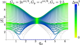
(a)

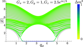
(b)

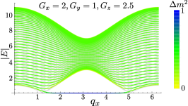
(c)

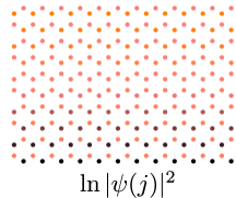
(d)

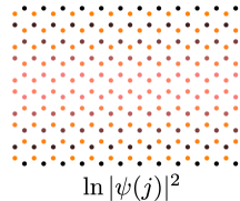
(e)

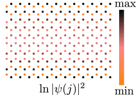
(f)

Figure S2: The spectra for OBC (colored) and PBC (light gray) and the corresponding localisation variance of the state. The calculation is performed on a $M=80$-row lattice (a) The skin effect situation. (b) No skin effect exhibits when only $G_{z}$ is tuned complex. The zero-mode edge state is performed on a slightly smaller OBC lattice. (c) The Hermitian result, also with the zero-mode edge computed on a slightly smaller OPC lattice. (d)-(f) The corresponding logarithmic distribution of the wave functions $\ln|\psi(j)\psi(j)|$ on the lattice at $q_{x}=2\pi/3$.

We use the transfer matrix to analyze the eigenstates $\psi(m)$ of the above matrix. Like in the main text, we rewrite them as a doublet $\Psi(m)=(\psi(2m),\psi(2m+1))$. The eigenstate equation becomes

$$T_{+}\Psi(m)+T_{-}\Psi(m-1)=0,\quad\Rightarrow\Psi(m)=T\Psi(m-1),$$ (S8)

where those transfer matrices are given by

$$T_{+}=\left(\begin{array}[]{ccc}ir&0\\ -E&it\end{array}\right),\quad T_{-}=\left(\begin{array}[]{ccc}-it^{\prime}&-E\\ 0&-ir^{\prime}\end{array}\right),\quad T=-T_{+}^{-1}T_{-}=\frac{1}{tr}\left(\begin{array}[]{ccc}tt^{\prime}&-itE\\ -it^{\prime}E&rr^{\prime}-E^{2}\end{array}\right).$$ (S9)

In order to find the solution for OPB, we need to compute $T^{M/2}$, which is convenient by transforming $T$ into a diagonal matrix through a similarity transformation:

$$T=P\left(\begin{array}[]{ccc}s_{1}&0\\ 0&s_{2}\end{array}\right)P^{-1},\quad s_{1},s_{2}=\frac{1}{2tr}\left[rr^{\prime}+tt^{\prime}-E^{2}\mp\sqrt{(rr^{\prime}-tt^{\prime}-E^{2})^{2}-4tt^{\prime}E^{2}}\right].$$ (S10)

where $P$ is formed by the columns of the right eigenvectors of $T$ and $P^{-1}$ is formed by the rows of the left eigenvectors of $T$. The boundary condition now can be written as:

$$P\left(\begin{array}[]{ccc}s_{1}^{M/2}&0\\ 0&s_{2}^{M/2}\end{array}\right)P^{-1}\left(\begin{array}[]{ccc}0\\ \psi(1)\end{array}\right)=\left(\begin{array}[]{ccc}\psi(M)\\ 0\end{array}\right)\Rightarrow\left(\begin{array}[]{ccc}A\left(s_{1}^{M/2}-s_{1}^{M/2}\right)\\ Bs_{1}^{M/2}+(1-B)s_{2}^{M/2}\end{array}\right)\psi(1)=\left(\begin{array}[]{ccc}\psi(M)\\ 0\end{array}\right),$$ (S11)

where the values $A,B$ are given by

$$A=\frac{it}{\sqrt{(rr^{\prime}-tt^{\prime}-E^{2})^{2}-4tt^{\prime}E^{2}}},\quad B=\frac{1}{2}-\frac{rr^{\prime}-tt^{\prime}-E^{2}}{2\sqrt{(rr^{\prime}-tt^{\prime}-E^{2})^{2}-4tt^{\prime}E^{2}}}.$$ (S12)

The energy is solved by the implicit equation $Bs_{1}^{M/2}+(1-B)s_{2}^{M/2}=0$. In the large-$M$ limit, $|s_{1}/s_{2}|=|(1-B)/B|^{2/M}$. This value goes to $1$ if neither $B$ nor $1-B$ vanishes, which requires $E\neq 0$. Therefore for a state with finite $|E|$, we can deduce $|s_{1}|\simeq|s_{2}|$. The distribution of the bulk state is thus derived as in the main text as $|s_{1}|\simeq|s_{2}|\simeq\sqrt{|\det T|}$. In Ref. Kunst and Dwivedi (2019), the authors show that in order to obtain a dense spectrum in the $M\to\infty$ limit, one should have $|s_{1}|=|s_{2}|$. States with $|s_{1}|\neq|s_{2}|$ are exceptional and treated as boundary states.

In figure S2, we plot the average square position $\Delta m^{2}=\sum[m-(M+1)/2]^{2}|\psi(m)|^{2}$ and the distribution of the wave function on the real-space lattice.

IV Two-vortex sector

Figure S3: The energy of a series of two-vortex configurations at $J_{x}=J_{y}=\exp(-0.2i),J_{z}=\exp(-0.3i)$.

We numerically compute the energy of the two-vortex sector to demonstrate that it is possible to have the zero-flux sector equipped with a longer lifetime.

In order to realize this, we first put an overall phase to the Hamiltonian so that the zero-flux sector has the longest lifetime. Then we add a non-trivial non-Hermitian perturbation. The calculation is performed on a torus of $50\times 50$ unit cells with periodic boundary condition.

Inside each vortex sector, there are a macroscopic number of states. When the Hamiltonian is Hermitian, the most relevant state in each sector is the one with the lowest energy. For a non-Hermitian Hamiltonian, usually we have a state with the lowest energy and a different state with the longest lifetime. If we consider a non-Hermitian perturbation and a short-time evolution compared to the lifetime, the most relevant procedures come from the excitation to higer-energy states. In this case, it is reasonable to consider the lowest-energy state inside each vortex sector. The energy of the two-vortex configuration is then given by summing all the Majorana states with negative $\textrm{Re}E$. This gives the usual definition of the ground state, the state with lowest $\textrm{Re}E$. One difference here is that finite-size effects can be very large. This is because it possible to have Majorana states with small $\textrm{Re}E$ but big $\textrm{Im}E$. They lead to a large oscillation in the imaginary part of the two-vortex energy. In order to justify a finite-size calculation, we have to limit ourselves to very small non-Hermitian couplings. In our tentative numerical calculation, we find that only at very extremely small non-Hermitian perturbations, $\phi_{\alpha}<0.05$, can the finite-size effect be completely removed. This leads to very small separation between EPs. Nevertheless, for a slightly larger $\phi_{\alpha}$, we still have a zero-flux sector with a longer lifetime despite finite-size effects.

We compute the all two-vortex configurations on a $25\times 25$ quarter of the torus at $J_{x}=J_{y}=\exp(-0.2i),J_{z}=\exp(-0.3i)$. We verified that all these configurations have a shorter lifetime and higher energy than the vortex-free configuration. Some of the configuration are presented in Fig. S3. The energy difference between the two-vortex configuration and the zero-vortex sector has a positive $\textrm{Re}\Delta E$ so that the zero-vortex sector is the ground state. The imaginary part $\textrm{Im}\Delta E$ is negative. This guarantees that $\exp(-i\Delta Et)$ is a decaying factor and all two-vortex configurations decays faster than the zero-vortex sector. In Fig. S4, we list the energy of the two-vortex configuration with respect to the vortex distance. One see for $J_{x}=J_{y}=\exp(-0.2i),J_{z}=\exp(-0.3i)$, there is still a jump in $\textrm{Im }E$. Such an irregularity disappears for $J_{x}=J_{y}=\exp(-0.05i),J_{z}=\exp(-0.1i)$

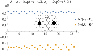
(a)

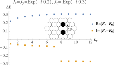
(b)

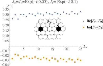
(c)

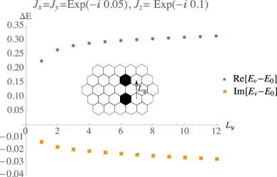
(d)

Figure S4: The energy of the two-vortex configuration as a function of the vortex distance $L_{x},L_{y}$.

References

- ANDERSON (1987) P. W. ANDERSON, “The resonating valence bond state in la2cuo4 and superconductivity,” Science 235, 1196–1198 (1987).
- Balents (2010) L. Balents, “Spin liquids in frustrated magnets,” Nature 464, 199 (2010).
- Savary and Balents (2016) L. Savary and L. Balents, “Quantum spin liquids: a review,” Reports on Progress in Physics 80, 016502 (2016).
- Knolle and Moessner (2019) J. Knolle and R. Moessner, “A field guide to spin liquids,” Annual Review of Condensed Matter Physics 10, 451–472 (2019).
- Broholm et al. (2020) C. Broholm, R. J. Cava, S. A. Kivelson, D. G. Nocera, M. R. Norman, and T. Senthil, “Quantum spin liquids,” Science 367 (2020), 10.1126/science.aay0668.
- Kitaev (2003) A. Kitaev, “Fault-tolerant quantum computation by anyons,” Annals of Physics 303, 2 – 30 (2003).
- Kitaev (2006) A. Kitaev, “Anyons in an exactly solved model and beyond,” Annals of Physics 321, 2 – 111 (2006), january Special Issue.
- Levin and Wen (2005) M. A. Levin and X.-G. Wen, “String-net condensation: A physical mechanism for topological phases,” Phys. Rev. B 71, 045110 (2005).
- Yao and Kivelson (2007) H. Yao and S. A. Kivelson, “Exact chiral spin liquid with non-abelian anyons,” Phys. Rev. Lett. 99, 247203 (2007).
- Schroeter et al. (2007) D. F. Schroeter, E. Kapit, R. Thomale, and M. Greiter, “Spin hamiltonian for which the chiral spin liquid is the exact ground state,” Phys. Rev. Lett. 99, 097202 (2007).
- Mandal and Surendran (2009) S. Mandal and N. Surendran, “Exactly solvable kitaev model in three dimensions,” Phys. Rev. B 79, 024426 (2009).
- Chua et al. (2011) V. Chua, H. Yao, and G. A. Fiete, “Exact chiral spin liquid with stable spin fermi surface on the kagome lattice,” Phys. Rev. B 83, 180412 (2011).
- Morampudi et al. (2014) S. C. Morampudi, C. von Keyserlingk, and F. Pollmann, “Numerical study of a transition between z 2 topologically ordered phases,” Phys. Rev. B 90, 035117 (2014).
- Buerschaper et al. (2014) O. Buerschaper, S. C. Morampudi, and F. Pollmann, “Double semion phase in an exactly solvable quantum dimer model on the kagome lattice,” Phys. Rev. B 90, 195148 (2014).
- Horstmann et al. (2013) B. Horstmann, J. I. Cirac, and G. Giedke, “Noise-driven dynamics and phase transitions in fermionic systems,” Phys. Rev. A 87, 012108 (2013).
- Matsumoto et al. (2019) N. Matsumoto, K. Kawabata, Y. Ashida, S. Furukawa, and M. Ueda, “Continuous phase transition without gap closing in non-hermitian quantum many-body systems,” arXiv preprint arXiv:1912.09045 (2019).
- Xiao et al. (2019) L. Xiao, K. Wang, X. Zhan, Z. Bian, K. Kawabata, M. Ueda, W. Yi, and P. Xue, “Observation of critical phenomena in parity-time-symmetric quantum dynamics,” Phys. Rev. Lett. 123, 230401 (2019).
- Hanai and Littlewood (2020) R. Hanai and P. B. Littlewood, “Critical fluctuations at a many-body exceptional point,” Phys. Rev. Research 2, 033018 (2020).
- Bergholtz et al. (2019) E. J. Bergholtz, J. C. Budich, and F. K. Kunst, “Exceptional topology of non-hermitian systems,” arXiv preprint arXiv:1912.10048 (2019).
- Gong et al. (2018) Z. Gong, Y. Ashida, K. Kawabata, K. Takasan, S. Higashikawa, and M. Ueda, “Topological phases of non-hermitian systems,” Phys. Rev. X 8, 031079 (2018).
- Cerjan et al. (2019) A. Cerjan, S. Huang, M. Wang, K. P. Chen, Y. Chong, and M. C. Rechtsman, “Experimental realization of a weyl exceptional ring,” Nature Photonics 13, 623–628 (2019).
- Zhou et al. (2018) H. Zhou, C. Peng, Y. Yoon, C. W. Hsu, K. A. Nelson, L. Fu, J. D. Joannopoulos, M. Soljačić, and B. Zhen, “Observation of bulk fermi arc and polarization half charge from paired exceptional points,” Science 359, 1009–1012 (2018).
- Yao et al. (2018) S. Yao, F. Song, and Z. Wang, “Non-hermitian chern bands,” Phys. Rev. Lett. 121, 136802 (2018).
- Budich et al. (2019) J. C. Budich, J. Carlström, F. K. Kunst, and E. J. Bergholtz, “Symmetry-protected nodal phases in non-hermitian systems,” Phys. Rev. B 99, 041406 (2019).
- Bergholtz and Budich (2019) E. J. Bergholtz and J. C. Budich, “Non-hermitian weyl physics in topological insulator ferromagnet junctions,” Phys. Rev. Research 1, 012003 (2019).
- Zhang et al. (2019) X. Zhang, K. Ding, X. Zhou, J. Xu, and D. Jin, “Experimental observation of an exceptional surface in synthetic dimensions with magnon polaritons,” Phys. Rev. Lett. 123, 237202 (2019).
- Kawabata et al. (2019) K. Kawabata, K. Shiozaki, M. Ueda, and M. Sato, “Symmetry and topology in non-hermitian physics,” Phys. Rev. X 9, 041015 (2019).
- Lee (2016) T. E. Lee, “Anomalous edge state in a non-hermitian lattice,” Phys. Rev. Lett. 116, 133903 (2016).
- Berry (2004) M. Berry, “Physics of nonhermitian degeneracies,” Czechoslovak Journal of Physics 54, 1039–1047 (2004).
- Ding et al. (2016) K. Ding, G. Ma, M. Xiao, Z. Q. Zhang, and C. T. Chan, “Emergence, coalescence, and topological properties of multiple exceptional points and their experimental realization,” Phys. Rev. X 6, 021007 (2016).
- Park et al. (2020) J.-H. Park, A. Ndao, W. Cai, L. Hsu, A. Kodigala, T. Lepetit, Y.-H. Lo, and B. Kanté, “Symmetry-breaking-induced plasmonic exceptional points and nanoscale sensing,” Nature Physics , 1–7 (2020).
- Miri and Alù (2019) M.-A. Miri and A. Alù, “Exceptional points in optics and photonics,” Science 363 (2019), 10.1126/science.aar7709.
- Yao and Wang (2018) S. Yao and Z. Wang, “Edge states and topological invariants of non-hermitian systems,” Phys. Rev. Lett. 121, 086803 (2018).
- Kunst et al. (2018) F. K. Kunst, E. Edvardsson, J. C. Budich, and E. J. Bergholtz, “Biorthogonal bulk-boundary correspondence in non-hermitian systems,” Phys. Rev. Lett. 121, 026808 (2018).
- Xiong (2018) Y. Xiong, “Why does bulk boundary correspondence fail in some non-hermitian topological models,” Journal of Physics Communications 2, 035043 (2018).
- Xiao et al. (2020) L. Xiao, T. Deng, K. Wang, G. Zhu, Z. Wang, W. Yi, and P. Xue, “Non-hermitian bulk–boundary correspondence in quantum dynamics,” Nature Physics , 1–6 (2020).
- Schomerus (2020) H. Schomerus, “Nonreciprocal response theory of non-hermitian mechanical metamaterials: Response phase transition from the skin effect of zero modes,” Phys. Rev. Research 2, 013058 (2020).
- Ghatak et al. (2019) A. Ghatak, M. Brandenbourger, J. van Wezel, and C. Coulais, “Observation of non-hermitian topology and its bulk-edge correspondence,” arXiv preprint arXiv:1907.11619 (2019).
- Helbig et al. (2020) T. Helbig, T. Hofmann, S. Imhof, M. Abdelghany, T. Kiessling, L. Molenkamp, C. Lee, A. Szameit, M. Greiter, and R. Thomale, “Generalized bulk–boundary correspondence in non-hermitian topolectrical circuits,” Nature Physics , 1–4 (2020).
- Yoshida et al. (2019a) T. Yoshida, R. Peters, N. Kawakami, and Y. Hatsugai, “Symmetry-protected exceptional rings in two-dimensional correlated systems with chiral symmetry,” Phys. Rev. B 99, 121101 (2019a).
- Yoshida et al. (2019b) T. Yoshida, K. Kudo, and Y. Hatsugai, “Non-hermitian fractional quantum hall states,” Scientific reports 9, 1–8 (2019b).
- Lee (2020) C. H. Lee, “Many-body topological and skin states without open boundaries,” arXiv preprint arXiv:2006.01182 (2020).
- Liu et al. (2020) T. Liu, J. J. He, T. Yoshida, Z.-L. Xiang, and F. Nori, “Non-hermitian topological mott insulators in 1d fermionic superlattices,” arXiv preprint arXiv:2001.09475 (2020).
- Carlström (2020) J. Carlström, “Correlations in non-hermitian systems and diagram techniques for the steady state,” Phys. Rev. Research 2, 013078 (2020).
- Shackleton and Scheurer (2020) H. Shackleton and M. S. Scheurer, “Protection of parity-time symmetry in topological many-body systems: Non-hermitian toric code and fracton models,” Phys. Rev. Research 2, 033022 (2020).
- Yoshida et al. (2020a) T. Yoshida, K. Kudo, H. Katsura, and Y. Hatsugai, “Fate of fractional quantum hall states in open quantum systems: characterization of correlated topological states for the full liouvillian,” arXiv preprint arXiv:2005.12635 (2020a).
- Armitage et al. (2018) N. P. Armitage, E. J. Mele, and A. Vishwanath, “Weyl and dirac semimetals in three-dimensional solids,” Rev. Mod. Phys. 90, 015001 (2018).
- Lindblad (1976) G. Lindblad, “On the generators of quantum dynamical semigroups,” Communications in Mathematical Physics 48, 119–130 (1976).
- Dum et al. (1992) R. Dum, P. Zoller, and H. Ritsch, “Monte carlo simulation of the atomic master equation for spontaneous emission,” Phys. Rev. A 45, 4879–4887 (1992).
- Mølmer et al. (1993) K. Mølmer, Y. Castin, and J. Dalibard, “Monte carlo wave-function method in quantum optics,” JOSA B 10, 524–538 (1993).
- Plenio and Knight (1998) M. B. Plenio and P. L. Knight, “The quantum-jump approach to dissipative dynamics in quantum optics,” Rev. Mod. Phys. 70, 101–144 (1998).
- Daley (2014) A. J. Daley, “Quantum trajectories and open many-body quantum systems,” Advances in Physics 63, 77–149 (2014).
- Lee and Chan (2014) T. E. Lee and C.-K. Chan, “Heralded magnetism in non-hermitian atomic systems,” Phys. Rev. X 4, 041001 (2014).
- Ashida et al. (2016) Y. Ashida, S. Furukawa, and M. Ueda, “Quantum critical behavior influenced by measurement backaction in ultracold gases,” Phys. Rev. A 94, 053615 (2016).
- Nakagawa et al. (2020) M. Nakagawa, N. Tsuji, N. Kawakami, and M. Ueda, “Dynamical sign reversal of magnetic correlations in dissipative hubbard models,” Phys. Rev. Lett. 124, 147203 (2020).
- Shibata and Katsura (2019) N. Shibata and H. Katsura, “Dissipative spin chain as a non-hermitian kitaev ladder,” Phys. Rev. B 99, 174303 (2019).
- Lieb (1994) E. H. Lieb, “Flux phase of the half-filled band,” Phys. Rev. Lett. 73, 2158–2161 (1994).
- (58) See Supplemental Material at for a detailed calculation of the band-touching points and OBC solutions.
- Kunst and Dwivedi (2019) F. K. Kunst and V. Dwivedi, “Non-hermitian systems and topology: A transfer-matrix perspective,” Phys. Rev. B 99, 245116 (2019).
- Knolle et al. (2014) J. Knolle, D. L. Kovrizhin, J. T. Chalker, and R. Moessner, “Dynamics of a two-dimensional quantum spin liquid: signatures of emergent majorana fermions and fluxes,” Phys. Rev. Lett. 112, 207203 (2014).
- Morampudi et al. (2017) S. C. Morampudi, A. M. Turner, F. Pollmann, and F. Wilczek, “Statistics of fractionalized excitations through threshold spectroscopy,” Phys. Rev. Lett. 118, 227201 (2017).
- Werman et al. (2018) Y. Werman, S. Chatterjee, S. C. Morampudi, and E. Berg, “Signatures of fractionalization in spin liquids from interlayer thermal transport,” Phys. Rev. X 8, 031064 (2018).
- Morampudi et al. (2020) S. C. Morampudi, F. Wilczek, and C. R. Laumann, “Spectroscopy of spinons in coulomb quantum spin liquids,” Phys. Rev. Lett. 124, 097204 (2020).
- Duan et al. (2003) L.-M. Duan, E. Demler, and M. D. Lukin, “Controlling spin exchange interactions of ultracold atoms in optical lattices,” Phys. Rev. Lett. 91, 090402 (2003).
- Micheli et al. (2007) A. Micheli, G. Pupillo, H. P. Büchler, and P. Zoller, “Cold polar molecules in two-dimensional traps: Tailoring interactions with external fields for novel quantum phases,” Phys. Rev. A 76, 043604 (2007).
- Jackeli and Khaliullin (2009) G. Jackeli and G. Khaliullin, “Mott insulators in the strong spin-orbit coupling limit: From heisenberg to a quantum compass and kitaev models,” Phys. Rev. Lett. 102, 017205 (2009).
- Schmied et al. (2011) R. Schmied, J. H. Wesenberg, and D. Leibfried, “Quantum simulation of the hexagonal kitaev model with trapped ions,” New Journal of Physics 13, 115011 (2011).
- You et al. (2010) J. Q. You, X.-F. Shi, X. Hu, and F. Nori, “Quantum emulation of a spin system with topologically protected ground states using superconducting quantum circuits,” Phys. Rev. B 81, 014505 (2010).
- Gorshkov et al. (2013) A. V. Gorshkov, K. R. Hazzard, and A. M. Rey, “Kitaev honeycomb and other exotic spin models with polar molecules,” Molecular Physics 111, 1908–1916 (2013).
- Yoshida et al. (2020b) T. Yoshida, R. Peters, N. Kawakami, and Y. Hatsugai, “Exceptional band touching for strongly correlated systems in equilibrium,” Progress of Theoretical and Experimental Physics (2020b), 10.1093/ptep/ptaa059, ptaa059.
- Naghiloo et al. (2019) M. Naghiloo, M. Abbasi, Y. N. Joglekar, and K. Murch, “Quantum state tomography across the exceptional point in a single dissipative qubit,” Nature Physics 15, 1232–1236 (2019).
- Bloch et al. (2008) I. Bloch, J. Dalibard, and W. Zwerger, “Many-body physics with ultracold gases,” Rev. Mod. Phys. 80, 885–964 (2008).
- Riou et al. (2012) J.-F. Riou, A. Reinhard, L. A. Zundel, and D. S. Weiss, “Spontaneous-emission-induced transition rates between atomic states in optical lattices,” Phys. Rev. A 86, 033412 (2012).
- Friebel et al. (1998) S. Friebel, C. D’Andrea, J. Walz, M. Weitz, and T. W. Hänsch, “-laser optical lattice with cold rubidium atoms,” Phys. Rev. A 57, R20–R23 (1998).
- Budich and Bergholtz (2020) J. C. Budich and E. J. Bergholtz, “Non-hermitian topological sensors,” Phys. Rev. Lett. 125, 180403 (2020).