Absolute Projectivities
in
Pascal’s Multimysticum

Abstract: Let $\mathcal{K}$ denote a nonsingular conic in the complex projective plane. Given six distinct points $a,b,c,d,e,f$ on $\mathcal{K}$, Pascal’s theorem says that the intersection points $ab\cap de,bc\cap ef,cd\cap af$ are collinear. The line containing them is called the Pascal line of the hexagon $abcdef$. We get sixty such lines by permuting the vertices. These lines satisfy some incidence theorems, which lead to an extremely rich combinatorial structure called the hexagrammum mysticum. In 1877, Veronese discovered a procedure to create an infinite sequence of such structures via successive mutations; this sequence is called the multimysticum. In this paper we prove a strong rigidity theorem which shows that the multimysticum contains $300$ projective ranges that are absolutely invariant. The two interspersed sequences of cross-ratios which encode this invariance turn out to be the alternate convergents in the continued fraction expansions of $1\pm 1/\sqrt{3}$.

AMS subject classification: 14N05, 51N35.

Keywords: Pascal’s theorem, Hexagrammum Mysticum, Multimysticum.

1. Introduction

1.1.

Pascal’s theorem is one of the oldest and loveliest theorems in classical projective geometry. Given a hexagon inscribed in a nonsingular plane conic, it defines the Pascal line of the hexagon. We get a collection of sixty such lines by permuting the vertices of the hexagon in all possible ways. These lines satisfy concurrency theorems that define a collection of new points. The new points in turn satisfy collinearity theorems, eventually leading to an immensely intricate geometric structure called the Hexagrammum Mysticum. (All of this will be explained in much greater detail later – see Section 2 below.) The structure, henceforth denoted by $\mathbb{H}$, consists of $95$ points and 95 lines in the plane.

For our purposes, it will be convenient to see $\mathbb{H}$ as having a fixed substructure $\mathbb{F}$ consisting of $35$ points and $35$ lines, and a mutable substructure $\mathbb{M}$ consisting of $60$ points and $60$ lines. The original Pascal lines are the lines of $\mathbb{M}$. Thus, at a broad level of conceptualisation, we have a decomposition

$$\mathbb{H}=\mathbb{F}+\mathbb{M}.$$

There are highly regular incidence relations between the geometric elements which lie entirely within either $\mathbb{F}$ or $\mathbb{M}$, and also those which go ‘across’ $\mathbb{F}$ and $\mathbb{M}$. These incidences were discovered in the nineteenth century through the combined efforts of several mathematicians; specifically by Steiner, Plücker, Kirkman, Cayley and Salmon (see Sections 2.7–2.9 below).

1.2.

For reasons which will be evident shortly, let us write $\mathbb{M}^{(0)}=\mathbb{M}$ and $\mathbb{H}^{(0)}=\mathbb{H}$. In 1877, Veronese discovered a conceptually elegant inductive procedure to define an infinite sequence of structures $\mathbb{M}^{(i)}$ for $i\geqslant 1$. Starting from the collection $\mathbb{M}^{(i)}$ of $60$ points and $60$ lines, this procedure gives a new collection $\mathbb{M}^{(i+1)}$ of the same number of points and lines.

Thus, the sequence of structures

$$\mathbb{H}^{(i)}=\mathbb{F}+\mathbb{M}^{(i)},$$

can be seen as a fixed part $\mathbb{F}$ together with an infinite sequence of mutations

$$\mathbb{M}^{(0)}\longrightarrow\mathbb{M}^{(1)}\longrightarrow\mathbb{M}^{(2)}\longrightarrow\dots\longrightarrow\mathbb{M}^{(i)}\longrightarrow\mathbb{M}^{(i+1)}\longrightarrow\dots$$ (1)

for $i\geqslant 0$. The geometric elements (i.e., points and lines) in $\mathbb{M}^{(i)}$ are said to be at height $i$. Given two distinct indices $i$ and $j$, the lines and points in $\mathbb{M}^{(i)}$ are generally different from those in $\mathbb{M}^{(j)}$. However, the surprising and beautiful property of Veronese’s construction is that,

• the formal incidence relations within the elements of each $\mathbb{M}^{(i)}$, and

• the formal incidence relations going across $\mathbb{F}$ and $\mathbb{M}^{(i)}$,

are the same for all $i$. This invariance allows us to construct four distinct ranges associated to the infinite sequence

$$\mathbb{H}^{(0)},\quad\mathbb{H}^{(1)},\quad\mathbb{H}^{(2)},\quad\mathbb{H}^{(3)},\quad\dots$$ (2)

They will be defined below in Sections 2 and 3.

1.3.

Our main theorem says that all four of these ranges are isomorphic to each other, and in fact each is isomorphic to the range

$$\infty,\quad 0,\quad 1,\quad\frac{1}{2},\quad\frac{3}{2},\quad\frac{3}{7},\quad\frac{11}{7},\quad\frac{11}{26},\quad\frac{41}{26},\quad\frac{41}{97},\quad\frac{153}{97},\quad\frac{153}{362}\dots$$ (3)

on the projective line ${\mathbb{P}}^{1}$. This sequence is obtained by interlacing the two sequences

$$1,\quad\frac{3}{2},\quad\frac{11}{7},\quad\frac{41}{26},\quad\frac{153}{97},\quad\dots\qquad\text{and}\qquad\frac{1}{2},\quad\frac{3}{7},\quad\frac{11}{26},\quad\frac{41}{97},\quad\frac{153}{362},\quad\dots$$

which are the alternate convergents in the continued fraction expansions of the numbers $1+1/\sqrt{3}$ and $1-1/\sqrt{3}$ respectively.

Henceforth, (3) will be referred to as the Veronese sequence

$$\infty,\quad 0,\quad\alpha_{0},\quad\alpha_{1},\quad\alpha_{2},\quad\alpha_{3},\quad\dots$$ (4)

where $\alpha_{0}=1$, and $\alpha_{i}+\alpha_{i+1}=2$ if $i$ is odd, and $1/\alpha_{i}+1/\alpha_{i+1}=3$ if $i$ is even. The recursive rule depends on the parity of $i$, essentially because the rule which defines the mutation $\mathbb{M}^{(i)}\longrightarrow\mathbb{M}^{(i+1)}$ does so (see Section 3 below).

The sequence in (2) is usually called the multimysticum. Our result can be interpreted as saying that the intrinsic projective structure of the multimysticum is ‘rigid’; that is to say, it remains unaffected by how we choose the initial six points on the conic. Moreover, the even and odd subsequences

$$\mathbb{H}^{(0)},\;\mathbb{H}^{(2)},\;\mathbb{H}^{(4)},\dots\quad\text{and}\quad\mathbb{H}^{(1)},\;\mathbb{H}^{(3)},\;\mathbb{H}^{(5)},\dots$$

in the multimysticum have well-defined ‘limiting’ positions.

1.4.

The hexagrammum mysticum is one of the gems of combinatorial geometry. Even so, its study can be rather forbidding because it involves a large number of points and lines with intricate incidences between them. Hence, we have chosen to begin with an elementary overview of the whole subject. The main theorem is in several parts; we will be able to formulate it precisely from Section 2.11 onwards after the requisite notation is available.

A comprehensive modern introduction to the hexagrammum mysticum as well as the multimysticum may be found in the two papers by Conway and Ryba [2, 3]. More classical references will be given in Section 2.10 below. We refer the reader to [4] for the necessary basic notions in projective geometry.

2. The Hexagrammum Mysticum

2.1. Pascal Lines

Let us fix a nonsingular conic $\mathcal{K}$ in the complex projective plane, and consider the hexagon formed by six distinct points $a,b,c,d,e,f$ on $\mathcal{K}$. Then Pascal’s theorem says that the three intersection points

$$ab\cap de,\quad bc\cap ef,\quad cd\cap af,$$

formed by the three pairs of opposite sides of the hexagon, are collinear (see Diagram 1).

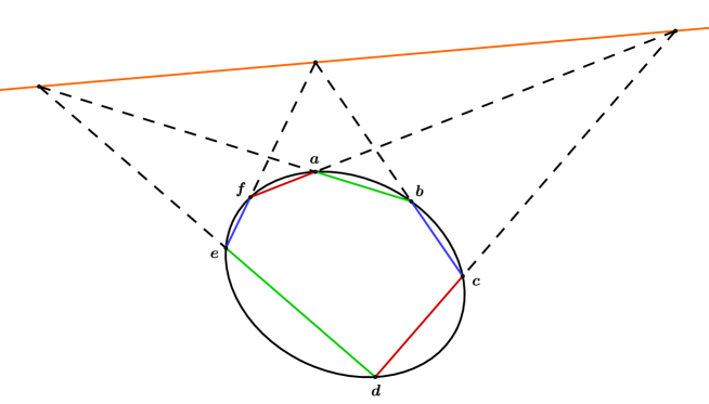
Diagram 1. The Pascal $L(abcdef)$

The line containing them is called the Pascal line (or just the Pascal) of the hexagon $abcdef$; we will denote it by $L(abcdef)$. If we shift the vertices cyclically or reverse their order, then the hexagon and its Pascal evidently do not change; hence there are $12$ distinct ways

$$L(abcdef)=L(bcdefa)=L(fedcba)\dots\text{etc}$$

of denoting the same Pascal. However, any essentially different arrangement of the vertices such as $L(acedbf)$ will a priori correspond to a different Pascal. A moment’s reflection will show that there are $6!/12=60$ such arrangements. Henceforth we will assume that the six points are in general position; in particular, this ensures that these sixty Pascals are pairwise distinct (see [7]).

2.2. Primal and dual notation

The notation $L(abcdef)$ for a Pascal line exhibits the particular hexagon from which it is defined. In [6], Christine Ladd extends this to a primal notation that gives natural names (indexed by combinations of the points $a,b,c,d,e$ and $f$) for all of the other nodes and lines in the multimysticum. The very similar notation used in [2] interprets the indices as permutations of the six points, with the understanding that inverse permutations index the same object. For example, the papers [2, 6] discuss a Steiner node $N(ace)(bdf)=N(eca)(fdb)$ that turns out to lie on the three Pascal lines $L(abcdef),L(adcfeb)$ and $L(afcbed)$ whose indexing permutations square to $ace.bdf$. The incidences between all nodes and lines in the multimysticum are described by convenient group theoretic relationships between indexing permutations, and in particular are invariant under the action of the group $S_{6}$ that permutes the six points.

In his construction of the multimysticum Veronese introduces linking lines and higher meeting points to pass between successive mutations. In [6], Ladd observes that there is no convenient primal notation for these linking objects. The solution turns out to be the use of a dual notation where we apply Sylvester’s outer automorphism of $S_{6}$ to the indexing permutations. The one downside to this notation is that it is now less obvious which hexagon leads to which Pascal line, but in compensation natural names become available for Veronese’s linking objects. Of course these natural names are no longer permutations, since otherwise their preimages under the outer automorphism would be natural primal names.

2.3. The dual notation

Define two sets

$$\textsc{ltr}=\{a,b,c,d,e,f\},\quad\textsc{num}=\{0,1,2,3,4,5\}.$$

consisting of six elements each. For any set $X$, let $S(X)$ denote the group of bijections $X\rightarrow X$. The following table defines an isomorphism $\zeta:S(\textsc{ltr})\longrightarrow S(\textsc{num})$, which is an outer automorphism. For instance, the entry in row $a$ and column $b$ is to be read as saying that $\zeta$ takes the $2$-cycle $a\,b$ to the element $2\,1\,.\,5\,3\,.\,0\,4$ of cycle type $2+2+2$.

$$\begin{array}[]{|c|c|c|c|c|c|c|}\hline\cr{}\hfil&b&c&d&e&f\\ \hline\cr a&21.53.04&24.51.03&20.54.13&25.01.34&23.50.14\\ b&{}\hfil&23.54.01&25.03.14&24.50.13&20.51.34\\ c&{}\hfil&{}\hfil&21.50.34&20.53.14&25.04.13\\ d&{}\hfil&{}\hfil&{}\hfil&23.51.04&24.53.01\\ e&{}\hfil&{}\hfil&{}\hfil&{}\hfil&21.54.03\\ \hline\cr\end{array}$$

Now, in order to find the dual notation for an arbitrary Pascal, say $L(acebfd)$, we find the image of the $6$-cycle $h=a\,c\,e\,b\,f\,d\in S(\textsc{ltr})$. Using the table, it is easy to calculate that

$$\zeta(h)=2\,.\,0\,4\,.\,1\,5\,3,\quad\text{and}\quad\zeta(h^{-1})=2\,.\,0\,4\,.\,1\,3\,5,$$

which are elements of cycle type $1+2+3$. In particular, the $1+2$ part of the image only depends on the set $\{h,h^{-1}\}$. Hence we relabel $L(acebfd)$ as $L{2}_{04}$ or $L{2}_{40}$. In this way, the sixty Pascals are labelled as $L{x}_{yz}$, where $x,y,z\in\textsc{num}$ are distinct elements and the order of $y,z$ is immaterial.

2.4.

The action of $\zeta^{-1}$ can be easily worked out from the same table. For instance, the pair $25$ appears in places $(a,e),(b,d)$ and $(c,f)$, from which we deduce that $2\,5\stackrel{{\scriptstyle\zeta^{-1}}}{{\longrightarrow}}a\,e\,.\,b\,d\,.\,c\,f$. In order to find the hexagon corresponding to an arbitrary Pascal, say $L{3}_{15}$, one calculates that

$$3\,.\,1\,5\,.\,0\,2\,4\stackrel{{\scriptstyle\zeta^{-1}}}{{\longrightarrow}}a\,d\,f\,c\,e\,b,$$

and hence $L{3}_{15}=L(adfceb)$. Of course, the hexagon is determined only up to a cyclic shift and reversal.

2.5.

There is an alternate way to see the labelling convention; which will be ‘generalised’ when we define the higher mutations in Section 3.

The Pascal $L{2}_{04}=L(acebfd)$ is the line passing through the intersection points $ac\cap bf,ce\cap df,ad\cap be$. We can introduce ‘dual notations’ for these points as follows: interpret the first as the element $a\,c\,.\,b\,f\in S(\textsc{ltr})$. When we apply $\zeta$, it gets sent to $2\,3\,.\,0\,4\in S(\textsc{num})$. The same calculation done on the other two points shows that $L{2}_{04}$ is the line passing through $21.04,23.04$ and $25.04$. The pattern for a general $L{x}_{yz}$ is now clear; it passes through $xu.yz,xv.yz,xw.yz$ where $\{u,v,w,x,y,z\}=\textsc{num}$.

Altogether there are $45$ such intersections points $xy.zw$, which will be called ordinary meeting points. Each of them lies on four Pascals; for instance, $12.35$ lies on $L{1}_{35},L{2}_{35},L{3}_{12}$ and $L{5}_{12}$. We will come across higher meeting points later in Section 3.1.

2.6.

We proceed to describe the rest of the elements in $\mathbb{H}$. The proofs of all the incidence theorems stated below may be found in [2, 3]. In keeping with the conventions of those papers, the points which participate in $\mathbb{H}$ will be called ‘nodes’. The notations for all the lines begin with $L$, and those for nodes begin with $N$. The construction sequence is as follows:

(5)

That is to say, the Kirkman nodes are constructed from Pascal lines using a concurrency theorem, the Plücker lines are constructed from Steiner nodes using a collinearity theorem, and so on.

2.7. The Kirkman nodes

A theorem of Kirkman shows that the Pascals $L{0}_{12},L{0}_{13},L{0}_{23}$ are concurrent. Their common point (called a Kirkman node or just a Kirkman) will be denoted by $N{0}_{45}$, where the pair $45$ is obtained by removing $0,1,2,3$ from num. It is understood that a parallel statement is true for any such indicial pattern; for example, the Pascals $L{1}_{02},L{1}_{05},L{1}_{25}$ are concurrent in the node $N{1}_{34}$ etc. Altogether, we have $60$ Kirkman nodes $N{x}_{yz}$.

Each Pascal contains three Kirkmans, and each Kirkman lies on three Pascals. The incidence pattern follows naturally from the notation. For instance, $L{1}_{23}$ contains the three Kirkmans $N{1}_{04},N{1}_{05},N{1}_{45}$. Similarly, $N{1}_{05}$ lies on $L{1}_{23},L{1}_{24},L{1}_{34}$. In particular, although the Pascals are logically prior, they can in fact be recovered from the Kirkmans. This dependence will look more symmetric when we come to the higher mutants in the next section.

The Pascals and the Kirkmans together form the mutable part $\mathbb{M}$ of $\mathbb{H}$. The fixed part $\mathbb{F}$ is made of two more kinds of lines and nodes which are described below.

2.8. Steiner nodes and Cayley lines

Choose three elements in num, say $0,2,5$. There are three Pascal lines, namely $L{1}_{34},L{3}_{14},L{4}_{13}$, whose labels avoid these three elements. A theorem of Steiner shows that these three Pascals are concurrent. Their common point is the Steiner node $N025$.

An analogous statement is true of the Kirkman nodes; that is to say, $N{1}_{34},N{3}_{14},N{4}_{13}$ are collinear; they lie on the Cayley line $L025$. Thus, there are $\binom{6}{3}=20$ lines and points respectively labelled $Lxyz$ and $Nxyz$, where $x,y,z\in\textsc{num}$ are distinct elements whose order is immaterial.

The Steiner node $Nxyz$ lies on the Cayley line $Luvw$, whenever $\{x,y,z,u,v,w\}=\textsc{num}$. For instance, $N024$ lies on $L135$.

2.9. Plücker lines and Salmon nodes

Choose two elements in num, say $2$ and $4$. This leaves out $0,1,3,5$. Now consider all Steiner nodes formed using these four leftover numbers, namely $N013,N015,N035$ and $N135$. A theorem of Plücker shows these four lie on a line, which we call the Plücker line $L24$.

An analogous statement is true of the Cayley lines; that is to say, $L013,L015,L035$ and $L135$ are concurrent in a point which will be called the Salmon node $N24$. There are $\binom{6}{2}=15$ such lines and points respectively labelled $Lxy$ and $Nxy$, where $x,y\in\textsc{num}$ are distinct elements whose order is immaterial.

This completes the description of $\mathbb{H}$, with its $60+20+15=95$ lines and 95 points. To recapitulate, all the Pascal lines and Kirkman nodes $L{x}_{yz},N{x}_{yz}$ are in the mutable part $\mathbb{M}$, whereas all the lines and nodes defined in Sections 2.8–2.9 are in the fixed part $\mathbb{F}$. For a general choice of six points on the conic, there are no incidences apart from those already mentioned.

2.10.

The articles by Conway and Ryba [2, 3] contain all of the preceding material in a rather concentrated form. One of the best early surveys of the field is due to George Salmon (see [10, Notes]). Much of this material is also explained by H. F. Baker in his note ‘On the Hexagrammum Mysticum of Pascal’ in [1, Note II]. Although his labelling scheme is ostensibly different from the one used here; it is based upon the same foundational notion, namely the outer automorphism of $S_{6}$. Several more older sources are listed in the bibliographies of [2, 3]. Many of the combinatorial and geometric aspects of the outer automorphism are discussed in [5].

Broadly speaking, there are (at least) two entirely different methods available for proving all of these incidences. One is to use Desargues’ theorem repeatedly, as in [2] or in the ‘Notes’ by Salmon [10]. Another approach, which can be attributed to Cremona and Richmond, is to use the geometry of lines on a nodal cubic surface (see [8, 9]).

The Steiner-Cayley elements have incidence relations with the Pascal-Kirkman as well as Plücker-Salmon elements. However, there are no direct incidence relations going across the latter two; that is to say, none of the Plücker lines contains any of the Kirkman nodes and none of the Salmon nodes lies on any of the Pascal lines.

Therefore, the Steiner-Cayley elements are in some ways central to the structure of $\mathbb{H}$. They will naturally serve as bases for the two ranges described below.

2.11. The Kirkman range

Consider an arbitrary Kirkman node, say $N{3}_{05}$. It lies on the Cayley line $L124$, which also contains the nodes $N05$ and $N305$. Thus we have three points

$$N05,\quad N305,\quad N{3}_{05},$$

on $L124$ which, in effect, create a coordinate system on this line. In other words, there is a unique isomorphism $f:L124\longrightarrow{\mathbb{P}}^{1}$ such that these points are taken to $\infty,0,1$ respectively. Then each point $Q\in L124$ is uniquely identified by its image $f(Q)\in{\mathbb{P}}^{1}$.

In the next section we will see that the Kirkman point $N{3}_{05}=N{3}_{05}^{(0)}$ has higher mutants $N{3}_{05}^{(i)}$ for $i\geqslant 1$, all of which lie on $L124$. Hence we have a range

$$N05,\quad N305,\quad N{3}_{05},\quad N{3}_{05}^{(1)},\quad N{3}_{05}^{(2)},\dots$$

on $L124$. In general, given a Kirkman point $N{x}_{yz}$, write $\{x,y,z,u,v,w\}=\textsc{num}$, and consider the range

$$Nyz,\quad Nxyz,\quad N{x}_{yz},\quad N{x}_{yz}^{(1)},\quad N{x}_{yz}^{(2)},\dots$$ (6)

on the Cayley line $Luvw$. Let $f:Luvw\longrightarrow{\mathbb{P}}^{1}$ denote the isomorphism which takes the first three points to $\infty,0,1$ respectively. Now the first part of our main theorem is as follows:

Theorem 2.1 (First Part).

With notation as above, the range (6) is isomorphic to the Veronese sequence given in (4). In other words, we have $f(N{x}_{yz}^{(i)})=\alpha_{i}$ for $i\geqslant 1$.

In particular, as an abstract projective range, the sequence of nodes in (6) is independent of the indices $x,y,z$, and also of the initial choice of the sextuple on the conic. One can see this schematically in Diagram 2. The blue nodes $N^{(2r+1)}$ at odd heights have a limiting position (shown as a red cross), while the green nodes $N^{(2r)}$ at even heights have a different limiting position (shown as a pink cross).

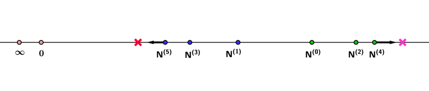
Diagram 2. The Kirkman range

There are a few variants of this theorem to be described below; a combined proof for all of them will be given in Section 4.

2.12. The Pascal range

Instead of a Kirkman node, one can begin with a Pascal line and carry out exactly the same construction with the roles of $N$ and $L$ interchanged. Thus, just as in (6), we have a sequence of lines

$$Lxyz,\quad Lyz,\quad Lx_{yz},\quad L{x}_{yz}^{(1)},\quad L{x}_{yz}^{(2)},\dots$$ (7)

all passing through the Steiner node $Nuvw$.

Notice that the ranges in (6) and (7) formally look the same from the third element onwards (with $N$ and $L$ interchanged), but the first two elements have been transposed. The Kirkman range starts as $Nyz,Nxyz$, whereas the Pascal range starts as $Lxyz,Lyz$. This is, of course, deliberate.

Theorem 2.2 (Second Part).

With notation as above, the range (7) is also isomorphic to the Veronese sequence.

The corresponding schema is shown in Diagram 3. The Pascals at the odd heights (shown in blue) converge to the red line, whereas those at the even heights (shown in green) converge to the pink line.

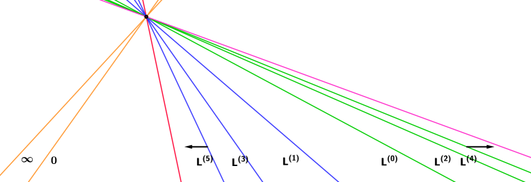
Diagram 3. The Pascal range

Either of the ranges above picks up one geometric element from each of the $\mathbb{M}^{(i)}$. By contrast, there are two more infinite sequences, namely the ‘meeting range’ and the ‘linking range’, which are associated to the mutations $\mathbb{M}^{(i)}\longrightarrow\mathbb{M}^{(i+1)}$. As such, their elements could be said to lie ‘midway’ between two adjacent $\mathbb{M}^{(i)}$. They will also turn out to be isomorphic to the Veronese sequence.

3. Veronese mutations and the Multimysticum

In this section, we will describe the process of mutation and in particular the two new ranges. Once this set-up is in place, the proof of the main theorem itself will be rather concise. Nearly all the material in this section may be found in Veronese’s original memoir [11], and also in the subsequent paper by Ladd [6].

Let $i$ be an index $\geqslant 0$. If $i$ is even, then the passage from $\mathbb{M}^{(i)}$ to $\mathbb{M}^{(i+1)}$ uses an auxiliary system of ‘linking lines’; whereas for $i$ odd, it uses a system of ‘meeting points’. Recall that $\mathbb{M}^{(0)}$ represent the usual Pascal lines and Kirkman nodes. The higher ‘Pascals’ and ‘Kirkmans’ lie in $\mathbb{M}^{(i)}$ for $i\geqslant 1$, but it should be kept in mind that they do not come from an actual sextuple of points on a conic.

Along the way, we will refer to several incidence properties of the new points and lines as they arise. The proofs of all of these may be found in [3].

3.1.

Assume that $i$ is even. The mutation $\mathbb{M}^{(i)}\longrightarrow\mathbb{M}^{(i+1)}$ can be schematically represented as follows:

(8)

To wit, the Kirkmans at height $i$ are used to create a system of linking lines, which are in turn used to construct Kirkmans at height $i+1$. These new nodes are then used to construct new Pascals at height $i+1$. The Pascals at height $i$ play no direct role in the construction. The recipe is as follows:

1. For any four elements in num, say $1,2,3,4$, define the linking line

   $$1^{(i+1)}\,2^{(i+1)}.\,3^{(i)}\,4^{(i)}=\text{line joining the nodes $N{3}_{12}^{(i)}$ and $N{4}_{12}^{(i)}$.}$$ (9)

   There are $\binom{6}{4}\binom{4}{2}=90$ such lines.

2. Now define a higher Kirkman node, say $N{1}_{34}^{(i+1)}$, as the common point of the lines

   $$1^{(i+1)}\,x^{(i+1)}.\,3^{(i)}\,4^{(i)},\quad x=0,2,5.$$

   It is a fact that these three lines are concurrent, and hence this node is well-defined (see [3]).

3. Once all the new Kirkmans are in place, the new Pascals are constructed from them as in Section  2.7. That is to say, define $L{1}_{23}^{(i+1)}$ as the line containing

   $$N{1}_{04}^{(i+1)},\quad N{1}_{05}^{(i+1)},\quad N{1}_{45}^{(i+1)}.$$

   Again, it is a fact that these three new nodes are collinear, and hence the new Pascal is well-defined.

The first two steps are illustrated in Diagram 4. The Kirkmans at height $i$ (shown in blue) are connected by linking lines (shown in green). Three of these lines are concurrent in the new Kirkman (shown in red) at height $i+1$.

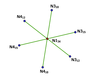
Diagram 4. For $i$ even, the blue Kirkmans at height $i$ lead to the red Kirkman at height $i+1$.

3.2.

Now assume that $i$ is odd. The mutation $\mathbb{M}^{(i)}\longrightarrow\mathbb{M}^{(i+1)}$ is given by a ‘reciprocal’ procedure. Schematically, we have:

(10)

The Pascals at height $i$ are used to create a system of meeting points, which are in turn used to construct Pascals at height $i+1$. These new lines are then used to construct new Kirkmans at height $i+1$. The Kirkmans at height $i$ play no direct role in the construction. The recipe, which follows by making cosmetic changes to the earlier recipe, is as follows:

1. For any four elements in num, say $1,2,3,4$, construct the higher meeting point

   $$1^{(i+1)}\,2^{(i+1)}.\,3^{(i)}\,4^{(i)}=\text{point of intersection of the lines $L{3}_{12}^{(i)}$ and $L{4}_{12}^{(i)}$.}$$ (11)

   There are $90$ such points. They are notationally distinguished from the ordinary meeting points in Section 2.5, and hence we will omit the adjective ‘higher’ if no confusion is likely.

2. Now define a higher Pascal, say $L{1}_{34}^{(i+1)}$, as the line passing through the meeting points

   $$1^{(i+1)}\,x^{(i+1)}.\,3^{(i)}\,4^{(i)},\quad x=0,2,5.$$

   These three points are in fact collinear, hence the Pascal is well-defined.

3. Once the new Pascals are in place, the new Kirkmans are constructed from them as in Section  2.7. That is to say, define $N{1}_{23}^{(i+1)}$ as the common point of the concurrent lines

   $$L{1}_{04}^{(i+1)},\quad L{1}_{05}^{(i+1)},\quad L{1}_{45}^{(i+1)}.$$

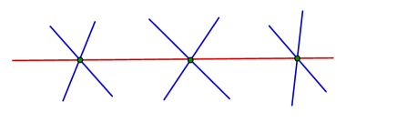
Diagram 5. For $i$ odd, the blue Pascals at height $i$ lead to the red Pascal at height $i+1$.

The first two steps are shown in Diagram 5. The Pascals at height $i$ (shown in blue) intersect in meeting points (shown in green). Three of the meeting points are collinear in the new Pascal (shown in red) at height $i+1$. We have omitted all the labels, since they can be obtained from Diagram 4 by replacing each $N$ with an $L$.

This completes the process of defining the mutations. It is a fact that all the new Kirkmans and Pascals have exactly the same incidence relations with the Cayley lines and Steiner nodes respectively. For instance, the Kirkman $N{1}_{34}^{(i)}$ lies on the Cayley line $L025$ for all values of $i\geqslant 0$. Similarly, the Pascal $L{1}_{34}^{(i)}$ passes through the Steiner node $N025$ for all values of $i\geqslant 0$. This ensures that the Kirkman range in Section 2.11, and the Pascal range in Section 2.12 are well-defined.

3.3.

Notice that the linking lines in (9) and meeting points in (11) have formally the same notation. It is the parity of $i$ which tells them apart. Moreover, the symmetry $xy.zw=zw.xy$ which holds for ordinary meeting points in Section 2.5 is no longer valid for higher meeting points and linking lines; that is to say,

$$1^{(i+1)}\,2^{(i+1)}.\,3^{(i)}\,4^{(i)}\neq 3^{(i+1)}\,4^{(i+1)}.\,1^{(i)}\,2^{(i)}.$$

Thus there are $90$ higher meeting points for each odd $i$ and $90$ linking lines for each even $i$, but only $45$ ordinary meeting points.

The larger number of higher meeting points proves that no set of $60$ higher Pascal lines can arise as the Pascal lines corresponding to six points on any conic. (Otherwise, the $45$ meeting points corresponding to these Pascal lines would have to match the $90$ higher meeting points obtained as intersections of higher Pascal lines. This is clearly impossible since $45\neq 90$.) A similar argument shows that no set of Kirkman nodes (or higher Kirkman nodes) can arise as the $60$ points obtained by applying Brianchon’s theorem to a set of six tangents to a conic.

We now define the Veronese nodes and Ladd lines. All the incidences referred to are proved in [3].

3.4. The Ladd lines

Assume $i$ to be odd, and consider the two meeting points

$$1^{(i+1)}\,2^{(i+1)}.\,3^{(i)}\,4^{(i)}\quad\text{and}\quad 3^{(i+1)}\,4^{(i+1)}.\,1^{(i)}\,2^{(i)}.$$

It is a remarkable fact that the line joining them is independent of $i$. It is called the Ladd line $L12.34$. There are $45$ such lines $Lxy.zw$.

The Ladd line $L12.34$ contains the Salmon node $N05$ and the ordinary meeting point $12.34$. Define the Plücker-Ladd node $N{1}{2}.{3}^{\prime}{4}^{\prime}$ to be the intersection of the Plücker line $L34$ and the Ladd line $L12.34$. At this point, we have all the ingredients necessary to create a range on $L12.34$. Write

$$p_{i}=3^{(i+1)}\,4^{(i+1)}.\,1^{(i)}\,2^{(i)}\quad\text{and}\quad q_{i}=1^{(i+1)}\,2^{(i+1)}.\,3^{(i)}\,4^{(i)},$$

and consider the range

$$N05,\quad N{1}{2}.{3}^{\prime}{4}^{\prime},\quad 12.34,\quad p_{1},\quad q_{1},\quad p_{3},\quad q_{3},\quad p_{5},\quad q_{5},\dots$$ (12)

which will be called the ‘meeting range’, since after the initial stretch of two points it is entirely made of meeting points. Notice that there are $90$ such ranges, although there are only $45$ Ladd lines. This is so because $N{1}{2}.{3}^{\prime}{4}^{\prime}$ and $N{3}{4}.{1}^{\prime}{2}^{\prime}$ are distinct points belonging to distinct ranges on the same line. This circumstance will prove useful in the proof of the main theorem (see Section 4.4 below).

3.5. The Veronese nodes

Assume $i$ to be even, and consider the two linking lines

$$1^{(i+1)}\,2^{(i+1)}.\,3^{(i)}\,4^{(i)}\quad\text{and}\quad 3^{(i+1)}\,4^{(i+1)}.\,1^{(i)}\,2^{(i)}.$$

Their point of intersection is independent of $i$. It is called the Veronese node $N12.34$. There are $45$ such nodes $Nxy.zw$.

The Plücker line $L05$ passes through the Veronese node $N12.34$. Define the Salmon-Veronese line $L{1}{2}.{3}^{\prime}{4}^{\prime}$ to be the line joining the Salmon node $N34$ and the Veronese node $N12.34$. Now write

$$r_{i}=3^{(i+1)}\,4^{(i+1)}.\,1^{(i)}\,2^{(i)}\quad\text{and}\quad s_{i}=1^{(i+1)}\,2^{(i+1)}.\,3^{(i)}\,4^{(i)},$$

and consider the range of lines

$$L{1}{2}.{3}^{\prime}{4}^{\prime},\quad L05,\quad r_{0},\quad s_{0},\quad r_{2},\quad s_{2},\quad r_{4},\quad s_{4},\dots$$ (13)

all passing through $N12.34$. In analogy with the above, this will be called a ‘linking range’. There are $90$ such ranges with two of them based upon each Veronese node.

The constructions in (12) and (13) are not perfectly parallel. Apart from the transposition in the first two elements, there is an additional asymmetry which comes from the fact that there is no linking line on an equal footing with the meeting point $12.34$.

Theorem 3.1 (Third Part).

With notation as above, the ranges in (12) and (13) are also isomorphic to the Veronese sequence.

Thus, we have altogether $60+90=150$ point ranges, and the same number of line ranges, all isomorphic to the Veronese sequence. Although we did not initially say so, the Ladd lines and Veronese nodes can also been seen as belonging to the fixed part $\mathbb{F}$.

4. Proof of the Main Theorem

4.1.

In this section, we will finally prove the main theorem. It will be convenient to label the four ranges. Write $\{u,v,w,x,y,z\}=\textsc{num}$, and let

$${\mathbb{K}}[x,yz] =\text{Kirkman range in~{}(\ref{kirkman.range}) based upon the Cayley line $Luvw$,}$$ (14)

$${\mathbb{P}}[x,yz] =\text{Pascal range in~{}(\ref{pascal.range}) based upon the Steiner node $Nuvw$,}$$

$${\mathbb{M}}[xy.z^{\prime}w^{\prime}] =\text{Meeting range in~{}(\ref{meeting.range}) based upon the Ladd line $Lxy.zw$,}$$

$$\Lambda[xy.z^{\prime}w^{\prime}] =\text{Linking range in~{}(\ref{linking.range}) based upon the Veronese node $Nxy.zw$.}$$

Recall that we get altogether $150$ point ranges and the same number of line ranges by assigning the letters $u,v,\dots,z$ to $0,1,\dots,5$ in all possible ways.

Now the main theorem will proved in the following steps:

1. First, we show that all the $300$ ranges in (14) are isomorphic to each other. This implies that any of them is isomorphic to a range

   $$\infty,\quad 0,\quad\beta_{0}=1,\quad\beta_{1},\quad\beta_{2},\quad\beta_{3},\dots$$ (15)

   on ${\mathbb{P}}^{1}$ for some as yet unknown complex numbers $\beta_{i}$.

2. Next, we show that:

   • For $i$ odd, we have $\beta_{i}+\beta_{i+1}=2$.

   • As $m$ ranges over the nonnegative integers, the sum $1/\beta_{2m}+1/\beta_{2m+1}$ remains independent of $m$.

3. Finally, we show that $\beta_{1}=1/2$, and hence this sum is in fact $3$. This shows that (15) is identical to the Veronese sequence in (4), which completes the argument.

4.2. Aligned ranges

Let $Q$ and $E$ be respectively a point and a line in the projective plane, such that $Q\notin E$. Assume that $(q_{1},q_{2},\dots)$ and $(e_{1},e_{2},\dots)$ are ranges based upon $Q$ and $E$ respectively; that is to say, $q_{i}$ are lines through $Q$ and $e_{i}$ are points on $E$. If $e_{i}$ is incident with $q_{i}$ for all $i$, then the ranges are said to be aligned (see Diagram 6). In particular, they are then isomorphic. We will complete step one by using this technique repeatedly.

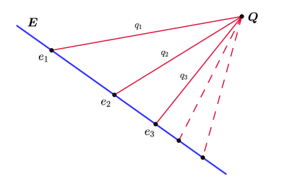
Diagram 6. Aligned (and hence isomorphic) ranges

Many of the proofs below depend upon exploiting a specific indicial pattern. In such cases, for the sake of vividness, we will use specific numbers from $0$ through $5$ instead of letters $u,v,\dots,z$. This should make the proofs easier to follow. We will use the incidence properties of points and lines from Sections 2.7–2.9, and also those involving higher mutants from Sections 3.1–3.2.

4.3.

Notice that the Kirkman $N{2}_{04}$ lies on the Pascal $L{2}_{15}$. This incidence lifts to an alignment between the corresponding Kirkman and Pascal ranges: ${\mathbb{K}}[2,04]$ and ${\mathbb{P}}[2,15]$. Indeed, the two ranges respectively correspond to the two rows:

$$\begin{array}[]{|c|c|c|c|c}\hline\cr N04&N204&N{2}_{04}&N{2}_{04}^{(1)}&\dots\\ \hline\cr L215&L15&L{2}_{15}&L{2}_{15}^{(2)}&\dots\\ \hline\cr\end{array}$$

Now it is merely a matter of checking that the node and the line in any column are incident. For instance, the node $N204$ in the second column is incident with the line $L15$ below it, because $0,2,4$ are disjoint from $1,5$. In summary, if we take $Q=N034$ (the base of the Pascal range), $E=L125$ (the base of the Kirkman range) and think of the rows as $(e_{1},e_{2},\dots),(q_{1},q_{2},\dots)$ respectively, then everything matches Diagram 6.

This observation, used repeatedly, will allow us to correlate a large number of ranges.

Lemma 4.1.

Fix an element $x\in\textsc{num}$. Then all Kirkman ranges ${\mathbb{K}}[x,\bullet\bullet]$ and Pascal ranges ${\mathbb{P}}[x,\bullet\bullet]$ are isomorphic.

In either instance, the bullets stand for any two indices different from $x$.

Proof.  Consider the following chain of alternating Pascals and Kirkmans:

$$L{0}_{12},\quad N{0}_{34},\quad L{0}_{51},\quad N{0}_{23},\quad L{0}_{45}.$$

It has the property that any adjacent node-line pair is incident; in fact the chain is constructed by keeping $x=0$ fixed, and going through the sequence $1-2-3-4-5-1$ cyclically in disjoint pairs. Hence, the corresponding ranges

$${\mathbb{P}}[0,12],\quad{\mathbb{K}}[0,34],\quad{\mathbb{P}}[0,51],\quad{\mathbb{K}}[0,23],\quad{\mathbb{P}}[0,45],$$

are isomorphic. Now observe that this captures all possible indicial patterns. For instance, two Pascal ranges ${\mathbb{P}}[x,\bullet\bullet]$ must either look like ${\mathbb{P}}[0,12]$ and ${\mathbb{P}}[0,51]$ with one overlap in the remaining indices, or like ${\mathbb{P}}[0,12]$ and ${\mathbb{P}}[0,45]$ with no such overlap. We have shown they are isomorphic in either case. Hence all Kirkman ranges ${\mathbb{K}}[0,\bullet\bullet]$ are isomorphic to this common Pascal range, and also to each other. ∎

We can picture the Pascal and Kirkman ranges (altogether $60$ and $60$) as being distributed across six islands, corresponding to the values $x=0,1,\dots,5$. By the lemma above, we know that the ranges on each island ($10$ and $10$) are isomorphic amongst themselves. The meeting and linking ranges will allow us to pass from one island to another.

Lemma 4.2.

Let $x,y,z,w\in\textsc{num}$. Then

1. the Kirkman range ${\mathbb{K}}[x,yz]$ is aligned with the linking range $\Lambda[xw.y^{\prime}z^{\prime}]$; and

2. the Pascal range ${\mathbb{P}}[x,yz]$ is aligned with the meeting range ${\mathbb{M}}[xw.y^{\prime}z^{\prime}]$.

Proof.  The argument is very similar to the one in Section 4.3, and merely amounts to checking that the corresponding lines and points are incident. We will give an illustration for (1). Let $x,y,z,w=1,3,4,2$ respectively. Then the fifth node in ${\mathbb{K}}[1,34]$ and the fifth line in $\Lambda[12.3^{\prime}4^{\prime}]$ are respectively

$$N{1}_{34}^{(2)}\quad\text{and}\quad 3^{(3)}4^{(3)}.1^{(2)}2^{(2)},$$

which are incident by the very definition of the linking line. The remaining verifications are equally routine, and we leave them to the reader. ∎

One can now pass from one island to another.

Lemma 4.3.

Let $x,y,z,w\in\textsc{num}$. Then

1. the Kirkman ranges ${\mathbb{K}}[x,yz]$ and ${\mathbb{K}}[w,yz]$ are isomorphic, and

2. the Pascal ranges ${\mathbb{P}}[x,yz]$ and ${\mathbb{P}}[w,yz]$ are isomorphic.

Proof.  The two Kirkman ranges are isomorphic because each is aligned with $\Lambda[xw.y^{\prime}z^{\prime}]$. The argument for Pascal ranges is essentially the same. ∎

The preceding lemmas culminate in the following proposition, which completes step one in the proof of the main theorem.

Proposition 4.4.

All the $300$ ranges in (14) are isomorphic to each other. ∎

4.4.

Each of the expressions involved in step two involves two adjacent values of $\beta_{i}$. The trick is to use an involution (i.e., an automorphism of order $2$) which will interchange $p_{i}$ with $q_{i}$ in the meeting range, and similarly $r_{i}$ with $s_{i}$ in the linking range.

Recall that each automorphism of ${\mathbb{P}}^{1}$ is given by a fractional linear transformation

$${\mathbb{P}}^{1}\stackrel{{\scriptstyle f}}{{\longrightarrow}}{\mathbb{P}}^{1},\qquad f(z)=\frac{pz+q}{rz+s}.$$

The matrix $\left[\begin{array}[]{cc}p&q\\ r&s\end{array}\right]$ is nonsingular, and determined up to a nonzero scalar.

Proposition 4.5.

We have $\beta_{i}+\beta_{i+1}=2$ for all odd values of $i$.

Proof.  Consider the isomorphic ranges ${\mathbb{M}}[12.3^{\prime}4^{\prime}]$ and ${\mathbb{M}}[34.1^{\prime}2^{\prime}]$, both of which are based upon the Ladd line $L12.34$. They are respectively shown in the rows below:

$$\begin{array}[]{|c|c|c|c|c|c|c|c|}\hline\cr N05&N12.3^{\prime}4^{\prime}&12.34&p_{1}&q_{1}&p_{2}&q_{2}&\dots\\ \hline\cr N05&N34.1^{\prime}2^{\prime}&34.12&q_{1}&p_{1}&q_{2}&p_{2}&\dots\\ \hline\cr\end{array}$$

Observe that the first and the third nodes coincide, and fourth onwards they get interchanged in pairs. Now fix coordinates on $L12.34$ such that the top row gets identified with the sequence (15). Then the rows appear as

$$\begin{array}[]{|c|c|c|c|c|c|c|c|}\hline\cr\infty&0&1&\beta_{1}&\beta_{2}&\beta_{3}&\beta_{4}&\dots\\ \hline\cr\infty&\mu&1&\beta_{2}&\beta_{1}&\beta_{4}&\beta_{3}&\dots\\ \hline\cr\end{array}$$

for some constant $\mu$. Hence there exists a fractional linear transformation $f(z)=\frac{pz+q}{rz+s}$ which takes the first row to the second. Now $f(\infty)=\infty$ implies that $r=0$, and we may assume $s=1$. Then $f(1)=1$ implies that $f(z)=pz+(1-p)$ for some $p$. Since $f(f(z))=z$ and $f$ is not the identity, we must have $p=-1$, i.e., $f(z)=2-z$. Hence it follows that $\beta_{i+1}=f(\beta_{i})=2-\beta_{i}$ for all odd values of $i$. ∎

Now we use a similar argument on the linking range.

Proposition 4.6.

As $m$ ranges over the nonnegative integers, the sum $1/\beta_{2m}+1/\beta_{2m+1}$ remains independent of $m$.

Proof.  Consider the isomorphic ranges $\Lambda[12.3^{\prime}4^{\prime}]$ and $\Lambda[34.1^{\prime}2^{\prime}]$, both of which are based upon the Veronese node $N12.34$. They are respectively shown in the rows below:

$$\begin{array}[]{|c|c|c|c|c|c|c|}\hline\cr L12.3^{\prime}4^{\prime}&L05&r_{0}&s_{0}&r_{2}&s_{2}&\dots\\ \hline\cr L34.1^{\prime}2^{\prime}&L05&s_{0}&r_{0}&s_{2}&r_{2}&\dots\\ \hline\cr\end{array}$$

The second entry is the same in both ranges, and from the third onwards they get interchanged in pairs. Now fix coordinates on the planar pencil of lines through $N12.34$ so that the top row is identified with the sequence (15). Then the rows appear as

$$\begin{array}[]{|c|c|c|c|c|c|c|}\hline\cr\infty&0&1&\beta_{1}&\beta_{2}&\beta_{3}&\dots\\ \hline\cr\mu&0&\beta_{1}&1&\beta_{3}&\beta_{2}&\dots\\ \hline\cr\end{array}$$

for some constant $\mu$. As above, there must exists a fractional linear transformation $f(z)=\frac{pz+q}{rz+s}$ which takes the first row to the second. Now $f(0)=0$ implies that $q=0$ and we may assume $p=1$. Since $f$ is a non-identity function such that $f(f(z))=z$, we must have $s=-1$ and hence $f(z)=z/(rz-1)$ for some $r$. Now $f(\beta_{2})=\beta_{3}$ implies that $r=1/\beta_{2}+1/\beta_{3}$. The same argument applies to all such pairs, and thus we get

$$r=1+\frac{1}{\beta_{1}}=\frac{1}{\beta_{2}}+\frac{1}{\beta_{3}}=\frac{1}{\beta_{4}}+\frac{1}{\beta_{5}}=\dots$$

∎

4.5.

It only remains to find $\beta_{1}$. Since the anticipated answer is $1/2$, the reader may have already guessed that harmonicity is implicated. Consider the first four elements in each of the Kirkman ranges ${\mathbb{K}}[0,23]$ and ${\mathbb{K}}[1,23]$, namely

$$N23,\quad N023,\quad N{0}_{23},\quad N{0}_{23}^{(1)}\qquad\text{and}\qquad N23,\quad N123,\quad N{1}_{23},\quad N{1}_{23}^{(1)}.$$ (16)

We may identify both of them with the range $(\infty,0,1,\beta_{1})$. We will construct a nontrivial automorphism of this quadruple. Join the four nodes of the first quadruple to the (ordinary) meeting point $01.45$. This creates the line quadruple:

$$L01.45,\quad L{1}_{45},\quad L{0}_{45},\quad 0^{(1)}1^{(1)}.\,2^{(0)}3^{(0)}$$ (17)

(for the last incidence, see the last line on ‘Elevation’ on page 48 of [3]).

Now observe that if we now join the second quadruple in (16) to the same meeting point, then the middle two elements in (17) get interchanged and those at either end remain unchanged. It follows that $(\infty,0,1,\beta_{1})$ is isomorphic to $(\infty,1,0,\beta_{1})$; that is to say, this is a harmonic quadruple. The only possible linear fractional transformation which takes the first to the second is $f(z)=1-z$. Hence $f(\beta_{1})=1-\beta_{1}=\beta_{1}$, which forces $\beta_{1}=1/2$. This completes the proof of the main theorem. ∎

4.6.

Although our theorem shows that many of the infinite ranges that belong to the multimysticum are absolutely invariant, this is certainly not the case for all ranges within the system. For example, the Kirkman ranges ${\mathbb{K}}[0,12],{\mathbb{K}}[1,02],{\mathbb{K}}[2,01]$ all lie on the Cayley line $L345$, but there is no fixed set of projective coordinates for the union of these ranges. Moreover, there are other points on this Cayley line such as the anti-Kirkman nodes ${\rm{{{\rm a}{N}}}}0_{12}$, ${\rm{{{\rm a}{N}}}}1_{02}$ and ${\rm{{{\rm a}{N}}}}2_{01}$ (see [3, p. 48]) which cannot be added to any of these ranges without sacrificing absolute invariance.

4.7.

The theorem opens up several new lines of inquiry. For instance, it is clear that some of the terms of the Veronese sequence become zero or undefined if the base field is of positive characteristic. It would be of great interest to study the structure of the multimysticum in such cases. We hope to pick up this thread in a possible sequel to this paper.

This paper is based upon a rather more compact version written jointly by the two authors with Professor John Conway. We should like to thank him for several helpful discussions.

Jaydeep Chipalkatti, Department of Mathematics, Machray Hall, University of Manitoba, Winnipeg, MB R3T 2N2, Canada
E-mail address: jaydeep.chipalkatti@umanitoba.ca

Alex Ryba, Department of Computer Science, Queens College, CUNY, 65-30 Kissena Boulevard, Flushing, NY 11367, USA
E-mail address: ryba@cs.qc.cuny.edu

–

References

- [1] H. F. Baker, Principles of Geometry, volume 2, University Press, Cambridge, 1922.
- [2] J. H. Conway and A. J. E. Ryba, The Pascal Mysticum Demystified. The Mathematical Intelligencer, 34, no. 3 (2012), 4–8.
- [3] J. H. Conway and A. J. E. Ryba, Extending the Pascal Mysticum. The Mathematical Intelligencer, 35, no. 2 (2013), 44–51.
- [4] H. S. M. Coxeter, The real projective plane, McGrawHill, New York, 1949.
- [5] B. Howard, J. Millson, A. Snowden, and R. Vakil, A description of the outer automorphism of , and the invariants of six points in projective space. J. Combin. Theory Ser. A, 115, no. 7 (2008), 1296–1303.
- [6] C. Ladd, The Pascal Hexagram, Amer. J. Math., 2 (1879), 1–12.
- [7] D. Pedoe, How many Pascal lines has a sixpoint? The Mathematical Gazette, , 25 (1941), 110–111.
- [8] H. W. Richmond, A symmetrical system of equations of the lines on a cubic surface which has a conical point. The Quarterly Journal of Pure and Applied Mathematics, 23 (1889), 170–179.
- [9] H. W. Richmond, The figure formed from six points in space of four dimensions. Math. Annalen, LIII (1869), 161–176.
- [10] G. Salmon, A Treatise on Conic Sections, Reprint of the 6th ed. by Chelsea Publishing Co., New York, 2005.
- [11] G. Veronese, Nuovi teoremi sull’Hexagrammum mysticum, Memorie della Reale Accademia dei Lincei, 3, no. 1 (1877), 649–703.