Estimating Monte Carlo variance from multiple Markov chains

Abstract

The ever-increasing power of the personal computer has led to easy parallel implementations of Markov chain Monte Carlo (MCMC). However, almost all work in estimating the variance of Monte Carlo averages, including the efficient batch means (BM) estimator, focuses on a single-chain MCMC run. We demonstrate that simply averaging covariance matrix estimators from multiple chains (average BM) can yield critical underestimates in small sample sizes, especially for slow mixing Markov chains. We propose a multivariate replicated batch means (RBM) estimator that utilizes information from parallel chains, thereby correcting for the underestimation. Under weak conditions on the mixing rate of the process, the RBM and ABM estimator are both strongly consistent and exhibit similar large-sample bias and variance. However, in small runs the RBM estimator can be dramatically superior. This is demonstrated through a variety of examples, including a two-variable Gibbs sampler for a bivariate Gaussian target distribution. Here, we obtain a closed-form expression for the asymptotic covariance matrix of the Monte Carlo estimator, a useful result for benchmarking in the future.

1 Introduction

Markov chain Monte Carlo (MCMC) algorithms have emerged as an essential tool for parameter estimation of target distributions when obtaining independent samples is inefficient. With increased computational power and the presence of multiple cores on personal computers, running parallel Markov chains dispersed over the state space is common for improved inference. On the other hand, output analysis in MCMC has predominantly focused on single-chain MCMC output with the understanding that multiple-chain analysis can follow from a simple averaging of information. We demonstrate that a simple averaging of the Monte Carlo limiting covariance matrix can yield significant underestimation, warranting specific methods for multiple-chain output analysis.

Let $F$ be the target distribution defined on a $d$-dimensional space $\mathcal{X}$, equipped with a countably generated $\sigma$-field. Let function $h:\mathcal{X}\to\mathbb{R}^{p}$ be such that $\mu=\int_{\mathcal{X}}h(x)F(dx)$ is a quantity of interest. Let $\{X_{1,t}\}_{t\geq 1},\dots,\{X_{m,t}\}_{t\geq 1}$ be $m$ independent $F$-ergodic Markov chains. The Monte Carlo estimator of $\mu$ from the $k$th Markov chain is

$$\hat{\mu}_{k}=\dfrac{1}{n}\displaystyle\sum_{t=1}^{n}h\left(X_{k,t}\right)\overset{a.s.}{\to}\mu\text{ as }n\to\infty\,,$$

where the convergence holds for any starting value. Consequently, the combined estimator of $\mu$ from the $m$ independent chains is $\hat{\mu}=m^{-1}\sum_{k=1}^{m}\hat{\mu}_{k}\,.$ If a Markov chain central limit theorem (CLT) holds, then irrespective of the starting value, there exists a $p\times p$ positive-definite matrix $\Sigma$ such that for all $k=1,\dots,m$, as $n\to\infty$,

$$\sqrt{n}(\hat{\mu}_{k}-\mu)\overset{d}{\to}N_{p}(0,\Sigma)\,.$$

Consequently, a CLT holds for $\hat{\mu}$ as well so that as $n\to\infty$,

$$\sqrt{mn}(\hat{\mu}-\mu)\overset{d}{\to}N_{p}(0,\Sigma)\,.$$ (1)

A significant goal in MCMC output analysis is estimating $\Sigma$ in order to ascertain the quality of estimation of $\mu$ via $\hat{\mu}$. This has a direct consequence on determining when to stop the MCMC sampler (Brooks and Gelman,, 1998; Flegal et al.,, 2008; Gelman and Rubin,, 1992; Gong and Flegal,, 2016; Roy,, 2019; Vats et al.,, 2019; Vehtari et al.,, 2020). Additionally, estimators of $\Sigma$ must be (strongly) consistent in order to yield nominal coverage for large termination sizes. Amongst the list of estimators, only the naive estimator of Brooks and Roberts, (1998), which estimates $\Sigma$ by the sample covariance matrix of $\hat{\mu}_{1},\dots,\hat{\mu}_{m}$, is specifically constructed for multiple-chains. We show that this estimator is not consistent and exhibits high variability when the number of parallel implementations is small.

Many estimators have been introduced for a single-chain implementation, including batch means (BM) estimators (Chen and Seila,, 1987), spectral variance estimators (Hannan,, 1970), regenerative estimators (Seila,, 1982), and initial sequence estimators (Dai and Jones,, 2017; Kosorok,, 2000). Vats et al., (2020) recommend the BM estimator due to its ease of implementation, universality of application, computational efficiency, and well established asymptotic properties.

Let $\hat{\Sigma}_{k}$ denote the BM estimator of $\Sigma$ from the $k$th chain. A default combined estimator of $\Sigma$, which we call the average batch means (ABM) estimator is, $\hat{\Sigma}=m^{-1}\sum_{k=1}^{m}\hat{\Sigma}_{k}\,.$ ABM naturally retains asymptotic properties of $\hat{\Sigma}_{k}$, since the $m$ chains are independent. This averaging of the variance is reasonable for independent and identically distributed samples. However, before each chain has adequately explored the state space, chains may dominate different parts of $\mathcal{X}$, so that each $\hat{\Sigma}_{k}$ significantly underestimates the truth. As a result, the ABM estimator also underestimates the truth and many of the benefits of running parallel chains from dispersed starting values are lost.

In the steady-state literature for univariate $\phi$-mixing processes ($p=1$), Argon and Andradóttir, (2006) introduced a replicated batch means (RBM) estimator that estimates $\Sigma$ by essentially centering the chain around the overall mean $\hat{\mu}$, instead of the $k$th chain mean, $\hat{\mu}_{k}$. We develop the RBM estimator in this multivariate setting and obtain (strong) consistency, large-sample bias and variance results for the larger class of $\alpha$-mixing processes. Since deviation is measured from the global mean, in the event that chains explore different parts of the state space, RBM estimates yield dramatic improvements over ABM.

Asymptotically, RBM and ABM are no different, but RBM has clear advantages over ABM in finite samples which we illustrate through three examples: a Gibbs sampler for a bivariate Gaussian target, a Metropolis-Hastings sampler for the tricky Rosenbrock distribution, and a Metropolis-Hastings sampler for a Bayesian multinomial regression posterior. For the Gaussian Gibbs sampler, we obtain the true value of $\Sigma$. In the past, the true $\Sigma$ has only been known for some time-series processes, but never for a more traditional MCMC problem. Obtaining the true $\Sigma$ allows for this example to be used for benchmarking the performance of new estimators in the future. Over all three examples, the results are consistent: the RBM estimator is at least as good as the ABM estimator with no additional computation costs. However, when dealing with slow mixing Markov chains or small sample sizes, RBM can far outperform ABM, yielding a significantly more reliable estimator of $\Sigma$.

2 Background and assumptions

Much of our focus is on MCMC, but our results apply more generally to $\alpha$-mixing processes. Our first assumption is on the mixing rate of $\{X_{k,t}\}$ and the moments of $\{Y_{k,t}\}=\{h(X_{k,t})\}$.

Assumption 1.

For some $\delta>0$, $\text{E}_{F}\|Y_{k,1}\|^{2+\delta}<\infty$ and there exists $\epsilon>0$ such that $\{X_{k,t}\}$ is $\alpha$-mixing with $\alpha(n)=o\left(n^{-\left(2+\epsilon\right)\left(1+2/\delta\right)}\right)$ for all $k=1,\dots,m$.

Assumption 1 will be our umbrella assumption on the process, however, we bring special focus to when this assumption is satisfied by Markov chains. Let $P:\mathcal{X}\times\mathcal{B}(\mathcal{X})\to[0,1]$ be an $F$-invariant Markov chain transition kernel, where for $x\in\mathcal{X}$ and $A\in\mathcal{B}(\mathcal{X})$, $P(x,A)=\Pr(X_{2}\in A|X_{1}=x)$. The $n$-step transition is $P^{n}(x,A)=\Pr(X_{n+1}\in A\mid X_{1}=x)$. We assume that $P$ is Harris ergodic, which guarantees ergodicity and implies that the Markov chain is $\alpha$-mixing (Jones,, 2004). Assumption 1 may hold when the Markov chain is polynomially ergodic. That is, suppose there exists $M:\mathcal{X}\to[0,\infty)$ with $\text{E}_{F}M<\infty$ and $\xi>0$ such that

$$\|P^{n}(x,\cdot)-F(\cdot)\|_{TV}\leq M(x)n^{-\xi}\,,$$

where $\|\cdot\|_{TV}$ is the total variation norm. Polynomially ergodic Markov chains of order $\xi>\left(2+\epsilon\right)\left(1+2/\delta\right)$ satisfy Assumption 1 (Jones,, 2004).

2.1 Single chain batch means estimator

Let $n=ab$, where both $a,b\in\mathbb{N}$, $b$ is the size of each batch, and $a$ is the number of batches. The values of $a$ and $b$ are chosen so that they satisfy the following assumptions.

Assumption 2.

The integer sequence $b$ is such that $b\to\infty$ and $b/n\to 0$ as $n\to\infty$, and both $b$ and $n/b$ are non decreasing.

Additional assumptions on $a$ and $b$ may be needed, but Assumption 2 is necessary for (weak) consistency and mean-square consistency of BM estimators (Glynn and Whitt,, 1991; Damerdji,, 1995). Let $\bar{Y}_{k,l}$ denote the mean vector for the $l$th batch in the $k$th chain. That is,

$$\bar{Y}_{k,l}=\dfrac{1}{b}\displaystyle\sum_{t=1}^{b}Y_{k,(l-1)b+t}\qquad l=1,\dots,a\,.$$

For the $k$th chain, Chen and Seila, (1987) define the multivariate BM estimator as

$$\hat{\Sigma}_{k,b}=\dfrac{b}{a-1}\sum_{l=1}^{a}\left(\bar{Y}_{k,l}-\hat{\mu}_{k}\right)\left(\bar{Y}_{k,l}-\hat{\mu}_{k}\right)^{T}\,.$$ (2)

BM estimators have been used extensively in steady-state simulation and MCMC as they are computationally adept at handling the typical high-dimensional output generated by simulations. For slow mixing processes, the traditional BM estimator is inclined to exhibit significant negative bias (Damerdji,, 1995; Vats and Flegal,, 2018). To overcome this, Vats and Flegal, (2018) propose the lugsail BM estimator that offsets the negative bias in the opposite direction. For $r\geq 1$ and $0\leq c<1$, the lugsail BM estimator for the $k$th chain is:

$$\hat{\Sigma}_{k,L}=\dfrac{1}{1-c}\hat{\Sigma}_{k,b}-\dfrac{c}{1-c}\hat{\Sigma}_{k,\lfloor b/r\rfloor}\;,$$

where $\hat{\Sigma}_{k,\lfloor b/r\rfloor}$ is the BM estimator with batch size $\lfloor b/r\rfloor$. Setting $r=1$ yields the estimator in (2).

3 Replicated batch means estimator

Argon and Andradóttir, (2006) constructed a univariate RBM estimator for $\phi$-mixing processes by essentially concatenating the $m$ Markov chains. We construct a multivariate RBM estimator and prove critical results for their application to MCMC, under weaker mixing conditions. For a batch size of $b$, the multivariate RBM estimator is

$$\hat{\Sigma}_{R,b}=\dfrac{b}{am-1}\sum_{k=1}^{m}\sum_{l=1}^{a}\left(\bar{Y}_{k,l}-\hat{\mu}\right)\left(\bar{Y}_{k,l}-\hat{\mu}\right)^{T}\;.$$ (3)

The idea behind RBM is to pool all the $am$ batch mean vectors and measure the squared deviation from the overall mean, $\hat{\mu}$. Thus, $\hat{\Sigma}_{R,b}$ acknowledges the high variability in the batch mean vectors when each of the Markov chains is in different parts of the state space. Regular RBM can also suffer from negative bias in the presence of high autocorrelation. Fortunately, a lugsail RBM estimator is easily implementable:

$$\hat{\Sigma}_{R,L}=\dfrac{1}{1-c}\hat{\Sigma}_{R,b}-\dfrac{c}{1-c}\hat{\Sigma}_{R,\lfloor b/r\rfloor}\;,$$

Our first main result, the proof for which is in Appendix A.1, demonstrates strong consistency of the lugsail RBM estimator. We will require the following theorem from Kuelbs and Philipp, (1980). Let ${B\left(t\right)}$ be a $p$-dimensional standard Brownian motion.

Theorem 1 (Kuelbs and Philipp, (1980)).

Let Assumption 1 hold. Then there exists a $p\times p$ lower triangular matrix $L$ such that $LL^{T}=\Sigma$, a non-negative increasing function $\psi(n)=n^{1/2-\lambda}$ for some $\lambda>0$, a finite random variable D, and a sufficiently rich probability space $\Omega$ such that for almost all $w\in\Omega$ such that for all $n>n_{0}$, with probability 1,

$$\left\|\sum_{t=1}^{n}Y_{k,t}-n\mu-LB\left(n\right)\right\|<D(w)\psi(n)\;.$$

Theorem 2.

If Assumption 1 holds, $\hat{\Sigma}_{k,b}\overset{a.s.}{\to}\Sigma$ and $\left(b\log\log n\right)/n\to 0$, then $\hat{\Sigma}_{R,L}\overset{a.s.}{\to}\Sigma$ as $n\to\infty$.

Remark 1.

The assumption, $\left(b\log\log n\right)/n\to 0$ as $n\to\infty$ is already required for the strong consistency of $\hat{\Sigma}_{k,b}$ (Damerdji,, 1994; Vats et al.,, 2019) and is not an added burden here.

Theorem 2 guarantees that sequential stopping rules of the style of Glynn and Whitt, (1992) lead to asymptotically valid confidence regions. Specifically for MCMC, Theorem 2 allows the usage of effective sample size as a valid termination rule. We will discuss the impact of this in Section 4.

Let $\hat{\Sigma}^{ij}_{R,L}$ and $\Sigma_{ij}$ be the $ij$th element of $\hat{\Sigma}_{R,L}$ and $\Sigma$, respectively. For any $k=1,\dots,m$, define

$$\Gamma=-\sum_{s=1}^{\infty}s\left[\text{Cov}_{F}\left(Y_{k,1},Y_{k,1+s}\right)+\text{Cov}_{F}\left(Y_{k,1},Y_{k,1+s}\right)^{T}\right]\,.$$

Our next results establishes the large-sample bias and variance of the lugsail RBM estimators. The proofs of the following two theorems are in Appendix A.2 and Appendix A.3.

Theorem 3.

If Assumption 1 holds,

$$\text{Bias}\left(\hat{\Sigma}_{R,b}\right)=\left(\dfrac{1-rc}{1-c}\right)\dfrac{\Gamma}{b}+o\left(\dfrac{1}{b}\right)\;.$$

Theorem 4.

If Assumptions 1 and 2 hold, $\text{E}D^{4}<\infty$, $E_{F}\|Y_{1,1}\|^{4}<\infty$, and $b^{-1}\psi^{2}(n)\log n\to 0$ as $n\to\infty$,

$$\dfrac{n}{b}Var\left(\hat{\Sigma}^{ij}_{R,L}\right)=\dfrac{1}{m}\left[\left(\dfrac{1}{r}+\dfrac{r-1}{r\left(1-c\right)^{2}}\right)\left(\Sigma^{2}_{ij}+\Sigma_{ii}\Sigma_{jj}\right)\right]+o\left(1\right)\;.$$

These results mimic those of the ABM estimator (Section 3.1.1) and the single-chain BM estimator. The results together ensure means-square consistency of the lugsail RBM estimator.

3.1 Other multiple chain estimators

3.1.1 Average batch means

A natural way to combine variance estimators from $m$ chains is to average them, which yields the lugsail ABM estimator:

$$\hat{\Sigma}_{A,L}=\dfrac{1}{m}\sum_{k=1}^{m}\hat{\Sigma}_{k,L}\,.$$

Since the $m$ Markov chains are independent, large sample properties of $\hat{\Sigma}_{k,L}$ are shared by $\hat{\Sigma}_{A,L}$. This includes strong consistency, which was discussed in Vats et al., (2019), a CLT analogue for the univariate estimator (Chakraborty et al.,, 2019), and large-sample bias and variance results. To be explicit, the following corollary is a consequence of Vats and Flegal, (2018).

Corollary 1.

Under Assumption 1

$$\text{Bias}\left(\hat{\Sigma}_{A,L}\right)=\dfrac{\Gamma}{b}\left(\dfrac{1-rc}{1-c}\right)+o\left(\dfrac{1}{b}\right)\,.$$

Further, if Assumption 2 holds, $\text{E}D^{4}<\infty$, $E_{F}\|Y_{1,1}\|^{4}<\infty$, and $b^{-1}\psi^{2}(n)\log n\to 0$ as $n\to\infty$,

$$\dfrac{n}{b}Var\left(\hat{\Sigma}^{ij}_{A,L}\right)=\dfrac{1}{m}\left[\dfrac{1}{r}+\dfrac{r-1}{r(1-c)^{2}}\right]\left(\Sigma^{2}_{ij}+\Sigma_{ii}\Sigma_{jj}\right)+o(1)\;.$$

For large $n$, there is essentially no difference between ABM and RBM; this is also verified in all of our examples. However, and most critically, for small $n$ and particularly when any of the $m$ Markov chains has not sufficiently explored the state space, the RBM estimator exhibits far superior finite sample properties. This is illustrated in all of our examples in Section 4.

3.1.2 Naive estimator

The naive estimator of $\Sigma$ used in the convergence diagnostic of Brooks and Gelman, (1998) is obtained by taking the sample variance of the $m$ sample means $\hat{\mu}_{k}$. That is,

$$\hat{\Sigma}_{N}:=\dfrac{n}{m-1}\sum_{k=1}^{m}\left(\hat{\mu}_{k}-\hat{\mu}\right)\left(\hat{\mu}_{k}-\hat{\mu}\right)^{T}\;.$$

In principle, $\hat{\Sigma}_{N}$ would perform well if the number of parallel runs, $m$, was reasonably large. In fact, if the asymptotics are in both $m$ and $n$, $\hat{\Sigma}_{N}$ is a viable estimator. However, in most situations, the number of parallel implementations of a Markov chain is small, and the naive estimator has a high variance even for large $n$. The following theorem shows that $\hat{\Sigma}_{N}$ is not consistent for $\Sigma$ for fixed $m$; the proof is in Appendix A.4.

Theorem 5.

Under Assumption 1, $\hat{\Sigma}_{N}\overset{d}{\to}(m-1)^{-1}\text{Wishart}_{p}(\Sigma,m-1)$ as $n\to\infty$.

We will demonstrate the instability of $\hat{\Sigma}_{N}$ in an example where the true $\Sigma$ is known, mimicking what has been witnessed by Flegal et al., (2008).

4 Examples

In each example, we compare the performance of RBM against ABM and the naive estimator. We implement lugsail versions of ABM and RBM with $r=3$ and $c=1/2$, as recommended by Vats and Flegal, (2018). Over repeated simulations, we assess coverage probabilities of confidence regions for $\mu$ when the truth is available, and also focus on running plots of the Frobenius norm, $\|\hat{\Sigma}\|_{F}$ and estimated effective sample size. For slow mixing Markov chains, we set the batch size to be $b=\alpha\lfloor n^{1/3}\rfloor$ where $\alpha$ is estimated using the methods of Flegal and Jones, (2010); Liu et al., (2018). For fast mixing Markov chains, we set $n=\lfloor n^{1/2}\rfloor$. For all examples, $h$ is the identity function.

4.1 Bivariate normal Gibbs sampler

Consider sampling from a bivariate normal distribution using a Gibbs sampler. For $\omega_{1},\omega_{2}>0$ and $\rho$ such that $\rho^{2}<\omega_{1}\omega_{2}$, the target distribution is

$$\left(\begin{array}[]{c}X_{1}\\ X_{2}\end{array}\right)\sim N\begin{pmatrix}\begin{pmatrix}\mu_{1}\\ \mu_{2}\end{pmatrix},\begin{pmatrix}\omega_{1}&\rho\\ \rho&\omega_{2}\end{pmatrix}\end{pmatrix}$$

The Gibbs sampler updates the Markov chain by using the following full conditional distributions:

$$X_{1}\mid X_{2}\sim N\left(\mu_{1}+\dfrac{\rho}{\omega_{2}}\left(X_{2}-\mu_{2}\right),\omega_{1}-\dfrac{\rho^{2}}{\omega_{2}}\right)\;.$$ (4)

$$X_{2}\mid X_{1}\sim N\left(\mu_{2}+\dfrac{\rho}{\omega_{1}}\left(X_{1}-\mu_{1}\right),\omega_{2}-\dfrac{\rho^{2}}{\omega_{1}}\right)\;.$$ (5)

Although a seemingly simple example, the Gibbs sampler can exhibit arbitrarily fast or slow mixing based on the correlation in target distribution. In fact, Roberts and Sahu, (1996) make the case for approximating general Gibbs samplers with unimodal target distributions with a similar Gaussian Gibbs sampler. In the following theorem, we obtain the exact form of the asymptotic covariance matrix for estimating $(\mu_{1},\mu_{2})^{T}$ with the Monte Carlo average. The proof is provided in Appendix A.5.

Theorem 6.

For the two variable deterministic scan Gibbs sampler described by the full conditionals in (4) and (5), the asymptotic covariance matrix in the CLT for the sample mean is

$$\Sigma=\begin{bmatrix}\omega_{1}\left(\dfrac{\omega_{1}\omega_{2}+\rho^{2}}{\omega_{1}\omega_{2}-\rho^{2}}\right)&\dfrac{2\omega_{1}\omega_{2}\rho}{\omega_{1}\omega_{2}-\rho^{2}}\\ \dfrac{2\omega_{1}\omega_{2}\rho}{\omega_{1}\omega_{2}-\rho^{2}}&\omega_{2}\left(\dfrac{\omega_{1}\omega_{2}+\rho^{2}}{\omega_{1}\omega_{2}-\rho^{2}}\right)\end{bmatrix}\;.$$

Theorem 6 is a rare result in MCMC output analysis. To the best of our knowledge, this is the first time a closed-form expression of the asymptotic covariance matrix has been obtained for a non-trivial MCMC algorithm and it allows us to compare our estimates of $\Sigma$ against the truth.

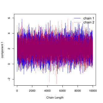
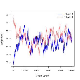
We compare the performance of RBM, ABM, and the naive estimator for two settings, $\rho=0.5,0.999$ with $\omega_{1}=\omega_{2}=1$. For Setting 1 ($\rho=.5$), the Markov chains travel freely across the state space so that in only a few steps, independent runs of the Markov chains from over-dispersed starting values look similar to each other. For Setting 2 $(\rho=.999)$, each Markov chain moves slowly across the state space. Trace plots in Figure 1 give evidence of this.

(a)

(b)

Figure 1: Bivariate normal: Trace plots of two parallel Markov chains.

We set $m=5,10$ for both the settings and first compare the evolution of the estimates of $\Sigma$ over time. Figure 2 presents the running plots of the Frobenius norm of the estimators with the black horizontal line being the truth. In all four plots, the high variability of the naive estimator is demonstrated, consistent with Theorem 5. For Setting 1, RBM and ABM are indistinguishable as was expected from the trace plots. However, the advantage of using RBM is evident in Setting 2, where the RBM estimator converges to the truth quicker than the ABM estimator. This is a direct consequence of the fact that slowly mixing Markov chains take a longer time to traverse the state space, implying that the means of all the chains are significantly different in small MCMC runs.

(a)

(b)

(c)

(d)

Figure 2: Bivariate normal: Frobenius norm running plots (with standard errors) over 100 replications.

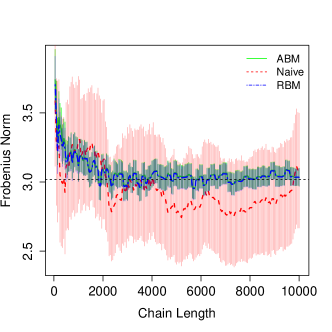
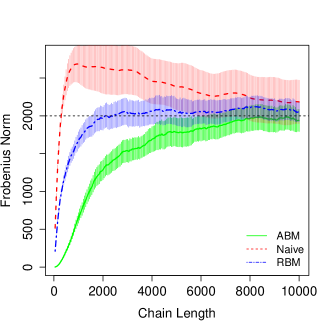
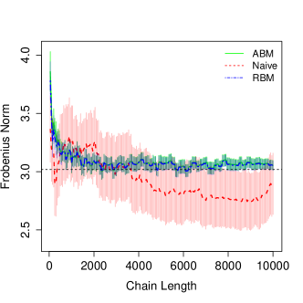
In order to quantify the effect of the quality of estimation of $\Sigma$, we estimate the coverage probabilities of the resulting $95\%$ confidence regions over 1000 replications for both settings. In addition to the coverage probabilities obtained using ABM, naive, and RBM, we also estimate the coverage probability using the true $\Sigma$; this, in some sense, represents the oracle. The results are presented in Table 1. For Setting 1 (for both $m=5,10$), ABM and RBM yield similar coverage, as was expected. Here, the high variability of the naive estimator impacts the coverage significantly which does not improve as $n$ increases, demonstrating the effect of Theorem 5. For Setting 2, there is a clear separation of coverage probabilities between RBM and ABM, especially for smaller sample sizes. As the sample size increases, ABM and RBM yield more similar coverage as a consequence of less separation between the means from each chain.

$n$	ABM	Naive	RBM	True
$1e2$	0.913	0.764	0.909	0.956
$5e2$	0.926	0.773	0.924	0.948
$1e3$	0.940	0.744	0.943	0.949
$1e4$	0.951	0.749	0.951	0.951

(a)

$n$	ABM	Naive	RBM	True
$1e2$	0.696	0.860	0.934	0.928
$5e2$	0.794	0.846	0.908	0.936
$1e3$	0.851	0.866	0.907	0.962
$1e4$	0.902	0.746	0.898	0.952

(b)

$n$	ABM	Naive	RBM	True
$1e2$	0.919	0.874	0.913	0.951
$5e2$	0.937	0.868	0.937	0.946
$1e3$	0.931	0.874	0.929	0.945
$1e4$	0.955	0.865	0.955	0.956

(c)

$n$	ABM	Naive	RBM	True
$1e2$	0.729	0.949	0.948	0.935
$5e2$	0.823	0.939	0.936	0.948
$1e3$	0.872	0.930	0.938	0.966
$1e4$	0.939	0.888	0.934	0.958

(d)

Table 1: Bivariate normal: Coverage probabilities from 1000 replications at 95% nominal level.

In the rest of the examples, we focus only on comparing the RBM to the ABM estimator, since it is evident that the naive estimator is unreliable.

4.2 Rosenbrock distribution

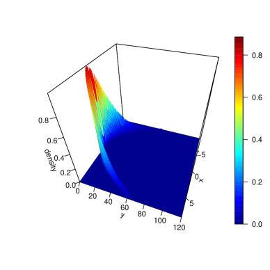
The Rosenbrock distribution is commonly used to serve as a benchmark for testing MCMC algorithms. As can be seen in Figure 3, the density takes positive values along a narrow parabola making it difficult for MCMC algorithms to take large steps. Consider the 2-dimensional Rosenbrock density discussed in Goodman and Weare, (2010) and Pagani et al., (2019):

$$\pi(x_{1},x_{2})\propto\exp\left\{-\dfrac{1}{20}(x_{1}-1)^{2}-5\left(x_{2}-x_{1}^{2}\right)^{2}\right\}\,.$$

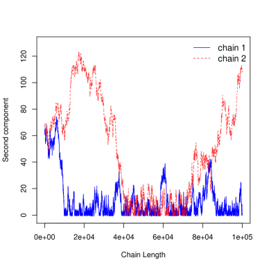
Although there are specialized MCMC algorithms available that traverse the contours of the Rosenbrock density more efficiently, we implement a random walk Metropolis-Hastings algorithm with a Gaussian proposal. Trace plots for one component of two runs are presented in Figure 3.

(a)

(b)

Figure 3: $2d$ Rosenbrock density and trace plots.

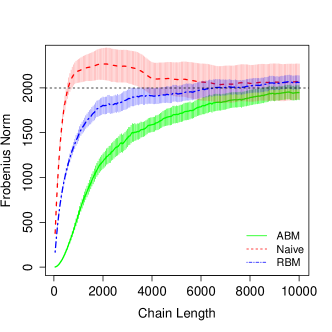
We set $m=5,10$ with evenly dispersed starting points. Since $\Sigma$ is unknown, we compare ABM and RBM by analyzing running plots of the estimated effective sample size (ESS). ESS is a popular tool for assessing when to terminate MCMC simulations by determining the number of iid samples that would yield the same standard error for the Monte Carlo estimator. Vats et al., (2019) define

$$\text{ESS}=mn\left(\dfrac{|\text{Var}_{F}(h(X_{11}))|}{|\Sigma|}\right)^{1/p}\,,$$

where $|\cdot|$ is the determinant. Simulation terminates when an estimated ESS, $\widehat{\text{ESS}}>M$, for a pre-specified $M$. To avoid early termination, it is critical that the estimate of $\Sigma$ is not underestimated.

(a)

(b)

Figure 4: Rosenbrock: $\widehat{\text{ESS}}/mn$ running plots (with standard errors).

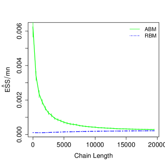
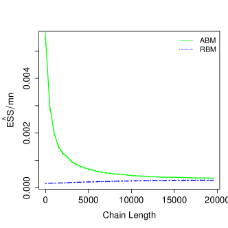
Figure 4 presents the estimated $\widehat{\text{ESS}}/mn$ over 100 replications using the average sample covariance matrix estimate of $\text{Var}_{F}(h(X_{11}))$ and ABM and RBM estimates of $\Sigma$. We observe that for both $m=5,10$, ABM grossly overestimates $\widehat{\text{ESS}}/mn$ and converges from above, whereas RBM converges from below. As a consequence, using RBM will help safeguard against early termination, whereas ABM is significantly more likely to produce inadequate estimates at termination.

Since the true mean for this target density is known, we compare coverage probabilities of the resulting confidence regions using ABM and RBM over 1000 replications in Table 2. The results for $m=5$ and $m=10$ are similar; the ABM estimator yields abysmally low coverage, especially at the beginning of the process. The RBM estimator, on the other hand, yields a high coverage probability despite the slow mixing nature of the Markov chain.

$n$	ABM	RBM
$5e3$	0.2	0.801
$10^{4}$	0.496	0.909
$5e4$	0.883	0.917
$10^{5}$	0.891	0.908

(a) $m=5$

$n$	ABM	RBM
$5e3$	0.181	0.743
$10^{4}$	0.479	0.876
$5e4$	0.846	0.891
$10^{5}$	0.864	0.879

(b) $m=10$

Table 2: Rosenbrock: Coverage probabilities over 1000 replications at 95% nominal level.

4.3 Bayesian multinomial regression

Consider the 1989 Dutch parliamentary election study (Anker and Oppenhuis,, 1993) which contains 1754 self-reported voting choices of survey respondents among four contesting parties and 11 explanatory variables. The dataset is available in Nethvote in the R package MCMCpack (Martin et al.,, 2011). We consider a Bayesian multinomial regression with four levels for the response variable, each for a contesting political party. Let $y_{i}$ and $x_{ij}$ denote the response variable and the $j$th covariate for the $i$th observation, respectively. Let $\beta$ denote the $22$-dimensional vector of regression coefficients and $\pi_{i}$ denote the 4-dimensional vector of probabilities for respondent $i$. Let

$$y_{i}\sim\text{Multinomial}(\pi_{i})\,,$$

where $\pi_{i}=(\pi_{i1},\pi_{i2},\pi_{i3},\pi_{i4})$ with

$$\pi_{ij}=\dfrac{\exp(x^{\prime}_{ij}\beta)}{\sum_{k=1}^{p}\exp(x^{\prime}_{ik}\beta)}\,.$$

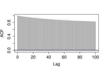
As considered by Martin et al., (2011), we set an improper prior for $\beta$, $f(\beta)\propto 1$. The resulting posterior distribution for $\beta$ is intractable and MCMC is needed to estimate the posterior mean. We use the MCMCmnl function in the R package MCMCpack which uses a random walk Metropolis-Hastings sampler with a Gaussian proposal distribution. We run 2 parallel Markov chains with starting values dispersed around the maximum likelihood estimator of $\beta$. The autocorrelation plots of randomly picked elements in Figure 5 shows significant autocorrelation in the Markov chain.

(a)

(b)

Figure 5: Multinomial: Autocorrelation plots for two randomly chosen components.

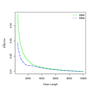
In this example, both the true posterior mean and the resulting asymptotic covariance matrix $\Sigma$ are unknown. Thus coverage probabilities are not estimable. We, therefore, focus on the quality of estimation of ESS. Figure 6 contains the running estimate of $\widehat{\text{ESS}}/mn$ using both ABM and RBM estimators. Since the target distribution is unimodal with moderate levels of posterior correlation, it does not take long for the two Markov chains to adequately explore the state space. Even then, there is a noticeable advantage of using RBM over ABM. RBM produces a systematically lower estimate of ESS whereas the ABM estimator may give a false sense of security in early small runs of the sampler. However, the two of them start agreeing after 5000 steps in the Markov chain, at which point RBM is no better than ABM. This agrees with our theoretical results which indicated that the large sample behavior of both methods is similar. Even in this simple Bayesian model, the finite sample gains of using the RBM estimator are undeniable.

Figure 6: Multinomial: $\widehat{\text{ESS}}/mn$ running plots averaged over 1000 replications.

5 Discussion

Work in MCMC output analysis has so far not caught up to the ease with which users can implement parallel MCMC runs. This work is a first attempt at consistent estimation of $\Sigma$ for parallel MCMC. For fast mixing Markov chains, the RBM estimator is as good as the current state-of-the-art, and for slow mixing chains, the RBM estimator provides significant improvement and safeguards users from premature termination of the process.

Choosing a batch size is a challenging problem for single-chain batch means, and the optimal batch size of Liu et al., (2018) is a step in the right direction. Since each realization of a Markov chain can yield different optimal batch sizes, an important future extension would be to construct RBM estimators from pooling batches of different batch sizes, each tuned to its own Markov chain. Additionally, here we consider only non-overlapping batch means estimators due to their computational feasibility. Similar construction for multiple-chain output analysis should be possible for the overlapping batch means estimators found in Flegal and Jones, (2010); Liu et al., (2018).

Appendix A Preliminaries

We present a few preliminary results to assist us in our proofs.

Lemma 1.

(Csorgo and Revesz (1981)). Suppose Assumption2 holds, then for all $\epsilon>0$ and for almost all sample paths, there exists $n_{0}\left(\epsilon\right)$ such that $\forall n\geq n_{0}$ and $\forall i=1,...,p$

$$\sup_{0\leq t\leq n-b}\sup_{0\leq s\leq b}\left|B^{\left(i\right)}\left(t+s\right)-B^{\left(i\right)}\left(t\right)\right|<\left(1+\epsilon\right)\left(2b\left(\log\dfrac{n}{b}+\log\;\log\;n\right)\right)^{1/2},$$

$$\sup_{0\leq s\leq b}\left|B^{\left(i\right)}\left(n\right)-B^{\left(i\right)}\left(n-s\right)\right|<\left(1+\epsilon\right)\left(2b\left(\log\dfrac{n}{b}+\log\;\log\;n\right)\right)^{1/2},\;and$$

$$\left|B^{\left(i\right)}\left(n\right)\right|<\left(1+\epsilon\right)\sqrt{2n\;\log\log n}\;.$$

The following straightforward decomposition will be used often and thus is presented as a lemma.

Lemma 2.

For $\hat{\mu}_{k}$ and $\hat{\mu}$ defined as before,

$$\sum\limits_{k=1}^{m}\left(\hat{\mu}_{k}-\hat{\mu}\right)\left(\hat{\mu}_{k}-\hat{\mu}\right)^{T}=\displaystyle\sum_{k=1}^{m}(\hat{\mu}_{k}-\mu)(\hat{\mu}_{k}-\mu)^{T}-m(\hat{\mu}-\mu)(\hat{\mu}-\mu)^{T}\,.$$

A.1 Strong consistency of RBM

Proof of Theorem 2.

We will show that the RBM estimator can be decomposed into the ABM estimator, plus some small order terms. Consider

$$\hat{\Sigma}_{R,b} =\dfrac{b}{am-1}\sum_{k=1}^{m}\sum_{s=1}^{a}\left(\bar{Y}_{k,s}-\hat{\mu}\right)\left(\bar{Y}_{k,s}-\hat{\mu}\right)^{T}$$

$$=\dfrac{b}{am-1}\sum_{k=1}^{m}\sum_{s=1}^{a}\left(\bar{Y}_{k,s}-\hat{\mu}_{k}+\hat{\mu}_{k}-\hat{\mu}\right)\left(\bar{Y}_{k,s}-\hat{\mu}_{k}+\hat{\mu}_{k}-\hat{\mu}\right)^{T}$$

$$=\dfrac{b}{am-1}\sum_{k=1}^{m}\sum_{s=1}^{a}\left[\left(\bar{Y}_{k,s}-\hat{\mu}_{k}\right)\left(\bar{Y}_{k,s}-\hat{\mu}_{k}\right)^{T}+\left(\bar{Y}_{k,s}-\hat{\mu}_{k}\right)\left(\hat{\mu}_{k}-\hat{\mu}\right)^{T}\right.$$

$$\quad\quad\left.+\left(\hat{\mu}_{k}-\hat{\mu}\right)\left(\bar{Y}_{k,s}-\hat{\mu}_{k}\right)^{T}+\left(\hat{\mu}_{k}-\hat{\mu}\right)\left(\hat{\mu}_{k}-\hat{\mu}\right)^{T}\right]$$

$$=\dfrac{b}{am-1}\dfrac{a-1}{b}\sum_{k=1}^{m}\hat{\Sigma}_{k,b}+\dfrac{b}{am-1}\sum_{k=1}^{m}\left[\sum_{s=1}^{a}\left(\bar{Y}_{k,s}-\hat{\mu}_{k}\right)\right]\left(\hat{\mu}_{k}-\hat{\mu}\right)^{T}$$

$$\quad\quad+\dfrac{b}{am-1}\sum_{k=1}^{m}\left(\hat{\mu}_{k}-\hat{\mu}\right)\sum_{s=1}^{a}\left(\bar{Y}_{k,s}-\hat{\mu}_{k}\right)^{T}+\dfrac{ab}{am-1}\sum_{k=1}^{m}\left(\hat{\mu}_{k}-\hat{\mu}\right)\left(\hat{\mu}_{k}-\hat{\mu}\right)^{T}$$

$$=\dfrac{m(a-1)}{am-1}\hat{\Sigma}_{A,b}+\dfrac{ab}{am-1}\sum_{k=1}^{m}\left(\hat{\mu}_{k}-\hat{\mu}\right)\left(\hat{\mu}_{k}-\hat{\mu}\right)^{T}\,.$$ (6)

By Lemma 2

$$\dfrac{ab}{am-1}\sum_{k=1}^{m}\left(\hat{\mu}_{k}-\hat{\mu}\right)\left(\hat{\mu}_{k}-\hat{\mu}\right)^{T} =\dfrac{ab}{am-1}\sum_{k=1}^{m}\left(\hat{\mu}_{k}-\mu\right)\left(\hat{\mu}_{k}-\mu\right)^{T}-\dfrac{abm}{am-1}\left(\hat{\mu}-\mu\right)\left(\hat{\mu}-\mu\right)^{T}$$

Let

$$A=\dfrac{a}{am-1}\sum_{k=1}^{m}b\left(\hat{\mu}_{k}-\mu\right)\left(\hat{\mu}_{k}-\mu\right)^{T}\quad\text{ and }\quad B=\dfrac{abm}{am-1}\left(\hat{\mu}-\mu\right)\left(\hat{\mu}-\mu\right)^{T}\,.$$

By Strassen, (1964), $\psi(n)=O(\sqrt{n\log\log n})$ so that the rate is such that the law of iterated logarithm holds. Let $A^{ij}$, be the $(i,j)$th element of the matrix $A$. Using the SIP and Lemma 1,

$$\left|A^{ij}\right| =\dfrac{a}{am-1}\sum_{k=1}^{m}\left|b\left(\bar{Y}^{\left(i\right)}_{k}-\mu^{(i)}\right)\left(\bar{Y}^{\left(j\right)}_{k}-\mu^{(j)}\right)\right|$$

$$\leq\dfrac{a}{am-1}\sum_{k=1}^{m}\left[\left|\dfrac{b}{n^{2}}\left(\sum_{r=1}^{n}Y^{\left(i\right)}_{r,k}-n\mu^{(i)}\right)\left(\sum_{s=1}^{n}Y^{\left(j\right)}_{s,k}-n\mu^{(j)}\right)\right|\right]$$

$$=\dfrac{a}{am-1}\sum_{k=1}^{m}\left[\dfrac{b}{n^{2}}\left|\left(\sum_{r=1}^{n}Y^{\left(i\right)}_{r,k}-n\mu^{(i)}-\Sigma_{ii}B^{\left(i\right)}+\Sigma_{ii}B^{\left(i\right)}\right)\left(\sum_{s=1}^{n}Y^{\left(j\right)}_{s,k}-n\mu^{(j)}-\Sigma_{jj}B^{\left(j\right)}+\Sigma_{jj}B^{\left(j\right)}\right)\right|\right]$$

$$\leq\dfrac{a}{am-1}\sum_{k=1}^{m}\left[\dfrac{b}{n^{2}}\left[\left|\left(\sum_{r=1}^{n}Y^{\left(i\right)}_{r,k}-n\mu^{(i)}-\Sigma_{ii}B^{\left(i\right)}\right)\left(\sum_{s=1}^{n}Y^{\left(j\right)}_{s,k}-n\mu^{(j)}-\Sigma_{jj}B^{\left(j\right)}\right)\right|\right.\right.$$

$$\left.\left.\quad+\left|\left(\Sigma_{ii}B^{\left(i\right)}\right)\right|\left|\left(\sum_{s=1}^{n}Y^{\left(j\right)}_{s,k}-n\mu^{\left(j\right)}-\Sigma_{jj}B^{\left(j\right)}\right)\right|+\left|\left(\Sigma_{jj}B^{\left(j\right)}\right)\right|\left|\left(\sum_{r=1}^{n}Y^{\left(i\right)}_{r,k}-n\mu^{(i)}-\Sigma_{ii}B^{\left(i\right)}\right)\right|\right.\right.$$

$$\quad+\left|\left(\Sigma_{ii}B^{\left(i\right)}\right)\right|\left|\left(\Sigma_{jj}B^{\left(j\right)}\right)\right|\Bigg{]}\Bigg{]}$$

$$<\dfrac{a}{am-1}\sum_{k=1}^{m}\left[\dfrac{b}{n^{2}}\left[\left(D\psi\left(n\right)\right)^{2}+\Sigma_{ii}\left(1+\epsilon\right)\sqrt{2n\log\log n}\left(D\psi\left(n\right)\right)\right.\right.$$

$$\quad\left.+\Sigma_{jj}\left(1+\epsilon\right)\sqrt{2n\log\log n}\left(D\psi\left(n\right)\right)+\Sigma_{ii}\Sigma_{jj}\left(1+\epsilon\right)^{2}\left(2n\log\log n\right)\right]\Bigg{]}$$

$$=\dfrac{am}{am-1}\left[\dfrac{b}{n}\left(\dfrac{D\psi\left(n\right)}{\sqrt{n}}\right)^{2}+\left(\Sigma_{ii}+\Sigma_{jj}\right)\left(1+\epsilon\right)\dfrac{b\sqrt{2\log\log n}}{n}\left(\dfrac{D\psi\left(n\right)}{\sqrt{n}}\right)\right.$$

$$\quad+\left.2\Sigma_{ii}\Sigma_{jj}\left(1+\epsilon\right)^{2}\left(\dfrac{b\log\log n}{n}\right)\right]$$

$$=\dfrac{am}{am-1}\dfrac{b\log\log n}{n}\left[\left(\dfrac{D\psi\left(n\right)}{\sqrt{n\log\log n}}\right)^{2}+\sqrt{2}\left(\Sigma_{ii}+\Sigma_{jj}\right)\left(1+\epsilon\right)\left(\dfrac{D\psi\left(n\right)}{\sqrt{n\log\log n}}\right)+2\Sigma_{ii}\Sigma_{jj}\left(1+\epsilon\right)^{2}\right]$$

$$\xrightarrow{a.s}0\;\;n\to\infty\,.$$

Following the same steps for $B^{ij}$ with $n$ replaced by $mn$, $\left|B^{ij}\right|\xrightarrow{a.s}0\;\;n\to\infty$. Therefore $\|A\|\xrightarrow{a.s}\mathbf{0}$ and $\|B\|\xrightarrow{a.s}\mathbf{0}$ as $n\to\infty$. Using this,

$$\left|\left|\dfrac{ab}{am-1}\sum_{k=1}^{m}\left(\hat{\mu}_{k}-\hat{\mu}\right)\left(\hat{\mu}_{k}-\hat{\mu}\right)^{T}\right|\right|=\left|\left|A-B\right|\right|\leq\|A\|+\|B\|\xrightarrow{a.s}\mathbf{0}\;\;n\to\infty\,.$$ (7)

Using (7) and consistency of $\hat{\Sigma}_{k,b}$ for all $k$ in (6)

$$\left|\left|\hat{\Sigma}_{R,b}-\Sigma\right|\right| =\left|\left|\dfrac{m(a-1)}{am-1}\hat{\Sigma}_{A,b}-\Sigma+\dfrac{ab}{am-1}\sum_{k=1}^{m}\left(\hat{\mu}_{k}-\hat{\mu}\right)\left(\hat{\mu}_{k}-\hat{\mu}\right)^{T}\right|\right|$$

$$\leq\left|\left|\dfrac{m(a-1)}{am-1}\hat{\Sigma}_{A,b}-\Sigma\right|\right|+\left|\left|\dfrac{ab}{am-1}\sum_{k=1}^{m}\left(\hat{\mu}_{k}-\hat{\mu}\right)\left(\hat{\mu}_{k}-\hat{\mu}\right)^{T}\right|\right|$$

$$\overset{a.s.}{\to}0\quad\text{ as }n\to\infty\,.$$

∎

A.2 Bias of RBM

Proof of Theorem 3.

First, using Lemmas 1-3 of (Song and Schmeiser,, 1995),

$$\mathbb{E}\left[\sum\limits_{k=1}^{m}\left(\hat{\mu}_{k}-\hat{\mu}\right)\left(\hat{\mu}_{k}-\hat{\mu}\right)^{T}\right] =\mathbb{E}\left[\sum_{k=1}^{m}\hat{\mu}_{k}\hat{\mu}_{k}^{T}-\sum_{k=1}^{m}\hat{\mu}_{k}\hat{\mu}^{T}-\hat{\mu}\sum_{k=1}^{m}\hat{\mu}_{k}^{T}+m\hat{\mu}\hat{\mu}^{T}\right]$$

$$=\mathbb{E}\left[\sum_{k=1}^{m}\hat{\mu}_{k}\hat{\mu}_{k}^{T}-m\hat{\mu}\hat{\mu}^{T}\right]$$

$$=m\left(\mathbb{E}\left[\bar{Y}_{1}\bar{Y}_{1}^{T}\right]-\mathbb{E}\left[\hat{\mu}\hat{\mu}^{T}\right]\right)$$

$$=m\left(\text{Var}\left(\bar{Y}_{1}\right)-\text{Var}\left(\hat{\mu}\right)\right)$$

$$=m\left[\dfrac{\Sigma}{n}+\dfrac{\Gamma}{n^{2}}+o\left(\dfrac{1}{n^{2}}\right)-\dfrac{\Sigma}{mn}-\dfrac{\Gamma}{mn^{2}}+o\left(\dfrac{1}{mn^{2}}\right)\right]$$

$$=m\left[\dfrac{\Sigma}{n}\left(1-\dfrac{1}{m}\right)+\dfrac{\Gamma}{n^{2}}\left(1-\dfrac{1}{m}\right)+o\left(\dfrac{1}{n^{2}}\right)\right]\,.$$ (8)

By (6), (8), and the bias of the BM estimator from Vats and Flegal, (2018, Theorem 1),

$$\mathbb{E}[\hat{\Sigma}_{R,b}] =\mathbb{E}\left[\dfrac{a-1}{am-1}\sum_{k=1}^{m}\hat{\Sigma}_{k,b}+\dfrac{ab}{am-1}\sum_{k=1}^{m}\left(\hat{\mu}_{k}-\hat{\mu}\right)\left(\hat{\mu}_{k}-\hat{\mu}\right)^{T}\right]$$

$$=\dfrac{m\left(a-1\right)}{am-1}\mathbb{E}\left[\hat{\Sigma}_{k,1}\right]+\dfrac{abm}{am-1}\left(\dfrac{\Sigma}{n}\left(1-\dfrac{1}{m}\right)+\dfrac{\Gamma}{n^{2}}\left(1-\dfrac{1}{m}\right)+o\left(\dfrac{1}{n^{2}}\right)\right)$$

$$=\dfrac{m\left(a-1\right)}{am-1}\left[\Sigma+\dfrac{\Gamma}{b}+o\left(\dfrac{1}{b}\right)\right]+\dfrac{m\Sigma}{am-1}\left(1-\dfrac{1}{m}\right)+\dfrac{m\Gamma}{n\left(am-1\right)}\left(1-\dfrac{1}{m}\right)+\dfrac{m}{am-1}o\left(\dfrac{1}{n}\right)$$

$$=\dfrac{m\Sigma}{am-1}\left[\left(a-1\right)+1-\dfrac{1}{m}\right]+\dfrac{m\Gamma}{am-1}\left(\dfrac{a-1}{b}+\dfrac{1}{n}\left(1-\dfrac{1}{m}\right)\right)+o\left(\dfrac{1}{b}\right)$$

$$=\Sigma+\dfrac{m\left(a-1\right)\Gamma}{\left(am-1\right)b}+\dfrac{m\Gamma}{n\left(am-1\right)}\left(1-\dfrac{1}{m}\right)+o\left(\dfrac{1}{b}\right)$$

$$=\Sigma+\dfrac{\Gamma\left(am-1+1-m\right)}{\left(am-1\right)b}+o\left(\dfrac{1}{b}\right)$$

$$=\Sigma+\dfrac{\Gamma}{b}+o\left(\dfrac{1}{b}\right)\;.$$

∎

A.3 Variance of RBM

Recall that $\hat{\Sigma}_{R,L}$ is the lugsail RBM estimator and $\hat{\Sigma}_{A,l}$ is the lugsail averaged batch means estimator. Further, let $\hat{\Sigma}^{ij}_{R,L}$ and $\hat{\Sigma}^{ij}_{A,L}$ be the $\left(i,j\right)$th element of the matrices, respectively. We will prove that the variance of both the estimators is equivalent for large sample sizes. Due to the strong consistency proof, as $n\to\infty$,

$$\left|\left|\hat{\Sigma}_{R,L}-\dfrac{m\left(a-1\right)}{am-1}\hat{\Sigma}_{A,l}\right|\right|\to 0\text{ with probability 1}\,.$$ (9)

For ease of notation, set $C=m\left(a-1\right)/\left(am-1\right)$. Further, define

$$g_{1}\left(n\right) =2\left(\dfrac{1}{1-c}\dfrac{am}{am-1}+\dfrac{c}{1-c}\dfrac{am}{arm-1}\right)\dfrac{b\psi\left(n\right)^{2}}{n^{2}}$$

$$g_{2}\left(n\right) =2\left(\dfrac{1}{1-c}\dfrac{am}{am-1}+\dfrac{c}{1-c}\dfrac{am}{arm-1}\right)\left(\Sigma_{ii}+\Sigma_{jj}\right)\left(1+\epsilon\right)\dfrac{b\psi\left(n\right)\sqrt{2n\log\log n}}{n^{2}}$$

$$g_{3}\left(n\right) =2\left(\dfrac{1}{1-c}\dfrac{am}{am-1}+\dfrac{c}{1-c}\dfrac{am}{arm-1}\right)\Sigma_{ii}\Sigma_{jj}\left(1+\epsilon\right)^{2}\dfrac{2b\log\log n}{n}\,.$$

Since $\psi(n)=O(\sqrt{n\log\log n})$, if $\left(b\log\log n\right)/n\to 0$, then $g_{1},g_{2},g_{3}\to 0$. From the steps in Theorem 2,

$$\left|\hat{\Sigma}_{R,L}^{ij}-C\hat{\Sigma}_{A,L}^{ij}\right|$$

$$=\left|\dfrac{1}{1-c}\left(\hat{\Sigma}_{R,b}^{ij}-C\hat{\Sigma}_{A,b}^{ij}\right)-\dfrac{c}{1-c}\left(\hat{\Sigma}_{R,b/r}^{ij}-C\hat{\Sigma}_{A,b/r}^{ij}\right)\right|$$

$$=\left|\dfrac{1}{1-c}\left(\dfrac{ab}{am-1}\sum_{k=1}^{m}\left(\hat{\mu}_{k}^{(i)}-\hat{\mu}^{(i)}\right)\left(\hat{\mu}_{k}^{(j)}-\hat{\mu}^{(j)}\right)^{T}\right)-\dfrac{c}{1-c}\left(\dfrac{ab}{arm-1}\sum_{k=1}^{m}\left(\hat{\mu}_{k}^{(i)}-\hat{\mu}^{(i)}\right)\left(\hat{\mu}_{k}^{(j)}-\hat{\mu}^{(j)}\right)^{T}\right)\right|$$

$$\leq\dfrac{1}{1-c}\dfrac{ab}{am-1}\left|\sum_{k=1}^{m}\left(\hat{\mu}_{k}^{(i)}-\hat{\mu}^{(i)}\right)\left(\hat{\mu}_{k}^{(j)}-\hat{\mu}^{(j)}\right)^{T}\right|+\dfrac{c}{1-c}\dfrac{ab}{arm-1}\left|\sum_{k=1}^{m}\left(\hat{\mu}_{k}^{(i)}-\hat{\mu}^{(i)}\right)\left(\hat{\mu}_{k}^{(j)}-\hat{\mu}^{(j)}\right)^{T}\right|$$

$$=\left(\dfrac{1}{1-c}\dfrac{ab}{am-1}+\dfrac{c}{1-c}\dfrac{ab}{arm-1}\right)\left|\sum_{k=1}^{m}\left(\hat{\mu}_{k}^{(i)}-\hat{\mu}^{(i)}\right)\left(\hat{\mu}_{k}^{(j)}-\hat{\mu}^{(j)}\right)^{T}\right|$$

$$\leq D^{2}g_{1}\left(n\right)+Dg_{2}\left(n\right)+g_{3}\left(n\right)\,.$$

By (9), there exists an $N_{0}$ such that

$$\left(\hat{\Sigma}_{R,L}^{ij}-C\hat{\Sigma}_{A,L}^{ij}\right)^{2} =\left(\hat{\Sigma}_{R,L}^{ij}-C\hat{\Sigma}_{A,L}^{ij}\right)^{2}\,I\left(0\leq n\leq N_{0}\right)+\left(\hat{\Sigma}_{R,L}^{ij}-C\hat{\Sigma}_{A,L}^{ij}\right)^{2}\,I\left(n>N_{0}\right)$$

$$\leq\left(\hat{\Sigma}_{R,L}^{ij}-C\hat{\Sigma}_{A,L}^{ij}\right)^{2}\,I\left(0\leq n\leq N_{0}\right)+\left(D^{2}g_{1}\left(n\right)+Dg_{2}\left(n\right)+g_{3}\left(n\right)\right)^{2}I\left(n>N_{0}\right)$$

$$:=g_{n}^{*}\left(X_{11},\dots,X_{1n},\dots,X_{m1},\dots,X_{mn}\right)\,.$$

But since by assumption $\text{E}D^{4}<\infty$, $\text{E}\|h\|^{4}<\infty$,

$$\text{E}\left|g_{n}^{*}\right|\leq\text{E}\left[\left(\hat{\Sigma}_{R,L}^{ij}-C\hat{\Sigma}_{A,L}^{ij}\right)^{2}\right]+\text{E}\left[\left(D^{2}g_{1}\left(n\right)+Dg_{2}\left(n\right)+g_{3}\left(n\right)\right)^{2}\right]<\infty\,.$$

Thus, $\text{E}\left|g_{n}^{*}\right|<\infty$ and further as $n\to\infty$, $g_{n}\to 0$ under the assumptions. Since $g_{1},g_{2},g_{3}\to 0$, $\text{E}g_{n}^{*}\to 0$. By the majorized convergence theorem (Zeidler,, 2013), as $n\to\infty$,

$$\text{E}\left[\left(\hat{\Sigma}_{R,L}^{ij}-C\hat{\Sigma}_{A,L}^{ij}\right)^{2}\right]\to 0\,.$$ (10)

We will use (10) to show that the variances are equivalent. Define,

$$\Omega\left(\hat{\Sigma}_{R,L}^{ij},\hat{\Sigma}_{A,L}^{ij}\right)=\text{Var}\left(\hat{\Sigma}_{R,L}^{ij}-C\hat{\Sigma}_{A,L}^{ij}\right)+2C\text{E}\left[\left(\hat{\Sigma}_{R,L}^{ij}-C\hat{\Sigma}_{A,L}^{ij}\right)\left(\hat{\Sigma}_{A,L}^{ij}-\text{E}\left(\hat{\Sigma}_{A,L}^{ij}\right)\right)\right]\;.$$

We will show that the above is $o\left(1\right)$. Using Cauchy-Schwarz inequality followed by (10),

$$\left|\Omega\left(\hat{\Sigma}_{R,L}^{ij},\hat{\Sigma}_{A,L}^{ij}\right)\right|$$

$$\leq\left|\text{Var}\left(\hat{\Sigma}_{R,L}^{ij}-C\hat{\Sigma}_{A,L}^{ij}\right)\right|+\left|2C\text{E}\left[\left(\hat{\Sigma}_{R,L}^{ij}-C\hat{\Sigma}_{A,L}^{ij}\right)\left(\hat{\Sigma}_{A,L}^{ij}-\text{E}\left(\hat{\Sigma}_{A,L}^{ij}\right)\right)\right]\right|$$

$$=\text{E}\left[\left(\hat{\Sigma}_{R,L}^{ij}-C\hat{\Sigma}_{A,L}^{ij}\right)^{2}\right]+2C\left|\left(\text{E}\left[\left(\hat{\Sigma}_{R,L}^{ij}-C\hat{\Sigma}_{A,L}^{ij}\right)^{2}\right]\text{Var}\left(\hat{\Sigma}_{A,L}^{ij}\right)\right)^{1/2}\right|$$

$$=o\left(1\right)+2C\left(o\left(1\right)\left(O\left(\dfrac{b}{n}\right)+o\left(\dfrac{b}{n}\right)\right)\right)$$

$$=o\left(1\right)\,.$$

Finally,

$$\text{Var}\left(\hat{\Sigma}_{R,L}^{ij}\right)$$

$$=\text{E}\left[\left(\hat{\Sigma}_{R,L}^{ij}-\text{E}\left[\hat{\Sigma}_{R,L}^{ij}\right]\right)^{2}\right]$$

$$=\text{E}\left[\left(\hat{\Sigma}_{R,L}^{ij}\pm C\hat{\Sigma}_{A,L}^{ij}\pm C\text{E}\left[\hat{\Sigma}_{A,L}^{ij}\right]-\text{E}\left[\hat{\Sigma}_{R,L}^{ij}\right]\right)^{2}\right]$$

$$=\text{E}\left[\left(\left(\hat{\Sigma}_{R,L}^{ij}-C\hat{\Sigma}_{A,L}^{ij}\right)+C\left(\hat{\Sigma}_{A,L}^{ij}-\text{E}\left[\hat{\Sigma}_{A,L}^{ij}\right]\right)+\left(C\text{E}\left[\hat{\Sigma}_{A,L}^{ij}\right]-\text{E}\left[\hat{\Sigma}_{R,L}^{ij}\right]\right)\right)^{2}\right]$$

$$=C^{2}\text{E}\left[\left(\hat{\Sigma}_{A,L}^{ij}-\text{E}\left[\hat{\Sigma}_{A,L}^{ij}\right]\right)^{2}\right]+\text{E}\left[\left(\left(\hat{\Sigma}_{R,L}^{ij}-C\hat{\Sigma}_{A,L}^{ij}\right)+\left(C\text{E}\left[\hat{\Sigma}_{A,L}^{ij}\right]-\text{E}\left[\hat{\Sigma}_{R,L}^{ij}\right]\right)\right)^{2}\right]$$

$$\quad\quad+2C\text{E}\left[\left(\hat{\Sigma}_{A,L}^{ij}-\text{E}\left[\hat{\Sigma}_{A,L}^{ij}\right]\right)\left(\hat{\Sigma}_{R,L}^{ij}-C\hat{\Sigma}_{A,L}^{ij}\right)\right]+2C\text{E}\left[\left(\hat{\Sigma}_{A,L}^{ij}-\text{E}\left[\hat{\Sigma}_{A,L}^{ij}\right]\right)\left(C\text{E}\left[\hat{\Sigma}_{A,L}^{ij}\right]-\text{E}\left[\hat{\Sigma}_{R,L}^{ij}\right]\right)\right]$$

$$=C^{2}\text{Var}\left(\hat{\Sigma}_{A,L}^{ij}\right)+\text{Var}\left(\hat{\Sigma}_{R,L}^{ij}-C\hat{\Sigma}_{A,L}^{ij}\right)+2C\text{E}\left[\left(\hat{\Sigma}_{R,L}^{ij}-C\hat{\Sigma}_{A,L}^{ij}\right)\left(\hat{\Sigma}_{A,L}^{ij}-\text{E}\left(\hat{\Sigma}_{A,L}^{ij}\right)\right)\right]+o\left(1\right)$$

$$=C^{2}\text{Var}\left(\hat{\Sigma}_{A,L}^{ij}\right)+\Omega\left(\hat{\Sigma}_{R,L}^{ij},\hat{\Sigma}_{A,L}^{ij}\right)+o\left(1\right)$$

$$=C^{2}\text{Var}\left(\hat{\Sigma}_{A,L}^{ij}\right)+o\left(1\right)+o\left(1\right)\,.$$

Thus,

$$\text{Var}\left(\hat{\Sigma}_{R,L}^{ij}\right) =\dfrac{m^{2}\left(a-1\right)^{2}}{\left(am-1\right)^{2}}\text{Var}\left(\hat{\Sigma}_{A,L}^{ij}\right)+o\left(1\right)$$

$$=\dfrac{m\left(a-1\right)^{2}}{\left(am-1\right)^{2}}\text{Var}\left(\hat{\Sigma}_{B,l}^{ij}\right)+o\left(1\right)$$

$$=\dfrac{m\left(a-1\right)^{2}}{\left(am-1\right)^{2}}\left[\dfrac{b}{n}\left(\dfrac{1}{r}+\dfrac{r-1}{r\left(1-c\right)^{2}}\right)\left(\Sigma^{2}_{ij}+\Sigma_{ii}\Sigma_{jj}\right)+o\left(\dfrac{b}{n}\right)\right]+o\left(1\right)$$

$$=\dfrac{m\left(a-1\right)^{2}}{a\left(am-1\right)^{2}}\left[\left(\dfrac{1}{r}+\dfrac{r-1}{r\left(1-c\right)^{2}}\right)\left(\Sigma^{2}_{ij}+\Sigma_{ii}\Sigma_{jj}\right)\right]+o\left(1\right)$$

$$=\dfrac{m^{2}\left(a-1\right)^{2}}{am\left(am-1\right)^{2}}\left[\left(\dfrac{1}{r}+\dfrac{r-1}{r\left(1-c\right)^{2}}\right)\left(\Sigma^{2}_{ij}+\Sigma_{ii}\Sigma_{jj}\right)\right]+o\left(1\right)$$

$$=\left(\dfrac{\left(am\right)^{2}+m^{2}-2am^{2}}{am\left(am-1\right)^{2}}\right)\left[\left(\dfrac{1}{r}+\dfrac{r-1}{r\left(1-c\right)^{2}}\right)\left(\Sigma^{2}_{ij}+\Sigma_{ii}\Sigma_{jj}\right)\right]+o\left(1\right)$$

$$=\left(\dfrac{\left(\left(am\right)^{2}-2am+1+2am-1+m^{2}-2am^{2}\right)}{am\left(am-1\right)^{2}}\right)\left[\left(\dfrac{1}{r}+\dfrac{r-1}{r\left(1-c\right)^{2}}\right)\left(\Sigma^{2}_{ij}+\Sigma_{ii}\Sigma_{jj}\right)\right]+o\left(1\right)$$

$$=\left(\dfrac{1}{am}-\dfrac{2\left(m-1\right)}{\left(am-1\right)^{2}}+\dfrac{m^{2}-1}{am\left(am-1\right)^{2}}\right)\left[\left(\dfrac{1}{r}+\dfrac{r-1}{r\left(1-c\right)^{2}}\right)\left(\Sigma^{2}_{ij}+\Sigma_{ii}\Sigma_{jj}\right)\right]+o\left(1\right)$$

$$=\dfrac{1}{am}\left[\left(\dfrac{1}{r}+\dfrac{r-1}{r\left(1-c\right)^{2}}\right)\left(\Sigma^{2}_{ij}+\Sigma_{ii}\Sigma_{jj}\right)\right]+o\left(1\right)$$

$$=\dfrac{b}{mn}\left[\left(\dfrac{1}{r}+\dfrac{r-1}{r\left(1-c\right)^{2}}\right)\left(\Sigma^{2}_{ij}+\Sigma_{ii}\Sigma_{jj}\right)\right]+o\left(1\right)\;.$$

A.4 Proof of Theorem 5

Proof of Theorem 5.

The proof follows from the fact that under Assumption 1, a CLT holds for both $\hat{\mu}_{k}$ and $\hat{\mu}$. That is,

$$\sqrt{n}(\hat{\mu}_{k}-\mu)\overset{d}{\to}N(0,\Sigma)\,\quad\text{ and }\quad\sqrt{mn}(\hat{\mu}-\mu)\overset{d}{\to}N(0,\Sigma)\,.$$

By Lemma 2,

$$\hat{\Sigma}_{N} =\dfrac{1}{m-1}\left[n\displaystyle\sum_{k=1}^{m}(\hat{\mu}_{k}-\mu)(\hat{\mu}_{k}-\mu)^{T}-mn(\hat{\mu}-\mu)(\hat{\mu}-\mu)^{T}\right]$$

$$=\dfrac{1}{m-1}\left[\displaystyle\sum_{k=1}^{m}\sqrt{n}(\hat{\mu}_{k}-\mu)\sqrt{n}(\hat{\mu}_{k}-\mu)^{T}-\sqrt{mn}(\hat{\mu}-\mu)\sqrt{mn}(\hat{\mu}-\mu)^{T}\right]\,.$$

By a standard argument of asymptotic independence of $\hat{\Sigma}_{N}$ and $\hat{\mu}$,

$$\hat{\Sigma}_{N}\overset{d}{\to}W_{p}(\Sigma,m-1)/(m-1)\,.$$

∎

A.5 Bivariate Normal Gibbs Asymptotic Variance

The diagonals of $\Sigma$ are indirectly obtained by Geyer, (1995) using a slightly different proof technique. For $t\geq 0$, let $\epsilon_{1,t}\sim N\left(0,\omega_{1}-\rho^{2}/{\omega_{2}}\right)$ and let $\epsilon_{2,t}\sim N(0,\omega_{2}-\rho^{2}/\omega_{1})$, independent of each other. For a given state at time $t-1$, the next state is drawn from

$$X_{1,t}=\mu_{1}+\dfrac{\rho}{\omega_{2}}\left(X_{2,t-1}-\mu_{2}\right)+\epsilon_{1,t}\,$$ (11)

$$X_{2,t}=\mu_{2}+\dfrac{\rho}{\omega_{1}}\left(X_{1,t}-\mu_{1}\right)+\epsilon_{2,t}$$ (12)

Additionally, for $t\geq 1$, define,

$$w_{t}=\dfrac{\rho}{\omega_{2}}\epsilon_{2,t-1}+\epsilon_{1,t}\sim N\left(0,\omega_{1}\left(1-\dfrac{\rho^{4}}{\omega_{1}^{2}\omega_{2}^{2}}\right)\right)\,.$$

Substituting $X_{2,t-1}$ from (12) to (11) gives,

$$X_{1,t} =\mu_{1}+\dfrac{\rho}{\omega_{2}}\left(\dfrac{\rho}{\omega_{1}}X_{1,t-1}-\dfrac{\rho}{\omega_{1}}\mu_{1}+\epsilon_{2,t-1}\right)+\epsilon_{1,t}$$

$$=\mu_{1}+\dfrac{\rho^{2}}{\omega_{1}\omega_{2}}X_{1,t-1}-\dfrac{\rho^{2}}{\omega_{1}\omega_{2}}\mu_{1}+\dfrac{\rho}{\omega_{2}}\epsilon_{2,t-1}+\epsilon_{1,t}$$

$$=\mu_{1}\left(1-\dfrac{\rho^{2}}{\omega_{1}\omega_{2}}\right)+\dfrac{\rho^{2}}{\omega_{1}\omega_{2}}X_{1,t-1}+w_{t}\,.$$ (13)

This is an autoregressive process of order 1 (AR(1) process). The process is also stationary by the assumption that $\rho^{2}<\omega_{1}\omega_{2}$ and the stationary distribution is $N(\mu_{1},\omega_{1})$. Thus $\text{Var}(X_{1})=\omega_{1}$ and similarly $\text{Var}(X_{2})=\omega_{2}$. Using the properties of an AR(1) process,

$$\text{Cov}\left(X_{1,1},X_{1,1+k}\right)=\text{Var}\left(X_{1}\right)\left(\dfrac{\rho^{2}}{\omega_{1}\omega_{2}}\right)^{k}=\omega_{1}\left(\dfrac{\rho^{2}}{\omega_{1}\omega_{2}}\right)^{k}\,.$$

The diagonal terms of the asymptotic covariance matrix for $i=1,2$ are

$$\Sigma_{ii}=\lim_{n\to\infty}n\text{Var}\left(\dfrac{1}{n}\sum_{t=1}^{n}X_{i,t}\right)\,.$$

Without loss of generality, consider $i=1$

$$\Sigma_{11} =\text{Var}\left(X_{1}\right)+2\sum_{k=1}^{\infty}\text{Cov}\left(X_{1,1},X_{1,1+k}\right)$$

$$=\omega_{1}+2\sum_{j=2}^{\infty}\omega_{1}\left(\dfrac{\rho^{2}}{\omega_{1}\omega_{2}}\right)^{k}=\omega_{1}\left(\dfrac{\omega_{1}\omega_{2}+\rho^{2}}{\omega_{1}\omega_{2}-\rho^{2}}\right)\;.$$

Similarly,

$$\Sigma_{22}=\omega_{2}\left(\dfrac{\omega_{1}\omega_{2}+\rho^{2}}{\omega_{1}\omega_{2}-\rho^{2}}\right)\;.$$

Consider the off-diagonal terms,

$$\Sigma_{12}=\Sigma_{21}=\text{Cov}(X_{1,1},X_{2,1})+\sum_{k=1}^{\infty}\left[\text{Cov}\left(X_{1,1},X_{2,1+k}\right)+\text{Cov}\left(X_{2,1},X_{1,1+k}\right)\right]\,.$$ (14)

We have $\text{Cov}\left(X_{1,1},X_{2,1+k}\right)=\mathbb{E}(X_{1,1}X_{2,1+k})-\mu_{1}\mu_{2}$ and using (5),

$$\mathbb{E}\left(X_{1,1}X_{2,1+k}\right) =\mathbb{E}\left[X_{1,1}\left(\mu_{2}-\dfrac{\rho}{\omega_{1}}\mu_{1}+\dfrac{\rho}{\omega_{1}}X_{1,1+k}+\epsilon_{2,1+k}\right)\right]$$

$$=\mu_{1}\mu_{2}-\dfrac{\rho}{\omega_{1}}\mu_{1}^{2}+\dfrac{\rho}{\omega_{1}}\mathbb{E}\left(X_{1,1}X_{1,1+k}\right)+0$$

$$=\mu_{1}\mu_{2}-\dfrac{\rho}{\omega_{1}}\mu_{1}^{2}+\dfrac{\rho}{\omega_{1}}\left[\text{Cov}\left(X_{1,1},X_{1,1+k}\right)+\mathbb{E}\left(X_{1,1}\right)\mathbb{E}\left(X_{1,1+k}\right)\right]$$

$$=\mu_{1}\mu_{2}-\dfrac{\rho}{\omega_{1}}\mu_{1}^{2}+\dfrac{\rho}{\omega_{1}}\left(\omega_{1}\left(\dfrac{\rho^{2}}{\omega_{1}\omega_{2}}\right)^{k}+\mu_{1}^{2}\right)$$

$$=\mu_{1}\mu_{2}+\rho\left(\dfrac{\rho^{2}}{\omega_{1}\omega_{2}}\right)^{k}\,.$$ (15)

Similarly, simplification of $\mathbb{E}\left(X_{1,1}X_{2,1+k}\right)$ using (4) gives

$$\mathbb{E}\left(X_{2,1}X_{1,1+k}\right) =\mathbb{E}\left[X_{2,1}\left(\mu_{1}-\dfrac{\rho}{\omega_{2}}\mu_{2}+\dfrac{\rho}{\omega_{2}}X_{2,k}+\epsilon_{1,k}\right)\right]$$

$$=\mu_{1}\mu_{2}-\dfrac{\rho}{\omega_{2}}\mu_{2}^{2}+\dfrac{\rho}{\omega_{2}}\mathbb{E}\left(X_{2,1}X_{2,k}\right)+0$$

$$=\mu_{1}\mu_{2}-\dfrac{\rho}{\omega_{2}}\mu_{2}^{2}+\dfrac{\rho}{\omega_{2}}\left(\text{Cov}\left(X_{2,1},X_{2,k}\right)+\mathbb{E}\left(X_{2,1}\right)\mathbb{E}\left(X_{2,k}\right)\right)$$

$$=\mu_{1}\mu_{2}-\dfrac{\rho}{\omega_{2}}\mu_{2}^{2}+\dfrac{\rho}{\omega_{2}}\left(\omega_{2}\left(\dfrac{\rho^{2}}{\omega_{1}\omega_{2}}\right)^{k-1}+\mu_{1}^{2}\right)$$

$$=\mu_{1}\mu_{2}+\rho\left(\dfrac{\rho^{2}}{\omega_{1}\omega_{2}}\right)^{k-1}\,.$$ (16)

Using (15) and (16) in (14)

$$\Sigma_{12} =\Sigma_{21}=\text{Cov}(X_{1,1},X_{2,1})+\sum_{k=1}^{\infty}\left[\text{Cov}\left(X_{1,1},X_{2,1+k}\right)+\text{Cov}\left(X_{2,1},X_{1,1+k}\right)\right]$$

$$=\rho+\displaystyle\sum_{k=1}^{\infty}\left[\rho\left(\dfrac{\rho^{2}}{\omega_{1}\omega_{2}}\right)^{k}+\rho\left(\dfrac{\rho^{2}}{\omega_{1}\omega_{2}}\right)^{k-1}\right]=\dfrac{2\omega_{1}\omega_{2}\rho}{\omega_{1}\omega_{2}-\rho^{2}}\,.$$

References

- Anker and Oppenhuis, (1993) Anker, H. and Oppenhuis, E. (1993). Dutch parliamentary election study, 1989 (computer file). Dutch Electoral Research Foundation and Netherlands Central Bureau of Statistics, Amsterdam.
- Argon and Andradóttir, (2006) Argon, N. T. and Andradóttir, S. (2006). Replicated batch means for steady-state simulations. Naval Research Logistics (NRL), 53:508–524.
- Brooks and Gelman, (1998) Brooks, S. P. and Gelman, A. (1998). General methods for monitoring convergence of iterative simulations. Journal of Computational and Graphical Statistics, 7:434–455.
- Brooks and Roberts, (1998) Brooks, S. P. and Roberts, G. O. (1998). Convergence assessment techniques for Markov chain Monte Carlo. Statistics and Computing, 8:319–335.
- Chakraborty et al., (2019) Chakraborty, S., Bhattacharya, S. K., and Khare, K. (2019). Estimating accuracy of the MCMC variance estimator: a central limit theorem for batch means estimators. arXiv preprint arXiv:1911.00915.
- Chen and Seila, (1987) Chen, D.-F. R. and Seila, A. F. (1987). Multivariate inference in stationary simulation using batch means. In Proceedings of the 19th conference on Winter simulation, pages 302–304. ACM.
- Dai and Jones, (2017) Dai, N. and Jones, G. L. (2017). Multivariate initial sequence estimators in Markov chain Monte Carlo. Journal of Multivariate Analysis, 159:184–199.
- Damerdji, (1994) Damerdji, H. (1994). Strong consistency of the variance estimator in steady-state simulation output analysis. Mathematics of Operations Research, 19:494–512.
- Damerdji, (1995) Damerdji, H. (1995). Mean-square consistency of the variance estimator in steady-state simulation output analysis. Operations Research, 43(2):282–291.
- Flegal et al., (2008) Flegal, J. M., Haran, M., and Jones, G. L. (2008). Markov chain Monte Carlo: Can we trust the third significant figure? Statistical Science, 23:250–260.
- Flegal and Jones, (2010) Flegal, J. M. and Jones, G. L. (2010). Batch means and spectral variance estimators in Markov chain Monte Carlo. The Annals of Statistics, 38:1034–1070.
- Gelman and Rubin, (1992) Gelman, A. and Rubin, D. B. (1992). Inference from iterative simulation using multiple sequences (with discussion). Statistical Science, 7:457–472.
- Geyer, (1995) Geyer, C. J. (1995). Conditioning in Markov chain Monte Carlo. Journal of Computational and Graphical Statistics, 4:148–154.
- Glynn and Whitt, (1991) Glynn, P. W. and Whitt, W. (1991). Estimating the asymptotic variance with batch means. Operations Research Letters, 10:431–435.
- Glynn and Whitt, (1992) Glynn, P. W. and Whitt, W. (1992). The asymptotic validity of sequential stopping rules for stochastic simulations. The Annals of Applied Probability, 2:180–198.
- Gong and Flegal, (2016) Gong, L. and Flegal, J. M. (2016). A practical sequential stopping rule for high-dimensional Markov chain Monte Carlo. Journal of Computational and Graphical Statistics, 25:684–700.
- Goodman and Weare, (2010) Goodman, J. and Weare, J. (2010). Ensemble samplers with affine invariance. Commun. Appl. Math. Comput. Sci., 5(1):65–80.
- Hannan, (1970) Hannan, E. J. (1970). Multiple time series: Wiley series in probability and mathematical statistics.
- Jones, (2004) Jones, G. L. (2004). On the Markov chain central limit theorem. Probability Surveys, 1:299–320.
- Kosorok, (2000) Kosorok, M. R. (2000). Monte Carlo error estimation for multivariate Markov chains. Statistics & Probability Letters, 46:85–93.
- Kuelbs and Philipp, (1980) Kuelbs, J. and Philipp, W. (1980). Almost sure invariance principles for partial sums of mixing B-valued random variables. The Annals of Probability, 8:1003–1036.
- Liu et al., (2018) Liu, Y., Vats, D., and Flegal, J. M. (2018). Batch size selection for variance estimators in MCMC.
- Martin et al., (2011) Martin, A. D., Quinn, K. M., and Park, J. H. (2011). MCMCpack: Markov chain Monte Carlo in R. Journal of Statistical Software, 42(9):22.
- Pagani et al., (2019) Pagani, F., Wiegand, M., and Nadarajah, S. (2019). An -dimensional Rosenbrock distribution for MCMC testing.
- Roberts and Sahu, (1996) Roberts, G. O. and Sahu, S. K. (1996). Rate of convergence of the Gibbs sampler by Gaussian approximation. Preprint.
- Roy, (2019) Roy, V. (2019). Convergence diagnostics for Markov chain Monte Carlo. Annual Review of Statistics and Its Application, 7.
- Seila, (1982) Seila, A. F. (1982). Multivariate estimation in regenerative simulation. Operations Research Letters, 1:153–156.
- Song and Schmeiser, (1995) Song, W. T. and Schmeiser, B. W. (1995). Optimal mean-squared-error batch sizes. Management Science, 41:110–123.
- Strassen, (1964) Strassen, V. (1964). An invariance principle for the law of the iterated logarithm. Zeitschrift für Wahrscheinlichkeitstheorie und Verwandte Gebiete, 3:211–226.
- Vats and Flegal, (2018) Vats, D. and Flegal, J. M. (2018). Lugsail lag windows and their application to MCMC. ArXiv e-prints.
- Vats et al., (2019) Vats, D., Flegal, J. M., and Jones, G. L. (2019). Multivariate output analysis for Markov chain Monte Carlo. Biometrika, 106:321–337.
- Vats et al., (2020) Vats, D., Robertson, N., Flegal, J. M., and Jones, G. L. (2020). Analyzing Markov chain Monte Carlo output. Wiley Interdisciplinary Reviews: Computational Statistics, 12:e1501.
- Vehtari et al., (2020) Vehtari, A., Gelman, A., Simpson, D., Carpenter, B., and Bürkner, P.-C. (2020). Rank-normalization, folding, and localization: An improved for assessing convergence of MCMC. Bayesian Analysis.
- Zeidler, (2013) Zeidler, E. (2013). Nonlinear functional analysis and its applications: III: variational methods and optimization. Springer Science & Business Media.