Commutator-free Lie group methods with minimum storage requirements and reuse of exponentials

Abstract

A new format for commutator-free Lie group methods is proposed based on explicit classical Runge-Kutta schemes. In this format exponentials are reused at every stage and the storage is required only for two quantities: the right hand side of the differential equation evaluated at a given Runge-Kutta stage and the function value updated at the same stage. The next stage of the scheme is able to overwrite these values. The result is proven for a 3-stage third order method and a conjecture for higher order methods is formulated. Five numerical examples are provided in support of the conjecture. This new class of structure-preserving integrators has a wide variety of applications for numerically solving differential equations on manifolds.

1 Introduction

In many scientific and engineering applications there is a need to solve ordinary or partial differential equations numerically. A variety of methods exist and one of the popular ones is the Runge-Kutta method [1, 2]. Often, one would like to build numerical schemes that preserve the structure of the original differential equations. For instance, for free rigid body rotation the (properly normalized) vector of the angular momentum evolves on the $S^{2}$ manifold, i.e. the surface of a three-dimensional sphere. It is beneficial when a time-stepping scheme maintains this property at every step of the integration.

Ideas along these lines have been pursued over last three decades and lead to development of geometric integrators [3], see also [4, 5] for recent reviews. As argued in [4], preservation of geometric properties is beneficial and often leads to increased stability, smaller local error as well as slower global error growth in long-time simulations. Many applications involve differential equation on Lie groups or manifolds with Lie group action. The first major step in building Lie group methods based on classical Runge-Kutta schemes was taken by Crouch and Grossman [6]. Their methods require a large number of exponentials (compared to the later developments) and introduce specific order conditions for the coefficients. Later, Munthe-Kaas [7, 8, 9] introduced a class of integrators that involve commutators and allow one to build a Lie group integrator based on an arbitrary classical Runge-Kutta scheme. Then Celledoni, Marthinsen and Owren [10] developed another class of Lie group methods that avoid commutators which results in a different structure of the coefficients and the order conditions that complement the classical ones. The complete theory of order conditions for commutator-free methods was worked out by Owren in Ref. [11].

The main purpose of the present paper is to introduce a new class of commutator-free Lie group methods that is naturally related to low-storage schemes of Williamson [12] and has different properties in terms of exponentials reuse compared to the methods available in the literature. In the way the exponentials are reused this class of methods is also related to the multirate infinitesimal step (MIS) methods of Knoth and collaborators [13, 14]. The first instance of a method that belongs to the new proposed class in the literature is, to the best of our knowledge, the 3-stage third-order coefficient scheme introduced by Lüscher in Ref. [15].

This paper is organized as follows. In Sec. 2 we review classical Runge-Kutta integrators including low-storage schemes, in Sec. 3 we review several types of Lie group integrators that exist in the literature. In Sec. 4 we propose a new class of low-storage commutator-free Lie group integrators with reuse of exponentials and prove that a 3-stage scheme in the new format is of order $p=3$ global accuracy. We then formulate a conjecture about low-storage commutator-free Lie group methods with more than three stages and of order higher than three. In Sec. 5 we provide numerical evidence in support of the conjecture and conclude in Sec. 6.

2 Classical Runge-Kutta integrators

We first review the well-known facts about explicit Runge-Kutta integrators and low-storage schemes and introduce the notation that will be used in the following.

2.1 Definitions and notation

Consider a first-order differential equation for a function $y(t)$

$$\frac{dy}{dt}=f(t,y).$$ (1)

A standard explicit $s$-stage Runge-Kutta (RK) scheme for numerically integrating Eq. (1) from time $t$ to $t+h$ is [1, 2]

$$y_{i} = y_{t}+h\sum_{j=1}^{i-1}a_{ij}k_{j},$$ (2)

$$k_{i} = f(t+hc_{i},y_{i}),$$ (3)

$$i = 1,\dots,s,$$ (4)

$$y_{t+h} = y_{t}+h\sum_{i=1}^{s}b_{i}k_{i}.$$ (5)

In the context of manifold integrators introduced later in Sec. 3 we refer to this scheme as classical RK method. For an explicit method, $a_{ij}=0$ for $j\geqslant i$ and self-consistency conditions require

$$c_{i}=\sum_{j=1}^{i-1}a_{ij}.$$ (6)

The set of coefficients $a_{ij}$, $b_{i}$, $c_{i}$ can be conveniently displayed in a Butcher table, for instance, for a 3-stage method:

$$\begin{array}[]{c|lll}c_{2}&a_{21}\\ c_{3}&a_{31}&a_{32}\\ \hline\cr&b_{1}&b_{2}&b_{3}\\ \end{array}$$ (7)

where the first trivial entry $c_{1}=0$ is omitted.

Without loss of generality we focus on autonomous problems

$$\frac{dy}{dt}=f(y).$$ (8)

Extension to non-autonomous problems is straightforward and is not important in the following.

By comparing the numerical solution (5) with the Taylor expansion of the exact solution $y(t+h)$ around $y(t)$ one obtains the constraints, called the order conditions, on the RK coefficients $a_{ij}$, $b_{i}$, $c_{i}$ so that the RK method provides a certain order of accuracy. For example, the order conditions for a $s$-stage RK method with global third-order accuracy are [1, 2]

$$\sum_{i}b_{i} = 1,$$ (9)

$$\sum_{i}b_{i}c_{i} = \frac{1}{2},$$ (10)

$$\sum_{i}b_{i}c_{i}^{2} = \frac{1}{3},$$ (11)

$$\sum_{i,j}b_{i}a_{ij}c_{j} = \frac{1}{6}.$$ (12)

The minimum number of stages for a third-order RK method is three and the order conditions then take the following form

$$b_{1}+b_{2}+b_{3} = 1,$$ (13)

$$b_{2}c_{2}+b_{3}c_{3} = \frac{1}{2},$$ (14)

$$b_{2}c_{2}^{2}+b_{3}c_{3}^{2} = \frac{1}{3},$$ (15)

$$b_{3}a_{32}c_{2} = \frac{1}{6}.$$ (16)

Given that there are six $a_{ij}$, $b_{i}$ coefficients (the coefficients $c_{i}$ follow from (6)) and four constraints (13)–(16), one expects a two-parameter family of solutions. Due to the fact that $c_{2}$ and $c_{3}$ enter in the constraints nonlinearly, it is customary to take $c_{2}$ and $c_{3}$ as free parameters and in this case, there are three branches of solutions. Picking the most generic branch $c_{2}\neq 0\neq c_{3}\neq c_{2}\neq 2/3$ [1] one gets

$$a_{32} = \frac{c_{3}(c_{3}-c_{2})}{c_{2}(2-3c_{2})},$$ (17)

$$b_{2} = \frac{3c_{3}-2}{6c_{2}(c_{3}-c_{2})},$$ (18)

$$b_{3} = \frac{2-3c_{2}}{6c_{3}(c_{3}-c_{2})},$$ (19)

and the other coefficients can be reconstructed trivially from the order conditions.

2.2 Williamson low-storage schemes

It was noted by Williamson in Ref. [12] that the RK scheme (2)–(5) with imposing additional constraints and a suitable choice of coefficients $A_{i}$, $B_{i}$ can be rewritten as ($A_{1}=0$)

$$\Delta y_{i} = A_{i}\Delta y_{i-1}+hf(y_{i-1}),$$ (20)

$$y_{i} = y_{i-1}+B_{i}\Delta y_{i},$$ (21)

$$i = 1,\dots,s,$$ (22)

$$y_{0} \equiv y_{t},$$ (23)

$$y_{t+h} \equiv y_{s}.$$ (24)

The utility of the scheme (20)–(24) is that at a given stage $i$ one only needs to keep the values of $y_{i}$ and $\Delta y_{i}$ and the previous values can be overwritten. For a system of $N$ degrees of freedom only $2N$ storage locations are required, independently of the order and the number of stages of the RK method. This particular two-register low-storage scheme is referred to as $2N$-storage scheme. The original RK coefficients are related to $A_{i}$, $B_{i}$ as

$$a_{ij} = \left\{\begin{array}[]{ll}A_{j+1}a_{i,j+1}+B_{j},&j<i-1,\\ B_{j},&j=i-1,\\ 0,&\mbox{otherwise},\end{array}\right.$$ (28)

$$b_{i} = \left\{\begin{array}[]{ll}A_{i+1}b_{i+1}+B_{i},&i<s,\\ B_{i},&i=s.\end{array}\right.$$ (31)

The $2N$-storage schemes of Williamson [12] have been modified in various ways leading to the development of $2R$, $2S$, $3R$, etc. schemes [16, 17] that differ in the number of registers (quantities stored at each stage) and the constraints imposed on the coefficients $A_{i}$, $B_{i}$. However, it is the $2N$-storage schemes that possess the properties that this discussion builds upon later, so we consider only them here.

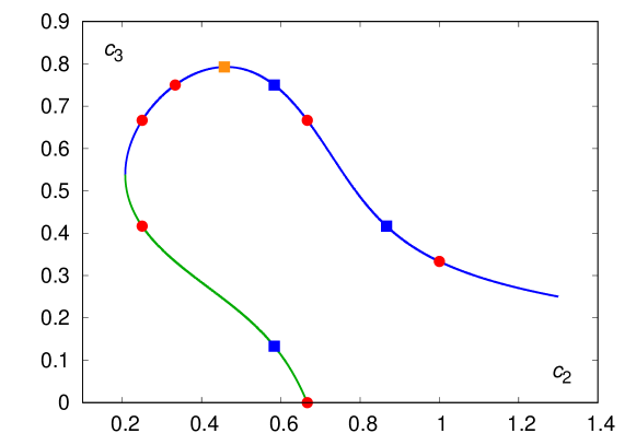
Figure 1: The two branches of solutions [12] of Eq. (32) shown as blue and green lines. The red circles show the solutions with rational coefficients found in [12] and the blue squares the solutions $(c_{2}=7/12,c_{3}=2/15)$, $(c_{2}=7/12,c_{3}=3/4)$ and $(c_{2}=13/15,c_{3}=5/12)$ that were missed in [12]. The orange square corresponds to the solution with minimal truncation error as defined in [18] which is used later as a basis of the BWRRK33 commutator-free Lie group method, see Sec. 5.

The $2N$-storage scheme introduces more constraints on the coefficients $a_{ij}$, $b_{i}$. However, they may be implicit: once the classical coefficients $a_{ij}$, $b_{i}$ are expressed in terms of the $2N$-storage coefficients $A_{i}$, $B_{i}$, one needs to search for a solution that satisfies only the original classical order conditions. For low-order schemes it may be useful to find the additional constraints explicitly, and we discuss a 3-stage third-order RK method in detail here to illustrate this point. In this case the coefficients no longer form a two-parameter family. The additional constraint can be imposed in different ways and a particular form used in Ref. [12] is

$$c_{3}^{2}(1-c_{2})+c_{3}\left(c_{2}^{2}+\frac{1}{2}c_{2}-1\right)+\left(\frac{1}{3}-\frac{1}{2}c_{2}\right)=0.$$ (32)

Choosing $c_{2}$ and then solving for $c_{3}$ from Eq. (32) allows one to reconstruct the coefficients $a_{ij}$, $b_{i}$ from (17)–(19), (13)–(16) and (6). Inverting the dependence (28), (31) produces the coefficients $A_{i}$, $B_{i}$ of the $2N$-storage scheme (20)–(24).

The two branches of solutions of $c_{3}$ as function of $c_{2}$ resulting from (32) are shown in Fig. 1. There is a reflection symmetry with respect to the $c_{2}+c_{3}=1$ axis which is apparent after a change of variables $c_{2}=x+y$, $c_{3}=1-x+y$.

3 Brief review of Lie group integrators with examples at third order

Let us now consider an equation of the form

$$\frac{dY}{dt}=A(Y)Y,$$ (33)

where $Y$ is a vector or a matrix. We use capital letters to emphasize that we now deal with objects that may not necessarily commute. Again, for simplicity we consider autonomous problems and extension to non-autonomous problems with $A(t,Y)$ is straightforward. Although the primary focus in this article is equations on Lie groups where $Y\in G$ and $A(Y)\in\mathfrak{g}$ where $G$ is a (matrix) Lie group and $\mathfrak{g}$ its Lie algebra, the discussion applies to structure-preserving integration of differential equations on manifolds in general [3]. The numerical examples in Sec. 5 include free rigid body rotation, where $Y$ is a three-dimensional vector of fixed length and the manifold is $S^{2}$, integration of the gradient flow on $SU(3)$ where $Y$ is an $SU(3)$ matrix and the manifold is obviously the $SU(3)$ group, van der Pol oscillator where $Y$ is a two-dimensional vector and the manifold is $R^{2}$ and more.

In the next subsections we review several existing Lie group integrators with examples at third order to define the building blocks necessary for the discussion in Sec. 4.

3.1 Crouch-Grossman methods

An update from $Y_{t}$ to $Y_{t+h}$ in the form of a classical RK method (3)–(5) is possible, however, even if $Y\in G$, the updated value of the form $Y+Const\cdot hA(Y)Y$ is no longer in the Lie group, in general. To maintain $Y$ on the manifold one needs to construct an update of the form $\exp(Const\cdot hA(Y))Y$. Then every stage of the RK-based method and the resulting $Y_{t+h}$ stays on the original manifold.

Crouch and Grossman [6] suggested an $s$-stage Lie group RK method of the following form:

$$Y_{i} = {\cal T}\left\{\prod_{j=1}^{i-1}\exp(ha_{ij}K_{j})\right\}Y_{t},$$ (34)

$$K_{i} = A(Y_{i}),$$ (35)

$$i = 1,\dots,s,$$ (36)

$$Y_{t+h} = {\cal T}\left\{\prod_{i=1}^{s}\exp(hb_{i}K_{i})\right\}Y_{t}.$$ (37)

Here ${\cal T}\prod$ represents a “time-ordered” product with a convention that an element with smaller value of the index is always located to the right. An explicit example clarifying this notation is given below in Eq. (39)–(45). In this case the number of $a_{ij}$, $b_{i}$ coefficients matches a classical $s$-stage RK method and can be represented with a Butcher table. The coefficients need to satisfy the classical order conditions and some additional constraints that result from non-commutativity. Ref. [6] considered methods up to order three and found that for a third-order method one has the following additional relation

$$\sum_{i}b_{i}^{2}c_{i}+2\sum_{i<j}b_{i}c_{i}b_{j}=\frac{1}{3}.$$ (38)

The order conditions for higher-order Lie group methods of this type were later derived in [19]. It turns out that a 3-stage third-order RK Lie group method is possible (since there are six coefficients and five constraints, giving a one-parameter family) and sets of coefficients satisfying (13)–(16) and (38) were given in Ref. [6]. Let us for the later convenience write the 3-stage third-order Crouch-Grossman RK method explicitly:

$$Y_{1} = Y_{t},$$ (39)

$$K_{1} = A(Y_{1}),$$ (40)

$$Y_{2} = \exp(ha_{21}K_{1})Y_{t},$$ (41)

$$K_{2} = A(Y_{2}),$$ (42)

$$Y_{3} = \exp(ha_{32}K_{2})\exp(ha_{31}K_{1})Y_{t},$$ (43)

$$K_{3} = A(Y_{3}),$$ (44)

$$Y_{t+h} = \exp(hb_{3}K_{3})\exp(hb_{2}K_{2})\exp(hb_{1}K_{1})Y_{t}.$$ (45)

From the computational perspective one can note the following. The method requires three evaluations of the right hand side of the differential equation, six exponentiations and storage for $K_{i}$ from all three stages, to be applied at the last step of the algorithm (45).

3.2 Munthe-Kaas methods

Another direction in constructing Lie group methods was taken by Munthe-Kaas in Refs. [7, 8, 9]. The most general approach worked out in Ref. [9] represents the solution $Y(t)$ as $Y(t)=\exp(U(t))Y(0)$ and constructs an algorithm for solving the equation for $U(t)$

$$\frac{dU}{dt}=d\exp_{U}^{-1}(A(Y(t))),$$ (46)

where the inverse derivative of the matrix exponential can be written as an expansion

$$d\exp_{U}^{-1}=\sum_{k=0}^{\infty}\frac{B_{k}}{k!}{\rm ad}_{U}^{k}.$$ (47)

$B_{k}$ are the Bernoulli numbers and the adjoint operator ${\rm ad}_{U}$ represents a mapping ${\rm ad}_{U}(V)=[U,V]=UV-VU$. The $k$-th power of ${\rm ad}_{U}$ is understood as an iterated application of this mapping:

$${\rm ad}_{U}^{0}(V) = V,$$ (48)

$${\rm ad}_{U}^{1}(V) = [U,V],$$ (49)

$${\rm ad}_{U}^{k}(V) = {\rm ad}_{U}({\rm ad}_{U}^{k-1}(V))=[U,[U,[\dots,[U,V]]]].$$ (50)

Let a truncated approximation of $d\exp_{U}^{-1}(V)$ be

$${\rm dexpinv}(U,V,p)=\sum_{k=0}^{p-1}\frac{B_{k}}{k!}{\rm ad}_{U}^{k}(V).$$ (52)

Then using the notation introduced in earlier sections, a Lie group $s$-stage order-$p$ RK method of Munthe-Kaas type has the following form:

$$U_{i} = h\sum_{j=1}^{i-1}a_{ij}\tilde{K}_{j},$$ (53)

$$Y_{i} = \exp(U_{i})Y_{t},$$ (54)

$$K_{i} = A(Y_{i}),$$ (55)

$$\tilde{K}_{i} = {\rm dexpinv}(U_{i},K_{i},p),$$ (56)

$$i = 1,\dots,s,$$ (57)

$$V = h\sum_{i=1}^{s}b_{i}\tilde{K}_{i},$$ (58)

$$Y_{t+h} = \exp(V)Y_{t}.$$ (59)

As shown in Ref. [9], if the coefficients $a_{ij}$, $b_{i}$ correspond to a classical RK method of order $p$ then the algorithm (53)–(59) with the truncation at $p-1$ in (52) is a Lie group integrator of order at least $p$. This procedure allows one to turn any classical $s$-stage order $p$ RK method into a Lie group integrator with the same number of stages and the same order at the expense of introducing commutators at every stage, Eq. (56). The number of commutators can be reduced as discussed in [20], and for later comparisons we write explicitly an earlier version [8] of the 3-stage third-order Lie group RK method of Munthe-Kaas type that requires only one commutator at the final stage:

$$Y_{1} = Y_{t},$$ (60)

$$K_{1} = A(Y_{1}),$$ (61)

$$Y_{2} = \exp(ha_{21}K_{1})Y_{t},$$ (62)

$$K_{2} = A(Y_{2}),$$ (63)

$$Y_{3} = \exp(h(a_{32}K_{2}+a_{31}K_{1}))Y_{t},$$ (64)

$$K_{3} = A(Y_{3}),$$ (65)

$$V = h\sum_{i=1}^{3}b_{i}K_{i},$$ (66)

$$\tilde{V} = V-\frac{h}{6}[K_{1},V],$$ (67)

$$Y_{t+h} = \exp(\tilde{V})Y_{t}.$$ (68)

Apart from the exponential action and the commutator in (67) this method resembles a classical RK method in that respect that one adds $K_{i}$ in a similar fashion as in a classical method and then exponentiates the result to produce $Y_{i}$ for the next stage. Here one needs three evaluations of the right hand side, three exponentiations and storage of $K_{i}$ from all three stages.

3.3 Celledoni-Marthinsen-Owren methods

Celledoni, Marthinsen and Owren in Ref. [10] considered an approach that generalizes Crouch-Grossman methods with the goal to avoid computation of commutators. Their idea is to introduce more than one exponential per stage of a RK method but allow for linear combinations of $K_{i}$ in the exponentials. An $s$-stage RK Lie group integrator can be written in the following form:

$$Y_{i} = {\cal T}\left\{\prod_{l=1}^{L_{i}}\exp\left(h\sum_{j=1}^{J_{il}}\alpha_{l;ij}K_{j}\right)\right\}Y_{t},$$ (69)

$$K_{i} = A(Y_{i}),$$ (70)

$$i = 1,\dots,s,$$ (71)

$$Y_{t+h} = {\cal T}\left\{\prod_{l=1}^{L}\exp\left(h\sum_{i=1}^{I_{l}}\beta_{l;i}K_{i}\right)\right\}Y_{t}.$$ (72)

The notation here is similar but not the same as in Ref. [10] to be more in line with the methods introduced earlier. Here $L_{i}$ is the number of exponentials used at stage $i$, $J_{il}$ is the upper bound on summation inside the $l$-th exponential at $i$-th stage, and, similarly, $L$ is the number of exponentials at the final stage and $I_{l}$ is the upper bound on summation inside the $l$-th exponential at the final stage. By introducing more parameters one has more room to satisfy the additional order conditions arising from non-commutativity at the expense of introducing more exponentials at each stage. The new coefficients $\alpha_{l;ij}$, $\beta_{l;i}$ are related to the coefficients of a classical RK method as [10]

$$\sum_{l=1}^{L_{i}}\alpha_{l;ij}=a_{ij},$$ (73)

$$\sum_{l=1}^{L}\beta_{l;i}=b_{i}.$$ (74)

The Crouch-Grossman method, Eqs. (39)–(45) is a subclass of the Celledoni-Marthinsen-Owren methods where $\alpha_{l;ij}=a_{ij}\delta_{lj}$ (and automatically $L_{i}=i-1$ for explicit methods).

Ref. [10] proceeded in a way that minimizes the number of exponentials and constructed schemes of third and fourth order that have the minimal number of exponentials and also reuse the exponentials at next stages. Here for comparison we write explicitly one of the solutions found in [10]:

$$Y_{1} = Y_{t},$$ (75)

$$K_{1} = A(Y_{1}),$$ (76)

$$Y_{2} = \exp(h\alpha_{1;21}K_{1})Y_{t},$$ (77)

$$K_{2} = A(Y_{2}),$$ (78)

$$Y_{3} = \exp(h(\alpha_{1;32}K_{2}+\alpha_{1;31}K_{1}))Y_{t},$$ (79)

$$K_{3} = A(Y_{3}),$$ (80)

$$Y_{t+h} = \exp(h(\beta_{2;3}K_{3}+\beta_{2;2}K_{2}+\beta_{2;1}K_{1}))\exp(h\beta_{1;1}K_{1})Y_{t}.$$ (81)

Requiring that $\beta_{1;1}=\alpha_{1;21}$ allows one to reuse $Y_{2}$ and calculate only one exponential at the last stage. This requirement also fixes these two coefficients to be equal to $1/3$ and the other coefficients then form a one-parameter family of solutions and their explicit form is given in Ref. [10]. Another branch of solutions reuses $Y_{3}$ and results in a method with the same computational requirements: three right hand side evaluations, three exponentiations and storage of $K_{i}$ from all stages and $Y_{2}$ or $Y_{3}$.

As one can see, at third order the Munthe-Kaas and Celledoni-Marthinsen-Owren methods have similar computational requirements, however, at fourth and higher order the situation is different: while Munthe-Kaas method can be constructed with the same number of exponentials as the number of stages in a classical RK method (with one exponential per stage), the Celledoni-Marthinsen-Owren methods require more exponentials (e.g., at least, five at fourth order).

4 A new class of commutator-free Lie group integrators

4.1 Construction of the integrator

Here we construct a new class of Lie group integrators. It can be considered as a subclass of Celledoni-Marthinsen-Owren methods, however, the construction proceeds differently and results in a family of solutions different from Ref. [10]. In particular this new scheme has different properties in terms of storage and exponentials reuse. At the same time, this new class can be considered as a subclass of the multirate infinitesimal step (MIS) methods used as exponential integrators [14], however, again, the family of solutions proposed here is different from the ones present in the literature.

Let us first construct a 3-stage third-order Lie group integrator and then comment on generalization of this scheme. Let us take the structure introduced in Eq. (69)–(72) and add the following requirements:

1. $L_{i}=i-1$ – as in the Crouch-Grossman method, stage $i$ has exactly $i-1$ exponentials.

2. $J_{il}=l$ – the number of terms within each exponential is equal to the index of that exponential in the sequence. With the time-ordering convention this means that the rightmost exponential has one term, the one to the left of it – two terms, and so on.

3. $L=s$ – at the final stage there is the maximum number, $s$ exponentials.

4. $I_{l}=l$ – the convention on the number of terms inside exponentials at the final stage is the same as in the previous stages.

Explicitly, a 3-stage algorithm (its order is not yet determined) is

$$Y_{1} = Y_{t},$$ (82)

$$K_{1} = A(Y_{1}),$$ (83)

$$Y_{2} = \exp(h\alpha_{1;21}K_{1})Y_{t},$$ (84)

$$K_{2} = A(Y_{2}),$$ (85)

$$Y_{3} = \exp(h(\alpha_{2;32}K_{2}+\alpha_{2;31}K_{1}))\exp(h\alpha_{1;31}K_{1})Y_{t},$$ (86)

$$K_{3} = A(Y_{3}),$$ (87)

$$Y_{t+h} = \exp(h(\beta_{3;3}K_{3}+\beta_{3;2}K_{2}+\beta_{3;1}K_{1}))$$ (88)

$$\times \exp(h(\beta_{2;2}K_{2}+\beta_{2;1}K_{1}))\exp(h\beta_{1;1}K_{1})Y_{t}.$$ (89)

This algorithm has six exponentials as the Crouch-Grossman method and also requires evaluating linear combinations of $K_{i}$ as in a classical RK method. There are 10 coefficients $\alpha_{l;ij}$, $\beta_{l;i}$ that are related to the classical RK coefficients via (73) and (74) and are subject to the four classical order conditions (13)–(16) and possibly other constraints arising from noncommutativity.

At first sight, there is nothing beneficial in this scheme as it requires more work than any other Lie group method introduced previously and therefore we apply another constraint:

1. The coefficients in the exponentials with the same number of terms are the same at all stages.

This means $\beta_{1;1}=\alpha_{1;31}=\alpha_{1;21}$, $\beta_{2;1}=\alpha_{2;31}$ and $\beta_{2;2}=\alpha_{2;32}$. This requirement allows one to reuse previous $Y_{i}$ at every stage and the scheme can be rewritten as

$$Y_{1} = Y_{t},$$ (90)

$$K_{1} = A(Y_{1}),$$ (91)

$$Y_{2} = \exp(h\alpha_{1;21}K_{1})Y_{1},$$ (92)

$$K_{2} = A(Y_{2}),$$ (93)

$$Y_{3} = \exp(h(\alpha_{2;32}K_{2}+\alpha_{2;31}K_{1}))Y_{2},$$ (94)

$$K_{3} = A(Y_{3}),$$ (95)

$$Y_{t+h} = \exp(h(\beta_{3;3}K_{3}+\beta_{3;2}K_{2}+\beta_{3;1}K_{1}))Y_{3}.$$ (96)

Now there are only three exponentials, the method reuses values of $Y_{i}$ from each previous stage and if the coefficients can be tuned that the scheme results in a third-order method, it can be on par with the methods of Sec. 3. There are now six independent coefficients, as in the classical 3-stage RK method and they are related to the coefficients of the classical method in a simple way:

$$\alpha_{1;21} = a_{21},$$ (97)

$$\alpha_{2;31} = a_{31}-a_{21},$$ (98)

$$\alpha_{2;32} = a_{32},$$ (99)

$$\beta_{3;1} = b_{1}-a_{31},$$ (100)

$$\beta_{3;2} = b_{2}-a_{32},$$ (101)

$$\beta_{3;3} = b_{3}.$$ (102)

Note that although a 3-stage third-order method is considered here as an example, the construction (90)–(96) is applicable in general. Eqs. (69)–(72) with the five requirements listed above essentially mean that in this format for a $s$-stage method each stage $i$ has only one exponential that contains a sum of all $K_{i}$ accumulated up to that stage that multiplies $Y_{i-1}$ from the previous stage:

$$Y_{0} \equiv Y_{t},$$ (103)

$$Y_{i} = \exp\left(h\sum_{j=1}^{i-1}\alpha_{i-1;ij}K_{j}\right)Y_{i-1},$$ (104)

$$K_{i} = A(Y_{i}),$$ (105)

$$i = 1,\dots,s,$$ (106)

$$Y_{t+h} = \exp\left(h\sum_{i=1}^{s}\beta_{s;i}K_{i}\right)Y_{s}.$$ (107)

However, as will be shown immediately below, a more compact format may be possible.

4.2 Order conditions for the new three-stage third-order Lie group method

By Taylor expanding the scheme (90)–(96) and comparing with the expansion of the exact solution one finds that the additional order conditions for this scheme to be globally of third order can be written as

$$b_{2}c_{2}^{2}+b_{3}c_{3}^{2}+(b_{2}c_{2}+b_{3}c_{3})(b_{1}+b_{2}+b_{3}+c_{3})+a_{32}c_{2}(c_{2}-b_{1}-b_{2}-b_{3})=1,$$ (108)

$$(b_{2}c_{2}+b_{3}c_{3})(b_{1}+b_{2}+b_{3}-c_{3})+a_{32}c_{2}(b_{1}+b_{2}+b_{3}-c_{2})=\frac{1}{3}.$$ (109)

With the use of the classical order conditions (13)–(16) one finds that these two conditions are not independent and result in a single condition:

$$a_{32}c_{2}(1-c_{2})=\frac{1}{6}(3c_{3}-1).$$ (110)

We can now multiply both sides by $b_{3}\neq 0$, use Eqs. (16) and (19) and rewrite (110) as a relation between $c_{2}$ and $c_{3}$:

$$c_{3}^{2}(1-c_{2})+c_{3}\left(c_{2}^{2}+\frac{1}{2}c_{2}-1\right)+\left(\frac{1}{3}-\frac{1}{2}c_{2}\right)=0.$$ (111)

Eq. (111) is exactly the same (!) as the relation (32) for the $2N$-storage scheme discussed in Sec. 2.2.

Let us summarize what has been achieved so far. We proposed a new format for a 3-stage commutator-free Lie group RK method (82)–(89) and, by requiring that it is of third order global accuracy, found that the order conditions on the classical RK coefficients of this method are the same as on the 3-stage third-order $2N$-storage scheme. Note, that the $2N$-storage schemes [12] were not intended as Lie group integrators and were designed as classical RK methods. The other way around, this means that although it was not imposed in (90)–(96), the relations between the coefficients are such that one does not need to store $K_{i}$ from all stages and this scheme can be rewritten in a $2N$-storage format by analogy with (20)–(24) as ($A_{1}=0$)

$$\Delta Y_{i} = A_{i}\Delta Y_{i-1}+hA(Y_{i-1}),$$ (112)

$$Y_{i} = \exp(B_{i}\Delta Y_{i})Y_{i-1},$$ (113)

$$i = 1,\dots,s,$$ (114)

$$Y_{0} \equiv Y_{t},$$ (115)

$$Y_{t+h} \equiv Y_{s},$$ (116)

where the coefficients $A_{i}$, $B_{i}$ are related to $a_{ij}$, $b_{i}$ in Eqs. (28) and (31).

4.3 Conjecture about higher order commutator-free Lie group integrators

The first main result of this paper derived in the previous section can be summarized as follows: The family of classical $2N$-storage 3-stage third-order RK schemes are also automatically third-order commutator-free Lie group integrators.

In fact, the third-order scheme, presented without derivation in the Appendix of Ref. [15] and used as a Lie group method for integration of $SU(3)$ gradient flow, belongs to the class of integrators proposed in Sec. 4.1 with a specific choice of coefficients from the one-parameter family of Eq. (111). This is discussed in more detail in the third numerical example in Sec. 5.3.

A natural question is: Are the $2N$-storage schemes at third order with more than three stages and at orders four and higher also commutator-free Lie group methods of the same order? While there is no analytic proof immediately available, the numerical evidence that is examined in Sec. 5 suggests that the answer to this question may be positive.

The second main result of this paper is the following conjecture: $2N$-storage $s$-stage classical RK schemes of order $p$ are also automatically commutator-free Lie group methods of the format proposed in Eqs. (112)–(116) of order $p$ for orders $p=3$, $4$, $5$ and possibly higher.

5 Numerical experiments

We now consider a few $2N$-storage classical RK schemes and apply them in several examples to provide support for the conjecture stated in Sec. 4.3.

First, we consider a 3-stage third-order family of $2N$-storage schemes for which it is proven in Sec. 4.2 that they are Lie group integrators of order $p=3$. We would like to choose a set of coefficients for which the truncation error is minimal in the sense of Ref. [18]. We need to emphasize the difference with the classical RK case. The 3-stage third-order classical RK scheme that has minimal truncation error found by Ralston [18] is not a $2N$-storage scheme and is not of third order if used as a Lie group integrator as defined in (90)–(96). However, one can follow the error minimization criteria of [18] with the additional constraint between $c_{2}$ and $c_{3}$, Eq. (111). The resulting set of classical RK coefficients was found by Williamson [12] and they turn out to be not rational. Unfortunately, Ref. [12] provided the coefficients with only five digits of accuracy which is not sufficient for the tests in this section. Therefore we improve on this by following the minimization procedure of [18] with the constraint (111) and the resulting set of coefficients is

$$a_{21} = \phantom{-}0.45737999756938819,$$ (117)

$$a_{31} = -0.13267640849031470,$$ (118)

$$a_{32} = \phantom{-}0.92529641092092174,$$ (119)

$$b_{1} = \phantom{-}0.19546562910003523,$$ (120)

$$b_{2} = \phantom{-}0.41072077622489378,$$ (121)

$$b_{3} = \phantom{-}0.39381359467507099.$$ (122)

By using (28), (31) they are transformed into the $2N$-storage format and used in the commutator-free Lie group method, Eqs. (112)–(116). We use this scheme, called BWRRK33, in the examples below, and we also tested it with the nine sets of rational coefficients shown in Fig. 1, six of which were found in [12].

Next, we also consider thirteen $2N$-storage schemes available in the literature. The nomenclature used here is the following. Letters “RK” in the middle indicate that this is a classical RK method, the letters in front abbreviate the names of the authors or the name given to the scheme in the original article, the last digit is the order of the method, the digits in front of it represent the number of stages and the additional letters after “RK” possible notation from the original article to distinguish integrators with different properties. The list of all fourteen $2N$-storage schemes tested in the examples is given in Table 1.

Table 1: Method 1, BWRRK33 is proven to be a third-order commutator-free Lie group method in Sec. 4.2. Methods 2–14 are classical $2N$-storage RK methods available in the literature used to test the conjecture formulated in Sec. 4.3. We note that for the BWRRK33 method we also ran numerical tests with the rational coefficients shown in Fig. 1 and for the CKRK54 method we ran tests with all four sets of coefficients found in Ref. [21]. For presenting results we, however, chose only one, recommended set of coefficients from [21]. Similarly, there are four sets of coefficients for the BPRKO73 method in Ref. [22] which we tested, but for presenting the results we chose the set called ORK37-6 in Ref. [22]. Note also that BBBRKNL64 is called RK46-NL in Ref. [23].

	Name	Stages	Order	Reference
1	BWRRK33	3	3	Here, [12], [18]
2	BPRKO73	7	3	[22]
3	TSRKC73	7	3	[24]
4	CKRK54	5	4	[21]
5	SHRK64	6	4	[25]
6	BBBRKNL64	6	4	[23]
7	HALERK64	6	4	[26]
8	HALERK74	7	4	[26]
9	TSRKC84	8	4	[24]
10	TSRKF84	8	4	[24]
11	NDBRK124	12	4	[27]
12	NDBRK134	13	4	[27]
13	NDBRK144	14	4	[27]
14	YRK135	13	5	[28]

It is important to stress that while we proved that the BWRRK33 scheme is a commutator-free Lie group integrator with global accuracy of order $p=3$, Sec. 4.2, none of the other schemes in Table 1 were originally designed as Lie group integrators. They are $2N$-storage classical RK methods which were designed to have specific properties such as increased stability regions, low dissipation, etc. If one attempts to use an order $p$ arbitrary classical RK scheme whose coefficients satisfy only the classical RK constraints as a Lie group integrator, the order of accuracy is less than $p$, and as numerical experiments show, typically second order at best. Thus, the thirteen $2N$-storage schemes (in addition to BWRRK33) collected in Table 1 are a perfect test of the conjecture in Sec. 4.3 if they maintain the same order of accuracy when used as commutator-free Lie group methods in the sense of Eqs. (112)–(116).

Also, while it is not yet proven (or refuted) that any $2N$-storage method of order $p$ is also a commutator-free Lie group integrator of order $p$, for a given set of numerical values of the coefficients the order conditions can be algorithmically checked by using B-series [29]. All the methods of Table 1 were independently checked by Knoth with the software available at [29] and they indeed fulfill the order conditions corresponding to the order shown in the table when used as Lie group integrators.

For numerical experiments in our code we also implemented integrators of other types, namely, Crouch-Grossman method of order $p=3$ [6], Munthe-Kaas methods of order $p=3$, $4$, $5$, $8$ [9], Celledoni-Marthinsen-Owren methods [10] of order $p=3$ and $4$. In the tests below as a reference we use the following Lie group integrators of Munthe-Kaas (RKMK) type:

• 3-stage third-order with Ralston coefficients,

• 4-stage fourth-order with Ralston coefficients,

• 6-stage fifth-order with Butcher coefficients.

5.1 Example 1: Free rigid body rotation

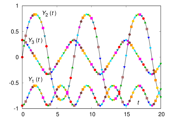
Figure 2: Comparison of the exact solution for the three components of the angular momentum (see text), shown as the gray lines, with the results produced by the fourteen integrators listed in Table 1. If plotted as lines, all results are indistinguishable from the exact solution. Therefore we plot the results from different integrators as symbols of different shape and color skipping 140 steps in the sequence and starting to plot the first integrator at a shift of 0 steps, second at a shift of 10 steps and so on.

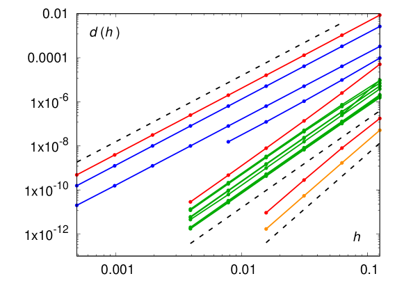
Figure 3: Distance from the reference (exact) solution $d(h)$ for various integrators as function of step size $h$ shown in a log-log plot for the rigid body problem, Eq. (125). The red lines represent the three integrators of Munthe-Kaas type of order $p=3$, $4$ and $5$. The three blue lines represent the three integrators of order $p=3$ from Table 1, the ten green lines the ten integrators of order $p=4$ and the orange line one integrator of order $p=5$ from the same table. For the $p=4$ integrators the minimum step size shown is $1/256$ and for $p=5$ $1/64$ since when $d(h)$ becomes comparable to $10^{-13}$ the roundoff errors prevent correct scaling behavior. The black dashed lines are shown to guide the eye and represent from top to bottom $h^{3}$, $h^{4}$ and $h^{5}$, respectively.

As a first numerical example we consider rotation of a free rigid body with the center of mass fixed at the origin. This example was used in Ref. [10, 30]. In this case, $Y$ is a three-dimensional vector of angular momentum and the Euler equation is

$$\frac{dY}{dt}=Y\times I^{-1}Y,$$ (123)

where $I$ is the inertia tensor. By using the hat map $\hat{\,}{\,}$: $R^{3}\to\mathfrak{so}(3)$ defined as

$$V=\left(\begin{array}[]{c}v_{1}\\ v_{2}\\ v_{3}\\ \end{array}\right)\to\hat{V}=\left(\begin{array}[]{rrr}0&-v_{3}&v_{2}\\ v_{3}&0&-v_{1}\\ -v_{2}&v_{1}&0\end{array}\right)$$ (124)

the Euler equation can be rewritten in the form (33)

$$\frac{dY}{dt}=-\widehat{I^{-1}Y}Y$$ (125)

with $A(Y)\equiv-\widehat{I^{-1}Y}$. For the tensor of inertia we take the same value $I=diag(7/8,5/8,1/4)$ as in [10] but choose a different initial condition $Y(0)=(-\sqrt{8}/3,0,1/3)$. Such an initial condition matches the simplifying assumptions of [31] where the exact solution is given in terms of Jacobi’s elliptic functions. First, to check the implementation of the integrators in our code, we compare the trajectory integrated from $t=0$ to $t=20$ with the time step $h=0.025$ with all fourteen integrators of Table 1 with the exact solution. The result is shown in Fig. 2.

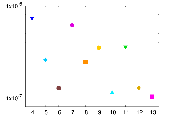
Figure 4: Distance from the reference solution $d(h)$ at $h=1/16$ for all fourth-order integrators from Table 1 for the rigid body problem, Eq. (125). The symbols and colors are the same as in Fig. 2 and the numbers on the horizontal axis correspond to the numbering in Table 1.

Next, to study the order of the methods we integrate the equation of motion from $t=0$ to $t=3$ by using the step size $h=1/2^{n}$ where $n=3,\dots,11$. Let $Y(t=3,h)$ be the solution evaluated at a particular step size $h$ and $Y_{ref}(t=3)$ the exact solution [31]. We define a distance metric as

$$d(h)=|Y(t=3,h)-Y_{ref}(t=3)|,$$ (126)

where $|\dots|$ is the usual Euclidean vector norm. If an integrator has the global order of accuracy $p$ then one expects $d(h)\sim h^{p}$. The results for $d(h)$ for the fourteen integrators of Table 1 and the three reference integrators are shown in Fig. 3. We note that the BPRKO73, SHRK64 and BBBRKNL64 integrators are somewhat problematic since their coefficients are given with less than full double precision accuracy. Their scaling breaks down when $d(h)$ reaches about $10^{-8}$, $10^{-7}$ and $10^{-11}$, respectively. Therefore we plot $d(h)$ approximately down to those limits for those integrators.

As one can observe from Fig. 3, the $2N$-storage classical RK schemes provide the same global order of accuracy when used as manifold integrators of a new format defined in Eqs. (112)–(116), supporting the conjecture stated in Sec. 4.3.

Some of the RK methods of fourth order shown in Fig. 3 as green lines have comparable global errors and their lines are hard to distinguish on the scale of the plot. In Fig. 4 we show the distance from the exact solution $d(h)$ at $h=1/16$ for each method of order 4 from Table 1. For instance, methods 4 and 7, 5 and 8, 9 and 11, and 6, 10, 12 and 13 produce similar $d(h)$ in this example. Similar features are observed in the other examples considered below but which particular methods produce close results depends on the differential equation.

A simple Matlab script illustrating the usage of BWRRK33, TSRKF84 and YRK135 as Lie group integrators for this example is given in A.

5.2 Example 2: $SO(5)$ from Ref. [9]

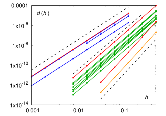
Figure 5: Distance from the reference solution $d(h)$ for various integrators as function of step size $h$ shown in a log-log plot for the $SO(5)$ manifold in example 2, Eq. (127). As in Fig. 3, the red lines represent the three integrators of Munthe-Kaas type of order $p=3$, $4$ and $5$. The three blue lines represent the three integrators of order $p=3$ from Table 1, the ten green lines the ten integrators of order $p=4$ and the orange line one integrator of order $p=5$ from the same table. For the $p=4$ integrators the minimum step size shown is $1/128$ and for $p=5$ $1/32$ since when $d(h)$ becomes comparable to $10^{-13}$ the roundoff errors prevent correct scaling behavior. The black dashed lines are shown to guide the eye and represent from top to bottom $h^{3}$, $h^{4}$ and $h^{5}$, respectively.

Our second numerical example is the one used in [9], where $Y$ is an $SO(5)$ matrix and the skew-symmetric matrix $A(Y)$ on the right hand side in Matlab notation is

$$A(Y)={\rm diag}({\rm diag}(Y,+1),+1)-{\rm diag}({\rm diag}(Y,+1),-1).$$ (127)

The inital condition $Y(0)=Y_{0}$ is produced randomly with

$${\rm rand}(\mbox{`seed'},0);\,\,\,\,\,\,\,[Y_{0},R]={\rm qr}({\rm rand}(5,5)).$$ (128)

We integrate the equation of motion from $t=0$ to $t=5$ using the step size $h=1/2^{n}$, $n=1,\dots,10$. As the reference solution at time $t=5$ $Y_{ref}(t=5)$ we use the solution produced by the package DiffMan [32] with the RKMK method of order $p=6$ butcher6 with the step size $h=1/512$. As in the previous example we define the distance from the reference solution

$$d(h)=|Y(t=5,h)-Y_{ref}(t=5)|,$$ (129)

where $|\dots|$ is the matrix 2-norm, evaluated in Matlab as norm. The results for $d(h)$ are shown in Fig. 5. The integrators again show expected scaling supporting the conjecture stated in Sec. 4.3.

5.3 Example 3: $SU(3)$ gradient flow

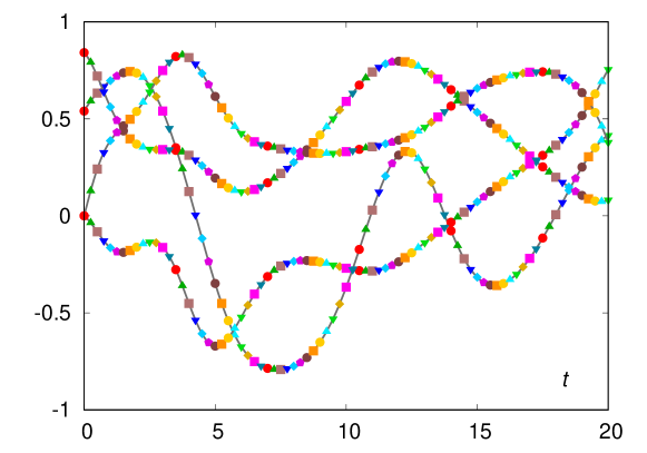
Figure 6: Comparison of the reference solution (see text) for the real and imaginary parts of the $SU(3)$ matrix elements $Y_{11}(t)$, $Y_{12}(t)$, shown as the four gray lines, with the results produced by the fourteen integrators listed in Table 1. If plotted as lines, all results are indistinguishable from the exact solution. Therefore we plot the results from different integrators as symbols of different shape and color skipping 140 steps in the sequence and starting to plot the first integrator at a shift of 0 steps, second at a shift of 10 steps and so on.

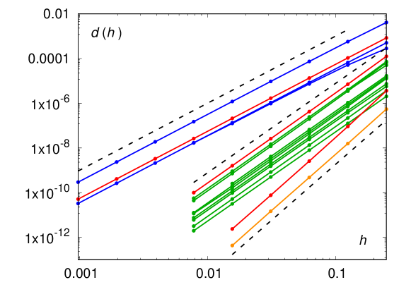
Figure 7: Distance from the reference solution $d(h)$ for various integrators as function of step size $h$ shown in a log-log plot for the $SU(3)$ manifold in example 3, Eq. (130). As in Fig. 3, the red lines represent the three integrators of Munthe-Kaas type of order $p=3$, $4$ and $5$. The three blue lines represent the three integrators of order $p=3$ from Table 1, the ten green lines the ten integrators of order $p=4$ and the orange line one integrator of order $p=5$ from the same table. For the $p=4$ integrators the minimum step size shown is $1/128$ and for $p=5$ $1/64$ since when $d(h)$ becomes comparable to $10^{-13}$ the roundoff errors prevent correct scaling behavior. The black dashed lines are shown to guide the eye and represent from top to bottom $h^{3}$, $h^{4}$ and $h^{5}$, respectively.

As a third example we consider an application that is relevant for a non-perturbative approach to quantum field theory called lattice gauge theory. In this case the degrees of freedom are $SU(3)$ group elements that reside on links of a four-dimensional space-time grid and the interactions in the system are encoded in traces of products of the $SU(3)$ matrices taken along closed paths on the grid. Lüscher in Ref. [15] introduced a diffusion-like procedure that suppresses short-wavelength fluctuations in the system. This procedure leads to the following equation on the $SU(3)$ manifold:

$$\frac{dY}{dt}=-{\cal P}\left\{HY\right\}Y,$$ (130)

where $Y\in SU(3)$ and $H\in GL(3,C)$ encodes the interactions with the neighboring degrees of freedom on the grid. Here for numerical experiments we consider a single degree of freedom $Y$ in the presence of a fixed background $H$. The projection

$${\cal P}\left\{M\right\}=\frac{1}{2}\left(M-M^{\dagger}\right)-\frac{1}{6}{\rm Tr}\left(M-M^{\dagger}\right)$$ (131)

produces an element of the algebra $\mathfrak{su}(3)$ and the right hand side of Eq. (33) in this case is

$$A(Y)=-{\cal P}\left\{HY\right\},$$ (132)

where $H$ is constant. We choose $H$ as a random $3\times 3$ complex matrix and take a diagonal initial condition $Y(t=0)=diag(e^{i},e^{i},e^{-2i})$. Here again, to test the implementation of the integrators, we compare the trajectory integrated with the fourteen methods of Table 1 with the solution obtained with DiffMan with the RKMK integrator butcher6 at step size $h=1/512$. The results for the real and imaginary parts of the matrix elements $Y_{11}(t)$ and $Y_{12}(t)$ are shown in Fig. 6.

For the scaling study we use the same random matrix $H$ and the same initial condition. The trajectory is integrated from $t=0$ to $t=10$ with $h=1/2^{n}$, $n=1,\dots,10$ and as before we use the 2-norm as a measure of deviation from the reference solution

$$d(h)=|Y(t=10,h)-Y_{ref}(t=10)|.$$ (133)

The results for $d(h)$ are shown in Fig. 7.

The integrator suggested by Lüscher in the Appendix of Ref. [15] for integrating this system, Eq. (130) is, in fact, a 3-stage third-order $2N$-storage integrator of the family (111) for which we have proven in Sec. 4.2 that all integrators of this family are third-order Lie group methods. The choice of the classical coefficients equivalent to the scheme in [15] is

$$a_{21} = \phantom{-}\frac{1}{4},$$ (134)

$$a_{31} = -\frac{2}{9},$$ (135)

$$a_{32} = \phantom{-}\frac{8}{9},$$ (136)

$$b_{1} = \phantom{-}\frac{1}{4},$$ (137)

$$b_{2} = \phantom{-}0,$$ (138)

$$b_{3} = \phantom{-}\frac{3}{4}.$$ (139)

Although the integrator in Ref. [15] was not written in the $2N$-storage format, it was realized there that this scheme can be used as a low-storage scheme, independently of the earlier work [12]. Applications to lattice gauge theory is a case where low-storage schemes are especially attractive, since realistic systems include grids of the size up to $96^{3}\times 192$ [33] which translates to about $1.2\times 10^{10}$ double precision numbers to be stored on a (super)computer just to represent the system. While using a $2N$-storage scheme requires twice that amount, an equivalent 3-stage third-order RKMK method requires four times this amount, with further increasing requirements for higher order schemes. Since the conjecture about higher than order $p=3$ $2N$-storage classical RK methods holds true numerically for the $SU(3)$ case, as illustrated in Fig. 7, this opens a possibility of constructing higher order Lie group $2N$-storage methods for applications in lattice gauge theory.

5.4 Example 4: Van der Pol oscillator

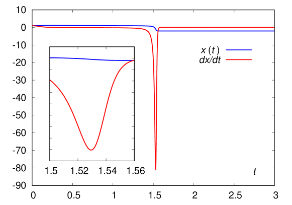
Figure 8: The dependence of the coordinate $x(t)$ (blue) and the velocity $\dot{x}(t)$ (red) on time for the van der Pol system, Eq. (140). This solution is produced with the BWRRK33 integrator with step size $h=0.001$. The other integrators produce results indistinguishable on the scale of the figure and are not shown. The inset magnifies the horizontal scale in the vicinity of the “needle”.

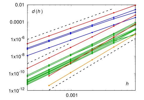
Figure 9: Distance from the reference solution $d(h)$ for various integrators as function of step size $h$ shown in a log-log plot for the van der Pol oscillator in example 4, Eq. (140). As in Fig. 3, the red lines represent the three integrators of Munthe-Kaas type of order $p=3$, $4$ and $5$. The three blue lines represent the three integrators of order $p=3$ from Table 1, the ten green lines the ten integrators of order $p=4$ and the orange line one integrator of order $p=5$ from the same table. For the $p=5$ integrators the minimum step size shown is $1/2048$ since when $d(h)$ becomes comparable to $10^{-13}$ the roundoff errors prevent correct scaling behavior. The black dashed lines are shown to guide the eye and represent from top to bottom $h^{3}$, $h^{4}$ and $h^{5}$, respectively.

The van der Pol equation

$$\frac{d^{2}x}{dt^{2}}-\mu(1-x^{2})\frac{dx}{dt}+x=0$$ (140)

has also been used as a test case in the literature on Lie group methods [30]. In this case, a Lie group method is used as an exponential integrator that may handle stiff systems better than classical RK schemes. Eq. (140) can be rewritten in a vector form

$$\frac{d}{dt}\left(\begin{array}[]{c}x\\ \dot{x}\end{array}\right)=\left(\begin{array}[]{rc}0&1\\ -1&\mu(1-x^{2})\end{array}\right)\left(\begin{array}[]{c}x\\ \dot{x}\end{array}\right)$$ (141)

where we can identify $Y$ as a two-dimensional vector and $A(Y)\in GL(2,R)$. As in Ref. [30] we choose $\mu=60$ and the initial condition

$$Y(0)=\left(\begin{array}[]{c}1\\ 1\end{array}\right).$$ (142)

At such a large value of $\mu$ the system is stiff as shown in Fig. 8 and the “needle” occurs approximately at $t=1.53$.

We integrate the system from $t=0$ to $t=2$, i.e. past the “needle”, with step size $h=1/2^{n}$, $n=7,\dots,12$. As a reference solution $Y_{ref}(t=2)$ we use the result from the DiffMan package with the RKMK integrator butcher6 at step size $h=1/4096$ and define the distance from the reference solution $d(h)$ the same way as in the Example 1 in Sec. 5.1. The results for $d(h)$ for various $2N$-storage schemes of Table 1 are shown in Fig. 9.

Notice that given the stiffness of the system, we use, in general, a range of smaller step sizes than in the other examples, but all the integrators do show the scaling expected from the conjecture in Sec. 4.3.

5.5 Example 5: Non-autonomous problem in $SO(3)$

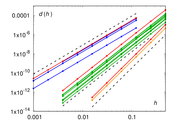
Figure 10: Distance from the reference solution $d(h)$ for various integrators as function of step size $h$ shown in a log-log plot for the $SO(3)$ matrix $Y$ in example 5 (non-autonomous problem), Eq. (143). As in Fig. 3, the red lines represent the three integrators of Munthe-Kaas type of order $p=3$, $4$ and $5$. The three blue lines represent the three integrators of order $p=3$ from Table 1, the ten green lines the ten integrators of order $p=4$ and the orange line one integrator of order $p=5$ from the same table. For the $p=4$ integrators the minimum step size shown is $1/256$ and for $p=5$ $1/64$ since when $d(h)$ becomes comparable to $10^{-13}$ the roundoff errors prevent correct scaling behavior. The black dashed lines are shown to guide the eye and represent from top to bottom $h^{3}$, $h^{4}$ and $h^{5}$, respectively.

As the final example we consider a non-autonomous problem which is included as one of the examples in DiffMan [32]: $Y\in SO(3)$ and

$$A(t,Y)=\left(\begin{array}[]{rrr}0&t\phantom{{}^{2}}&1\phantom{{}^{2}}\\ -t&0\phantom{{}^{2}}&-t^{2}\\ -1&t^{2}&0\phantom{{}^{2}}\end{array}\right)\in\mathfrak{so}(3).$$ (143)

This test is different from the previous ones since the coefficients $c_{i}$, Eq. (6), now enter the game and we investigate if that may lead to a breakdown of the conjecture of Sec. 4.3. We choose a unit matrix as the initial condition, as in DiffMan, and integrate the trajectory from $t=0$ to $t=1$ with step sizes $h=1/2^{n}$, $n=1,\dots,10$. As the reference solution we take the result from DiffMan integrated with butcher6 with $h=1/1024$. The distance from the reference solution $d(h)$ is defined the same way as in examples 2, Sec. 5.2 and 3, Sec. 5.3. The results for $d(h)$ for the methods of Table 1 is shown in Fig. 10. As can be observed from the figure, the integrators again show the expected scaling.

6 Conclusions

We have shown in Sec. 4.2 that 3-stage third-order classical $2N$-storage Runge-Kutta methods of Ref. [12] are also third-order commutator-free Lie group methods, since the coefficients satisfy the same order conditions in both cases: four classical ones and an additional one arising either from writing the scheme in $2N$-storage format [12] or constructing a commutator-free Lie group integrator in a specific format proposed in Eqs. (82)–(89) that automatically leads to Eqs. (90)–(96).

Given this similarity, we conjectured in Sec. 4.3 that this observation holds also for third-order $2N$-storage classical RK methods with more than three stages and for methods of order four and five. In Sec. 5 we considered five different numerical examples and studied how the global error of the $2N$-storage classical RK methods available in the literature [21, 22, 23, 24, 25, 26, 27, 28] scales with the step size when the schemes are used as commutator-free Lie group methods of the $2N$-storage format proposed in Eqs. (112)–(116). We found that in all test cases numerical evidence supports the conjecture.

As a next step, it is obviously desirable to find an analytic proof of the conjecture of Sec. 4.3. In the meantime, one can check the order conditions for a Lie group integrator based on a given $2N$-storage coefficients scheme with the methods of Ref. [29] or determine what order is achieved numerically as in the examples presented in Sec. 5.

If the conjecture is proven to be correct, there are two possible benefits of the proposed low-storage commutator-free Lie group integrators. First, in large-scale calculations one can significantly reduce memory requirements compared to the available Lie group methods (both, commutator-free and with commutators) and also reuse the exponentials at every step of the calculation which leads to the requirement of evaluating exactly $s$ exponentials for a $s$-stage method. Second, it may be easier to develop new schemes of this type for differential equations on manifolds in a way it has been done for the classical $2N$-storage methods. Once the scheme is written in a $2N$-storage format, Eqs. (112)–(116), one needs to find the coefficients of the $2N$-storage scheme from satisfying only classical Runge-Kutta order conditions. The property that the scheme is a $2N$-storage scheme will automatically (again, if the conjecture is true) satisfy all the additional constraints arising from non-commutativity.

Acknowledgements. I thank Andrea Shindler for careful reading and comments on the manuscript and Oswald Knoth for bringing my attention to Ref. [13, 14], comments on the manuscript and, most importantly, for independently checking the order conditions for all coefficient schemes of Table 1 (as Lie group integrators of the form (112)–(116)) with his software available at [29] and explaining me the theory and algorithmic details behind that software. This work was in part supported by the U.S. National Science Foundation under award PHY-1812332.

Appendix A Matlab code

To illustrate the usage of the $2N$-storage schemes as commutator-free Lie group integrators we present below a Matlab script that generates a scaling plot similar to Fig. 3 using the integrators BWRRK33, TSRKF84 and YRK135 from Table 1.

%%%%%%%%%%%%%%%%%%%%%%%%%%%%%%%%
% main function in the script:
% get scaling with step size
% by comparing to exact solution
%%%%%%%%%%%%%%%%%%%%%%%%%%%%%%%%
function lie_integrate

format long;

global I;

% initial condition
% second component is 0 to match
% simplifying assumptions of exact solution
% in Marsden, Ratiu, Introduction to Mechanics and Symmetry
y0 = [ -sqrt(8)/3; 0; 1/3 ];

% moment of intertia, same as in
% Celledoni, Marthinsen, Owren
% Future Generation Computer Systems, 19 (2003) 341-352
I1 = 7/8;
I2 = 5/8;
I3 = 1/4;
I = diag( [ I1 I2 I3 ] );

% integration parameters
T0 = 0;
T = 3;

% set array with time steps
array_dt = ...
[ 1/2048 1/1024 1/512 1/256 1/128 1/64 1/32 1/16 1/8 1/4 1/2 ];
Ndt = length( array_dt );

% number of integrators
Nint = 3;

% storage
error_dt = zeros( Ndt, Nint );
sol = zeros( 3, Ndt, Nint);

% coefficients for low-storage integrators
% 3-stage third-order BWRRK33
Nstages_3 = 3;
A_3 = [ 0 ...
       -0.637694471842202 ...
       -1.306647717737108 ];
B_3 = [ 0.457379997569388 ...
        0.925296410920922 ...
        0.393813594675071 ];
C_3 = [ 0 ...
        0.457379997569388 ...
        0.792620002430607 ];
% 8-stage fourth-order TSRKF84 of
% Toulorge, Desmet, J. Comp. Phys. 231 (2012) 2067-2091
Nstages_4 = 8;
A_4 = [ 0 ...
       -0.5534431294501569 ...
        0.01065987570203490 ...
       -0.5515812888932000 ...
       -1.885790377558741 ...
       -5.701295742793264 ...
        2.113903965664793 ...
       -0.5339578826675280 ];
B_4 = [ 0.08037936882736950 ...
        0.5388497458569843 ...
        0.01974974409031960 ...
        0.09911841297339970 ...
        0.7466920411064123 ...
        1.679584245618894 ...
        0.2433728067008188 ...
        0.1422730459001373 ];
C_4 = [ 0 ...
        0.08037936882736950 ...
        0.3210064250338430 ...
        0.3408501826604660 ...
        0.3850364824285470 ...
        0.5040052477534100 ...
        0.6578977561168540 ...
        0.9484087623348481 ];
% 13-stage fifth-order YRK135 of
% Yan, Chin. J. Chem. Phys 30 (2017) 277-286
Nstages_5 = 13;
A_5 = [ 0 ...
       -0.33672143119427413 ...
       -1.2018205782908164 ...
       -2.6261919625495068 ...
       -1.5418507843260567 ...
       -0.2845614242371758 ...
       -0.1700096844304301 ...
       -1.0839412680446804 ...
       -11.61787957751822 ...
       -4.5205208057464192 ...
       -35.86177355832474 ...
       -0.000021340899996007288 ...
       -0.066311516687861348 ];
B_5 = [ 0.069632640247059393 ...
        0.088918462778092020 ...
        1.0461490123426779 ...
        0.42761794305080487 ...
        0.20975844551667144 ...
       -0.11457151862012136 ...
       -0.01392019988507068 ...
        4.0330655626956709 ...
        0.35106846752457162 ...
       -0.16066651367556576 ...
       -0.0058633163225038929 ...
        0.077296133865151863 ...
        0.054301254676908338 ];
C_5 = [ 0 ...
        0.069632640247059393 ...
        0.12861035097891748 ...
        0.34083022189561149 ...
        0.54063706308495402 ...
        0.59927749518613931 ...
        0.49382042519248519 ...
        0.48207852767699775 ...
        0.82762865209834452 ...
        0.82923953914857933 ...
        0.67190565554748019 ...
        0.87194975193167848 ...
        0.94930216564503562 ];


% parameters for exact solution
I1y0 = (I^-1) * y0;
h = 1/2 * ( y0.’*I1y0 );
y02 = y0.’*y0;
a = y02 / (2*h);
b = 2*h / sqrt(y02);
alpha = sqrt( a*I2*(a-I3)/(I2-I3) ) * b;
beta = sqrt( a*I2*(I1-a)/(I1-I2) ) * b;
mu = sqrt( a*(I1-a)*(I2-I3)/(I1*I2*I3) ) * b;
k = sqrt( (I1-I2)*(a-I3)/(I1-a)/(I2-I3) );
delta = sqrt( I3*(I1-a)*a/(I1-I3) ) * b;
gamma = sqrt( I1*(a-I3)*a/(I1-I3) ) * b;

% exact solution at T
snmt = jacobiSN( mu*T, k^2 );
cnmt = jacobiCN( mu*T, k^2 );
dnmt = jacobiDN( mu*T, k^2 );
y_exact = [ -gamma * cnmt; alpha * snmt; delta * dnmt ];


% loop over step sizes
for idt = 1:Ndt

 % integrate with current step size
 for iint=1:Nint
  dt = array_dt(idt);
  if iint==1
   sol( :, idt, iint ) = ...
   integrate( T0, T, dt, y0, @rhs_f, Nstages_3, A_3, B_3, C_3 );
  elseif iint==2
   sol( :, idt, iint ) = ...
   integrate( T0, T, dt, y0, @rhs_f, Nstages_4, A_4, B_4, C_4 );
  elseif iint==3
   sol( :, idt, iint ) = ...
   integrate( T0, T, dt, y0, @rhs_f, Nstages_5, A_5, B_5, C_5 );
  end

  % get error
  error_dt( idt, iint ) = norm( sol( :, idt, iint ) - y_exact );
 end

end

% plot
for iint=1:Nint
 if iint==1
  cc = [1 0 0];
  xaxis = array_dt;
  yaxis = error_dt( :, iint );
 elseif iint==2
  cc = [0 0.7 0];
  xaxis = array_dt( 3:Ndt );
  yaxis = error_dt( 3:Ndt, iint );
 elseif iint==3
  cc = [0 0 1];
  xaxis = array_dt( 5:Ndt );
  yaxis = error_dt( 5:Ndt, iint );
 end
 loglog( xaxis, yaxis, ’Color’, cc, ’LineWidth’, 3 );
 if iint==1
  hold on
 end
end
hold off

end

%%%%%%%%%%%%%%%%%%%%%%%%%%%%
% right hand side function
% t - current time
% y - current function value
%%%%%%%%%%%%%%%%%%%%%%%%%%%%
function r = rhs_f( t, y )

 global I;

 I1y = (I^-1) * y;
 r = zeros(3,3);
 r(1,2) =  I1y(3);
 r(2,1) = -I1y(3);
 r(1,3) = -I1y(2);
 r(3,1) =  I1y(2);
 r(2,3) =  I1y(1);
 r(3,2) = -I1y(1);

end

%%%%%%%%%%%%%%%%%%%%%%%%%%%%%%%%%%%%%%%%%%%%%%%%%%
% low-storage commutator-free Lie group integrator
% T0 - initial time
% T - final time
% dt - step size
% Y0 - initial function value
% rhs - function to evaluate right hand side
% Ns - number of stages of the integrator
% A, B, C - coefficients in 2N-storage format
% Note: A(1)=0 is required
% result - function value at time T Y(t=T)
%%%%%%%%%%%%%%%%%%%%%%%%%%%%%%%%%%%%%%%%%%%%%%%%%%
function result = integrate( T0, T, dt, Y0, rhs, Ns, A, B, C )

 % current time
 Tcur = T0;
 % initial function value
 Y = Y0;
 dY = 0;

 while Tcur < T
  if dt > T-Tcur
   dt = T - Tcur;
  end

  for k=1:Ns
   dY = A(k)*dY + dt*rhs( Tcur + C(k)*dt, Y );
   Y = expm( B(k)*dY )*Y;
  end

  % set values for next iteration
  Tcur = Tcur + dt;
 end

 result = Y;

end

References

- [1] J. Butcher, Numerical Methods for Ordinary Differential Equations, 3rd Edition, Wiley, 2016.
- [2] E. Hairer, S. Nørsett, G. Wanner, Solving Ordinary Differential Equations I Nonstiff problems, 2nd Edition, Springer, Berlin, 2000.
- [3] E. Hairer, C. Lubich, G. Wanner, Geometric Numerical Integration: Structure-Preserving Algorithms for Ordinary Differential Equations; 2nd ed., Springer, Dordrecht, 2006. doi:10.1007/3-540-30666-8.
- [4] S. H. Christiansen, H. Z. Munthe-Kaas, B. Owren, Topics in structure-preserving discretization, Acta Numerica 20 (2011) 1–119. doi:10.1017/S096249291100002X.
- [5] E. Celledoni, H. Marthinsen, B. Owren, An introduction to Lie group integrators – basics, new developments and applications, Journal of Computational Physics 257 (2014) 1040 – 1061, physics-compatible numerical methods. doi:https://doi.org/10.1016/j.jcp.2012.12.031.
- [6] P. E. Crouch, R. Grossman, Numerical integration of ordinary differential equations on manifolds, Journal of Nonlinear Science 3 (1) (1993) 1–33. doi:10.1007/BF02429858.
- [7] H. Munthe-Kaas, Lie-Butcher theory for Runge-Kutta methods, BIT Numerical Mathematics 35 (4) (1995) 572–587. doi:10.1007/BF01739828.
- [8] H. Munthe-Kaas, Runge-Kutta methods on Lie groups, BIT Numerical Mathematics 38 (1) (1998) 92–111. doi:10.1007/BF02510919.
- [9] H. Munthe-Kaas, High order Runge-Kutta methods on manifolds, Applied Numerical Mathematics 29 (1) (1999) 115 – 127, proceedings of the NSF/CBMS Regional Conference on Numerical Analysis of Hamiltonian Differential Equations. doi:https://doi.org/10.1016/S0168-9274(98)00030-0.
- [10] E. Celledoni, A. Marthinsen, B. Owren, Commutator-free Lie group methods, Future Generation Computer Systems 19 (3) (2003) 341 – 352, special Issue on Geometric Numerical Algorithms. doi:https://doi.org/10.1016/S0167-739X(02)00161-9.
- [11] B. Owren, Order conditions for commutator-free Lie group methods, Journal of Physics A: Mathematical and General 39 (19) (2006) 5585–5599. doi:10.1088/0305-4470/39/19/s15.
- [12] J. Williamson, Low-storage Runge-Kutta schemes, Journal of Computational Physics 35 (1) (1980) 48 – 56. doi:https://doi.org/10.1016/0021-9991(80)90033-9.
- [13] O. Knoth, R. Wolke, Implicit-explicit Runge-Kutta methods for computing atmospheric reactive flows, Applied Numerical Mathematics 28 (2) (1998) 327 – 341. doi:https://doi.org/10.1016/S0168-9274(98)00051-8.
- [14] J. Wensch, O. Knoth, A. Galant, Multirate infinitesimal step methods for atmospheric flow simulation, BIT Numerical Mathematics 49 (2) (2009) 449–473. doi:10.1007/s10543-009-0222-3.
- [15] M. Lüscher, Properties and uses of the Wilson flow in lattice QCD, JHEP 08 (2010) 071, [Erratum: JHEP03,092(2014)]. arXiv:1006.4518, doi:10.1007/JHEP08(2010)071,10.1007/JHEP03(2014)092.
- [16] C. A. Kennedy, M. H. Carpenter, R. Lewis, Low-storage, explicit Runge-Kutta schemes for the compressible Navier-Stokes equations, Applied Numerical Mathematics 35 (3) (2000) 177 – 219. doi:https://doi.org/10.1016/S0168-9274(99)00141-5.
- [17] D. I. Ketcheson, Runge-Kutta methods with minimum storage implementations, Journal of Computational Physics 229 (5) (2010) 1763 – 1773. doi:https://doi.org/10.1016/j.jcp.2009.11.006.
- [18] A. Ralston, Runge-Kutta methods with minimum error bounds, Math. Comp. 16 (1962) 431 – 437. doi:https://doi.org/10.1090/S0025-5718-1962-0150954-0.
- [19] B. Owren, A. Marthinsen, Runge-Kutta methods adapted to manifolds and based on rigid frames, BIT Numerical Mathematics 39 (1) (1999) 116–142. doi:10.1023/A:1022325426017.
- [20] H. Z. Munthe-Kaas, B. Owren, Computations in a free Lie algebra, Philosophical Transactions of the Royal Society of London. Series A: Mathematical, Physical and Engineering Sciences 357 (1999) 957 – 981.
- [21] M. Carpenter, C. Kennedy, Fourth-order 2N-storage Runge-Kutta schemes, Tech. Rep. NASA-TM-109112, NASA (1994).
- [22] M. Bernardini, S. Pirozzoli, A general strategy for the optimization of Runge-Kutta schemes for wave propagation phenomena, Journal of Computational Physics 228 (11) (2009) 4182 – 4199. doi:https://doi.org/10.1016/j.jcp.2009.02.032.
- [23] J. Berland, C. Bogey, C. Bailly, Low-dissipation and low-dispersion fourth-order Runge-Kutta algorithm, Computers and Fluids 35 (10) (2006) 1459 – 1463. doi:https://doi.org/10.1016/j.compfluid.2005.04.003.
- [24] T. Toulorge, W. Desmet, Optimal Runge-Kutta schemes for discontinuous Galerkin space discretizations applied to wave propagation problems, Journal of Computational Physics 231 (4) (2012) 2067 – 2091. doi:https://doi.org/10.1016/j.jcp.2011.11.024.
- [25] D. Stanescu, W. Habashi, 2N-storage low dissipation and dispersion Runge-Kutta schemes for computational acoustics, Journal of Computational Physics 143 (2) (1998) 674 – 681. doi:https://doi.org/10.1006/jcph.1998.5986.
- [26] V. Allampalli, R. Hixon, M. Nallasamy, S. D. Sawyer, High-accuracy large-step explicit Runge-Kutta (HALE-RK) schemes for computational aeroacoustics, Journal of Computational Physics 228 (10) (2009) 3837 – 3850. doi:https://doi.org/10.1016/j.jcp.2009.02.015.
- [27] J. Niegemann, R. Diehl, K. Busch, Efficient low-storage Runge-Kutta schemes with optimized stability regions, Journal of Computational Physics 231 (2) (2012) 364 – 372. doi:https://doi.org/10.1016/j.jcp.2011.09.003.
- [28] Y. Yan, Low-storage Runge-Kutta method for simulating time-dependent quantum dynamics, Chinese Journal of Chemical Physics 30 (3) (2017) 277 – 286.
-
[29]
O. Knoth, B-Series (2020).
URL https://github.com/OsKnoth/B-Series - [30] C. Curry, B. Owren, Variable step size commutator free Lie group integrators, Numerical Algorithms 82 (4) (2019) 1359–1376. doi:10.1007/s11075-019-00659-0.
- [31] J. E. Marsden, T. S. Ratiu, Introduction to Mechanics and Symmetry: A Basic Exposition of Classical Mechanical Systems, Springer Publishing Company, Incorporated, 1999.
- [32] K. Engo, A. Marthinsen, H. Z. Munthe-Kaas, DiffMan: An object-oriented MATLAB toolbox for solving differential equations on manifolds, Applied Numerical Mathematics 39 (3) (2001) 323 – 347, themes in Geometric Integration. doi:https://doi.org/10.1016/S0168-9274(00)00042-8.
- [33] A. Bazavov, et al., Gradient flow and scale setting on MILC HISQ ensembles, Phys. Rev. D 93 (9) (2016) 094510. arXiv:1503.02769, doi:10.1103/PhysRevD.93.094510.