Robust feedback stabilization of $N$-level quantum spin systems

Abstract

In this paper, we consider $N$-level quantum angular momentum systems interacting with electromagnetic fields undergoing continuous-time measurements. We suppose unawareness of the initial state and physical parameters, entailing the introduction of an additional state representing the estimated quantum state. The evolution of the quantum state and its estimation is described by a coupled stochastic master equation. Here, we study the asymptotic behavior of such a system in presence of a feedback controller. We provide sufficient conditions on the feedback controller and on the estimated parameters that guarantee exponential stabilization of the coupled stochastic system towards an eigenstate of the measurement operator. Furthermore, we estimate the corresponding rate of convergence. We also provide parametrized feedback laws satisfying such conditions. Our results show the robustness of the feedback stabilization strategy considered in [21] in case of imprecise initialization of the estimated state and with respect to the unknown physical parameters.

1 Introduction

The evolution and feedback control of an open quantum system which undergoes continuous-time measurements can be studied in the framework of quantum stochastic calculus and quantum probability theory. These essential mathematical tools have been introduced by Hudson and Parthasarathy [17] in the 1980s. A primitive theory of quantum filtering theory was developed by Davies in the 1960s [14, 15]. In the 1980s, Belavkin established the quantum filtering theory [3, 4, 5, 6] which is a more natural extension of the classical theory (see, e.g., [18]). In this context, the quantum state, called quantum filter, represents the stochastic evolution of the conditional density operator when the system interacts with the field. The theory developed by Belavkin provides an essential foundation for statistical inference in, for instance, quantum optical systems. In the physics community, a heuristic approach to quantum filtering, called quantum trajectory theory, has been developed by Carmichael in the early 1990s [13]. For a modern review of quantum filtering based on the Hudson-Parthasarathy quantum stochastic calculus, see [10].

The measurement-based feedback as a branch of stochastic control was developed by Belavkin in [3]. Later, Bouten and van Handel established a separation principle [9], showing that, in order to design a state-based feedback, the quantum filtering problem and the control problem can be studied separately. This is an important contribution which provides the analogue of the important separation principle from standard optimal stochastic control.

The evolution of an open quantum system undergoing indirect continuous-time measurements is described by the so-called quantum stochastic master equation. The deterministic part of this equation is given by the well known Lindblad operator. Its stochastic part represents the back-action effect of continuous-time measurements. For controlled open quantum systems, the control inputs usually appear in the Lindblad operator (through the system Hamiltonian). Feedback control of open quantum systems, in order to prepare pure states, has been the subject of many papers, e.g., [32, 25, 30, 21]. The preparation of pure states is investigated as an essential step towards quantum technologies [28, 16]. The problem of finding a quantum feedback controller that globally stabilizes a quantum spin-$\frac{1}{2}$ system towards an eigenstate of the measurement operator $\sigma_{z}$ in the presence of imperfect measurements was first tackled in [32]. This feedback controller was designed by looking numerically for an appropriate global Lyapunov function. Later, in [25], by analyzing the stochastic flow and using stochastic Lyapunov techniques, the authors constructed a switching control law to stabilize globally $N$-dimensional quantum angular momentum systems around any predetermined eigenstate of the measurement operator. Recently, in [20, 21] we established exponential stabilization results for spin-$\frac{1}{2}$ and spin-$J$ systems towards any stationary state of the open-loop dynamics by means of a continuous feedback. Our approach combined local stochastic stability analysis with the use of the support theorem. Unlike earlier works, based on the LaSalle approach, our techniques allowed us to estimate the rate of convergence to the target state [20, 21]. This is important in view of practical implementation in quantum information processing. In [11, 12], the authors provided exponential stabilization results via a different approach.

In real experiments, different types of imperfections, such as detection inefficiencies and unawareness of initial states, may be present (see e.g., [28]). The design of stabilizing feedback controllers robust to such experimental imperfections is a crucial step towards engineering of quantum devices. In the case of unawareness of initial states, one considers an additional state representing an estimation of the actual quantum state. When a feedback is applied, this feedback depends on the estimated state and the observation process depends on the actual quantum state. This leads to a coupled stochastic master equation where, for the dynamics of the estimated state, one chooses an arbitrary initial state and fixes some estimated physical parameters. An important question is whether the estimated process approaches the true quantum trajectory when time tends to infinity; such a property is often referred to as stability of quantum filter [31, 1, 8].

In [22], we showed the convergence of the estimated state towards the true state for spin-$\frac{1}{2}$ systems under appropriate assumptions on the feedback and we conjectured the possibility of stabilizing exponentially $N$-level quantum angular momentum systems by means of a candidate feedback in presence of unawareness of initial states and detection inefficiencies. Recently, in [23], still for spin-$\frac{1}{2}$ systems, we showed that the feedback strategy proposed in [20] robustly stabilizes the system in case of unawareness of the initial state and physical parameters.

In this paper, we study the feedback exponential stabilization problem for $N$-level quantum angular momentum systems in the case of unknown initial states and imprecise knowledge of the physical parameters (the detection efficiency, the free Hamiltonian, and the strength of the interaction between the system and the probe). We provide sufficient conditions on the feedback controller and the estimated parameters ensuring exponential stabilization of the quantum state and its estimation towards a predetermined eigenstate of the measurement operator $J_{z}.$ Compared to previous literature and in particular [21], where the initial states (and physical parameters) are known, the main difficulty here is the presence of additional equilibria for the coupled system which cannot be eliminated. Hence in order to prove the stabilization towards the target equilibrium, one needs to prove the instability of such additional equilibria and develop a reachability analysis for the coupled system starting outside these equilibria. To our knowledge, this study provides the first results on asymptotic and exponential stabilization of $N$-level quantum angular momentum systems in the case of unknown initial states and imprecise knowledge of the physical parameters.

The paper is structured as follows. We first provide some preliminary results concerning invariance properties for the coupled system (Section 4.1). Secondly, we present general Lyapunov-type conditions ensuring almost sure exponential stabilization and asymptotic stabilization of the coupled system (Section 4.2). Based on the general results, we obtain explicit conditions on the estimated parameters and the feedback controller, guaranteeing almost sure exponential convergence and further providing an estimate for the corresponding convergence rate (Section 4.3). Finally, we design a parametrized family of feedback controllers satisfying such conditions (Section 4.4). This proves in particular [22, Conjecture 4.4] in the case in which the target state corresponds to the first or the last eigenstate of the measurement operator $J_{z},$ even in the case of unawareness of the physical parameters. Numerical simulations are provided in order to illustrate our results and to support the efficiency of the proposed candidate feedback (Section 5).

Notations

The imaginary unit is denoted by $i$. We take $\mathds{1}$ as the indicator function. Given a complex number $z$, we indicate as $\mathbf{Re}(z)$ its real part. We denote the conjugate transpose of a matrix $A$ by $A^{*}.$ The function $\mathrm{Tr}(A)$ corresponds to the trace of a square matrix $A.$ The commutator of two square matrices $A$ and $B$ is denoted by $[A,B]:=AB-BA.$ We denote by $\mathrm{int}(\mathcal{S})$ the interior of a subset of a topological space and by $\partial\mathcal{S}$ its boundary.

2 System description and problem setting

Here, we consider a $N$-level quantum spin system under continuous-time homodyne measurements with $N>1$. The stochastic master equations describing the evolution of the quantum state and the corresponding estimation are given as follows,

$$d\rho_{t} =L^{u}_{\omega,M}(\rho_{t})dt+G_{\eta,M}(\rho_{t})\big{(}dY_{t}-2\sqrt{\eta M}\mathrm{Tr}(J_{z}\rho_{t})dt\big{)},$$ (1)

$$d\hat{\rho}_{t} =L^{u}_{\hat{\omega},\hat{M}}(\hat{\rho}_{t})dt+G_{\hat{\eta},\hat{M}}(\hat{\rho}_{t})\big{(}dY_{t}-2\sqrt{\hat{\eta}\hat{M}}\mathrm{Tr}(J_{z}\hat{\rho}_{t})dt\big{)},$$ (2)

where

• the actual state of the $N$-level quantum spin system, denoted by $\rho$, belongs to the compact space $\mathcal{S}_{N}:=\{\rho\in\mathbb{C}^{N\times N}|\,\rho=\rho^{*},\mathrm{Tr}(\rho)=1,\rho\geq 0\}.$ The associated estimated state is denoted by $\hat{\rho}\in\mathcal{S}_{N}$,

• the drift terms are given by $L^{u}_{\omega,M}(\rho):=-i[\omega J_{z}+uJ_{y},\rho]+\frac{M}{2}(2J_{z}\rho J_{z}-J_{z}^{2}\rho-\rho J_{z}^{2})$ and the diffusion terms are given by $G_{\eta,M}(\rho):=\sqrt{\eta M}\big{(}J_{z}\rho+\rho J_{z}-2\mathrm{Tr}(J_{z}\rho)\rho\big{)}$,

• $Y_{t}$ denotes the observation process of the actual quantum system, which is a continuous semi-martingale with $\langle Y,Y\rangle_{t}=t$. Its dynamics satisfy $dY_{t}=dW_{t}+2\sqrt{\eta M}\mathrm{Tr}(J_{z}\rho_{t})dt$, where $W_{t}$ is a one-dimensional standard Wiener process,

• $u:=u(\hat{\rho})\in\mathbb{R}$ denotes the continuous feedback controller, as a function of the estimated state $\hat{\rho}$, adapted to $\mathcal{F}^{y}_{t}:=\sigma(Y_{s},0\leq s\leq t)$, which is the $\sigma$-field generated by the observation process up to time $t$,

• $J_{z}$ is the (self-adjoint) angular momentum along the axis $z$, and it is defined by

  $$J_{z}e_{n}=(J-n)e_{n},\quad n\in\{0,\dots,2J\},$$

  where $J:=\frac{N-1}{2}$ represents the fixed angular momentum and $\{e_{0},\dots,e_{2J}\}$ corresponds to an orthonormal basis of $\mathbb{C}^{N}.$ With respect to this basis, the matrix form of $J_{z}$ is given by

  $$J_{z}=\begin{bmatrix}J&&&&\\ &J-1&&&\\ &&\ddots&&\\ &&&-J+1&\\ &&&&-J\end{bmatrix},$$

• $J_{y}$ is the (self-adjoint) angular momentum along the axis $y$, and it is defined by

  $$\begin{split}J_{y}e_{n}=-ic_{n}e_{n-1}+ic_{n+1}e_{n+1},\quad n\in\{0,\dots,2J\},\end{split}$$

  where $c_{m}=\frac{1}{2}\sqrt{(2J+1-m)m}$. The matrix form of $J_{y}$ is given by

  $$J_{y}=\begin{bmatrix}0&-ic_{1}&&&\\ ic_{1}&0&-ic_{2}&&\\ &\ddots&\ddots&\ddots&\\ &&ic_{2J-1}&0&-ic_{2J}\\ &&&ic_{2J}&0\end{bmatrix},$$

• $\eta\in(0,1]$ describes the efficiency of the detectors, $M>0$ is the strength of the interaction between the system and the probe, and $\omega\geq 0$ is a parameter characterizing the free Hamiltonian. We assume that these parameters are not precisely known in practice and that the estimated parameters are given by $\hat{\eta}\in(0,1]$, $\hat{M}>0$ and $\hat{\omega}\geq 0$.

By replacing $dY_{t}=dW_{t}+2\sqrt{\eta M}\mathrm{Tr}(J_{z}\rho_{t})dt$ in equations (1)–(2), we obtain the following matrix-valued stochastic differential equation in Itô form, which describes the time evolution of the pair $(\rho_{t},\hat{\rho}_{t})\in\mathcal{S}_{N}\times\mathcal{S}_{N}$,

$$d\rho_{t}= L^{u}_{\omega,M}(\rho_{t})dt+G_{\eta,M}(\rho_{t})dW_{t},$$ (3)

$$d\hat{\rho}_{t}= L^{u}_{\hat{\omega},\hat{M}}(\hat{\rho}_{t})dt+G_{\hat{\eta},\hat{M}}(\hat{\rho}_{t})dW_{t}$$ (4)

$$+2\sqrt{\hat{\eta}\hat{M}}G_{\hat{\eta},\hat{M}}(\hat{\rho}_{t})\big{(}\sqrt{\eta M}\mathrm{Tr}(J_{z}\rho_{t})-\sqrt{\hat{\eta}\hat{M}}\mathrm{Tr}(J_{z}\hat{\rho}_{t})\big{)}dt.$$

If $u\in\mathcal{C}^{1}(\mathcal{S}_{N},\mathbb{R})$, the existence and uniqueness of the solution of the coupled system (3)–(4) can be shown by similar arguments as in [25, Proposition 3.5]. Moreover, it can be shown as in [25, Proposition 3.7] that $(\rho_{t},\hat{\rho}_{t})$ is a strong Markov process in $\mathcal{S}_{N}\times\mathcal{S}_{N}$.

Obviously, if $\rho_{0}=\hat{\rho}_{0}$, $\omega=\hat{\omega}$, $\eta=\hat{\eta}$ and $M=\hat{M}$, then $\rho_{t}=\hat{\rho}_{t}$ for all $t\geq 0$ almost surely. In this case, the state feedback stabilization of the system (3) towards the target state $\boldsymbol{\rho}_{\bar{n}}:=e_{\bar{n}}e^{*}_{\bar{n}}$ with $\bar{n}\in\{0,\dots,2J\}$ has been studied in several papers (see e.g., [25, 21]). In particular, sufficient conditions on the state feedback controller guaranteeing the almost sure exponential stabilization has been provided in [21]. In this paper, we will study the following more general problem.

Problem

Assume that we do not have access to the initial state $\rho_{0}$ and that the actual physical parameters $\omega,\eta,M$ are not precisely known. Find conditions on the estimated parameters $\hat{\omega},\hat{\eta},\hat{M}$ and the feedback controller $u(\hat{\rho}),$ which ensure the exponential convergence of the solutions of (3)–(4) towards the target state $(\boldsymbol{\rho}_{\bar{n}},\boldsymbol{\rho}_{\bar{n}})$, with $\bar{n}\in\{0,\dots,2J\}$, independently of the choice of $\hat{\rho}_{0}$.

3 Some basic tools for stochastic processes and stability

In this section, we first recall some elementary tools for the study of stochastic processes, we then present some notions of stochastic stability and we finally state the support theorem [29] which will be used throughout the paper.

Infinitesimal generator and Itô formula

Given a stochastic differential equation $dq_{t}=f(q_{t})dt+g(q_{t})dW_{t}$, where $q_{t}$ takes values in $Q\subset\mathbb{R}^{p},$ the infinitesimal generator is the operator $\mathscr{L}$ acting on twice continuously differentiable functions $V:Q\times\mathbb{R}_{+}\rightarrow\mathbb{R}$ in the following way

$$\mathscr{L}V(q,t):=\frac{\partial V(q,t)}{\partial t}+\sum_{i=1}^{p}\frac{\partial V(q,t)}{\partial q_{i}}f_{i}(q)+\frac{1}{2}\sum_{i,j=1}^{p}\frac{\partial^{2}V(q,t)}{\partial q_{i}\partial q_{j}}g_{i}(q)g_{j}(q).$$

Itô formula describes the variation of the function $V$ along solutions of the stochastic differential equation and is given as follows

$$dV(q,t)=\mathscr{L}V(q,t)dt+\sum_{i=1}^{p}\frac{\partial V(q,t)}{\partial q_{i}}g_{i}(q)dW_{t}.$$

From now on, the operator $\mathscr{L}$ is associated with Equations (3)–(4).

Stochastic stability

We recall that the Bures distance [7] between two density matrices $\rho^{(1)}$ and $\rho^{(2)}$ is given by

$$d_{B}(\rho^{(1)},\rho^{(2)}):=\sqrt{2-2\sqrt{\mathcal{F}(\rho^{(1)},\rho^{(2)})}},$$

where $\mathcal{F}(\hat{\rho},\rho):=\mathrm{Tr}\big{(}\sqrt{\sqrt{\rho^{(1)}}\rho^{(2)}\sqrt{\rho^{(1)}}}\big{)}\in[0,1]$ is so-called the fidelity [26]. In particular, the Bures distance between $\rho\in\mathcal{S}_{N}$ and a pure state $\boldsymbol{\rho}_{n}:=e_{n}e^{*}_{n}$ with $n\in\{0,\dots,2J\}$ is given by $d_{B}(\rho,\boldsymbol{\rho}_{n})=\sqrt{2-2\sqrt{\rho_{n,n}}},$ where $\rho_{n,n}:=\mathrm{Tr}(\rho\boldsymbol{\rho}_{n})$ denotes the projection of $\rho$ on $\boldsymbol{\rho}_{n}$. We then define the neighbourhood $B_{r}(\rho)$ of $\rho\in\mathcal{S}_{N}$ as $B_{r}(\rho):=\{\sigma\in\mathcal{S}_{N}|\,d_{B}(\rho,\sigma)<r\}.$

The distance between two elements in $\mathcal{S}_{N}\times\mathcal{S}_{N}$, which will be needed to adapt classical notions of stochastic stability (see e.g., [24, 19]) to our setting, is then defined as

$$\mathbf{d}_{B}\big{(}(\rho^{(1)},\hat{\rho}^{(1)}),(\rho^{(2)},\hat{\rho}^{(2)})\big{)}:=d_{B}(\rho^{(1)},\rho^{(2)})+d_{B}(\hat{\rho}^{(1)},\hat{\rho}^{(2)}).$$

We denote the ball of radius $r$ around $(\rho,\hat{\rho})$ as

$$\mathbf{B}_{r}(\rho,\hat{\rho}):=\{(\sigma,\hat{\sigma})\in\mathcal{S}_{N}\times\mathcal{S}_{N}|\,\mathbf{d}_{B}\big{(}(\rho,\hat{\rho}),(\sigma,\hat{\sigma})\big{)}<r\}.$$

Definition 3.1 (see e.g., [19, 24]).

Let $(\boldsymbol{\rho},\hat{\boldsymbol{\rho}})$ be an equilibrium of the coupled system (3)–(4), then $(\boldsymbol{\rho},\hat{\boldsymbol{\rho}})$ is said to be

1. locally stable in probability, if for every $\varepsilon\in(0,1)$ and for every $r>0$, there exists $\delta=\delta(\varepsilon,r)$ such that,

   $$\mathbb{P}\big{(}(\rho_{t},\hat{\rho}_{t})\in\mathbf{B}_{r}(\boldsymbol{\rho},\hat{\boldsymbol{\rho}})\text{ for }t\geq 0\big{)}\geq 1-\varepsilon,$$

   whenever $(\rho_{0},\hat{\rho}_{0})\in\mathbf{B}_{\delta}(\boldsymbol{\rho},\hat{\boldsymbol{\rho}})$.

2. almost surely asymptotically stable in $\Gamma$, where $\Gamma\subset\mathcal{S}_{N}\times\mathcal{S}_{N}$ is a.s. invariant, if it is locally stable in probability and,

   $$\mathbb{P}\left(\lim_{t\rightarrow\infty}\mathbf{d}_{B}\big{(}(\rho,\hat{\rho}),(\boldsymbol{\rho},\hat{\boldsymbol{\rho}})\big{)}=0\right)=1,$$

   whenever $(\rho_{0},\hat{\rho}_{0})\in\Gamma.$

3. almost surely exponentially stable in $\Gamma$, where $\Gamma\subset\mathcal{S}_{N}\times\mathcal{S}_{N}$ is a.s. invariant, if

   $$\limsup_{t\rightarrow\infty}\frac{1}{t}\log\mathbf{d}_{B}\big{(}(\rho,\hat{\rho}),(\boldsymbol{\rho},\hat{\boldsymbol{\rho}})\big{)}<0,\quad a.s.$$

   whenever $(\rho_{0},\hat{\rho}_{0})\in\Gamma.$ The left-hand side of the above inequality is called the sample Lyapunov exponent of the solution.

Stratonovich equation and Support theorem

Any stochastic differential equation in Itô form in $\mathbb{R}^{K}$

$$dx_{t}=\widehat{X}_{0}(x_{t})dt+\sum^{n}_{k=1}\widehat{X}_{k}(x_{t})dW^{k}_{t},\quad x_{0}=x,$$

can be written in the following Stratonovich form [27]

$$dx_{t}=X_{0}(x_{t})dt+\sum^{n}_{k=1}X_{k}(x_{t})\circ dW^{k}_{t},\quad x_{0}=x,$$

where $X_{0}(x)=\widehat{X}_{0}(x)-\frac{1}{2}\sum^{K}_{l=1}\sum^{n}_{k=1}\frac{\partial\widehat{X}_{k}}{\partial x_{l}}(x)(\widehat{X}_{k})_{l}(x)$, $(\widehat{X}_{k})_{l}$ denoting the component $l$ of the vector $\widehat{X}_{k},$ and $X_{k}(x)=\widehat{X}_{k}(x)$ for $k\neq 0$.

The following classical theorem relates the solutions of a stochastic differential equation with those of an associated deterministic one.

Theorem 3.2 (Support theorem [29]).

Let $X_{0}(t,x)$ be a bounded measurable function, uniformly Lipschitz continuous in $x$ and $X_{k}(t,x)$ be continuously differentiable in $t$ and twice continuously differentiable in $x$, with bounded derivatives, for $k\neq 0.$ Consider the Stratonovich equation

$$dx_{t}=X_{0}(t,x_{t})dt+\sum^{n}_{k=1}X_{k}(t,x_{t})\circ dW^{k}_{t},\quad x_{0}=x,$$

and denote by $\mathbb{P}_{x}$ the probability law of the solution $x_{t}$ starting at $x$. Consider in addition the associated deterministic control system

$$\frac{d}{dt}x_{v}(t)=X_{0}(t,x_{v}(t))+\sum^{n}_{k=1}X_{k}(t,x_{v}(t))v^{k}(t),\quad x_{v}(0)=x,$$

with $v^{k}\in\mathcal{V}$, where $\mathcal{V}$ is the set of all locally bounded measurable functions from $\mathbb{R}_{+}$ to $\mathbb{R}$. Define $\mathcal{W}_{x}$ as the set of all continuous paths from $\mathbb{R}_{+}$ to $\mathbb{R}^{K}$ starting at $x$, equipped with the topology of uniform convergence on compact sets, and $\mathcal{I}_{x}$ as the smallest closed subset of $\mathcal{W}_{x}$ such that $\mathbb{P}_{x}(x_{\cdot}\in\mathcal{I}_{x})=1$. Then, $\mathcal{I}_{x}=\overline{\{x_{v}(\cdot)\in\mathcal{W}_{x}|\,v\in\mathcal{V}^{n}\}}\subset\mathcal{W}_{x}.$

4 Feedback stabilization of the coupled system

In this section, we provide conditions on the feedback controller $u(\hat{\rho})$ and a suitable domain of the estimated parameters $\hat{\omega}$, $\hat{M}$ and $\hat{\eta}$, which ensure the exponential stabilization of $(\rho_{t},\hat{\rho}_{t})$ towards a target state $(\boldsymbol{\rho}_{\bar{n}},\boldsymbol{\rho}_{\bar{n}})$ with $\bar{n}\in\{0,\dots,2J\}$.

We impose the following hypothesis, which implies that the coupled system (3)–(4) contains exactly the $N$ equilibria $(\boldsymbol{\rho}_{n},\boldsymbol{\rho}_{\bar{n}})$ with $n\in\{0,\dots,2J\}$.

• $u\in\mathcal{C}^{1}(\mathcal{S}_{N},\mathbb{R})$, $u(\boldsymbol{\rho}_{\bar{n}})=0$ and $u(\hat{\rho})\neq 0$ for all $\hat{\rho}\in\{\boldsymbol{\rho}_{0},\dots,\boldsymbol{\rho}_{2J}\}\setminus\boldsymbol{\rho}_{\bar{n}}$.

Remark 4.1.

It can be easily verified that, if we turn off the feedback controller, i.e., $u(\hat{\rho})\equiv 0$, there are $N^{2}$ equilibria $(\boldsymbol{\rho}_{n},\boldsymbol{\rho}_{m})$ with $n,m\in\{0,\dots,2J\}$ for the coupled system (3)–(4). In [8, Theorem 7], the authors show that, for the case $u\equiv 0$, $\eta=\hat{\eta}=1$, $\omega=\hat{\omega}$ and $M=\hat{M}$, the trajectories of the coupled system (3)–(4) converge exponentially almost surely towards the subset $\{(\boldsymbol{\rho}_{0},\boldsymbol{\rho}_{0}),\dots,(\boldsymbol{\rho}_{2J},\boldsymbol{\rho}_{2J})\}$ of the set of the equilibria.

In the following, we first provide some preliminary technical results. Secondly, we present general Lyapunov-type conditions ensuring exponential stabilization of the coupled system towards $(\boldsymbol{\rho}_{\bar{n}},\boldsymbol{\rho}_{\bar{n}}).$ We then apply this result to obtain an explicit stabilization result and an estimated rate of exponential convergence, under suitable assumptions on the estimated parameters $\hat{\eta},\hat{M}$ and on the feedback controller $u(\hat{\rho})$. Finally, we design a parametrized family of feedback controllers satisfying such conditions.

4.1 Preliminary results

Before starting our analysis, we state some fundamental results that will be needed later. These results are analogous to the results in [21, Section 4] and they concern invariance properties for the coupled system (3)–(4) involving the boundary $\partial\mathcal{S}_{N}=\{\rho\in\mathcal{S}_{N}|\,\det({\rho})=0\}$ and the interior $\mathrm{int}(\mathcal{S}_{N})=\{\rho\in\mathcal{S}_{N}|\,{\rho}>0\}.$ Since their proofs are based on the same arguments, we omit them.

Lemma 4.2.

Assume that $u\in\mathcal{C}^{1}(\mathcal{S}_{N},\mathbb{R})$. Let $(\rho_{t},\hat{\rho}_{t})$ be a solution of the coupled system (3)–(4). If $\rho_{0}\in\mathrm{int}(\mathcal{S}_{N})$, then $\mathbb{P}(\rho_{t}\in\mathrm{int}(\mathcal{S}_{N}),\,\forall t\geq 0)=1.$ Similarly, if $\hat{\rho}_{0}\in\mathrm{int}(\mathcal{S}_{N})$, then $\mathbb{P}(\hat{\rho}_{t}\in\mathrm{int}(\mathcal{S}_{N}),\,\forall t\geq 0)=1.$ More in general, the ranks of ${\rho}_{t}$ and $\hat{\rho}_{t}$ are a.s. non-decreasing.

Lemma 4.3.

Assume that $u\in\mathcal{C}^{1}(\mathcal{S}_{N},\mathbb{R})$. If $\eta=1$, then $\partial\mathcal{S}_{N}\times\mathcal{S}_{N}$ is a.s. invariant for the coupled system (3)–(4). If $\hat{\eta}=1$, then $\mathcal{S}_{N}\times\partial\mathcal{S}_{N}$ is a.s. invariant for the coupled system (3)–(4).

Lemma 4.4.

Assume that H0 is satisfied. Let $(\rho_{t},\hat{\rho}_{t})$ be a solution of the coupled system (3)–(4). If $\hat{\rho}_{0}\neq\boldsymbol{\rho}_{\bar{n}}$, then $\mathbb{P}(\hat{\rho}_{t}\neq\boldsymbol{\rho}_{\bar{n}},\forall\,t\geq 0)=1.$ Moreover, if $\hat{\rho}_{0}=\boldsymbol{\rho}_{\bar{n}}$ and $\rho_{0}\neq\boldsymbol{\rho}_{n}$, then $\mathbb{P}(\rho_{t}\neq\boldsymbol{\rho}_{n},\forall\,t\geq 0)=1,$ for any $n\in\{0,\dots,2J\}$.

4.2 General results on exponential stabilization and asymptotic stabilization

In order to obtain our general results, we first provide sufficient conditions on the feedback controller guaranteeing the exponential instability of the equilibria $(\boldsymbol{\rho}_{n},\boldsymbol{\rho}_{\bar{n}})$ with $n\neq\bar{n}$. Secondly, we show that, under suitable conditions on the feedback controller, for all initial states, except $(\boldsymbol{\rho}_{n},\boldsymbol{\rho}_{\bar{n}})$ for $n\neq\bar{n}$, the trajectories $(\rho_{t},\hat{\rho}_{t})$ can enter in an arbitrary neighbourhood of the target state $(\boldsymbol{\rho}_{\bar{n}},\boldsymbol{\rho}_{\bar{n}})$ in finite time almost surely (reachability property). Thirdly, we establish a general result ensuring almost sure exponential convergence under some assumptions on the feedback controller and additional local Lyapunov-type conditions. An analogous result concerning almost sure asymptotic stabilization is also provided under weaker Lyapunov-type conditions.

4.2.1 Exponential instability of the equilibria $(\boldsymbol{\rho}_{n},\boldsymbol{\rho}_{\bar{n}})$ with $\bf n\neq\bar{n}$

Analogous to the instability results for classical stochastic system [24, Theorem 4.3.5], in the following lemmas, we show the exponential instability of the equilibria $(\boldsymbol{\rho}_{n},\boldsymbol{\rho}_{\bar{n}})$, with $n\neq\bar{n}$, separately for the cases $\bar{n}\in\{0,2J\}$ and $\bar{n}\in\{1,\dots,2J-1\}$. In order to state such results, we need to introduce two assumptions.

• $|u(\hat{\rho})|\leq c(1-\hat{\rho}_{\bar{n},\bar{n}})^{m}$ for $\hat{\rho}\in\mathcal{S}_{N}$ with $m>1/2$ and for some constant $c>0$.

The above assumption is required to show the instability of $(\boldsymbol{\rho}_{n},\boldsymbol{\rho}_{\bar{n}})$ with $n\neq\bar{n}$ and $\bar{n}\in\{0,2J\}.$ We remark that the above hypothesis is not a consequence of the continuous differentiability of $u.$

• $u(\hat{\rho})=0$ for all $\hat{\rho}\in B_{\xi}(\boldsymbol{\rho}_{\bar{n}})$, for a sufficiently small $\xi>0$.

The above assumption is needed to show the instability of $(\boldsymbol{\rho}_{n},\boldsymbol{\rho}_{\bar{n}})$ with $n\neq\bar{n}$ and the reachability of an arbitrary neighbourhood of the target state $(\boldsymbol{\rho}_{\bar{n}},\boldsymbol{\rho}_{\bar{n}})$ for $\bar{n}\notin\{0,2J\}.$

Furthermore, for $n\in\{0,\dots,2J\},$ we set $\Theta_{{n}}(\rho):=\mathrm{Tr}(i[J_{y},\rho]\boldsymbol{\rho}_{{n}})$, $P_{{n}}(\rho):=J-{n}-\mathrm{Tr}(J_{z}\rho)$, and $\mathcal{T}(\rho,\hat{\rho}):=\sqrt{\eta M}\mathrm{Tr}(J_{z}\rho)-\sqrt{\hat{\eta}\hat{M}}\mathrm{Tr}(J_{z}\hat{\rho}).$

Lemma 4.5.

Let $\bar{n}\in\{0,2J\}$. Assume that $\hat{\rho}_{0}\in\mathcal{S}_{N}\setminus\{\boldsymbol{\rho}_{\bar{n}}\}$, H0 and H1 are satisfied and

$$(N-2)\sqrt{\hat{\eta}\hat{M}}>(N-3)\sqrt{\eta M}.$$ (5)

Then, there exists $r>0$ such that, for all $(\rho_{0},\hat{\rho}_{0})\in\mathbf{B}_{r}(\boldsymbol{\rho}_{n},\boldsymbol{\rho}_{\bar{n}})$ with $n\neq\bar{n}$, the trajectories of the coupled system (3)–(4) exit $\mathbf{B}_{r}(\boldsymbol{\rho}_{n},\boldsymbol{\rho}_{\bar{n}})$ in finite time almost surely.

Proof.

Consider the function $V_{\bar{n}}(\hat{\rho})=1-\hat{\rho}_{\bar{n},\bar{n}}\in[0,1]$. By H1, we have that $|u|\leq cV_{\bar{n}}(\hat{\rho})^{m}$ with $m>1/2$ and for some constant $c>0$. Moreover

$$|\Theta_{\bar{n}}(\hat{\rho})| =|2c_{\bar{n}+1}\mathbf{Re}(\hat{\rho}_{\bar{n},\bar{n}+1})-2c_{\bar{n}}\mathbf{Re}(\hat{\rho}_{\bar{n},\bar{n}-1})|$$

$$\leq 2(c_{\bar{n}}+c_{\bar{n}+1})V_{\bar{n}}(\hat{\rho})^{1/2},$$

with the convention that $c_{0}=c_{N}=0$. It is also easy to see that $P_{0}(\hat{\rho})\geq V_{0}(\hat{\rho})$ and $P_{2J}(\hat{\rho})\leq-V_{2J}(\hat{\rho})$. Under the assumption

$$J\sqrt{\hat{\eta}\hat{M}}>(J-1)\sqrt{\eta M}$$ (6)

we have that $\mathcal{T}(\rho,\hat{\rho})<0$ for $\bar{n}=0$, and $\mathcal{T}(\rho,\hat{\rho})>0$ for $\bar{n}=2J$, in some small enough neighbourhood of $(\boldsymbol{\rho}_{n},\boldsymbol{\rho}_{\bar{n}})$ with $n\neq\bar{n}$. Hence, in such a neighbourhood,

$$\begin{split}\mathscr{L}V_{\bar{n}}(\hat{\rho})&=u\Theta_{\bar{n}}(\hat{\rho})-4\sqrt{\hat{\eta}\hat{M}}\mathcal{T}(\rho,\hat{\rho})P_{\bar{n}}(\hat{\rho})\hat{\rho}_{\bar{n},\bar{n}}\\ &\geq\big{(}-\alpha V_{\bar{n}}(\hat{\rho})^{m-\frac{1}{2}}+4\sqrt{\hat{\eta}\hat{M}}\left|\mathcal{T}(\rho,\hat{\rho})\right|\hat{\rho}_{\bar{n},\bar{n}}\big{)}V_{\bar{n}}(\hat{\rho}),\end{split}$$

with some $\alpha>0$. This implies $\liminf_{(\rho,\hat{\rho})\rightarrow(\boldsymbol{\rho}_{n},\boldsymbol{\rho}_{\bar{n}})}\frac{\mathscr{L}V_{\bar{n}}(\hat{\rho})}{V_{\bar{n}}(\hat{\rho})}\geq C_{1}$, where

$C_{1}:=4\sqrt{\hat{\eta}\hat{M}}\left(J\sqrt{\hat{\eta}\hat{M}}-(J-1)\sqrt{\eta M}\right).$ We have

$$\mathscr{L}\log V_{\bar{n}}(\hat{\rho})=\frac{\mathscr{L}V_{\bar{n}}(\hat{\rho})}{V_{\bar{n}}(\hat{\rho})}-\frac{1}{2}\left(\frac{\partial V_{\bar{n}}(\hat{\rho})}{\partial\hat{\rho}}\frac{G_{\hat{\eta},\hat{M}}(\hat{\rho})}{V_{\bar{n}}(\hat{\rho})}\right)^{2}.$$

We want to guarantee that the right-hand side of the previous expression is larger than a positive constant around the equilibrium $(\boldsymbol{\rho}_{n},\boldsymbol{\rho}_{\bar{n}})$. For this purpose we notice that

$$\limsup_{(\rho,\hat{\rho})\rightarrow(\boldsymbol{\rho}_{n},\boldsymbol{\rho}_{\bar{n}})}\left(\frac{\partial V_{\bar{n}}(\hat{\rho})}{\partial\hat{\rho}}\frac{G_{\hat{\eta},\hat{M}}(\hat{\rho})}{V_{\bar{n}}(\hat{\rho})}\right)^{2}\leq C_{2},$$

where $C_{2}:=4\hat{\eta}\hat{M}.$ The condition $(2J-1)\sqrt{\hat{\eta}\hat{M}}>(2J-2)\sqrt{\eta M}$ guarantees that $C_{1}>C_{2}/2$. This condition implies (6) and, by replacing $J=\frac{N-1}{2}$, it reduces to $(N-2)\sqrt{\hat{\eta}\hat{M}}>(N-3)\sqrt{\eta M}$. Note that, for $N\in\{2,3\}$, this condition is satisfied automatically. The relation $C_{1}-C_{2}/2>0$ implies that there exist $r>0$ and $C_{3}>0$ such that $\mathscr{L}\log V_{\bar{n}}\geq C_{3}$ for all $(\rho,\hat{\rho})\in\mathbf{B}_{r}(\boldsymbol{\rho}_{n},\boldsymbol{\rho}_{\bar{n}})$.

Let $\tau:=\inf\{t\geq 0|\,(\rho_{t},\hat{\rho}_{t})\notin\mathbf{B}_{r}(\boldsymbol{\rho}_{n},\boldsymbol{\rho}_{\bar{n}})\}$. Due to Lemma 4.4, we can apply Itô’s formula on $\log V_{\bar{n}}(\hat{\rho}_{t})$. By taking the expectation, we obtain the following

$$0\geq\mathbb{E}_{0}(\log V_{\bar{n}}(\hat{\rho}_{\tau}))\geq\log V_{\bar{n}}(\hat{\rho}_{0})+C_{3}\mathbb{E}_{0}(\tau).$$

Since $\hat{\rho}_{0}\neq\boldsymbol{\rho}_{\bar{n}}$, $\log V_{\bar{n}}(\hat{\rho}_{0})\in(-\infty,0]$. Thus, $\mathbb{E}_{0}(\tau)\leq-\log V_{\bar{n}}(\hat{\rho}_{0})/C_{3}<\infty.$ Then by Markov inequality, for all $(\rho_{0},\hat{\rho}_{0})\in\mathbf{B}_{r}(\boldsymbol{\rho}_{n},\boldsymbol{\rho}_{\bar{n}})$ with $\hat{\rho}_{0}\neq\boldsymbol{\rho}_{\bar{n}}$, we have

$$\mathbb{P}_{0}(\tau=\infty)=\lim_{l\rightarrow\infty}\mathbb{P}_{0}(\tau\geq l)\leq\lim_{l\rightarrow\infty}\mathbb{E}_{0}(\tau)/l=0,$$

which implies $\mathbb{P}_{0}(\tau_{r}<\infty)=1.$ The proof is complete. $\square$

Now, we show the instability of the equilibria $(\boldsymbol{\rho}_{n},\boldsymbol{\rho}_{\bar{n}})$ for $n\neq\bar{n}$ and $\bar{n}$ not necessarily equal to $\{0,2J\}$.

Lemma 4.6.

Let $\bar{n}\in\{0,\dots,2J\}$. Assume that $\hat{\rho}_{0}>0,$ H0 and H2 are satisfied and

$$(N-1)\sqrt{\eta M}>(N-2)\sqrt{\hat{\eta}\hat{M}}>(N-3)\sqrt{\eta M}.$$ (7)

Then, there exists $r>0$ such that, for all $(\rho_{0},\hat{\rho}_{0})\in\mathbf{B}_{r}(\boldsymbol{\rho}_{n},\boldsymbol{\rho}_{\bar{n}})$ with $n\neq\bar{n}$, the trajectories of the coupled system (3)–(4) exit $\mathbf{B}_{r}(\boldsymbol{\rho}_{n},\boldsymbol{\rho}_{\bar{n}})$ in finite time almost surely.

Proof.

By Lemma 4.2, $\hat{\rho}_{0}>0$ implies $\hat{\rho}_{t}>0$ for all $t\geq 0$, and therefore $(\hat{\rho}_{t})_{k,k}>0$ for all $k\in\{0,\dots,2J\}$. Consider the function $V_{\bar{n}}(\hat{\rho})=\hat{\rho}_{n,n}\in(0,1]$ with $n\neq\bar{n}$, whose infinitesimal generator is given by $\mathscr{L}V_{\bar{n}}(\hat{\rho})=-u\Theta_{n}(\hat{\rho})+4\sqrt{\hat{\eta}\hat{M}}P_{n}(\hat{\rho})\mathcal{T}(\rho,\hat{\rho})V_{\bar{n}}(\hat{\rho}).$ Note that, when $(\rho,\hat{\rho})$ converges to $(\boldsymbol{\rho}_{n},\boldsymbol{\rho}_{\bar{n}})$, we have that $P_{n}(\hat{\rho}),\mathrm{Tr}(J_{z}\rho),\mathrm{Tr}(J_{z}\hat{\rho})$ converge to $\bar{n}-n,J-n,J-\bar{n}$, respectively. By H2 we thus get the following estimate

$$\liminf_{(\rho,\hat{\rho})\rightarrow(\boldsymbol{\rho}_{n},\boldsymbol{\rho}_{\bar{n}})}\frac{\mathscr{L}V_{\bar{n}}(\hat{\rho})}{V_{\bar{n}}(\hat{\rho})}\geq C_{1},\quad C_{1}:=4\sqrt{\hat{\eta}\hat{M}}(\bar{n}-n)\left((J-n)\sqrt{\eta M}-(J-\bar{n})\sqrt{\hat{\eta}\hat{M}}\right),$$

on a small enough neighbourhood of $(\boldsymbol{\rho}_{n},\boldsymbol{\rho}_{\bar{n}})$. Moreover, we have

$$\limsup_{(\rho,\hat{\rho})\rightarrow(\boldsymbol{\rho}_{n},\boldsymbol{\rho}_{\bar{n}})}\left(\frac{\partial V_{\bar{n}}(\hat{\rho})}{\partial\hat{\rho}}\frac{G_{\hat{\eta},\hat{M}}(\hat{\rho})}{V_{\bar{n}}(\hat{\rho})}\right)^{2}\leq C_{2},\qquad C_{2}:=4\hat{\eta}\hat{M}(\bar{n}-n)^{2}.$$

A sufficient condition on $\hat{\eta}\hat{M}$ and $\eta M$ to guarantee that $C_{1}-C_{2}/2>0$ is $(2J-2)\sqrt{\eta M}<(2J-1)\sqrt{\hat{\eta}\hat{M}}<2J\sqrt{\eta M}$. By replacing $J=\frac{N-1}{2}$, we obtain $(N-3)\sqrt{\eta M}<(N-2)\sqrt{\hat{\eta}\hat{M}}<(N-1)\sqrt{\eta M}$. The relation $C_{1}-C_{2}/2>0$ implies that there exist $r>0$ small enough and $C_{3}>0$ such that, for all $(\rho,\hat{\rho})\in\mathbf{B}_{r}(\boldsymbol{\rho}_{n},\boldsymbol{\rho}_{\bar{n}})$,

$$\mathscr{L}\log V_{\bar{n}}(\hat{\rho})=\frac{\mathscr{L}V_{\bar{n}}(\hat{\rho})}{V_{\bar{n}}(\hat{\rho})}-\frac{1}{2}\left(\frac{\partial V_{\bar{n}}(\hat{\rho})}{\partial\hat{\rho}}\frac{G_{\hat{\eta},\hat{M}}(\hat{\rho})}{V_{\bar{n}}(\hat{\rho})}\right)^{2}>C_{3}>0.$$

The rest of the proof follows the same arguments as in Lemma 4.5. $\square$

Remark 4.7.

In the proof of Lemma 4.5 it is shown that $\hat{\rho}_{t}$ almost surely exits a neighbourhood of $\boldsymbol{\rho}_{\bar{n}}$ by directly inspecting the variation of $(\hat{\rho}_{t})_{\bar{n},\bar{n}}$. This method, however, can be applied only in the case $\bar{n}\in\{0,2J\}$ since otherwise the sign of $P_{\bar{n}}(\hat{\rho})$ (and therefore the sign of the infinitesimal generator of $\hat{\rho}_{\bar{n},\bar{n}}$) is not constant on a neighbourhood of the equilibrium. In contrast, in Lemma 4.6, dealing with the general case $\bar{n}\in\{0,\dots,2J\}$, we prove the instability of $(\boldsymbol{\rho}_{n},\boldsymbol{\rho}_{\bar{n}})$ by showing that $(\hat{\rho}_{t})_{n,n}$ moves away from zero, which indirectly implies that $(\hat{\rho}_{t})_{\bar{n},\bar{n}}$ moves away from one, when $(\rho_{0},\hat{\rho}_{0})$ approaches $(\boldsymbol{\rho}_{n},\boldsymbol{\rho}_{\bar{n}})$. Not surprisingly, compared to Lemma 4.5, Lemma 4.6 needs stronger assumptions.

4.2.2 Reachability for the deterministic coupled system

Define the following coupled deterministic system corresponding to the Stratonovich form of the coupled stochastic system (3)–(4),

$$\dot{\rho}_{v}(t) =\tilde{L}^{u}_{\omega,\eta,M}\big{(}\rho_{v}(t)\big{)}+G_{\eta,M}\big{(}\rho_{v}(t)\big{)}V(t),$$ (8)

$$\dot{\hat{\rho}}_{v}(t) =\tilde{L}^{u}_{\hat{\omega},\hat{\eta},\hat{M}}\big{(}\hat{\rho}_{v}(t)\big{)}+G_{\hat{\eta},\hat{M}}\big{(}\hat{\rho}_{v}(t)\big{)}V(t),$$ (9)

with $\rho_{v}(0)=\rho_{0}$, $\hat{\rho}_{v}(0)=\hat{\rho}_{0}$, $\tilde{L}^{u}_{\omega,\eta,M}(\rho):=-i[\omega J_{z}+uJ_{y},\rho]+M\big{(}(1-\eta)J_{z}\rho J_{z}-\frac{1+\eta}{2}(J_{z}^{2}\rho+\rho J_{z}^{2})+2\eta\mathrm{Tr}(J_{z}^{2}\rho)\rho\big{)}$, $V(t):=v(t)+2\sqrt{\eta M}\mathrm{Tr}\big{(}J_{z}\rho_{v}(t)\big{)}$ and $v(t)\in\mathcal{V}$ is the bounded control input.

Inspired by [21, Lemma 6.1] and [2, Theorem 4.7], in the following lemmas, we analyze the possibility of constructing trajectories of (8)–(9) which enter an arbitrarily small neighbourhood of the target state.

Before stating the results, we define $\widehat{\mathbf{P}}_{{n}}:=\{\hat{\rho}\in\mathcal{S}_{N}|\,P_{{n}}(\hat{\rho})=0\}$ for $n\in\{0,\dots,2J\}$ and the “variance function” $\mathscr{V}_{z}(\hat{\rho}):=\mathrm{Tr}(J^{2}_{z}\hat{\rho})-\mathrm{Tr}(J_{z}\hat{\rho})^{2}$ of $J_{z}$ for the estimated state.

Lemma 4.8.

Assume that $\bar{n}\in\{0,2J\}$ and H0 holds true. In addition, assume that for any $\hat{\rho}_{0}\in\{\hat{\rho}\in\mathcal{S}_{N}|\,\hat{\rho}_{\bar{n},\bar{n}}=0\},$ there exists a control $v(t)\in\mathcal{V}$ such that for all $t\in(0,\delta),$ with $\delta>0$ sufficiently small, $u\big{(}\hat{\rho}_{v}(t)\big{)}\neq 0$, for some solution $\hat{\rho}_{v}(t)$ of Equation (9). Then, for all $\varepsilon>0$ and any given initial state $(\rho_{0},\hat{\rho}_{0})\in\left(\mathcal{S}_{N}\times\mathcal{S}_{N}\right)\setminus\left\{\mathbf{B}_{\varepsilon}(\boldsymbol{\rho}_{\bar{n}},\boldsymbol{\rho}_{\bar{n}})\cup\bigcup_{n\neq\bar{n}}(\boldsymbol{\rho}_{n},\boldsymbol{\rho}_{\bar{n}})\right\},$ there exist $T\in(0,\infty)$ and $v(t)\in\mathcal{V}$ such that the trajectory $(\rho_{v}(t),\hat{\rho}_{v}(t))$ of the coupled deterministic system (8)–(9) enters $\mathbf{B}_{\varepsilon}(\boldsymbol{\rho}_{\bar{n}},\boldsymbol{\rho}_{\bar{n}})$ for $t<T$.

Proof.

From (8)–(9) we have

$$\big{(}\dot{\rho}_{v}(t)\big{)}_{\bar{n},\bar{n}}= -u\Theta_{\bar{n}}\big{(}\rho_{v}(t)\big{)}+2\sqrt{\eta M}\Lambda_{\bar{n}}\big{(}\rho_{v}(t)\big{)}\big{(}\rho_{v}(t)\big{)}_{\bar{n},\bar{n}}$$ (10)

$$+4\sqrt{\eta M}P_{\bar{n}}\big{(}\rho_{v}(t)\big{)}\big{(}\rho_{v}(t)\big{)}_{\bar{n},\bar{n}}V(t),$$

$$\big{(}\dot{\hat{\rho}}_{v}(t)\big{)}_{\bar{n},\bar{n}}= -u\Theta_{\bar{n}}\big{(}\hat{\rho}_{v}(t)\big{)}+2\sqrt{\hat{\eta}\hat{M}}\Lambda_{\bar{n}}\big{(}\hat{\rho}_{v}(t)\big{)}\big{(}\hat{\rho}_{v}(t)\big{)}_{\bar{n},\bar{n}}$$ (11)

$$+4\sqrt{\hat{\eta}\hat{M}}P_{\bar{n}}\big{(}\hat{\rho}_{v}(t)\big{)}\big{(}\hat{\rho}_{v}(t)\big{)}_{\bar{n},\bar{n}}V(t),$$

where $\rho_{v}(0)=\rho_{0}$, $\hat{\rho}_{v}(0)=\hat{\rho}_{0}$ and $\Lambda_{\bar{n}}(\rho):=\mathrm{Tr}(J^{2}_{z}\rho)-(J-\bar{n})^{2}$. If $(\rho_{0})_{\bar{n},\bar{n}}=0$, by following the arguments of [21, Proposition 4.5], one can show the existence of a control input $v\in\mathcal{V}$ such that $(\hat{\rho}_{v}(t))_{\bar{n},\bar{n}}>0$ and $(\rho_{v}(t))_{\bar{n},\bar{n}}>0$ for $t\in(0,\delta)$. Thus, without loss of generality, we suppose $(\hat{\rho}_{0})_{\bar{n},\bar{n}}>0$ and $(\rho_{0})_{\bar{n},\bar{n}}>0.$ Moreover, we have $\widehat{\mathbf{P}}_{\bar{n}}=\boldsymbol{\rho}_{\bar{n}}$. Since $\mathcal{S}_{N}\times\mathcal{S}_{N}$ is compact, the first two terms of the right-hand side of Equations (10)–(11) are bounded from above in this domain and, as $\bar{n}\in\{0,2J\}$, one has $|P_{\bar{n}}(\rho)|\geq|1-\rho_{\bar{n},\bar{n}}|>0$. Then by choosing $V=K/\min{(P_{\bar{n}}({\rho}),P_{\bar{n}}(\hat{\rho}))}$, with $K>0$ sufficiently large, we can guarantee that $(\rho_{v}(t),\hat{\rho}_{v}(t))\in\mathbf{B}_{\varepsilon}(\boldsymbol{\rho}_{\bar{n}},\boldsymbol{\rho}_{\bar{n}})$ for $t<T$ with $T<\infty$ if $(\hat{\rho}_{0})_{\bar{n},\bar{n}}>0$ and $(\rho_{0})_{\bar{n},\bar{n}}>0$. $\square$

Lemma 4.9.

Assume that $\bar{n}\in\{1,\dots,2J-1\}$, H0 and H2 are satisfied. Let the parameters $\eta,M,\hat{\eta},\hat{M}$ satisfy

$$(N-1)\sqrt{\eta M}>(N-3)\sqrt{\hat{\eta}\hat{M}},\quad(N-1)\sqrt{\hat{\eta}\hat{M}}>(N-3)\sqrt{\eta M}.$$ (12)

Suppose, moreover, that

$$\forall\hat{\rho}\in\widehat{\mathbf{P}}_{\bar{n}}\setminus\boldsymbol{\rho}_{\bar{n}},\quad 2\hat{\eta}\hat{M}\mathscr{V}_{z}(\hat{\rho})\hat{\rho}_{\bar{n},\bar{n}}>u(\hat{\rho})\Theta_{\bar{n}}(\hat{\rho}).$$ (13)

Then, for all $\varepsilon>0$ and any given initial state $(\rho_{0},\hat{\rho}_{0})\in(\mathcal{S}_{N}\times\mathrm{int}(\mathcal{S}_{N}))\setminus\mathbf{B}_{\varepsilon}(\boldsymbol{\rho}_{\bar{n}},\boldsymbol{\rho}_{\bar{n}})$, there exist $T\in(0,\infty)$ and $v(t)\in\mathcal{V}$ such that the trajectory $(\rho_{v}(t),\hat{\rho}_{v}(t))$ of the coupled deterministic system (8)–(9) enters $\mathbf{B}_{\varepsilon}(\boldsymbol{\rho}_{\bar{n}},\boldsymbol{\rho}_{\bar{n}})$ with $t<T$.

Proof.

Without loss of generality we assume in the following that $\varepsilon<\xi,$ where $\xi$ is as in H2. The proof proceeds in three steps:

1. First, we show that, for all $\hat{\rho}_{0}>0$, there exists $v\in\mathcal{V}$ such that $u(\hat{\rho}_{v}(t))\neq 0$ for some $t>0$.

2. Next, we show that, there exists $T_{1}\in(0,\infty)$ and $v\in\mathcal{V}$ such that $\hat{\rho}_{v}(T_{1})\in B_{\varepsilon}(\boldsymbol{\rho}_{\bar{n}})$.

3. Finally, we show that, for any $\varepsilon\in(0,\xi)$, there exist $T_{2}\in(0,\infty)$ and $v(t)\in\mathcal{V}$ such that, $(\rho_{v}(t),\hat{\rho}_{v}(t))$ enters $\mathbf{B}_{\varepsilon}(\boldsymbol{\rho}_{\bar{n}},\boldsymbol{\rho}_{\bar{n}})$ with $t<T_{2}$.

Step 1: Suppose that $u(\hat{\rho}_{v}(t))=0$ for every $v\in\mathcal{V}$ and $t\geq 0$. Then, for any $n\neq\bar{n}$, we have

$$\big{(}\dot{\hat{\rho}}_{v}(t)\big{)}_{n,n}=2\sqrt{\hat{\eta}\hat{M}}\Lambda_{n}\big{(}\hat{\rho}_{v}(t)\big{)}\big{(}\hat{\rho}_{v}(t)\big{)}_{n,n}+4\sqrt{\hat{\eta}\hat{M}}P_{n}\big{(}\hat{\rho}_{v}(t)\big{)}\big{(}\hat{\rho}_{v}(t)\big{)}_{n,n}V(t).$$

By considering the two cases $\hat{\rho}\in\widehat{\mathbf{P}}_{n}\setminus B_{\varepsilon}(\boldsymbol{\rho}_{n})$ with $\varepsilon>0$ sufficiently small and $\hat{\rho}\in\mathcal{S}_{N}\setminus\widehat{\mathbf{P}}_{n}$, and by employing the same argument as in the proof of [21, Lemma 6.1], we can show that there exists $v(t)\in\mathcal{V}$ such that $\hat{\rho}(t)$ enters $B_{\varepsilon}(\boldsymbol{\rho}_{n})$. Moreover, $u(\hat{\rho})\neq 0$ for all $\hat{\rho}\in B_{\varepsilon}(\boldsymbol{\rho}_{n})$ due to H0, which leads to a contradiction. At once $u(\hat{\rho}_{t_{0}})\neq 0$ and, by the same arguments as in the proof of [21, Proposition 4.5], there exists a control input $v\in\mathcal{V}$ such that $\rho_{v}(t)>0$ for all $t>t_{0}$.

Step 2: Due to Lemma 4.2, $\hat{\rho}_{0}>0$ implies $\hat{\rho}_{t}>0$ for all $t\geq 0$, thus $(\hat{\rho}_{t})_{\bar{n},\bar{n}}>0$ for all $t\geq 0$. By the support theorem 3.2, we have $(\hat{\rho}_{v}(t))_{\bar{n},\bar{n}}>0$ for all $t\geq 0$ and $v\in\mathcal{V}$. Then, by employing the same argument as in the proof of [21, Lemma 6.1], we can show that, for any $\varepsilon\in(0,\xi)$, there exists $T_{1}\in(0,\infty)$ and $v\in\mathcal{V}$ such that $\hat{\rho}_{v}(T_{1})\in B_{\varepsilon}(\boldsymbol{\rho}_{\bar{n}})$.

Step 3: In this step, we show that for $\varepsilon\in(0,\xi)$ and $T_{1}\in(0,\infty)$ fixed in Step 2, there exists $v\in\mathcal{V}$ such that $\hat{\rho}_{v}(t)$ remains in $B_{\varepsilon}(\boldsymbol{\rho}_{\bar{n}})$ for all $t\geq T_{1}$, while $\rho_{v}(t)$ enters $B_{\varepsilon}(\boldsymbol{\rho}_{\bar{n}})$. Due to the results established in Step 1 and Step 2, we can assume $(\rho_{v}(t))_{\bar{n},\bar{n}}>0$ and $(\hat{\rho}_{v}(t))_{\bar{n},\bar{n}}>0$ for all $t\geq T_{1}$. Then, we define $f_{n}(t):=\frac{(\rho_{v}(t))_{n,n}}{(\rho_{v}(t))_{\bar{n},\bar{n}}}$ and $\hat{f}_{n}(t):=\frac{(\hat{\rho}_{v}(t))_{n,n}}{(\hat{\rho}_{v}(t))_{\bar{n},\bar{n}}}$. For all $n\neq\bar{n}$, we have

$$\dot{\hat{f}}_{n}(t)=\frac{u(\hat{\rho}_{v}(t))}{(\hat{\rho}_{v}(t))_{\bar{n},\bar{n}}^{2}} \big{(}\Theta_{\bar{n}}(\hat{\rho}_{v}(t))(\hat{\rho}_{v}(t))_{n,n}-\Theta_{n}(\hat{\rho}_{v}(t))(\hat{\rho}_{v}(t))_{\bar{n},\bar{n}}\big{)}$$ (14)

$$+2\sqrt{\hat{\eta}\hat{M}}(\bar{n}-n)\big{(}\sqrt{\hat{\eta}\hat{M}}(\bar{n}+n-2J)+2V(t)\big{)}\hat{f}_{n}(t).$$

If $V(t)$ satisfies the following inequality

$$\sqrt{\hat{\eta}\hat{M}}(J-\bar{n}-\kappa)<V(t)<\sqrt{\hat{\eta}\hat{M}}(J-\bar{n}+\kappa),$$ (15)

with $\kappa<1/2$, then for any $n\neq\bar{n}$ we have

$$2\sqrt{\hat{\eta}\hat{M}}(\bar{n}-n)\left(\sqrt{\hat{\eta}\hat{M}}(\bar{n}+n-2J)+2V(t)\right)<-\hat{C}_{\bar{n}},$$

where $\hat{C}_{\bar{n}}:=2\hat{\eta}\hat{M}(1-2\kappa)>0$. Due to the continuity of the feedback controller and the fact that $u(\hat{\rho})=0$ for all $\hat{\rho}\in B_{\varepsilon}(\boldsymbol{\rho}_{\bar{n}})\subset B_{\xi}(\boldsymbol{\rho}_{\bar{n}})$ by H2, for any $V(t)$ satisfying (15), $t\in[T_{1},T_{1}+\delta]$ with $\delta>0$ sufficiently small and $n\neq\bar{n}$, we have $\dot{\hat{f}}_{n}(t)\leq-\hat{C}_{\bar{n}}\hat{f}_{n}(t)$. By Grönwall’s inequality, we have the bound $\hat{f}_{n}(t)\leq\hat{f}_{n}(0)e^{-\hat{C}_{\bar{n}}t}$ for the solution of Equation (14) starting at $\hat{f}_{n}(0)>0$, which implies

$$\frac{1-(\hat{\rho}_{v}(t))_{\bar{n},\bar{n}}}{(\hat{\rho}_{v}(t))_{\bar{n},\bar{n}}}=\sum_{n\neq\bar{n}}\hat{f}_{n}(t)\leq e^{-\hat{C}_{\bar{n}}t}\sum_{n\neq\bar{n}}\hat{f}_{n}(0)<\frac{1-(\hat{\rho}_{v}(0))_{\bar{n},\bar{n}}}{(\hat{\rho}_{v}(0))_{\bar{n},\bar{n}}}.$$ (16)

Then, $(\hat{\rho}_{v}(t))_{\bar{n},\bar{n}}>(\hat{\rho}_{v}(0))_{\bar{n},\bar{n}}$ which means that $\hat{\rho}_{v}(t)$ stays in $B_{\varepsilon}(\boldsymbol{\rho}_{\bar{n}})$ as long as the feedback is zero. In particular a simple reasoning by contradiction shows that $u(\hat{\rho}_{v}(t))=0$ for all $t\geq T_{1}$ and, by (16), we have that $(\hat{\rho}_{v}(t))_{\bar{n},\bar{n}}$ converges to one as $t$ goes to infinity. Moreover, for all $t\geq T_{1}$ and $n\neq\bar{n}$, the dynamic of $f_{n}(t)$ is given by

$$\dot{f}_{n}(t)=2\sqrt{\eta M}(\bar{n}-n)\left(\sqrt{\eta M}(\bar{n}+n-2J)+2V(t)\right)f_{n}(t).$$

By the condition (12), there exists $V(t)$ satisfying simultaneously (15) and the following inequality

$$\sqrt{\eta M}(J-\bar{n}-\kappa)<V(t)<\sqrt{\eta M}(J-\bar{n}+\kappa)$$ (17)

for some $\kappa<1/2$.

Then, for any $n\neq\bar{n}$, we have

$$2\sqrt{\eta M}(\bar{n}-n)\left(\sqrt{\eta M}(\bar{n}+n-2J)+2V(t)\right)<-C_{\bar{n}}<0,$$

where ${C}_{\bar{n}}:=2{\eta}{M}(1-2\kappa)>0$. Hence, we can show as above that, for all $t\geq T_{1}$, if $V(t)$ satisfies (17)–(15), then $f_{n}(t)\leq f_{n}(0)e^{-C_{\bar{n}}t}$ with $f_{n}(0)>0$, and $(\rho_{v}(t))_{\bar{n},\bar{n}}$ converges to 1 when $t$ goes to infinity. Therefore, for any $\varepsilon\in(0,\xi)$, there exists $T_{2}\in(0,\infty)$ and $v(t)\in\mathcal{V}$ such that, $(\rho_{v}(t),\hat{\rho}_{v}(t))$ enters $\mathbf{B}_{\varepsilon}(\boldsymbol{\rho}_{\bar{n}},\boldsymbol{\rho}_{\bar{n}})$ with $t<T_{2}$. The proof is complete. $\square$

4.2.3 Reachability of the stochastic coupled system

We define the stopping time $\tau^{\bar{n}}_{\varepsilon}:=\inf\{t\geq 0|\,(\rho_{t},\hat{\rho}_{t})\in\mathbf{B}_{\varepsilon}(\boldsymbol{\rho}_{\bar{n}},\boldsymbol{\rho}_{\bar{n}})\}$ and the compact set $\Gamma^{\bar{n}}_{\varepsilon,r}:=\left(\mathcal{S}_{N}\times\mathcal{S}_{N}\right)\setminus\left\{\mathbf{B}_{\varepsilon}(\boldsymbol{\rho}_{\bar{n}},\boldsymbol{\rho}_{\bar{n}})\cup\bigcup_{n\neq\bar{n}}\mathbf{B}_{r}(\boldsymbol{\rho}_{n},\boldsymbol{\rho}_{\bar{n}})\right\}$ for $\varepsilon,r>0.$

Based on the results of the previous section, we can now state the following reachability result for the stochastic coupled system (3)–(4).

Lemma 4.10.

Let $\bar{n}\in\{0,\dots,2J\}$. If $\bar{n}\in\{0,2J\}$ suppose that H0, H1 and the condition (5) hold true. Moreover assume that the hypothesis on the feedback in Lemma 4.8 is satisfied and that the initial state $(\rho_{0},\hat{\rho}_{0})$ belongs to $\left(\mathcal{S}_{N}\times\mathcal{S}_{N}\right)\setminus\bigcup_{n\neq\bar{n}}(\boldsymbol{\rho}_{n},\boldsymbol{\rho}_{\bar{n}})$. Otherwise, if $\bar{n}\in\{1,\dots,2J-1\}$, suppose that H0, H2 and the conditions (7) and (13) are satisfied, and that $(\rho_{0},\hat{\rho}_{0})\in\mathcal{S}_{N}\times\mathrm{int}(\mathcal{S}_{N})$. Then, for all $\varepsilon>0$ one has $\mathbb{P}_{0}(\tau^{\bar{n}}_{\varepsilon}<\infty)=1.$

Proof.

The lemma holds trivially true for $(\rho_{0},\hat{\rho}_{0})\in\mathbf{B}_{\varepsilon}(\boldsymbol{\rho}_{\bar{n}},\boldsymbol{\rho}_{\bar{n}})$, as in that case $\tau^{\bar{n}}_{\varepsilon}=0$. Let us suppose $(\rho_{0},\hat{\rho}_{0})\in\Pi^{\bar{n}}_{\varepsilon}:=(\mathcal{S}_{N}\times\mathcal{S}_{N})\setminus\mathbf{B}_{\varepsilon}(\boldsymbol{\rho}_{\bar{n}},\boldsymbol{\rho}_{\bar{n}})$.

Note that the condition (7) implies (12). Due to Lemma 4.8, Lemma 4.9 and Theorem 3.2, there exist $\zeta>0$ and $T\in(0,\infty)$ such that $\mathbb{P}_{0}(\tau^{\bar{n}}_{\varepsilon}<T)\geq\zeta.$ By the compactness of $\Gamma^{\bar{n}}_{\varepsilon,r}$ and the Feller continuity of $(\rho_{t},\hat{\rho}_{t})$, we have $\sup_{(\rho_{0},\hat{\rho}_{0})\in\Gamma^{\bar{n}}_{\varepsilon,r}}\mathbb{P}_{0}(\tau^{\bar{n}}_{\varepsilon}\geq T)\leq 1-\zeta_{0}<1,$ with $\zeta\geq\zeta_{0}>0$. Then, by employing a similar argument as in the proof of [2, Theorem 4.7], we can show that there exists $K\in(0,\infty)$ such that, for all $(\rho_{0},\hat{\rho}_{0})\in\Gamma^{\bar{n}}_{\varepsilon,r}$

$$\mathbb{E}_{0}\left(\int^{\tau^{\bar{n}}_{\varepsilon}}_{0}\mathds{1}_{\Gamma^{\bar{n}}_{\varepsilon,r}}(\rho_{t},\hat{\rho}_{t})dt\right)\leq K.$$ (18)

Next, we construct an auxiliary function $h_{\bar{n}}(\rho,\hat{\rho})$ on the compact set $\Pi^{\bar{n}}_{\varepsilon}$ as $h_{\bar{n}}(\rho,\hat{\rho}):=-\log(1-\hat{\rho}_{\bar{n},\bar{n}})$ if $\bar{n}\in\{0,2J\}$ and

$$h_{\bar{n}}(\rho,\hat{\rho}):=\begin{cases}-\log\hat{\rho}_{n,n},&(\rho,\hat{\rho})\in\mathbf{B}_{r}(\boldsymbol{\rho}_{n},\boldsymbol{\rho}_{\bar{n}})\!\cap\!(\mathcal{S}_{N}\times\mathrm{int}(\mathcal{S}_{N})),n\neq\bar{n}\\ p_{\bar{n}}(\rho,\hat{\rho}),&(\rho,\hat{\rho})\in\Gamma^{\bar{n}}_{\varepsilon,r},\end{cases}$$

if $\bar{n}\notin\{0,2J\},$ with $p_{\bar{n}}(\rho,\hat{\rho})$ any function such that $p_{\bar{n}}(\rho,\hat{\rho})\in\mathcal{C}^{2}(\Gamma^{\bar{n}}_{\varepsilon,r},\mathbb{R}_{\geq 0}).$ Note that $h_{\bar{n}}(\rho,\hat{\rho})$ is in $\mathcal{C}^{2}(\Pi^{\bar{n}}_{\varepsilon}\setminus\{\bigcup_{n\neq\bar{n}}(\boldsymbol{\rho}_{n},\boldsymbol{\rho}_{\bar{n}})\},\mathbb{R}_{\geq 0})$ for $\bar{n}\in\{0,2J\}$ and in $\mathcal{C}^{2}(\Pi^{\bar{n}}_{\varepsilon}\cap(\mathcal{S}_{N}\times\mathrm{int}(\mathcal{S}_{N})),\mathbb{R}_{\geq 0})$ for $\bar{n}\in\{1,\dots,2J-1\}.$

Due to Lemma 4.5 and Lemma 4.6, there exist two constants $r>0$ sufficiently small and $C_{\bar{n}}>0$ such that, $\Phi_{\bar{n}}(\rho,\hat{\rho}):=\mathscr{L}h_{\bar{n}}(\rho,\hat{\rho})+C_{\bar{n}}\leq 0$ for all $(\rho,\hat{\rho})\in\mathbf{B}_{r}(\boldsymbol{\rho}_{n},\boldsymbol{\rho}_{\bar{n}})$ and $n\neq\bar{n}$. We denote $\mathbf{C}_{\bar{n}}:=\sup_{(\rho,\hat{\rho})\in\Gamma^{\bar{n}}_{\varepsilon,r}}\Phi_{\bar{n}}(\rho,\hat{\rho})$.

For $l<r,$ let us define $\hat{\tau}_{l}^{\bar{n}}:=\inf\{t\geq 0|\,(\rho_{t},\hat{\rho}_{t})\in\mathbf{B}_{l}(\boldsymbol{\rho}_{n},\boldsymbol{\rho}_{\bar{n}})\,\textrm{for all}\,n\neq\bar{n}\}$ and denote $\sigma=t\wedge\tau^{\bar{n}}_{\varepsilon}\wedge\hat{\tau}_{l}^{\bar{n}}$. Under the initial conditions of the lemma, we suppose additionally that $(\rho_{0},\hat{\rho}_{0})\in\Gamma^{\bar{n}}_{\varepsilon,l}$.

By Lemma 4.4 and Lemma 4.2, we can apply Itô’s formula on $h_{\bar{n}}(\rho_{t},\hat{\rho}_{t})$ for $\bar{n}\in\{0,\dots,2J\}$. By taking the expectation, we have

$$\begin{split}&\mathbb{E}_{0}\big{(}h_{\bar{n}}(\rho_{\sigma},\hat{\rho}_{\sigma})\big{)}-h_{\bar{n}}(\rho_{0},\hat{\rho}_{0})\\ &=\mathbb{E}_{0}\Big{(}\int^{\sigma}_{0}\mathscr{L}h_{\bar{n}}(\rho_{s},\hat{\rho}_{s})\,ds\Big{)}=-C_{\bar{n}}\mathbb{E}_{0}(\sigma)+\mathbb{E}_{0}\left(\int^{\sigma}_{0}\Phi_{\bar{n}}(\rho_{s},\hat{\rho}_{s})\,ds\right)\\ &=\!-C_{\bar{n}}\mathbb{E}_{0}(\sigma)\!+\!\mathbb{E}_{0}\Big{(}\int^{\sigma}_{0}\mathds{1}_{\Gamma^{\bar{n}}_{\varepsilon,r}}(\rho_{s},\hat{\rho}_{s})\Phi_{\bar{n}}(\rho_{s},\hat{\rho}_{s})\,ds\Big{)}\!+\!\mathbb{E}_{0}\Big{(}\int^{\sigma}_{0}\mathds{1}_{\Xi^{\bar{n}}_{r}}(\rho_{s},\hat{\rho}_{s})\Phi_{\bar{n}}(\rho_{s},\hat{\rho}_{s})\,ds\Big{)}\\ &\leq-C_{\bar{n}}\mathbb{E}_{0}(\sigma)+\mathbf{C}_{\bar{n}}\mathbb{E}_{0}\left(\int^{\sigma}_{0}\mathds{1}_{\Gamma^{\bar{n}}_{\varepsilon,r}}(\rho_{s},\hat{\rho}_{s})\,ds\right)\leq-C_{\bar{n}}\mathbb{E}_{0}(\sigma)+\mathbf{C}_{\bar{n}}K,\end{split}$$

where

$$\Xi^{\bar{n}}_{r}:=\begin{cases}\bigcup_{n\neq\bar{n}}\big{(}\mathbf{B}_{r}(\boldsymbol{\rho}_{n},\boldsymbol{\rho}_{\bar{n}})\setminus(\boldsymbol{\rho}_{n},\boldsymbol{\rho}_{\bar{n}})\big{)},&\text{if }\bar{n}\in\{0,2J\},\\ \bigcup_{n\neq\bar{n}}\mathbf{B}_{r}(\boldsymbol{\rho}_{n},\boldsymbol{\rho}_{\bar{n}})\cap\left(\mathcal{S}_{N}\times\mathrm{int}(\mathcal{S}_{N})\right),&\text{if }\bar{n}\in\{1,\dots,2J-1\},\end{cases}$$

and the last inequality follows from (18).

Since $h_{\bar{n}}\geq 0$, $\Phi_{\bar{n}}\leq 0$ and $C_{\bar{n}}>0$, the above calculations imply

$$\mathbb{E}_{0}(\sigma)\leq\frac{1}{C_{\bar{n}}}\big{(}h_{\bar{n}}(\rho_{0},\hat{\rho}_{0})+\mathbf{C}_{\bar{n}}K\big{)}<\infty.$$ (19)

Note that Lemma 4.4 and Lemma 4.2 imply $\mathbb{P}_{0}(\lim_{l\rightarrow 0}\hat{\tau}_{l}^{\bar{n}}=\infty)=1$. Letting $l$ tend to zero and $t$ tend to infinity, $\sigma$ converges almost surely to $\tau^{\bar{n}}_{\varepsilon}$. By the monotone convergence theorem and the estimate (19), we have $\mathbb{E}_{0}(\tau^{\bar{n}}_{\varepsilon})\leq\frac{1}{C_{\bar{n}}}\big{(}h_{\bar{n}}(\rho_{0},\hat{\rho}_{0})+\mathbf{C}_{\bar{n}}K\big{)}<\infty.$ Then by Markov inequality, for all $(\rho_{0},\hat{\rho}_{0})\in(\mathcal{S}_{N}\times\mathcal{S}_{N})\setminus\{\bigcup_{n\neq\bar{n}}(\boldsymbol{\rho}_{n},\boldsymbol{\rho}_{\bar{n}})\}$ when $\bar{n}\in\{0,2J\}$ and $(\rho_{0},\hat{\rho}_{0})\in\mathcal{S}_{N}\times\mathrm{int}(\mathcal{S}_{N})$ when $\bar{n}\in\{1,\dots,2J-1\}$, we have

$$\mathbb{P}_{0}(\tau^{\bar{n}}_{\varepsilon}=\infty)=\lim_{k\rightarrow\infty}\mathbb{P}_{0}(\tau^{\bar{n}}_{\varepsilon}\geq k)\leq\lim_{k\rightarrow\infty}\mathbb{E}_{0}(\tau^{\bar{n}}_{\varepsilon})/k=0,$$

which implies $\mathbb{P}_{0}(\tau^{\bar{n}}_{\varepsilon}<\infty)=1.$ The proof is complete. $\square$

4.2.4 A general result on exponential stabilization

The following theorem provides general Lyapunov-type conditions ensuring exponential stabilization towards the target state $(\boldsymbol{\rho}_{\bar{n}},\boldsymbol{\rho}_{\bar{n}})$.

Theorem 4.11.

Suppose that the assumptions of Lemma 4.10 are satisfied. Additionally, assume the existence of a positive-definite function $V(\rho,\hat{\rho})$ such that $V(\rho,\hat{\rho})\!\!=\!\!0$ if and only if $(\rho,\hat{\rho})=(\boldsymbol{\rho}_{\bar{n}},\boldsymbol{\rho}_{\bar{n}})$, and $V$ is continuous on $\mathcal{S}_{N}\times\mathcal{S}_{N}$ and twice continuously differentiable on an almost surely invariant subset $\Gamma$ of $\mathcal{S}_{N}\times\mathcal{S}_{N}$ containing $\mathrm{int}(\mathcal{S}_{N})\times\mathrm{int}(\mathcal{S}_{N})$. Moreover, suppose that there exist positive constants $C$, $C_{1}$ and $C_{2}$ such that

1. $C_{1}\,\mathbf{d}_{B}\big{(}(\rho,\hat{\rho}),(\boldsymbol{\rho}_{\bar{n}},\boldsymbol{\rho}_{\bar{n}})\big{)}\leq V(\rho,\hat{\rho})\leq C_{2}\,\mathbf{d}_{B}\big{(}(\rho,\hat{\rho}),(\boldsymbol{\rho}_{\bar{n}},\boldsymbol{\rho}_{\bar{n}})\big{)}$, for all $(\rho,\hat{\rho})\in\mathcal{S}_{N}\times\mathcal{S}_{N}$, and

2. $\limsup_{(\rho,\hat{\rho})\rightarrow(\boldsymbol{\rho}_{\bar{n}},\boldsymbol{\rho}_{\bar{n}})}\frac{\mathscr{L}V(\rho,\hat{\rho})}{V(\rho,\hat{\rho})}\leq-C$.

Then, $(\boldsymbol{\rho}_{\bar{n}},\boldsymbol{\rho}_{\bar{n}})$ is almost surely exponentially stable for the coupled system (3)–(4) starting from $\Gamma$ with sample Lyapunov exponent less than or equal to $-C-\frac{K}{2}$, where $K:=\liminf_{(\rho,\hat{\rho})\rightarrow(\boldsymbol{\rho}_{\bar{n}},\boldsymbol{\rho}_{\bar{n}})}g^{2}(\rho,\hat{\rho})$ and $g(\rho,\hat{\rho}):=\frac{\partial V(\rho,\hat{\rho})}{\partial\rho}\frac{G_{\eta,M}(\rho)}{V(\rho,\hat{\rho})}+\frac{\partial V(\rho,\hat{\rho})}{\partial\hat{\rho}}\frac{G_{\hat{\eta},\hat{M}}(\hat{\rho})}{V(\rho,\hat{\rho})}$.

Sketch of the proof. To prove Theorem 4.11 one may follow the same steps as in [21, Theorem 6.2]. In particular the presence of a function $V$ satisfying $(i)$ and such that $\mathscr{L}V\leq 0$ may be used to prove that $(\boldsymbol{\rho}_{\bar{n}},\boldsymbol{\rho}_{\bar{n}})$ is a locally stable equilibrium in probability. This, together with Lemma 4.10 and the strong Markov property of $(\rho_{t},\hat{\rho}_{t})$, implies the almost sure convergence to the target equilibrium. Finally, in view of Lemma 4.2, the $\mathcal{C}^{2}$ regularity of the function $V$ in $\Gamma$ and the condition $(ii)$ imply

$$\limsup_{t\rightarrow\infty}\frac{1}{t}\log V(\rho_{t},\hat{\rho}_{t})\leq-C-\frac{K}{2},\quad a.s.$$

(see [21, Theorem 6.2] for more details). The result then follows from condition $(i)$.∎

4.2.5 A general result on asymptotic stabilization

By employing similar arguments as in the first two steps of the proof in [21, Theorem 6.2], we can obtain general Lyapunov-type conditions ensuring asymptotic stabilization of the coupled system (3)–(4) towards the target state. Denote $\mathcal{K}$ as the family of all continuous non-decreasing functions $\mu:\mathbb{R}_{\geq 0}\rightarrow\mathbb{R}_{\geq 0}$ such that $\mu(0)=0$ and $\mu(r)>0$ for all $r>0$.

Proposition 4.12.

Suppose that the assumptions of Lemma 4.10 are satisfied. Additionally, suppose that there exists a positive-definite function $V(\rho,\hat{\rho})$ such that $V(\rho,\hat{\rho})=0$ if and only if $(\rho,\hat{\rho})=(\boldsymbol{\rho}_{\bar{n}},\boldsymbol{\rho}_{\bar{n}})$, and $V$ is continuous on $\mathcal{S}_{N}\times\mathcal{S}_{N}$ and twice continuously differentiable on an almost surely invariant subset $\Gamma$ of $\mathcal{S}_{N}\times\mathcal{S}_{N}$ containing $\mathrm{int}(\mathcal{S}_{N})\times\mathrm{int}(\mathcal{S}_{N})$. Moreover, suppose that there exists a function $\mu\in\mathcal{K}$ such that

1. $V(\rho,\hat{\rho})\geq\mu\big{(}\mathbf{d}_{B}\big{(}(\rho,\hat{\rho}),(\boldsymbol{\rho}_{\bar{n}},\boldsymbol{\rho}_{\bar{n}})\big{)}\big{)}$, for all $(\rho,\hat{\rho})\in\mathcal{S}_{N}\times\mathcal{S}_{N}$, and

2. $\mathscr{L}V(\rho,\hat{\rho})\leq 0$ for all $(\rho,\hat{\rho})\in\mathbf{B}_{r}(\boldsymbol{\rho}_{\bar{n}},\boldsymbol{\rho}_{\bar{n}})$ with some $r>0$.

Then, $(\boldsymbol{\rho}_{\bar{n}},\boldsymbol{\rho}_{\bar{n}})$ is almost surely asymptotically stable for the coupled system (3)–(4) starting from $\Gamma.$

Remark 4.13.

Following [9], Theorem 4.11 and Proposition 4.12 can be considered as versions of the quantum separation principle in the case in which the feedback depends only on the knowledge of the estimated state.

4.3 Explicit results on exponential stabilization and asymptotic stabilization

In this section, we establish conditions on the feedback controller $u(\hat{\rho})$ and the domain of the estimated parameters $\hat{M}$ and $\hat{\eta}$, which ensure almost sure exponential stabilization of the coupled system (3)–(4) towards the target state $(\boldsymbol{\rho}_{\bar{n}},\boldsymbol{\rho}_{\bar{n}})$. We will consider separately the cases $\bar{n}\in\{0,2J\}$ and $\bar{n}\in\{1,\cdots,2J-1\}.$

4.3.1 Stabilization results for $\bf\bar{n}\in\{0,2J\}$

Here, we present explicit results regarding exponential stabilization and asymptotic stabilization for the case $\bar{n}\in\{0,2J\}.$

Theorem 4.14.

Consider the coupled system (3)–(4) with $(\rho_{0},\hat{\rho}_{0})\in(\mathcal{S}_{N}\times\mathcal{S}_{N})\setminus\bigcup_{n\neq\bar{n}}(\boldsymbol{\rho}_{n},\boldsymbol{\rho}_{\bar{n}})$. Let $\boldsymbol{\rho}_{\bar{n}}\in\{\boldsymbol{\rho}_{0},\boldsymbol{\rho}_{2J}\}$ be the target state. Suppose that the assumptions on the feedback controller given in Lemma 4.8 are satisfied, and

$$\frac{2N-2}{2N-1}<\sqrt{\frac{\hat{\eta}\hat{M}}{\eta M}}<\frac{1}{2}+\frac{1}{2}\sqrt{\frac{N+1}{N-1}}.$$ (20)

Then, $(\boldsymbol{\rho}_{\bar{n}},\boldsymbol{\rho}_{\bar{n}})$ is almost surely exponentially stable with sample Lyapunov exponent less than or equal to $-\min\{\eta M,\hat{\eta}\hat{M}\}-(N-1)\sqrt{\hat{\eta}\hat{M}}\big{|}\sqrt{\eta M}-\sqrt{\hat{\eta}\hat{M}}\big{|}$.

Proof.

We consider the candidate Lyapunov function

$$V_{\bar{n}}(\rho,\hat{\rho})=\sqrt{1-\rho_{\bar{n},\bar{n}}+1-\hat{\rho}_{\bar{n},\bar{n}}}.$$

In the following, we show that we can apply Theorem 4.11. We note that the set $\Gamma=(\mathcal{S}_{N}\times\mathcal{S}_{N})\setminus\bigcup_{n\neq\bar{n}}(\boldsymbol{\rho}_{n},\boldsymbol{\rho}_{\bar{n}})$ is almost surely invariant by Lemma 4.4 and that $V_{\bar{n}}$ is twice continuously differentiable in $\Gamma$. The condition (i) of Theorem 4.11 is verified because $\frac{1}{2}\,\mathbf{d}_{B}\big{(}(\rho,\hat{\rho}),(\boldsymbol{\rho}_{\bar{n}},\boldsymbol{\rho}_{\bar{n}})\big{)}\leq V_{\bar{n}}(\rho,\hat{\rho})\leq\,\mathbf{d}_{B}\big{(}(\rho,\hat{\rho}),(\boldsymbol{\rho}_{\bar{n}},\boldsymbol{\rho}_{\bar{n}})\big{)}$, for all $(\rho,\hat{\rho})\in\mathcal{S}_{N}\times\mathcal{S}_{N}$.

Also, the condition (ii) of Theorem 4.11 holds true, since

$$\begin{split}\mathscr{L}V_{\bar{n}}(\rho,\hat{\rho})=&\frac{1}{2V_{\bar{n}}(\rho,\hat{\rho})}\Big{(}u\big{(}\Theta_{\bar{n}}(\rho)+\Theta_{\bar{n}}(\hat{\rho})\big{)}-4\sqrt{\hat{\eta}\hat{M}}P_{\bar{n}}(\hat{\rho})\mathcal{T}(\rho,\hat{\rho})\hat{\rho}_{\bar{n},\bar{n}}\Big{)}\\ &-\frac{1}{2V^{3}_{\bar{n}}(\rho,\hat{\rho})}\Big{(}\sqrt{\hat{\eta}\hat{M}}P_{\bar{n}}(\hat{\rho})\hat{\rho}_{\bar{n},\bar{n}}+\sqrt{\eta M}P_{\bar{n}}(\rho)\rho_{\bar{n},\bar{n}}\Big{)}^{2}\\ \leq&-\mathbf{C}_{\bar{n}}(\rho,\hat{\rho})V_{\bar{n}}(\rho,\hat{\rho}),\end{split}$$

with $\mathbf{C}_{\bar{n}}(\rho,\hat{\rho}):=-\alpha V^{m-1/2}_{\bar{n}}-2\sqrt{\hat{\eta}\hat{M}}|\mathcal{T}(\rho,\hat{\rho})|\hat{\rho}_{\bar{n},\bar{n}}+\frac{1}{2}\min\{\eta M\rho^{2}_{\bar{n},\bar{n}},\hat{\eta}\hat{M}\hat{\rho}^{2}_{\bar{n},\bar{n}}\},$ and some constant $\alpha>0$ (see the proof of Lemma 4.5 for the estimations of $P_{\bar{n}}$ and $\Theta_{\bar{n}}$). Thus, we have

$$\limsup_{(\rho,\hat{\rho})\rightarrow(\boldsymbol{\rho}_{\bar{n}},\boldsymbol{\rho}_{\bar{n}})}\frac{\mathscr{L}V_{\bar{n}}(\rho,\hat{\rho})}{V_{\bar{n}}(\rho,\hat{\rho})}\leq\limsup_{(\rho,\hat{\rho})\rightarrow(\boldsymbol{\rho}_{\bar{n}},\boldsymbol{\rho}_{\bar{n}})}-\mathbf{C}_{\bar{n}}(\rho,\hat{\rho})\leq-\bar{C}<0,$$ (21)

where $\bar{C}:=\frac{1}{2}\min\{\eta M,\hat{\eta}\hat{M}\}-(N-1)\sqrt{\hat{\eta}\hat{M}}\big{|}\sqrt{\eta M}-\sqrt{\hat{\eta}\hat{M}}\big{|}.$ The positivity of $\bar{C}$ is guaranteed by the condition (20). Moreover, we have the following

$$\liminf_{(\rho,\hat{\rho})\rightarrow(\boldsymbol{\rho}_{\bar{n}},\boldsymbol{\rho}_{\bar{n}})}\left(\frac{\partial V(\rho,\hat{\rho})}{\partial\rho}\frac{G_{\eta,M}(\rho)}{V(\rho,\hat{\rho})}+\frac{\partial V(\rho,\hat{\rho})}{\partial\hat{\rho}}\frac{G_{\hat{\eta},\hat{M}}(\hat{\rho})}{V(\rho,\hat{\rho})}\right)^{2}\geq\min\{\eta M,\hat{\eta}\hat{M}\}.$$

Then, by Theorem 4.11, the exponential stabilization is ensured with the exponent less than or equal to $-\bar{C}-\frac{1}{2}\min\{\eta M,\hat{\eta}\hat{M}\}$. The proof is then complete. $\square$

The following result establishes the exponential convergence towards the target state by assuming a larger domain for the estimated parameters, compared to Theorem 4.14, but with a more restrictive condition on the initial states.

Theorem 4.15.

Consider the coupled system (3)–(4). Let $\boldsymbol{\rho}_{\bar{n}}\in\{\boldsymbol{\rho}_{0},\boldsymbol{\rho}_{2J}\}$ be the target state. Suppose that the assumptions on the feedback controller given in Lemma 4.8 for the case $\bar{n}\in\{0,2J\}$ are satisfied, and

$$\frac{2N-2}{2N-1}<\sqrt{\frac{\hat{\eta}\hat{M}}{\eta M}}<\frac{2N-2}{2N-3}.$$ (22)

Then, for all $(\rho_{0},\hat{\rho}_{0})\in\mathrm{int}(\mathcal{S}_{N})\times\mathrm{int}(\mathcal{S}_{N})$, $(\boldsymbol{\rho}_{\bar{n}},\boldsymbol{\rho}_{\bar{n}})$ is almost surely exponentially stable with sample Lyapunov exponent less than or equal to $-\bar{C}-\bar{K}/2$ with

$$\bar{C}:=\min\big{\{}\frac{\eta M}{2},\frac{\hat{\eta}\hat{M}}{2}-(N-1)\sqrt{\hat{\eta}\hat{M}}\big{|}\sqrt{\eta M}-\sqrt{\hat{\eta}\hat{M}}\big{|}\big{\}},\quad\bar{K}:=\min\{\eta M,\hat{\eta}\hat{M}\}.$$

Proof.

We define $V_{\bar{n}}(\rho,\hat{\rho})=\sqrt{1-\rho_{\bar{n},\bar{n}}}+\sqrt{1-\hat{\rho}_{\bar{n},\bar{n}}}.$ Due to Lemma 4.2, $\Gamma=\mathrm{int}(\mathcal{S}_{N})\times\mathrm{int}(\mathcal{S}_{N})$ is almost surely invariant. Also, we note that $V_{\bar{n}}(\rho,\hat{\rho})$ is continuous on $\mathcal{S}_{N}\times\mathcal{S}_{N}$ and twice continuously differentiable on $\Gamma.$ Moreover, the condition (i) of Theorem 4.11 is satisfied because we have $\frac{\sqrt{2}}{2}\mathbf{d}_{B}\big{(}(\rho,\hat{\rho}),(\boldsymbol{\rho}_{\bar{n}},\boldsymbol{\rho}_{\bar{n}})\big{)}\leq V_{\bar{n}}(\rho,\hat{\rho})\leq\mathbf{d}_{B}\big{(}(\rho,\hat{\rho}),(\boldsymbol{\rho}_{\bar{n}},\boldsymbol{\rho}_{\bar{n}})\big{)}$ for all $(\rho,\hat{\rho})\in\mathcal{S}_{N}\times\mathcal{S}_{N}$. In addition, we show

$$\begin{split}\mathscr{L}V_{\bar{n}}(\rho,\hat{\rho})=&\frac{u\Theta_{\bar{n}}(\rho)}{2\sqrt{1-\rho_{\bar{n},\bar{n}}}}-\frac{\eta MP^{2}_{\bar{n}}(\rho)\rho^{2}_{\bar{n},\bar{n}}}{2(1-\rho_{\bar{n},\bar{n}})^{3/2}}+\frac{u\Theta_{\bar{n}}(\hat{\rho})}{2\sqrt{1-\hat{\rho}_{\bar{n},\bar{n}}}}\\ &-\frac{2\sqrt{\hat{\eta}\hat{M}}P_{\bar{n}}(\hat{\rho})\mathcal{T}(\rho,\hat{\rho})\hat{\rho}_{\bar{n},\bar{n}}}{\sqrt{1-\hat{\rho}_{\bar{n},\bar{n}}}}-\frac{\hat{\eta}\hat{M}P^{2}_{\bar{n}}(\hat{\rho})\hat{\rho}^{2}_{\bar{n},\bar{n}}}{2(1-\hat{\rho}_{\bar{n},\bar{n}})^{3/2}}\\ \leq&-\mathbf{C}_{\bar{n}}(\rho,\hat{\rho})V_{\bar{n}}(\rho,\hat{\rho})\end{split}$$

where

$$\mathbf{C}_{\bar{n}}(\rho,\hat{\rho}):=\min\big{\{}\frac{\eta M\rho^{2}_{\bar{n},\bar{n}}}{2},\frac{\hat{\eta}\hat{M}\hat{\rho}^{2}_{\bar{n},\bar{n}}}{2}-2|\mathcal{T}(\rho,\hat{\rho})|\sqrt{\hat{\eta}\hat{M}}\hat{\rho}_{\bar{n},\bar{n}}+\alpha(1-\hat{\rho}_{\bar{n},\bar{n}})^{m-\frac{1}{2}}\big{\}},$$

with some constant $\alpha>0,$ which can be determined by the estimations provided in the proof of Lemma 4.5. Thus, we have

$$\limsup_{(\rho,\hat{\rho})\rightarrow(\boldsymbol{\rho}_{\bar{n}},\boldsymbol{\rho}_{\bar{n}})}\frac{\mathscr{L}V_{\bar{n}}(\rho,\hat{\rho})}{V_{\bar{n}}(\rho,\hat{\rho})}\leq\limsup_{(\rho,\hat{\rho})\rightarrow(\boldsymbol{\rho}_{\bar{n}},\boldsymbol{\rho}_{\bar{n}})}-\mathbf{C}_{\bar{n}}(\rho,\hat{\rho})\leq-\bar{C}<0,$$

where $\bar{C}:=\min\big{\{}\frac{\eta M}{2},\frac{\hat{\eta}\hat{M}}{2}-2J\sqrt{\hat{\eta}\hat{M}}\big{|}\sqrt{\eta M}-\sqrt{\hat{\eta}\hat{M}}\big{|}\big{\}}>0$. The positivity of $\bar{C}$ is guaranteed by the condition (22). Hence, the condition (ii) of Theorem 4.11 is satisfied. As a consequence Theorem 4.11 can be applied and, in order to find the sample Lyapunov exponent, we notice that

$$\liminf_{(\rho,\hat{\rho})\rightarrow(\boldsymbol{\rho}_{\bar{n}},\boldsymbol{\rho}_{\bar{n}})}\left(\frac{\partial V(\rho,\hat{\rho})}{\partial\rho}\frac{G_{\eta,M}(\rho)}{V(\rho,\hat{\rho})}+\frac{\partial V(\rho,\hat{\rho})}{\partial\hat{\rho}}\frac{G_{\hat{\eta},\hat{M}}(\hat{\rho})}{V(\rho,\hat{\rho})}\right)^{2}\geq\bar{K}.$$

The proof is complete. $\square$

In the following, with a less restrictive assumption on the initial condition, we show the asymptotic stabilization of the target state.

Proposition 4.16.

Consider the coupled system (3)–(4) with $(\rho_{0},\hat{\rho}_{0})\in\mathcal{S}_{N}\times(\mathcal{S}_{N}\setminus\{\boldsymbol{\rho}_{\bar{n}}\})$. Suppose that the assumptions on the feedback controller in Lemma 4.8 and the condition (20) are satisfied. Then, $(\boldsymbol{\rho}_{\bar{n}},\boldsymbol{\rho}_{\bar{n}})$ is almost surely asymptotically stable.

Proof.

It is sufficient to consider $\mathsf{V}_{\bar{n}}(\rho,\hat{\rho})=1-\rho_{\bar{n},\bar{n}}+\sqrt{1-\hat{\rho}_{\bar{n},\bar{n}}}$. Due to Lemma 4.4, $\Gamma=\mathcal{S}_{N}\times(\mathcal{S}_{N}\setminus\{\boldsymbol{\rho}_{\bar{n}}\})$ is almost surely invariant. Moreover, the function $\mathsf{V}_{\bar{n}}(\rho,\hat{\rho})$ is continuous on $\mathcal{S}_{N}\times\mathcal{S}_{N}$ and twice continuously differentiable on $\Gamma.$ Also, the function V satisfies $\mathsf{V}_{\bar{n}}(\rho,\hat{\rho})\geq\mathbf{d}^{2}_{B}\big{(}(\rho,\hat{\rho}),(\boldsymbol{\rho}_{\bar{n}},\boldsymbol{\rho}_{\bar{n}})\big{)}$ for all $(\rho,\hat{\rho})\in\mathcal{S}_{N}\times\mathcal{S}_{N}$ and

$$\begin{split}\mathscr{L}\mathsf{V}_{\bar{n}}(\rho,\hat{\rho})=&u\Theta_{\bar{n}}(\rho)+\frac{u\Theta_{\bar{n}}(\hat{\rho})}{2\sqrt{1-\hat{\rho}_{\bar{n},\bar{n}}}}-\frac{2\sqrt{\hat{\eta}\hat{M}}P_{\bar{n}}(\hat{\rho})\mathcal{T}(\rho,\hat{\rho})\hat{\rho}_{\bar{n},\bar{n}}}{\sqrt{1-\hat{\rho}_{\bar{n},\bar{n}}}}-\frac{\hat{\eta}\hat{M}P^{2}_{\bar{n}}(\hat{\rho})\hat{\rho}^{2}_{\bar{n},\bar{n}}}{2(1-\hat{\rho}_{\bar{n},\bar{n}})^{3/2}}\\ \leq&-\mathsf{C}_{\bar{n}}(\rho,\hat{\rho})\sqrt{1-\hat{\rho}_{\bar{n},\bar{n}}}\end{split}$$

where

$$\mathsf{C}_{\bar{n}}(\rho,\hat{\rho}):=\frac{\hat{\eta}\hat{M}\hat{\rho}^{2}_{\bar{n},\bar{n}}}{2}-2\sqrt{\hat{\eta}\hat{M}}\hat{\rho}_{\bar{n},\bar{n}}|\mathcal{T}(\rho,\hat{\rho})|+\alpha(1-\hat{\rho}_{\bar{n},\bar{n}})^{m-\frac{1}{2}}\big{(}1+\sqrt{1-\rho_{\bar{n},\bar{n}}}\big{)}.$$

Moreover, we have

$$\begin{split}\liminf_{(\rho,\hat{\rho})\rightarrow(\boldsymbol{\rho}_{\bar{n}},\boldsymbol{\rho}_{\bar{n}})}\mathsf{C}_{\bar{n}}(\rho,\hat{\rho})\geq\frac{\hat{\eta}\hat{M}}{2}-2J\sqrt{\hat{\eta}\hat{M}}\left|\sqrt{\eta M}-\sqrt{\hat{\eta}\hat{M}}\right|>0,\end{split}$$

the positivity of the last term is guaranteed by the condition (20). Then, there always exists $r>0$ such that $\mathscr{L}\mathsf{V}_{\bar{n}}(\rho,\hat{\rho})\leq 0$ for all $(\rho,\hat{\rho})\in\mathbf{B}_{r}(\boldsymbol{\rho}_{\bar{n}},\boldsymbol{\rho}_{\bar{n}})$. Thus we can apply Proposition 4.12 to conclude the proof. $\square$

4.3.2 Stabilization results for $\bf\bar{n}\in\{1,\dots,2J-1\}$

Now, we present explicit results regarding exponential sabilization and asymptotic stabilization for the case $\bar{n}\in\{1,\dots,2J-1\}$. We define $C_{\bar{n}}:=\min\big{\{}\frac{\eta M}{2},\frac{\hat{\eta}\hat{M}}{2}-\frac{\sqrt{\hat{\eta}\hat{M}}L_{\bar{n}}}{2}\big{|}\sqrt{\eta M}-\sqrt{\hat{\eta}\hat{M}}\big{|}\big{\}}$, with $L_{\bar{n}}:=4|J-\bar{n}|\max\{\bar{n},2J-\bar{n}\}.$

Theorem 4.17.

Consider the coupled system (3)–(4) with $(\rho_{0},\hat{\rho}_{0})\in\mathrm{int}(\mathcal{S}_{N})\times\mathrm{int}(\mathcal{S}_{N})$. Let $\boldsymbol{\rho}_{\bar{n}}\in\{\boldsymbol{\rho}_{1},\dots,\boldsymbol{\rho}_{2J-1}\}$ be the target state. Suppose that the assumptions on the feedback controller given in Lemma 4.9 are satisfied, and

$$\begin{cases}(N-1)\sqrt{\eta M}>(N-2)\sqrt{\hat{\eta}\hat{M}}>(N-3)\sqrt{\eta M}&\text{ if }\bar{n}=J;\\ \frac{L_{\bar{n}}}{L_{\bar{n}}-1}\sqrt{\eta M}>\sqrt{\hat{\eta}\hat{M}}>\frac{L_{\bar{n}}}{L_{\bar{n}}+1}\sqrt{\eta M}&\text{ if }\bar{n}\neq J.\end{cases}$$ (23)

Then, $(\boldsymbol{\rho}_{\bar{n}},\boldsymbol{\rho}_{\bar{n}})$ is almost surely exponentially stable with sample Lyapunov exponent less than or equal to $-C_{\bar{n}}.$

Proof.

Consider the following candidate Lyapunov function

$$\mathbf{V}_{\bar{n}}(\rho,\hat{\rho})=V_{\bar{n}}(\rho)+V_{\bar{n}}(\hat{\rho})=\sum_{n\neq\bar{n}}\sqrt{\rho_{n,n}}+\sum_{n\neq\bar{n}}\sqrt{\hat{\rho}_{n,n}}.$$

Due to Lemma 4.2, $\Gamma=\mathrm{int}(\mathcal{S}_{N})\times\mathrm{int}(\mathcal{S}_{N})$ is almost surely invariant. The function $\mathbf{V}_{\bar{n}}(\rho,\hat{\rho})$ is continuous on $\mathcal{S}_{N}\times\mathcal{S}_{N}$ and twice continuously differentiable on $\Gamma.$

By applying Jensen inequality, for all $(\rho,\hat{\rho})\in\mathcal{S}_{N}\times\mathcal{S}_{N},$ we can show

$\frac{\sqrt{2}}{2}\,\mathbf{d}_{B}\big{(}(\rho,\hat{\rho}),(\boldsymbol{\rho}_{\bar{n}},\boldsymbol{\rho}_{\bar{n}})\big{)}\leq\mathbf{V}_{\bar{n}}(\rho,\hat{\rho})\leq\sqrt{2J}\,\mathbf{d}_{B}\big{(}(\rho,\hat{\rho}),(\boldsymbol{\rho}_{\bar{n}},\boldsymbol{\rho}_{\bar{n}})\big{)}.$

Based on the estimates on $u$, $\Theta_{\bar{n}}$ and $P_{\bar{n}}$ in the proof of Lemma 4.6, and the fact that $u=0$ for all $(\rho,\hat{\rho})$ in a sufficiently small neighbourhood of the target state (hypothesis H2), we have the following estimate on the infinitesimal generator of $\mathbf{V}_{\bar{n}}(\rho,\hat{\rho})$ for all $(\rho,\hat{\rho})\in\mathbf{B}_{r}(\boldsymbol{\rho}_{\bar{n}},\boldsymbol{\rho}_{\bar{n}})$ with $r>0$ sufficiently small,

$$\begin{split}\mathscr{L}\mathbf{V}_{\bar{n}}(\rho,\hat{\rho})\leq&-\frac{\eta M}{2}\big{(}1-|P_{\bar{n}}(\rho)|)^{2}V_{\bar{n}}(\rho)-\frac{\hat{\eta}\hat{M}}{2}\big{(}1-|P_{\bar{n}}(\hat{\rho})|)^{2}V_{\bar{n}}(\hat{\rho})\\ &+2\sqrt{\hat{\eta}\hat{M}}\big{(}l_{\bar{n}}+|P_{\bar{n}}(\hat{\rho})|\big{)}|\mathcal{T}(\rho,\hat{\rho})|V_{\bar{n}}(\hat{\rho})\\ \leq&-\mathbf{C}_{\bar{n}}(\rho,\hat{\rho})\mathbf{V}_{\bar{n}}(\rho,\hat{\rho})\end{split}$$

where $l_{\bar{n}}:=\max\{\bar{n},2J-\bar{n}\}$ and

$$\mathbf{C}_{\bar{n}}(\rho,\hat{\rho}):=\min \left\{\frac{\eta M}{2}\big{(}1-|P_{\bar{n}}(\rho)|)^{2},\right.$$ (24)

$$\quad\left.\frac{\hat{\eta}\hat{M}}{2}\big{(}1-|P_{\bar{n}}(\hat{\rho})|)^{2}-2\sqrt{\hat{\eta}\hat{M}}\big{(}l_{\bar{n}}+|P_{\bar{n}}(\hat{\rho})|\big{)}|\mathcal{T}(\rho,\hat{\rho})|\right\}.$$

Thus, we have

$$\limsup_{(\rho,\hat{\rho})\rightarrow(\boldsymbol{\rho}_{\bar{n}},\boldsymbol{\rho}_{\bar{n}})}\frac{\mathscr{L}\mathbf{V}_{\bar{n}}(\rho,\hat{\rho})}{\mathbf{V}_{\bar{n}}(\rho,\hat{\rho})}\leq\limsup_{(\rho,\hat{\rho})\rightarrow(\boldsymbol{\rho}_{\bar{n}},\boldsymbol{\rho}_{\bar{n}})}-\mathbf{C}_{\bar{n}}(\rho,\hat{\rho})\leq-C_{\bar{n}}<0,$$ (25)

where the positivity of $C_{\bar{n}}$ is guaranteed by the condition (23). Thus we can apply Theorem 4.11 and the proof is complete. $\square$

In the following, we show the asymptotic stabilization of the target state with a weaker condition on the initial states.

Proposition 4.18.

Consider the coupled system (3)–(4) with $(\rho_{0},\hat{\rho}_{0})\in\mathcal{S}_{N}\times\mathrm{int}(\mathcal{S}_{N})$. Let $\boldsymbol{\rho}_{\bar{n}}\in\{\boldsymbol{\rho}_{1},\dots,\boldsymbol{\rho}_{2J-1}\}$ be the target state. Suppose that the assumptions on the feedback controller in Lemma 4.9 for $\bar{n}\in\{1,\dots,2J-1\}$ and the condition (23) are satisfied. Then, $(\boldsymbol{\rho}_{\bar{n}},\boldsymbol{\rho}_{\bar{n}})$ is almost surely asymptotically stable.

Proof.

Consider the following candidate Lyapunov function

$$\mathbf{V}_{\bar{n}}(\rho,\hat{\rho})=1-\rho_{\bar{n},\bar{n}}+\sum_{n\neq\bar{n}}\sqrt{\hat{\rho}_{n,n}}.$$

Due to Lemma 4.2, $\mathcal{S}_{N}\times\mathrm{int}(\mathcal{S}_{N})$ is almost surely invariant. The function $\mathbf{V}_{\bar{n}}(\rho,\hat{\rho})$ is continuous on $\mathcal{S}_{N}\times\mathcal{S}_{N}$ and twice continuously differentiable on $\mathcal{S}_{N}\times\mathrm{int}(\mathcal{S}_{N})$. The result can be shown by applying Proposition 4.12, since by applying Jensen inequality, we can easily show $\mathbf{V}_{\bar{n}}(\rho,\hat{\rho})\geq\mathbf{d}^{2}_{B}\big{(}(\rho,\hat{\rho}),(\boldsymbol{\rho}_{\bar{n}},\boldsymbol{\rho}_{\bar{n}})\big{)},$ for all $(\rho,\hat{\rho})\in\mathcal{S}_{N}\times\mathcal{S}_{N}.$ Also, based on the same calculations provided in the proof of Theorem 4.17, for all $(\rho,\hat{\rho})\in\mathbf{B}_{r}(\boldsymbol{\rho}_{\bar{n}},\boldsymbol{\rho}_{\bar{n}})$ with $r>0$ sufficiently small, we have

$$\mathscr{L}\mathbf{V}_{\bar{n}}(\rho,\hat{\rho})\leq-\mathbf{C}_{\bar{n}}(\rho,\hat{\rho})\sum_{n\neq\bar{n}}\sqrt{\hat{\rho}_{n,n}},$$

where $\mathbf{C}_{\bar{n}}(\rho,\hat{\rho})$ is defined in (24). Moreover

$$\liminf_{(\rho,\hat{\rho})\rightarrow(\boldsymbol{\rho}_{\bar{n}},\boldsymbol{\rho}_{\bar{n}})}\mathbf{C}_{\bar{n}}(\rho,\hat{\rho})\geq C_{\bar{n}}>0.$$

Thus, there always exists $r>0$ such that, $\mathscr{L}\mathbf{V}_{\bar{n}}(\rho,\hat{\rho})\leq 0$ for all $(\rho,\hat{\rho})\in\mathbf{B}_{r}(\boldsymbol{\rho}_{\bar{n}},\boldsymbol{\rho}_{\bar{n}})$. Then the proof is complete. $\square$

Remark 4.19.

Under the assumptions of the above proposition, the exponential convergence can be ensured by adapting the construction of the Lyapunov function proposed in [12] to our case. However, obtaining an estimate of the convergence rate with this method appears to be difficult.

4.4 Parametrized feedback laws

As an example of application of the previous results, we design parametrized feedback laws which stabilize exponentially $(\rho_{t},\hat{\rho}_{t})$ almost surely towards some predetermined target eigenstate $(\boldsymbol{\rho}_{\bar{n}},\boldsymbol{\rho}_{\bar{n}})$.

We start by considering the special case $\bar{n}\in\{0,2J\}$.

Theorem 4.20.

Consider the coupled system (3)–(4) with $(\rho_{0},\hat{\rho}_{0})\in(\mathcal{S}_{N}\times\mathcal{S}_{N})\setminus\bigcup_{n\neq\bar{n}}(\boldsymbol{\rho}_{n},\boldsymbol{\rho}_{\bar{n}})$. Let $\boldsymbol{\rho}_{\bar{n}}\in\{\boldsymbol{\rho}_{0},\boldsymbol{\rho}_{2J}\}$ be the target state. Suppose that the condition (20) is satisfied, and define the feedback controller

$$u_{\bar{n}}(\hat{\rho})=\alpha\big{(}1-\mathrm{Tr}(\hat{\rho}\boldsymbol{\rho}_{\bar{n}})\big{)}^{\beta},$$ (26)

where $\alpha>0$ and $\beta\geq 1$. Then, $(\boldsymbol{\rho}_{\bar{n}},\boldsymbol{\rho}_{\bar{n}})$ is almost surely exponentially stable with sample Lyapunov exponent less than or equal to the value defined in Theorem 4.14.

We remark that Theorem 4.20 provides a proof of [22, Conjecture 4.4] in the case $\boldsymbol{\rho}_{\bar{n}}\in\{\boldsymbol{\rho}_{0},\boldsymbol{\rho}_{2J}\}$. Note that, unlike the present paper, in [22] the physical parameters were supposed to be known.

To tackle the case in which $\bar{n}$ is not necessarily equal to $0$ or $2J$, and in order to construct a feedback controller satisfying H2, we define a continuously differentiable function $f:[0,1]\to[0,1]$ as follows

$$f(x)=\begin{cases}0,&\text{if }x\in[0,\epsilon_{1});\\ \frac{1}{2}\sin\left(\frac{\pi(2x-\epsilon_{1}-\epsilon_{2})}{2(\epsilon_{2}-\epsilon_{1})}\right)+\frac{1}{2},&\text{if }x\in[\epsilon_{1},\epsilon_{2});\\ 1,&\text{if }x\in(\epsilon_{2},1],\end{cases}$$

where $0<\epsilon_{1}<\epsilon_{2}<1$. We then have the following result.

Theorem 4.21.

Consider the coupled system (3)–(4) with $(\rho_{0},\hat{\rho}_{0})\in\mathrm{int}(\mathcal{S}_{N})\times\mathrm{int}(\mathcal{S}_{N})$. Let $\boldsymbol{\rho}_{\bar{n}}\in\{\boldsymbol{\rho}_{0},\dots,\boldsymbol{\rho}_{2J}\}$ be the target state. Suppose that the condition (20) is satisfied for $\bar{n}\in\{0,2J\}$ and the condition (23) is satisfied for $\bar{n}\in\{1,\dots,2J-1\}$. Define the feedback controller

$$u_{\bar{n}}=\alpha\big{(}J-\bar{n}-\mathrm{Tr}(J_{z}\hat{\rho})\big{)}^{\beta}f(1-\hat{\rho}_{\bar{n},\bar{n}}),$$ (27)

where $\alpha>0$ and $\beta\geq 1$. Then, $(\boldsymbol{\rho}_{\bar{n}},\boldsymbol{\rho}_{\bar{n}})$ is almost surely exponentially stable with sample Lyapunov exponent less than or equal to the value defined in Theorem 4.15 for $\bar{n}\in\{0,2J\}$ and in Theorem 4.17 for $\bar{n}\in\{1,\dots,2J-1\}$.

Remark 4.22.

If the conjecture proposed in [21, Remark 6.6] holds true, then the initial condition $(\rho_{0},\hat{\rho}_{0})$ in Theorem 4.21 can be taken in $(\mathcal{S}_{N}\times\mathcal{S}_{N})\setminus\bigcup_{n\neq\bar{n}}(\boldsymbol{\rho}_{n},\boldsymbol{\rho}_{\bar{n}})$. This assertion has been verified for the two-level case in [23].

5 Simulations

In this section, we illustrate our results by numerical simulations in the case of a coupled three-level quantum angular momentum system. In this case $N=3$ and $J=1$. The values of the physical and experimental parameters are chosen as $\omega=0.4$, $\eta=0.4$, $M=1.4$, $\hat{\omega}=0.5$, $\hat{\eta}=0.5$, $\hat{M}=1.5$. We first illustrate the convergence of the coupled system (3)–(4) starting at $(\rho_{0},\hat{\rho}_{0})=(\boldsymbol{\rho}_{2},\boldsymbol{\rho}_{1})$ towards the target state $(\boldsymbol{\rho}_{0},\boldsymbol{\rho}_{0})$ by applying a feedback controller of the form (26), with $\alpha=5$ and $\beta=2$. This is shown in Figure 1. Then, in Figure 2, we show the convergence of the coupled system starting at $(\rho_{0},\hat{\rho}_{0})=(\mathrm{diag}(0.2,0.2,0.6),\mathrm{diag}(0.3,0.3,0.4))\in\mathrm{int}(\mathcal{S}_{N})\times\mathrm{int}(\mathcal{S}_{N})$, towards the target state $(\boldsymbol{\rho}_{1},\boldsymbol{\rho}_{1})$ by a feedback controller of the form (27), with $\alpha=5$ and $\beta=2$.

By Equation (21) and Equation (25), heuristically we have that the rate of convergence of the expectation of the Lyapunov function is less than or equal to $\nu_{\textrm{av}}=-\frac{1}{2}\min\{\eta M,\hat{\eta}\hat{M}\}+2\sqrt{\hat{\eta}\hat{M}}\big{|}\sqrt{\eta M}-\sqrt{\hat{\eta}\hat{M}}\big{|}$ for $\bar{n}\in\{0,2\}$, and $\nu_{\textrm{av}}=-\frac{1}{2}\min\{\eta M,\hat{\eta}\hat{M}\}$ for $\bar{n}=1$. This property is confirmed through simulations, see Figure 1 and Figure 2. In the figures, the light grey curves represent the exponential reference with the exponent $\nu_{\textrm{av}}$ and the black curves describe the mean values of the Lyapunov functions (Bures distances) of ten samples. In the figures, in particular in the semi-log versions, we can see that the black and the light grey curves have similar asymptotic behaviors. In Figure 1, we observe that the dark grey curves describing the exponential reference with exponent $\nu_{\textrm{s}}:=\nu_{\textrm{av}}-\frac{1}{2}\min\{\eta M,\hat{\eta}\hat{M}\}$ have similar asymptotic behaviors compared to ten sample trajectories. Note that for $\bar{n}=1,$ the same Lyapunov exponent $\nu_{\textrm{s}}$ obtained from Theorem 4.17 coincides with $\nu_{\textrm{av}}.$

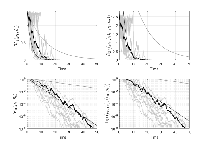
Figure 1: Exponential stabilization of the coupled 3-level quantum angular momentum system towards $(\boldsymbol{\rho}_{0},\boldsymbol{\rho}_{0})$ with the feedback controller (26) starting at $(\rho_{0},\hat{\rho}_{0})=(\boldsymbol{\rho}_{2},\boldsymbol{\rho}_{1})$ with $\omega=0.4$, $\eta=0.4$, $M=1.4$, $\hat{\omega}=0.5$, $\hat{\eta}=0.5$, $\hat{M}=1.5$, $\alpha=5$ and $\beta=2$: the black curves represent the mean value of 10 arbitrary sample trajectories, the light grey curves represent the exponential reference with exponent $\nu_{\textrm{av}}=-0.0761$, the dark grey curve represents the exponential reference with exponent $\nu_{\textrm{s}}=-0.3561$. The figures at the bottom are the semi-log versions of the ones at the top.

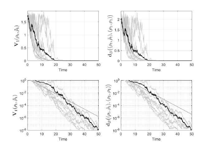
Figure 2: Exponential stabilization of the coupled 3-level quantum angular momentum system towards $(\boldsymbol{\rho}_{1},\boldsymbol{\rho}_{1})$ with the feedback controller (27) starting at $(\rho_{0},\hat{\rho}_{0})=(\mathrm{diag}(0.2,0.2,0.6),\mathrm{diag}(0.3,0.3,0.4))\in\mathrm{int}(\mathcal{S}_{N})\times\mathrm{int}(\mathcal{S}_{N})$ with $\omega=0.4$, $\eta=0.4$, $M=1.4$, $\hat{\omega}=0.5$, $\hat{\eta}=0.5$, $\hat{M}=1.5$, $\alpha=5$ and $\beta=2$: the black curves represent the mean value of 10 arbitrary sample trajectories, the light grey curves represent the exponential reference with exponent $\nu_{\textrm{s}}=-0.28$. The figures at the bottom are the semi-log versions of the ones at the top.

6 Conclusion and perspectives

In this paper, we proved a general exponential stabilization result for $N$-level quantum angular momentum systems, robust with respect to imprecise choices of the estimated physical parameters and wrong initialization of the estimated state. Such a robustness property was obtained by analyzing the asymptotic behavior of the coupled system describing the evolution of the quantum state and the associated estimated state. More precisely, we showed exponential stabilization of the coupled system towards a pair $(\boldsymbol{\rho}_{\bar{n}},\boldsymbol{\rho}_{\bar{n}})$, with $\boldsymbol{\rho}_{\bar{n}}$ being a chosen eigenstate of the measurement operator $J_{z}$. Furthermore, we gave explicit examples of stabilizing feedback control laws. Future research lines will concern the robustness properties of the stabilizing feedback controller in presence of delays for $N$-level quantum angular momentum systems and the adaptation of the robust exponential stabilization results to general open quantum systems.

References

• [1] H. Amini, C. Pellegrini, and P. Rouchon, Stability of continuous-time quantum filters with measurement imperfections, Russian Journal of Mathematical Physics, 21 (2014), pp. 297–315.
• [2] P. H. Baxendale, Invariant measures for nonlinear stochastic differential equations, in Lyapunov Exponents, Springer, 1991, pp. 123–140.
• [3] V. P. Belavkin, On the theory of controlling observable quantum systems, Avtomatika i Telemekhanika, (1983), pp. 50–63.
• [4] V. P. Belavkin, Nondemolition measurements, nonlinear filtering and dynamic programming of quantum stochastic processes, in Modeling and Control of Systems, Springer, 1989, pp. 245–265.
• [5] V. P. Belavkin, Quantum stochastic calculus and quantum nonlinear filtering, Journal of Multivariate analysis, 42 (1992), pp. 171–201.
• [6] V. P. Belavkin, Quantum filtering of markov signals with white quantum noise, in Quantum communications and measurement, Springer, 1995, pp. 381–391.
• [7] I. Bengtsson and K. Życzkowski, Geometry of quantum states: an introduction to quantum entanglement, Cambridge University Press, 2017.
• [8] T. Benoist and C. Pellegrini, Large time behavior and convergence rate for quantum filters under standard non demolition conditions, Communications in Mathematical Physics, 331 (2014), pp. 703–723.
• [9] L. Bouten and R. van Handel, On the separation principle in quantum control, in Quantum stochastics and information: statistics, filtering and control, World Scientific, 2008, pp. 206–238.
• [10] L. Bouten, R. van Handel, and M. R. James, An introduction to quantum filtering, SIAM Journal on Control and Optimization, 46 (2007), pp. 2199–2241.
• [11] G. Cardona, A. Sarlette, and P. Rouchon, Exponential stochastic stabilization of a two-level quantum system via strict lyapunov control, in IEEE Conference on Decision and Control, 2018, pp. 6591–6596.
• [12] G. Cardona, A. Sarlette, and P. Rouchon, Exponential stabilization of quantum systems under continuous non-demolition measurements, Automatica, 112 (2020), p. 108719.
• [13] H. Carmichael, An open systems approach to quantum optics, Springer-Verlag, Berlin Heidelberg New-York, 1993.
• [14] E. B. Davies, Quantum stochastic processes, Communications in Mathematical Physics, 15 (1969), pp. 277–304.
• [15] E. B. Davies, Quantum theory of open systems, Academic Press, 1976.
• [16] B. Hacker, S. Welte, S. Daiss, A. Shaukat, S. Ritter, L. Li, and G. Rempe, Deterministic creation of entangled atom–light schrödinger-cat states, Nature Photonics, 13 (2019), pp. 110–115.
• [17] R. L. Hudson and K. R. Parthasarathy, Quantum Ito’s formula and stochastic evolutions, Communications in Mathematical Physics, 93 (1984), pp. 301–323.
• [18] G. Kallianpur, Stochastic filtering theory, vol. 13, Springer Science & Business Media, 2013.
• [19] R. Khasminskii, Stochastic stability of differential equations, vol. 66, Springer, 2011.
• [20] W. Liang, N. H. Amini, and P. Mason, On exponential stabilization of spin-$\frac{1}{2}$ systems, in IEEE Conference on Decision and Control, 2018, pp. 6602–6607.
• [21] W. Liang, N. H. Amini, and P. Mason, On exponential stabilization of $N$-level quantum angular momentum systems, SIAM Journal on Control and Optimization, 57 (2019), pp. 3939–3960.
• [22] W. Liang, N. H. Amini, and P. Mason, On estimation and feedback control of spin-$\frac{1}{2}$ systems with unknown initial states, to appear in International Federation of Automatic Control World Congress, arXiv:1912.01074, (2020).
• [23] W. Liang, N. H. Amini, and P. Mason, On the robustness of stabilizing feedbacks of quantum spin-$\frac{1}{2}$ systems, submitted, arXiv:2004.05638, (2020).
• [24] X. Mao, Stochastic differential equations and applications, Woodhead Publishing, 2007.
• [25] M. Mirrahimi and R. van Handel, Stabilizing feedback controls for quantum systems, SIAM Journal on Control and Optimization, 46 (2007), pp. 445–467.
• [26] M. A. Nielsen and I. Chuang, Quantum computation and quantum information, Cambridge University Press, 2002.
• [27] L. G. Rogers and D. Williams, Diffusions, Markov processes and martingales: Volume 2, Itô calculus, vol. 2, Cambridge university press, 2000.
• [28] C. Sayrin, I. Dotsenko, X. Zhou, B. Peaudecerf, T. Rybarczyk, S. Gleyzes, P. Rouchon, M. Mirrahimi, H. Amini, M. Brune, J.-M. Raimond, and S. Haroche, Real-time quantum feedback prepares and stabilizes photon number states, Nature, 477 (2011), pp. 73–77.
• [29] D. W. Stroock and S. R. Varadhan, On the support of diffusion processes with applications to the strong maximum principle, in Proceedings of the Sixth Berkeley Symposium on Mathematical Statistics and Probability (Univ. California, Berkeley, Calif., 1970/1971), vol. 3, 1972, pp. 333–359.
• [30] K. Tsumura, Global stabilization at arbitrary eigenstates of N-dimensional quantum spin systems via continuous feedback, in American Control Conference, 2008, 2008, pp. 4148–4153.
• [31] R. van Handel, The stability of quantum markov filters, Infinite Dimensional Analysis, Quantum Probability and Related Topics, 12 (2009), pp. 153–172.
• [32] R. van Handel, J. K. Stockton, and H. Mabuchi, Feedback control of quantum state reduction, IEEE Transactions on Automatic Control, 50 (2005), pp. 768–780.