A Natural Actor-Critic Algorithm with
Downside Risk Constraints

Abstract

Existing work on risk-sensitive reinforcement learning — both for symmetric and downside risk measures — has typically used direct Monte-Carlo estimation of policy gradients. While this approach yields unbiased gradient estimates, it also suffers from high variance and decreased sample efficiency compared to temporal-difference methods. In this paper, we study prediction and control with aversion to downside risk which we gauge by the lower partial moment of the return. We introduce a new Bellman equation that upper bounds the lower partial moment, circumventing its non-linearity. We prove that this proxy for the lower partial moment is a contraction, and provide intuition into the stability of the algorithm by variance decomposition. This allows sample-efficient, on-line estimation of partial moments. For risk-sensitive control, we instantiate Reward Constrained Policy Optimization, a recent actor-critic method for finding constrained policies, with our proxy for the lower partial moment. We extend the method to use natural policy gradients and demonstrate the effectiveness of our approach on three benchmark problems for risk-sensitive reinforcement learning.

1 Introduction

Reinforcement learning (RL) solves the problem of how to act optimally in a potentially unknown environment. While it does this very well in many cases, it has become increasingly clear that uncertainty about the environment — both epistemic and aleatoric in nature — can have severe consequences on the performance of our algorithms. While many problems can be solved by maximising the expected returns alone, it is rarely sufficient, and shies away from many of the subtleties of the real-world. In fields such as finance and health, the mitigation of risk is absolutely foundational, and the lack of practical methods is one of the biggest roadblocks in wider adoption of RL. Now, recent developments in risk-sensitive RL have started to enable practitioners to design algorithms to tackle their problems. However, many of these approaches rely on full trajectory rollouts, and most only consider variance-related risk criteria which: 1. are not suited to all domains; and 2. are often non-trivial to estimate in an on-line setting. We rarely have the luxury of ready access to high-quality data, and our definition of risk is usually nuanced [1, 2].

This observation is not unique and indeed many fields have questioned the use of symmetric risk measures to correctly capture human preferences. Markowitz himself noted, for example, that “semi-variance seems a more plausible measure of risk than variance, since it is only concerned with adverse deviations” [3]. Yet, save for Tamar et al. [4] — who introduce semi-deviation as a possible measure of risk — very little work has been done to address this gap in RL research. Furthermore, of those that do, even fewer still consider the question of how to learn an incremental approximation, instead opting to directly estimate policy gradients with sampling.

The first contribution of this work lies in the development of the lower partial moment (LPM) — i.e. the expected value of observations falling below some threshold — as an effective downside risk measure that can be approximated efficiently through temporal-difference learning. This insight derives from the sub-additivity of the $\max$ function and enables us to define a recursive bound on the LPM that serves as a proxy in constrained policy optimisation. We are able to prove that the associated Bellman operator is a contraction, and analyse the variance on the transformed reward that emerges from the approximation to gain insight into the stability of the proposed algorithm. The second key contribution is to show that the Reward Constrained Policy Optimisation framework (RCPO) of Tessler et al. [5] can be extended to use natural policy gradients. While multi-objective problems in RL are notoriously hard to solve [6], natural gradients are known to address some of the issues associated with convergence to local minima. The resulting algorithm used alongside our LPM estimation procedure is easy to implement and is shown to be highly effective in a number of problem settings.

Related work.

Past work on risk-sensitivity and robustness in RL can be split into those that tackle epistemic uncertainty, and those that tackle aleatoric uncertainty – which is the focus of this paper. Aleatoric risk (the risk inherent to a problem) has received much attention in the literature. For example, in 2001, Moody and Saffell devised an incremental formulation of the Sharpe ratio for on-line learning. Shen et al. [8] later designed a host of value-based methods using utility functions (see also [9]), and work by Tamar et al. [10] and Sherstan et al. [11] even tackle the estimation of the variance on returns; a contribution closely related to those in this paper. More recently, a large body of work that uses policy gradient methods for risk-sensitive RL has emerged [12, 5, 13, 4]. Epistemic risk (the risk associated with, e.g., known model inconsistencies) has also been addressed, though to a lesser extent [14, 15, 16]. There also exists a distinct but closely related field called “safe RL” which includes approaches for safe exploration; see the excellent survey by Garcıa and Fernández [17].

2 Preliminaries

2.1 Markov decision processes

A regular discrete-time Markov decision process (MDP) comprises: a state space $\mathcal{S}$, (state-dependent) action space $\mathcal{A}(s)\subseteq\mathcal{A}$, and set of rewards $\mathcal{R}\subseteq\mathbb{R}$. The dynamics of the MDP are given by the state-transition probability distribution $p(s^{\prime}\mid s,a)$ with initial state distribution $d_{0}(s)$. The expected value of rewards generated for a state-action pair is denoted by $r(s,a)$. A policy $\pi_{\operatorname{\boldsymbol{\theta}}}(a\mid s)$, parameterised by the length $n$ vector $\operatorname{\boldsymbol{\theta}}\in\mathbb{R}^{n}$, assigns a probability density over the set of possible actions in a state $s$. We assume that $\pi$ is continuously differentiable with respect to $\operatorname{\boldsymbol{\theta}}$. For a given policy we define the return starting from time $t$ (in unified notation) by the sum of future rewards, $G_{t}\operatorname{\triangleq}\sum_{k=0}^{T}\gamma^{k}R_{t+k+1}$, where $\gamma\in[0,1]$ is the discount rate and $T$ is the terminal time [18]; we require that either $\gamma<1$ or $T<\infty$ to keep values finite. Value functions are then defined as expectations over the returns generated from a given state $v_{\pi}(s)\operatorname{\triangleq}\operatorname{\mathbb{E}}_{\pi}[G_{t}\mid S_{t}=s]$, or state-action pair $q_{\pi}(s,a)\operatorname{\triangleq}\operatorname{\mathbb{E}}_{\pi}[G_{t}\mid S_{t}=s,A_{t}=a]$. Here, the expectations with subscript $\pi$ are taken with respect to the implied trajectory distribution; where $\operatorname{\boldsymbol{\theta}}$ is usually omitted from $\pi_{\operatorname{\boldsymbol{\theta}}}$ for clarity. The goal of control in RL is to find a policy $\pi_{\operatorname{\boldsymbol{\theta}}^{\star}}$ that maximises the expected return from all start states, denoted by the reward-to-go objective $J_{R}(\operatorname{\boldsymbol{\theta}})\operatorname{\triangleq}\operatorname{\mathbb{E}}_{\pi}[G_{0}\mid d_{0}(\cdot)]$.

2.2 Actor-critic methods and natural policy gradients

Actor-critic (AC) methods are an important class of algorithms for optimising continuously differentiable policies. They leverage the policy gradient theorem [19] to update $\operatorname{\boldsymbol{\theta}}$ in the steepest ascent direction of $J_{R}(\operatorname{\boldsymbol{\theta}})$, which is typically expressed by the derivative

$$\frac{\partial J_{R}(\operatorname{\boldsymbol{\theta}})}{\partial\operatorname{\boldsymbol{\theta}}}=\int_{\mathcal{S}}d_{\pi_{\operatorname{\boldsymbol{\theta}}}}(s)\int_{\mathcal{A}(s)}\frac{\partial\pi_{\operatorname{\boldsymbol{\theta}}}(a\mid s)}{\partial\operatorname{\boldsymbol{\theta}}}q_{\pi_{\operatorname{\boldsymbol{\theta}}}}(s,a)\,\mathrm{d}a\,\mathrm{d}s,$$ (1)

where $d_{\pi}(s)$ denotes the discounted state distribution [20]. Using the log-likelihood trick [21] we can derive sample-based estimators for this expectation (as in REINFORCE [21]) but these are known to suffer from high variance. AC methods instead replace $q_{\pi}(s,a)$ with an estimate of the action-value function, $\hat{q}_{\pi}(s,a)$, parameterised by weights $\boldsymbol{w}_{q}\in\mathbb{R}^{n}$. This critic is learnt through policy evaluation and results in improved stability and sample efficiency. This can always be done without introducing bias via compatible function approximation (CFA), such that $\nabla_{\boldsymbol{w}_{q}}\hat{q}_{\pi}(s,a)=\nabla_{\operatorname{\boldsymbol{\theta}}}\log{\pi_{\operatorname{\boldsymbol{\theta}}}(a\mid s)}$ and the weights $\boldsymbol{w}_{q}$ minimise the mean-squared error (MSE) between $\hat{q}_{\pi}(s,a)$ and $q_{\pi}(s,a)$. “Vanilla” policy gradient methods like these, however, often get stuck in local optima [22]. Natural gradients, denoted by $\widetilde{\nabla}_{\operatorname{\boldsymbol{\theta}}}J(\operatorname{\boldsymbol{\theta}})$, avoid this by following the steepest ascent direction with respect to the Fisher metric rather than in standard Euclidean space. When combined with CFA, this gradient is given by the weights $\boldsymbol{w}_{q}$ of the critic, i.e. an update of the form $\operatorname{\boldsymbol{\theta}}\leftarrow\operatorname{\boldsymbol{\theta}}+\eta\,\boldsymbol{w}_{q}$; a rather beautiful result [23].

2.3 Constrained MDPs and RCPO

Constrained MDPs are a generalisation of MDPs to problems in which the optimal policy must also satisfy a set of behavioural requirements [24]. These constraints are represented by a penalty function $c(s,a)$ (akin to the reward function), constraint functions $C(s)=\operatorname{\mathbb{E}}_{\pi}[\sum_{k=0}^{T}\gamma^{k}c(s,a)\mid S_{t+k}=s]$ and $C(s,a)=\operatorname{\mathbb{E}}_{\pi}[\sum_{k=0}^{T}\gamma^{k}c(s,a)\mid S_{t+k}=s,A_{t+k}=a]$ over the realised penalties (with some abuse of notation), and threshold $\nu\in\mathbb{R}$. As in Tessler et al. [5], we denote the objective associated with the constraint function by $J_{C}(\operatorname{\boldsymbol{\theta}})=\operatorname{\mathbb{E}}_{\pi}[C_{\pi}(s)\mid d_{0}(\cdot)]$ such that the optimisation problem may be expressed by the mean-risk model

$$\max_{\pi\in\Pi} J_{R}(\operatorname{\boldsymbol{\theta}}),$$ (2)

subject to $$J_{C}(\operatorname{\boldsymbol{\theta}})\leq\nu,$$

where $\Pi$ is the space of policies. Constrained optimisation problems like this are then typically recast as saddle-point problems by Lagrange relaxation [25]:

$$\min_{\lambda\geq 0}\max_{\operatorname{\boldsymbol{\theta}}}\mathcal{L}(\lambda,\operatorname{\boldsymbol{\theta}})=\min_{\lambda\geq 0}\max_{\operatorname{\boldsymbol{\theta}}}\left[J_{R}(\operatorname{\boldsymbol{\theta}})-\lambda\cdot\left(J_{C}(\operatorname{\boldsymbol{\theta}})-\nu\right)\right],$$ (3)

where $\mathcal{L}$ denotes the Lagrangian, and $\lambda\geq 0$ the Lagrange multiplier. Feasible solutions are those that satisfy the constraint, the existence of which depends on the particular problem and choice of $c(s,a)$ and $\nu$. Any policy that is not a feasible solution is considered sub-optimal. Approaches to solving problems of this kind then revolve around the derivation and estimation of the gradients of $\mathcal{L}$ w.r.t. the policy parameters $\operatorname{\boldsymbol{\theta}}$ and multiplier $\lambda$ [26, 27]. Recent work by Tessler et al. [5] extended these techniques to handle general constraints without prior knowledge, while remaining invariant to reward scaling. Their algorithm, named RCPO, is a multi-timescale stochastic approximation algorithm with provable convergence guarantees under standard assumptions. RCPO’s updates take the form

$$\nabla_{\operatorname{\boldsymbol{\theta}}}\mathcal{L} =\operatorname{\mathbb{E}}_{\pi}\left[\nabla_{\operatorname{\boldsymbol{\theta}}}\log\pi_{\operatorname{\boldsymbol{\theta}}}(s,a)\left[q_{\pi}(s,a)-\lambda C_{\pi}(s,a)\right]\right],$$ (4)

$$\nabla_{\lambda}\mathcal{L} =\nu-C_{\pi}(s).$$ (5)

3 Downside Risk Measures

In general, the choice of $c(s,a)$ depends on the problem and desired behaviour, which need not always be motivated by risk. For example, in robotics problems, this may take the form of a cost applied to policies with a large jerk or snap in order to encourage smooth motion. In economics and health problems, the constraint is typically based on some measure of risk/dispersion associated with the uncertainty in the outcome, such as the variance. However, in many real world applications, it is more appropriate to consider downside risk, such as the dispersion of returns below a target threshold, or the likelihood of Black Swan events. Intuitively, we may think of a general risk measure as a measure of “distance” between risky situations and those that are risk-free, when both favourable and unfavourable discrepancies are accounted for equally. A downside risk measure, on the other hand, only accounts for deviations that contribute unfavourably to risk [28, 29].

3.1 Partial Moments

Partial moments were first introduced as a means of measuring the probability-weighted deviations below (or above) a target threshold $\tau$. These feature prominently in finance and statistical modelling as a means of defining (asymmetrically) risk-adjusted metrics of performance [30, 31, 32, 33]. Our definition of partial moments, stated below, follows the original formulation of Fishburn [34].

Definition 1.

Let $\tau\in\mathbb{R}$ denote a target value, then the $m$^th-order partial moments of the random variable $X$ about $\tau$ are given by

$$\operatorname{\mathbb{M}}_{\pm}^{m}[X\mid\tau]\operatorname{\triangleq}\mp\operatorname{\mathbb{E}}[(\tau-X)^{m}_{\pm}],$$ (6)

where $(x)_{+}\equiv\max{\{x,0\}}$, $(x)_{-}\equiv\min{\{x,0\}}$, and $m\in[1,\infty)$.

The two quantities $\operatorname{\mathbb{M}}^{m}_{-}[X\mid\tau]$ and $\operatorname{\mathbb{M}}^{m}_{+}[X\mid\tau]$ are known as the lower and upper partial moments (LPM/UPM), respectively. When the target is chosen to be the mean — i.e. $\tau=\operatorname{\mathbb{E}}[X]$ — we refer to them as the centralised partial moments, and typically drop $\tau$ from the notation for brevity. For example, the semi-variance is given by the centralised, second-order LPM: $\operatorname{\mathbb{M}}_{-}^{2}\left[X\right]$. Unlike the expectation operator, (6) are non-linear functions of the input and satisfy very few of the properties that make expected values well behaved. Of particular relevance to this work is the fact that they are non-additive. This presents a challenge in the context of approximation since we cannot directly apply the Robbins-Monro algorithm [35]. As we will show in Section 4, however, we can estimate an upper bound for the first partial moment, for which we introduce the following key property:

Lemma 1 (Subadditivity).

Consider a pair of random variables $X$ and $Y$, and a fixed, additive target $\tau=\tau_{X}+\tau_{Y}$. Then for $m=1$, the partial moment is subadditive in $X$ and $Y$:

$$\operatorname{\mathbb{M}}_{\pm}[X+Y\mid\tau]\leq\operatorname{\mathbb{M}}_{\pm}[X\mid\tau_{X}]+\operatorname{\mathbb{M}}_{\pm}[Y\mid\tau_{Y}].$$ (7)

Proof.

Consider the lower partial moment, expressing the inner term as a function of real and absolute values $\left[|\tau-X-Y|+\tau-X-Y\right]/2$. By the subadditivity of the absolute function (triangle inequality), it follows that:

$$\left(\tau-X-Y\right)_{+}=\left(\tau_{X}-X+\tau_{Y}-Y\right)_{+}\leq\left(\tau_{X}-X\right)_{+}+\left(\tau_{Y}-Y\right)_{+}.$$ (8)

By the linearity of the expectation operator, we arrive at (7). This result may also be derived for the upper partial moment by the same logic. ∎

Motivating example.

Figure 1: Simple MDP with two actions and 7 states; the terminal state is omitted.

(a) $\mathbb{V}[G]$

(b) $\operatorname{\mathbb{E}}[G]-\mathbb{V}[G]$

(c) $\operatorname{\mathbb{M}}_{-}[G\mid 0]$

(d) $\operatorname{\mathbb{E}}[G]-\operatorname{\mathbb{M}}_{-}[G\mid 0]$

Figure 2: Moments of the return $G$ generated by the MDP in Fig. 1. The x-axis corresponds to $\theta_{1}\in[0,1]$, and the y-axis to $\theta_{2}\in[0,1]$. Higher values are in yellow, and lower values in dark blue.

Why is this so important? Consider the MDP in Fig. 2, with stochastic policy parametrised by $\operatorname{\boldsymbol{\theta}}_{1,2}\in[0,1]$ such that $\pi(\rightarrow\mid s_{0})=\theta_{1}$ and $\pi(\uparrow\mid s_{\leftarrow})=\pi(\uparrow\mid s_{\rightarrow})=\theta_{2}$. As shown by Tamar et al. [12], even in a simple problem such as this, the space of solutions for a mean-variance criterion is non-convex. Indeed, Fig. 2 shows that the solution space exhibits local-optima for the deterministic policies $\operatorname{\boldsymbol{\theta}}_{1,2}\in\{(0,0),(1,0),(0,1)\}$. On the other hand, the lower partial moment only exhibits a single optimum at the correct solution of $\operatorname{\boldsymbol{\theta}}_{1}=\operatorname{\boldsymbol{\theta}}_{2}=1$. While this is certainly not proof that such phenomena occur in all cases, it does suggest that partial moments have a valid place in risk-averse RL, and may in some instances lead to more amenable learning.

4 Prediction

Our objective in this section is now to derive an incremental, temporal-difference prediction algorithm for the first LPM of the return distribution $G_{t}$. To begin, let $\rho[\tau](s,a)$ denote the first LPM of $G_{t}$ with respect to a target function $\tau(s,a)$, starting from state-action pair $(s,a)$, by

$$\rho[\tau](s,a)\operatorname{\triangleq}\operatorname{\mathbb{M}}_{-}[G_{t}\mid S_{t}=s,A_{t}=a,\tau(s,a)],$$ (9)

where the centralised moments are shortened to $\rho(s,a)$. For a given target, this function can be learnt trivially through Monte-Carlo (MC) estimation using batches of sample trajectories. Indeed, we can even learn the higher-order moments using such an approach. However, while this yields an unbiased estimate of the LPM, it comes at the cost of increased variance and decreased sample efficiency [18]. This is especially pertinent in risk-sensitive RL which is often concerned with (already) highly stochastic domains. The challenge is that (9) is a non-linear function of $G_{t}$ which does not have a direct recursive form amenable to TD-learning.

Rather than learn the LPM directly, we instead learn a proxy in the form of an upper bound. To begin, we note that by Lemma 1, the LPM of the return distribution satisfies

$$\rho[\tau](s,a)\leq\operatorname{\mathbb{M}}_{-}\left[R_{t+1}\mid\tau_{R}(s,a)\right]+\gamma\operatorname{\mathbb{M}}_{-}\left[G_{t+1}\mid\tau(s^{\prime},a^{\prime})\right],$$ (10)

for $\tau(s,a)=\tau_{R}(s,a)+\gamma\operatorname{\mathbb{E}}_{\pi}[\tau(s^{\prime},a^{\prime})]$. Unravelling the final term ad infinitum yields a geometric series of bounds on the reward moments. This sum admits a recursive form

$$\varrho[\tau](s,a)\operatorname{\triangleq}\operatorname{\mathbb{M}}_{-}[R_{t+1}\mid\tau_{R}]+\gamma\varrho[\tau](s^{\prime},a^{\prime}),$$ (11)

which is, precisely, an action-value function with non-linear reward transformation: $g(r)={(\tau_{R}-r)}_{+}$. This means we are free to use any prediction algorithm to perform the actual TD updates, such as SARSA or GQ($\lambda$) [36]. We now only need to choose $\tau_{R}$ to satisfy our requirements; perhaps to minimise the error between (9) and (11). For example, a fixed target yields the expression $\tau_{R}(s,a)=(1-\gamma)\tau$. Alternatively, a centralised variant would be given by $\tau_{R}(s,a)=r(s,a)$. This freedom to choose a target function affords us a great deal of flexibility in designing downside risk metrics.

Convergence.

As noted by van Hasselt et al. [37], Bellman equations with non-linear reward transformations (i.e. (11)) carry over all standard convergence results under the assumption that the transformation is bounded. This is trivially satisfied when the rewards themselves are bounded [38]. This means that the associated Bellman operator is a contraction, and that the proxy converges with stochastic approximation under the standard Robbins-Monro conditions [35].

Lemma 2.

The variance on a random variable $X\in\mathbb{R}$ satisfies the inequality $\mathbb{V}[(c-X)_{+}]\leq\mathbb{V}[X]$ for arbitrary constant $c\in\mathbb{R}$.

Variance analysis.

Lemma 2 (proof of which is in the appendix) can be used to show that the non-linear reward term in (11) exhibits a lower variance than that of the original reward: $\mathbb{V}[g(R)]\leq\mathbb{V}[R]$. While we provide no formal proof, this observation suggests that the variances on the corresponding Bellman equations satisfy an inequality in the same direction. This motivates the use of our proposed LPM proxy compared to prediction methods of higher order moments, which, by definition, will suffer from increased variance, and may therefore be less stable.

5 Control

In the previous section we saw how the upper bound on the LPM of the return can be learnt effectively in an incremental fashion. Putting this to use now requires that we integrate our estimator into a constrained policy optimisation framework. This is particularly simple in the case of RCPO, for which we incorporate (11) into the penalised reward function introduced in Def. 3 [5]. Following their template, we may derive a whole class of actor-critic algorithms that optimise for a downside risk-adjusted objective, including those that make use of natural gradients.

Theorem 1 (Compatible function approximation).

If both $\hat{q}(s,a)$ and $\hat{\varrho}[\tau](s,a)$ are compatible

$$\psi(s,a)\operatorname{\triangleq}\frac{\partial\hat{q}(s,a)}{\partial\boldsymbol{w}_{q}}=\frac{\partial\hat{\varrho}[\tau](s,a)}{\partial\boldsymbol{w}_{\varrho}}=\frac{1}{\pi_{\operatorname{\boldsymbol{\theta}}}(a\mid s)}\frac{\partial\pi_{\operatorname{\boldsymbol{\theta}}}(a\mid s)}{\partial\operatorname{\boldsymbol{\theta}}},$$ (12)

and independently minimise the errors

$$\mathcal{E}_{q}^{2}\operatorname{\triangleq}\operatorname{\mathbb{E}}\left[{\left(\psi{(s,a)}^{\top}\cdot\boldsymbol{w}_{q}-q(s,a)\right)}^{2}\right],\quad\mathcal{E}_{\varrho}^{2}\operatorname{\triangleq}\operatorname{\mathbb{E}}\left[{\left(\psi{(s,a)}^{\top}\cdot\boldsymbol{w}_{\varrho}-\varrho[\tau](s,a)\right)}^{2}\right],$$ (13)

then we can replace $q(s,a)-\lambda\varrho[\tau](s,a)$ with $\hat{q}(s,a)-\lambda\hat{\varrho}[\tau](s,a)$ to get

$$\widetilde{\nabla}_{\operatorname{\boldsymbol{\theta}}}\mathcal{L}(\lambda,\operatorname{\boldsymbol{\theta}})=\frac{\partial\mathcal{L}(\lambda,\operatorname{\boldsymbol{\theta}})}{\partial\operatorname{\boldsymbol{\theta}}}=\int_{\mathcal{S}}d_{\pi_{\operatorname{\boldsymbol{\theta}}}}(s)\int_{\mathcal{A}(s)}\frac{\partial\pi_{\operatorname{\boldsymbol{\theta}}}(a\mid a)}{\partial\operatorname{\boldsymbol{\theta}}}\left[\hat{q}(s,a)-\lambda\hat{\varrho}[\tau](s,a)\right]\,\mathrm{d}a\,\mathrm{d}s.$$ (14)

Crucially, if the two value function estimators $\hat{q}(s,a)$ and $\hat{\varrho}[\tau](s,a)$ are compatible with the policy parameterisation [19], then we may extend RCPO to use natural policy gradients (see Section 2.2). We call the resulting algorithm NRCPO for which the existence hinges on Theorem 1 above; a proof is provided in the appendix. This shows under which conditions the true value functions may be replaced with the function approximators, without introducing bias. Assuming the conditions are met, it remains only to replace the “vanilla” gradient in Eq. 4 with the natural gradient. This yields a policy update

$$\operatorname{\boldsymbol{\theta}}\leftarrow\operatorname{\boldsymbol{\theta}}+\eta\left(\boldsymbol{w}_{q}-\lambda\boldsymbol{w}_{\varrho}\right),$$

which is not only trivial to implement, but also benefits from all the advantages associated with using natural gradients [22].

6 Numerical Experiments

Here we present evaluations of our proposed NRCPO algorithm on three experimental domains using variations on $\tau(s,a)$ in the LPM proxy (Eq. 11). The chosen hyperparameters and experimental configurations, unless otherwise stated, can be found in the appendix.

6.1 Multi-armed bandit

The first problem setting — taken from Tamar et al. [4] — is a 3-armed bandit with rewards distributed according to: $R_{A}\sim\mathcal{N}(1,1)$; $R_{B}\sim\mathcal{N}(4,6)$; and $R_{C}\sim\textrm{Pareto}(1,1.5)$. The expected reward from each arm is 1, 4 and 3, respectively. The optimal solution for a risk-neutral agent is to choose the second arm, but it is apparent that agents sensitive to negative values should choose the third arm since the Pareto distribution’s support is bounded from below.

Results.

We evaluated our proposed methods by training three different Boltzmann policies on the multi-armed bandit problem. The first (Fig. 3(a)) was trained using a standard variant of NAC, the latter two (Figs. 3(b) and 3(c)) used a stateless version of NRCPO with first and second LPMs as risk measures, respectively; for simplicity, we assume a constant value for the Lagrange multiplier $\lambda$. The results show that after $\sim 5000$ samples, both risk-averse policies have converged on arm $C$. This highlights the flexibility of our approach, and the improvements in efficiency that can be gained from incremental algorithms compared to Monte-Carlo estimation. See, for example, the approach of Tamar et al. [4] which used 10000 samples per gradient estimate, requiring $\sim 10^{5}$ sample trajectories before convergence.

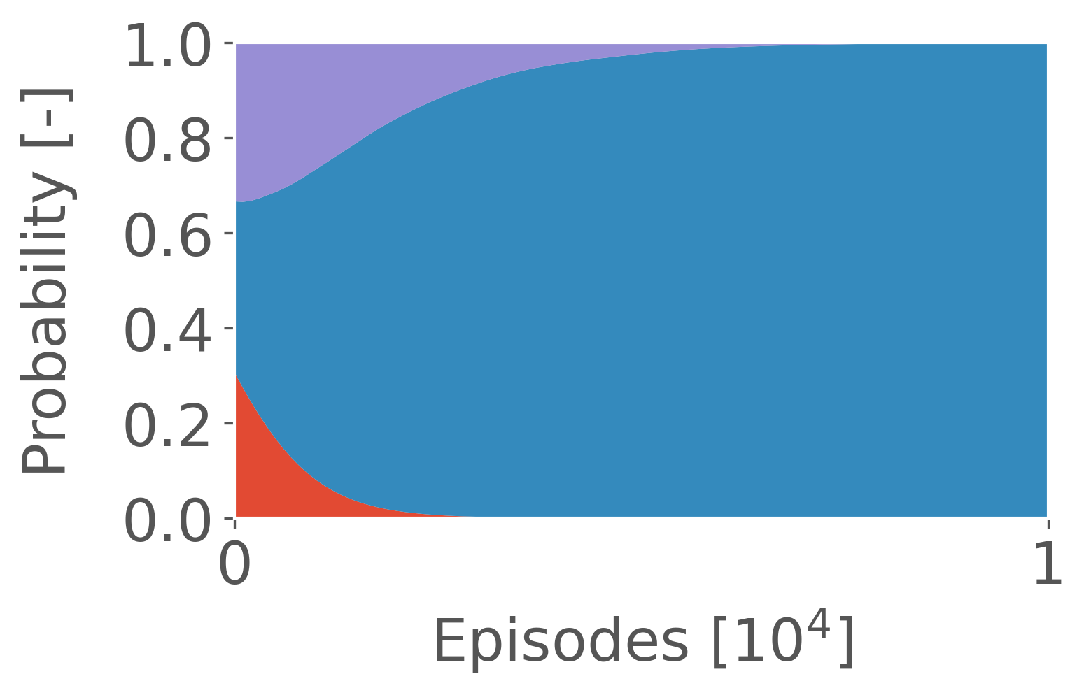
(a) $\operatorname{\mathbb{E}}[R]$

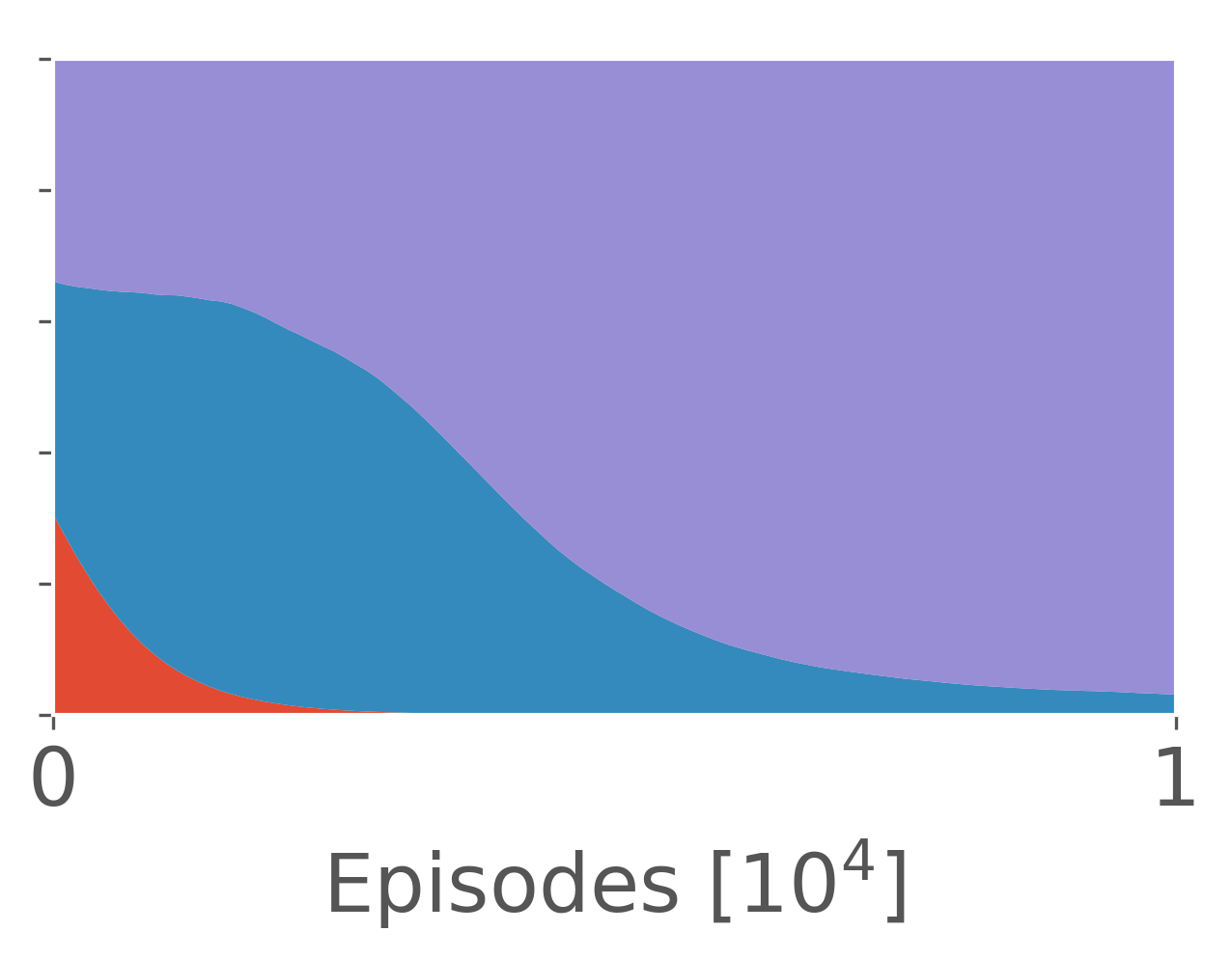
(b) $\operatorname{\mathbb{E}}[R]-2\operatorname{\mathbb{M}}_{-}[R]$

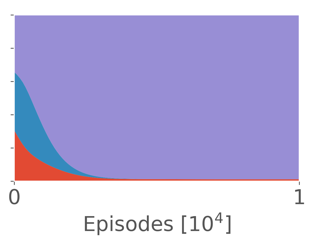
(c) $\operatorname{\mathbb{E}}[R]-\operatorname{\mathbb{M}}_{-}^{2}[R]$

Figure 3: Evolution of Boltzmann policies’ selection probabilities for arms A (red), B (blue) and C (purple). Each curve represents a normalised average over 100 independent trials.

6.2 Portfolio optimisation

The next setting is an adaptation of the portfolio optimisation problem first proposed by Tamar et al. [12], and featured in [13], as a motivating example of risk-averse RL in finance. Consider two types of asset: a liquid asset such as cash holdings with interest rate $r_{\text{L}}$; and an illiquid asset with time-dependent interest rate $r_{\text{N}}(t)\in\{\overline{r}_{\text{N}},\underline{r}_{\text{N}}\}$ that switches between two values stochastically. Unlike the original formulation, we do not assume that this happens symmetrically. Instead, we treat $r_{\text{N}}(t)$ as a switching process with two states and transition probabilities $p_{\uparrow}$ and $p_{\downarrow}$. At each timestep the agent chooses an amount (up to $M$) of the illiquid asset to purchase at a fixed cost per unit $\alpha$. At maturity (after $N$ steps) this illiquid asset either defaults (with probability $p_{\text{D}}$), or is sold and converted into liquid asset. The state space of the problem is embedded in $\mathbb{R}^{N+2}$, where the first entry denotes the allocation in the liquid asset, the next $N$ are the allocations in the non-liquid assets, and the final value is given by $r_{\text{N}}(t)-\operatorname{\mathbb{E}}_{t^{\prime}<t}[r_{\text{N}}(t^{\prime})]$. The actions are discrete choices for the purchase order, and the reward at each timestep is given by the log-return in the liquid asset between $t$ and $t+1$, as in [13].

Results.

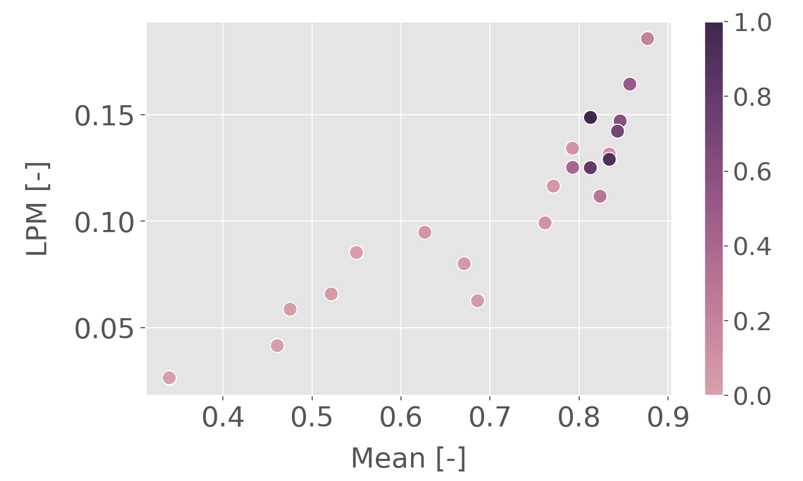
(a) Mean vs. the LPM of returns.

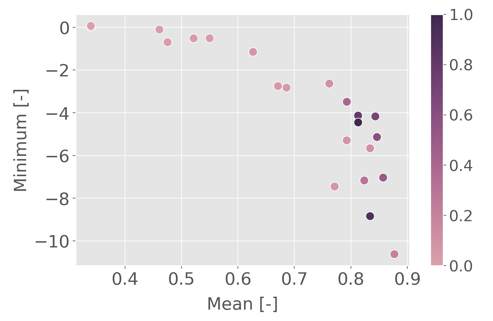
(b) Mean vs. the minimum observed return.

Figure 4: Performance of portfolio optimisation solutions for varying thresholds $\nu\in[0,1]$. Each point was generated by evaluating the policy over 10⁴ trials following training.

Figure 4 shows how the performance of our LPM variant of NRCPO performs on the portfolio optimisation problem; in this case we chose to use the centralised LPM as a target, i.e. set $\tau_{R}(s,a)=r(s,a)$. We observe the emergence of a “frontier” of solutions which trades-off maximisation of the expected return with minimisation of the risk penalty. As the threshold $\nu$ (see Eq. 2) increases (i.e. increasing tolerance to risk), so too do we see a tendency for solutions with a higher mean, higher LPM and more extreme minima. From this we can conclude that minimisation of the proxy (11) does have the desired effect of reducing the LPM, validating the practical value of the bound.

6.3 Optimal consumption

The final setting, known as Merton’s optimal consumption problem [39] is another example of intertemporal portfolio optimisation. This particular setting has been largely unstudied in the RL literature in spite of the fact that it represents a broad class of real-world problems; e.g. retirement planning. At each timestep the agent must specify two quantities: 1. the proportion of it’s wealth to invest in a risky asset (whose returns we assume to be Normally distributed) and a risk-free/liquid asset with deterministic return $r_{\text{L}}$, and 2. an amount of it’s wealth to consume and permanently remove from the portfolio. The problem terminates when all the agent’s wealth, $W_{t}$, is consumed or the terminal timestep is reached (200 steps). In the latter case, any remaining wealth that wasn’t consumed is lost. The state space is given by the current time and the agent’s remaining wealth, and the reward is defined to be the amount consumed. To highlight downside risk, we also extend the traditional model to include defaults. At each decision point there is a non-zero probability $p_{\text{D}}$ that the risky asset’s underlying “disappears”, the risky investment is lost, the problem terminates, and the remaining wealth in the liquid asset is consumed in it’s entirety.

Results.

In this case we defined a custom target function by leveraging prior knowledge of the problem. Specifically, we set $\tau_{R}(s,a)=W_{t}\cdot\Delta t(T-t)$, where $t$ and $T$ denote the current and terminal times, and $\Delta t$ is the time increment. This has the interpretation of the expected reward generated by an agent that consumes it’s wealth at a fixed rate. Unrolling the recursive definition of $\tau(s,a)$, we have an implied target of $W_{t}$ for all states. In other words, we associate a higher penalty with those policies that underperform said reasonable “benchmark” and finish the episode having consumed less wealth than the initial investment.

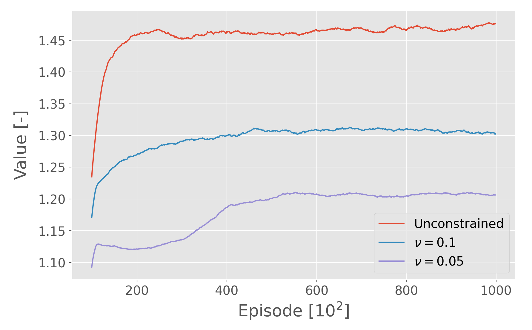
(a) $J_{R}(\operatorname{\boldsymbol{\theta}})$

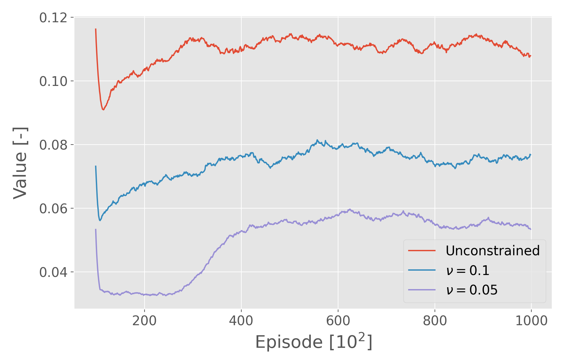
(b) $J_{C}(\operatorname{\boldsymbol{\theta}})$

Figure 5: Evolution of performance of optimal consumption solutions for $\nu\in\{0.05,0.1,\infty\}$. Each curve was generated by evaluating the policy for 100 trials every 100 training episodes, with a simple moving average of period 100 applied for clarity.

Figure 5 shows how performance of our algorithm evolved during training. Each curve was generated by sampling 100 trajectories every 100 training episodes to estimate statistics. As in the previous section, we observe how decreasing $\nu$ leads to increasing risk-aversion in the form of a lower mean and LPM. In all cases the algorithm was able to identify a feasible solution and exhibited highly stable learning. An important conclusion to take from this is that the flexibility to choose $\tau_{R}(s,a)$ affords us a great deal of control over the behaviour of the policy. In this case, we only penalise downside risk associated with losses. Furthermore, (N)RCPO removes the need for calibrating the multiplier $\lambda$, which can be very hard to tune [42]. This makes our approach highly practical for many real-world problems.

7 Conclusions

In this paper we have put forward two key ideas. First, that partial moments offer a tractable alternative to conventional metrics such as variance or conditional value at risk. We show that our proxy has a simple interpretation and enjoys favourable reward variance. Second, we demonstrate how an existing method in constrained policy optimisation can be extended to leverage natural gradients, an algorithm we call NRCPO. The combination of these two developments is a methodology for deriving downside risk-averse policies with a great deal of flexibility and sample efficiency. In future work we hope to address questions on computational complexity, and how these methods may be applied to multi-agent systems.

Software and Data.

All our code will be made freely accessible via GitHub.

Appendix A Variance Analysis

Lemma 2.

For any constant $c\in\mathbb{R}$, the variance, $\mathbb{V}[X]$, of a random variable $X$ that is supported on $\mathbb{R}$ satisfies $\mathbb{V}[(c-X)_{+}]\leq\mathbb{V}[X].$

Proof.

Let $Y\operatorname{\triangleq}c-X$ and $Z\operatorname{\triangleq}(Y)_{+}=(c-X)_{+}$. Since $c$ is a constant, $\mathbb{V}[Y]=\mathbb{V}[X]$. Thus, it suffices to show that $\mathbb{V}[Z]\leq\mathbb{V}[Y]$.

Denote by $p_{+}\operatorname{\triangleq}\mathbb{P}(Y\geq 0)$ and $p_{-}\operatorname{\triangleq}\mathbb{P}(Y<0)$, the probabilities of $Y$ being non-negative or negative respectively. Let $\mu_{+}\operatorname{\triangleq}\operatorname{\mathbb{E}}[Y\mid Y\geq 0]$ and $\mu_{-}\operatorname{\triangleq}\operatorname{\mathbb{E}}[Y\mid Y<0]$. Then we have:

$$\mu_{Y}\operatorname{\triangleq}\operatorname{\mathbb{E}}[Y] =p_{+}\mu_{+}+p_{-}\mu_{-},$$ (15)

$$\mu_{Z}\operatorname{\triangleq}\operatorname{\mathbb{E}}[Z] =p_{+}\mu_{+}.$$ (16)

Similarly, with $m_{+}^{2}\operatorname{\triangleq}\operatorname{\mathbb{E}}[Y^{2}\mid Y\geq 0]$ and $m_{-}^{2}\operatorname{\triangleq}\operatorname{\mathbb{E}}[Y^{2}\mid Y<0]$, the second moments are:

$$m_{Y}^{2}\operatorname{\triangleq}\operatorname{\mathbb{E}}[Y^{2}] =p_{+}m^{2}_{+}+p_{-}m^{2}_{-},$$ (17)

$$m_{Z}^{2}\operatorname{\triangleq}\operatorname{\mathbb{E}}[Z^{2}] =p_{+}m^{2}_{+},$$ (18)

Then we can express the variance of $Y$ and $Z$ as

$$\mathbb{V}[Y] =p_{+}m^{2}_{+}-p_{+}^{2}\mu^{2}_{+}+p_{-}m^{2}_{-}-2p_{+}p_{-}\mu_{+}\mu_{-}-p_{-}^{2}\mu^{2}_{-},$$ (19)

$$\mathbb{V}[Z] =p_{+}m^{2}_{+}-p_{+}^{2}\mu^{2}_{+}.$$ (20)

Their difference is

$$\mathbb{V}[Y]-\mathbb{V}[Z]=p_{-}m^{2}_{-}-2p_{+}p_{-}\mu_{+}\mu_{-}-p_{-}^{2}\mu^{2}_{-}.$$ (21)

We split this difference into two non-negative terms as follows.

$$p_{-}m^{2}_{-}-p_{-}^{2}\mu^{2}_{-} \geq 0,$$ (22)

$$-2p_{+}p_{-}\mu_{+}\mu_{-} \geq 0.$$ (23)

The first inequality follows from the fact that $\mathbb{V}[Y\mid Y<0]=m^{2}_{-}-\mu^{2}_{-}\geq 0$, so $m^{2}_{-}\geq\mu^{2}_{-}$ and $p_{-}\in[0,1]$. The second inequality follows from the facts that $p_{+},p_{-},\mu_{+}\geq 0$ and $\mu_{-}<0$. Thus, we have shown that $\mathbb{V}[Y]-\mathbb{V}[Z]\geq 0$, which completes the proof. ∎

Appendix B Compatible Function Approximation

We now show that, under certain conditions, we can use $\hat{q}(s,a)-\lambda\hat{\varrho}[\tau](s,a)$, instead of $q(s,a)-\lambda\varrho[\tau](s,a)$, to get an unbiased estimate of the policy gradient.

Theorem 1 (Compatible function approximation).

If the following three conditions hold:

1. $\hat{q}(s,a)$ and $\hat{\varrho}[\tau](s,a)$ are compatible with the policy $\pi_{\operatorname{\boldsymbol{\theta}}}$, i.e.,

   $$\frac{\partial\hat{q}(s,a)}{\partial\boldsymbol{w}_{q}}=\frac{\partial\hat{\varrho}[\tau](s,a)}{\partial\boldsymbol{w}_{\varrho}}=\frac{1}{\pi_{\operatorname{\boldsymbol{\theta}}}(a\mid s)}\frac{\partial\pi_{\operatorname{\boldsymbol{\theta}}}(a\mid s)}{\partial\operatorname{\boldsymbol{\theta}}};$$ (24)

2. $\hat{q}(s,a)$ minimises the error

   $$\mathcal{E}_{q}^{2}\operatorname{\triangleq}\operatorname{\mathbb{E}}\left[{\left(\hat{q}_{\boldsymbol{w}_{q}}(s,a)-q(s,a)\right)}^{2}\right],$$ (25)

3. and $\hat{\varrho}[\tau](s,a)$ minimises the error

   $$\mathcal{E}_{\varrho}^{2}\operatorname{\triangleq}\operatorname{\mathbb{E}}\left[{\left(\hat{\varrho}_{\boldsymbol{w}_{\varrho}}[\tau](s,a)-\varrho[\tau](s,a)\right)}^{2}\right],$$ (26)

then

$$\frac{\partial\mathcal{L}(\lambda,\operatorname{\boldsymbol{\theta}})}{\partial\operatorname{\boldsymbol{\theta}}}=\int_{\mathcal{S}}d_{\pi_{\operatorname{\boldsymbol{\theta}}}}(s)\int_{\mathcal{A}(s)}\frac{\partial\pi_{\operatorname{\boldsymbol{\theta}}}(a\mid a)}{\partial\operatorname{\boldsymbol{\theta}}}\left[\hat{q}(s,a)-\lambda\hat{\varrho}[\tau](s,a)\right]\,\mathrm{d}a\,\mathrm{d}s$$ (27)

is an unbiased estimate of the policy gradient.

Proof.

Let $f(s,a)$ be an arbitrary function of state and action and let there exist a corresponding approximator $\hat{f}(s,a)$ with weights $\boldsymbol{w}_{f}$. The MSE between the true function and approximation is given by

$$\mathcal{E}_{f}^{2}=\int_{\mathcal{S}}d_{\pi_{\operatorname{\boldsymbol{\theta}}}}(s)\int_{\mathcal{A}(s)}\pi_{\operatorname{\boldsymbol{\theta}}}(a\mid s)\left[\hat{f}(s,a)-f(s,a)\right]^{2}\text{d}a\text{d}s.$$ (28)

If $\hat{f}(s,a)$ fulfils requirement (24), then the derivative of the MSE is given by

$$\frac{\partial\mathcal{E}_{f}^{2}}{\partial\boldsymbol{w}_{f}} =2\int_{\mathcal{S}}d_{\pi_{\operatorname{\boldsymbol{\theta}}}}(s)\int_{\mathcal{A}(s)}\pi_{\operatorname{\boldsymbol{\theta}}}(a\mid s)\frac{\partial\hat{f}(s,a)}{\partial\boldsymbol{w}_{f}}\left[\hat{f}(s,a)-f(s,a)\right]\text{d}a\text{d}s,$$ (29)

$$=2\int_{\mathcal{S}}d_{\pi_{\operatorname{\boldsymbol{\theta}}}}(s)\int_{\mathcal{A}(s)}\frac{\partial\pi_{\operatorname{\boldsymbol{\theta}}}(a\mid s)}{\partial\operatorname{\boldsymbol{\theta}}}\left[\hat{f}(s,a)-f(s,a)\right]\text{d}a\text{d}s.$$ (30)

If we then assume that the learning method minimises the MSE defined above (i.e. requirements (25) and (26)), then the weights $\boldsymbol{w}_{f}$ give the stationary point. Equating the expression to zero thus results in the equality

$$\int_{\mathcal{S}}d_{\pi_{\operatorname{\boldsymbol{\theta}}}}(s)\int_{\mathcal{A}(s)}\frac{\partial\pi_{\operatorname{\boldsymbol{\theta}}}(a\mid a)}{\partial\operatorname{\boldsymbol{\theta}}}f(s,a)\text{d}a\text{d}s=\int_{\mathcal{S}}d_{\pi_{\operatorname{\boldsymbol{\theta}}}}(s)\int_{\mathcal{A}(s)}\frac{\partial\pi_{\operatorname{\boldsymbol{\theta}}}(a\mid a)}{\partial\operatorname{\boldsymbol{\theta}}}\hat{f}(s,a)\text{d}a\text{d}s,$$ (31)

where $f(s,a)$ may be replaced with either $q(s,a)$ or $\varrho[\tau](s,a)$ as needed. This means that we can interchange the true value functions in the policy gradient with the MSE-minimising approximations. This is the classic result of compatible function approximation originally presented by Sutton et al. [19].

Now, for an objective of the form $\mathcal{L}(\lambda,\operatorname{\boldsymbol{\theta}})=J_{R}(\operatorname{\boldsymbol{\theta}})-\lambda J_{C}(\operatorname{\boldsymbol{\theta}})$ (i.e. that used in RCPO), we have that

$$\frac{\partial\mathcal{L}(\lambda,\operatorname{\boldsymbol{\theta}})}{\partial\operatorname{\boldsymbol{\theta}}}=\frac{\partial J_{R}(\operatorname{\boldsymbol{\theta}})}{\partial\operatorname{\boldsymbol{\theta}}}-\lambda\frac{\partial J_{C}(\operatorname{\boldsymbol{\theta}})}{\partial\operatorname{\boldsymbol{\theta}}}.$$ (32)

From the policy gradient theorem [19], and the compatible function approximation result above, we also know that each of the differential terms may be expressed by an integral of the form

$$\frac{\partial J_{f}(\operatorname{\boldsymbol{\theta}})}{\partial\operatorname{\boldsymbol{\theta}}}=\int_{\mathcal{S}}d_{\pi_{\operatorname{\boldsymbol{\theta}}}}(s)\int_{\mathcal{A}(s)}\frac{\partial\pi_{\operatorname{\boldsymbol{\theta}}}(a\mid a)}{\partial\operatorname{\boldsymbol{\theta}}}\hat{f}(s,a)\,\mathrm{d}a\,\mathrm{d}s.$$ (33)

Combining (32) and (33), it follows from the linearity of integration (sum rule) that the policy gradient of the Lagrangian is given by (27). ∎

Appendix C Experiments

A template of our proposed algorithm NRCPO using the LPM as a constraint is outlined in Algorithm 1. This implementation includes a tweak to the traditional policy update that was first introduced by thomas2014bias in which the advantage weights are rescaled using $L_{2}$ normalisation. This was found to improve stability during learning.

Algorithm 1 NRCPO-LPM

1:  for $k\leftarrow 0,1\ldots$ do

2:     Initialise state $s_{0}\sim d_{0}(\cdot)$

3:     for $t\leftarrow 0,1\ldots,T-1$ do

4:        Sample action $a_{t}\sim\pi(\cdot\mid s_{t})$

5:        Observe new state $s_{t+1}$ and reward $R_{t+1}$

6:        Update critics: $\hat{q}(s_{t},a_{t})$ and $\hat{\varrho}[\tau](s_{t},a_{t})$

7:        if $t+1\bmod N_{\text{Policy}}=0$ then

8:           Update policy: $\boldsymbol{\theta}\leftarrow\eta\frac{\boldsymbol{w}_{q}-\lambda\boldsymbol{w}_{\varrho}}{||\boldsymbol{w}_{q}-\lambda\boldsymbol{w}_{\varrho}||_{2}}$

9:        end if

10:     end for

11:  end for

In the following subsections, we specify for each of the three experimental domains: the policy $\pi_{\operatorname{\boldsymbol{\theta}}}$; $\hat{q}(s,a)$ and $\hat{\varrho}[\tau](s,a)$; and the prediction algorithm used to estimate the weights $\boldsymbol{w}_{q}$ and $\boldsymbol{w}_{\varrho}$ in the “Update critics” step. We also state the values of any domain-specific parameters used during experiments.

C.1 Bandit

In the bandit problem we considered a Gibbs policy of the form

$$\pi_{\operatorname{\boldsymbol{\theta}}}(a)=\frac{e^{\theta_{a}}}{\sum_{b}e^{\theta_{b}}},$$ (34)

where each action corresponded to a unique choice over the three arms $a\in\{A,B,C\}$. The value functions were then represented by linear function approximators

$$\hat{q}(a) =\nabla_{\operatorname{\boldsymbol{\theta}}}\log\pi_{\operatorname{\boldsymbol{\theta}}}(a)^{\top}\boldsymbol{w}_{q}+v_{q},$$ (35)

$$\hat{\varrho}(a) =\nabla_{\operatorname{\boldsymbol{\theta}}}\log\pi_{\operatorname{\boldsymbol{\theta}}}(a)^{\top}\boldsymbol{w}_{\varrho}+v_{\varrho},$$ (36)

which are compatible with the policy by construction. The canonical SARSA algorithm was used for policy evaluation with learning rate of 0.005. The policy updates were performed every $N_{\text{Policy}}=100$ episodes with $\eta=0.001$.

C.2 Portfolio Optimisation

In the portfolio optimisation problem we again considered a Gibbs policy, but this time of the form

$$\pi_{\operatorname{\boldsymbol{\theta}}}(a\mid\boldsymbol{s})=\frac{e^{\boldsymbol{\phi}(\boldsymbol{s},a)^{\top}\operatorname{\boldsymbol{\theta}}}}{\sum_{b}e^{\boldsymbol{\phi}(\boldsymbol{s},b)^{\top}\operatorname{\boldsymbol{\theta}}}}.$$ (37)

Here, we chose to use a linear basis over the state space, with independent sets of activations for each action. That is,

$$\boldsymbol{\phi}(\boldsymbol{s},a)=\left[\boldsymbol{\phi}(\boldsymbol{s})^{\top}\circ\boldsymbol{1}^{\top}_{a\,=\,1},\ldots,\boldsymbol{\phi}(\boldsymbol{s})^{\top}\circ\boldsymbol{1}^{\top}_{a\,=\,|\mathcal{A}|}\right]^{\top}$$ (38)

where $\circ$ denotes the Hadamard product and the state-dependent basis is given by

$$\boldsymbol{\phi}(\boldsymbol{s})=\left[1,s_{1},s_{2},\ldots,s_{N}\right].$$ (39)

The value functions were then represented by linear function approximators

$$\hat{q}(a) =\nabla_{\operatorname{\boldsymbol{\theta}}}\log\pi_{\operatorname{\boldsymbol{\theta}}}(a\mid\boldsymbol{s})^{\top}\boldsymbol{w}_{q}+\boldsymbol{\phi}(\boldsymbol{s})^{\top}\boldsymbol{v}_{q},$$ (40)

$$\hat{\varrho}(a) =\nabla_{\operatorname{\boldsymbol{\theta}}}\log\pi_{\operatorname{\boldsymbol{\theta}}}(a\mid\boldsymbol{s})^{\top}\boldsymbol{w}_{\varrho}+\boldsymbol{\phi}(\boldsymbol{s})^{\top}\boldsymbol{v}_{\varrho},$$ (41)

which are compatible with the policy by construction. The canonical SARSA($\lambda$) algorithm was used for policy evaluation with learning rate of 0.0001, a discount factor of $\gamma=0.99$ and accumulating trace with rate $\lambda=1$ (forgive the abuse of notation wrt. the Lagrange multiplier). The policy updates were then performed every $N_{\text{Policy}}=200$ time steps with $\eta=0.0001$. To improve stability we pre-trained the value-function and Lagrange multiplier (learning rate of 0.001) for 1000 episodes against the initial policy.

The portfolio optimisation domain itself was configured as follows: a liquid interest rate $r_{\text{L}}=1.005$, and illiquid interest rates $\overline{r}_{\text{N}}=1.25$ and $\underline{r}_{\text{N}}=1.05$; switching probabilities $p_{\uparrow}=0.1$ and $p_{\downarrow}=0.6$, and probability of default $p_{\text{D}}=0.1$; max order size of $M=10$ with asset cost of $\alpha=0.2/M$; maturity time of $N=4$ steps and episode length of $50$ time steps.

C.3 Optimal Consumption

In the optimal consumption problem we had to deal with a 2-dimensional continuous action space. For this we consider a policy with likelihood that is the product of two independent probability distributions,

$$\pi_{\operatorname{\boldsymbol{\theta}}}(\boldsymbol{a}\mid\boldsymbol{s})=\pi^{(1)}_{\operatorname{\boldsymbol{\theta}}_{1}}(a_{1}\mid\boldsymbol{s})\cdot\pi^{(2)}_{\operatorname{\boldsymbol{\theta}}_{2}}(a_{2}\mid\boldsymbol{s}),$$ (42)

where

$$\pi^{(1)}_{\operatorname{\boldsymbol{\theta}}_{1}}(a_{1}\mid\boldsymbol{s}) =\frac{1}{\sqrt{2\pi\hat{\sigma}(\boldsymbol{s})^{2}}}e^{-\frac{a_{1}-\hat{\mu}(\boldsymbol{s})}{2\hat{\sigma}(\boldsymbol{s})^{2}}},$$ (43)

$$\pi^{(2)}_{\operatorname{\boldsymbol{\theta}}_{2}}(a_{2}\mid\boldsymbol{s}) =\frac{1}{B(\hat{\alpha}(\boldsymbol{s}),\hat{\beta}(\boldsymbol{s}))}a_{2}^{\hat{\alpha}(\boldsymbol{s})-1}(1-a_{2})^{\hat{\beta}(\boldsymbol{s})-1}.$$ (44)

In this case, $\hat{\mu}$ was represented by a linear function approximator with third-order Fourier basis, and $\hat{\sigma},\hat{\alpha}$ and $\hat{\beta}$ were given by the same as $\hat{\mu}$ followed by a softplus transformation to maintain positive values. Both $\hat{\alpha}$ and $\hat{\beta}$ were also shifted by a value 1 to maintain unimodality. The value functions were then represented by linear function approximators

$$\hat{q}(a) =\nabla_{\operatorname{\boldsymbol{\theta}}}\log\pi_{\operatorname{\boldsymbol{\theta}}}(a\mid\boldsymbol{s})^{\top}\boldsymbol{w}_{q}+\boldsymbol{\phi}(\boldsymbol{s})^{\top}\boldsymbol{v}_{q},$$ (45)

$$\hat{\varrho}(a) =\nabla_{\operatorname{\boldsymbol{\theta}}}\log\pi_{\operatorname{\boldsymbol{\theta}}}(a\mid\boldsymbol{s})^{\top}\boldsymbol{w}_{\varrho}+\boldsymbol{\phi}(\boldsymbol{s})^{\top}\boldsymbol{v}_{\varrho},$$ (46)

which are compatible with the policy by construction, and use the same Fourier basis as the state-dependent $\boldsymbol{\phi}(\boldsymbol{s})$. The canonical SARSA($\lambda$) algorithm was used for policy evaluation with learning rate of 0.00001, a discount factor of $\gamma=1$ and accumulating trace with rate $\lambda=0.97$ (forgive the abuse of notation wrt. the Lagrange multiplier). The policy updates were then performed every $N_{\text{Policy}}=1000$ time steps with $\eta=0.00001$. To improve stability we pre-trained the value-function and Lagrange multiplier (learning rate of 0.0025) for 1000 episodes against the initial policy.

The optimal consumption domain itself was configured as follows: a drift of $r_{\text{L}}=0.05$ for the liquid asset; a risky asset whose price follows an Itô diffusion, $\text{Price}_{t+1}=\text{Price}_{t}+\mu_{\text{R}}+\sigma_{\text{R}}\text{BM}_{t}$, where $\mu_{\text{R}}=1$, $\sigma_{\text{R}}=0.25$ and $\text{BM}_{t}$ denotes a standard Brownian motion; an initial wealth of $W_{0}=1$ and time increment of $\Delta t=0.005$; and a probability of default at each time step of $p_{\text{D}}=0.0015$.

References

- Tversky and Kahneman [1979] Amos Tversky and Daniel Kahneman. Prospect Theory: An Analysis of Decision Under Risk. Econometrica, 47(2):263–291, 1979.
- Shafir and LeBoeuf [2002] Eldar Shafir and Robyn A LeBoeuf. Rationality. Annual Review of Psychology, 53(1):491–517, 2002.
- Markowitz [1991] Harry M Markowitz. Foundations of Portfolio Theory. The Journal of Finance, 46(2):469–477, 1991.
- Tamar et al. [2015] Aviv Tamar, Yinlam Chow, Mohammad Ghavamzadeh, and Shie Mannor. Policy Gradient for Coherent Risk Measures. In Proc. of the 28th International Conference on Neural Information Processing Systems, NeurIPS’15, pages 1468–1476, 2015.
- Tessler et al. [2019] Chen Tessler, Daniel J. Mankowitz, and Shie Mannor. Reward Constrained Policy Optimization. In Proc. of the 7th International Conference on Learning Representations, ICLR’19, 2019.
- Mannor and Tsitsiklis [2013] Shie Mannor and John N Tsitsiklis. Algorithmic Aspects of Mean-Variance Optimization in Markov Decision Processes. European Journal of Operational Research, 231(3):645–653, 2013.
- Moody and Saffell [2001] John Moody and Matthew Saffell. Learning to Trade via Direct Reinforcement. IEEE Transactions on Neural Networks, 12(4):875–889, 2001.
- Shen et al. [2014] Yun Shen, Michael J Tobia, Tobias Sommer, and Klaus Obermayer. Risk-Sensitive Reinforcement Learning. Neural Computation, 26(7):1298–1328, 2014.
- Lefebvre et al. [2017] Germain Lefebvre, Maël Lebreton, Florent Meyniel, Sacha Bourgeois-Gironde, and Stefano Palminteri. Behavioural and neural characterization of optimistic reinforcement learning. Nature Human Behaviour, 1(4):1–9, 2017.
- Tamar et al. [2016] Aviv Tamar, Dotan Di Castro, and Shie Mannor. Learning the Variance of the Reward-To-Go. Journal of Machine Learning Research, 17(1):361–396, 2016.
- Sherstan et al. [2018] Craig Sherstan, Brendan Bennett, Kenny Young, Dylan R Ashley, Adam White, Martha White, and Richard S Sutton. Directly Estimating the Variance of the -return using Temporal-Difference Methods. arXiv preprint arXiv:1801.08287, 2018.
- Tamar et al. [2012] Aviv Tamar, Dotan Di Castro, and Shie Mannor. Policy Gradients with Variance Related Risk Criteria. In Proc. of the 29th International Conference on Machine Learning, ICML’12, pages 1651–1658, 2012.
- Bisi et al. [2019] Lorenzo Bisi, Luca Sabbioni, Edoardo Vittori, Matteo Papini, and Marcello Restelli. Risk-Averse Trust Region Optimization for Reward-Volatility Reduction. arXiv preprint arXiv:1912.03193, 2019.
- Pinto et al. [2017] Lerrel Pinto, James Davidson, Rahul Sukthankar, and Abhinav Gupta. Robust Adversarial Reinforcement Learning. In Proc. of the 34th International Conference on Machine Learning, volume 70, pages 2817–2826, 2017.
- Klima et al. [2019] Richard Klima, Daan Bloembergen, Michael Kaisers, and Karl Tuyls. Robust Temporal Difference Learning for Critical Domains. In Proc. of the 18th International Conference on Autonomous Agents and MultiAgent Systems (AAMAS 2019), AAMAS’19, pages 350–358. International Foundation for Autonomous Agents and Multiagent Systems, 2019.
- Spooner and Savani [2020] Thomas Spooner and Rahul Savani. Robust Market Making via Adversarial Reinforcement Learning. In Proc. 29th International Joint Conference on Artificial Intelligence and the 17th Pacific Rim International Conference on Artificial Intelligence, 2020.
- Garcıa and Fernández [2015] Javier Garcıa and Fernando Fernández. A Comprehensive Survey on Safe Reinforcement Learning. Journal of Machine Learning Research, 16(1):1437–1480, 2015.
- Sutton and Barto [2018] Richard S Sutton and Andrew G Barto. Reinforcement Learning: An Introduction. MIT Press, 2018.
- Sutton et al. [2000] Richard S Sutton, David A McAllester, Satinder P Singh, and Yishay Mansour. Policy Gradient Methods for Reinforcement Learning with Function Approximation. In Proc. of the 12th International Conference on Neural Information Processing Systems, NIPS’99, pages 1057–1063, 2000.
- Silver et al. [2014] David Silver, Guy Lever, Nicolas Heess, Thomas Degris, Daan Wierstra, and Martin Riedmiller. Deterministic Policy Gradient Algorithms. In Proc. of the 31st International Conference on International Conference on Machine Learning, ICML’14, 2014.
- Williams [1992] Ronald J Williams. Simple Statistical Gradient-Following Algorithms for Connectionist Reinforcement Learning. Machine Learning, 8(3-4):229–256, 1992.
- Kakade [2001] Sham M Kakade. A Natural Policy Gradient. In Proc. of the 14th International Conference on Neural Information Processing Systems, NeurIPS’01, pages 1531–1538. MIT Press, 2001.
- Peters and Schaal [2008] Jan Peters and Stefan Schaal. Natural Actor-Critic. Neurocomputing, 71(7-9):1180–1190, 2008.
- Altman [1999] Eitan Altman. Constrained Markov Decision Processes, volume 7. CRC Press, 1999.
- Bertsekas [1997] Dimitri P Bertsekas. Nonlinear Programming. Journal of the Operational Research Society, 48(3):334, 1997.
- Borkar [2005] Vivek S Borkar. An actor-critic algorithm for constrained Markov decision processes. Systems & Control Letters, 54(3):207–213, 2005.
- Bhatnagar and Lakshmanan [2012] Shalabh Bhatnagar and K Lakshmanan. An Online Actor-Critic Algorithm with Function Approximation for Constrained Markov Decision Processes. Journal of Optimization Theory and Applications, 153(3):688–708, 2012.
- Dhaene et al. [2004] Jan Dhaene, Steven Vanduffel, Qihe Tang, Marc Goovaerts, Rob Kaas, and David Vyncke. Solvency capital, risk measures and comonotonicity: a review. DTEW Research Report 0416, pages 1–33, 2004.
- Danielsson et al. [2006] Jon Danielsson, Jean-Pierre Zigrand, Bjørn N Jorgensen, Mandira Sarma, and CG de Vries. Consistent Measures of Risk. 2006.
- Sortino and Price [1994] Frank A Sortino and Lee N Price. Performance Measurement in a Downside Risk Framework. The Journal of Investing, 3(3):59–64, 1994.
- Farinelli and Tibiletti [2008] Simone Farinelli and Luisa Tibiletti. Sharpe thinking in asset ranking with one-sided measures. European Journal of Operational Research, 185(3):1542–1547, 2008.
- Shapiro et al. [2014] Alexander Shapiro, Darinka Dentcheva, and Andrzej Ruszczyński. Lectures on Stochastic Programming: Modeling and Theory. SIAM, 2014.
- Sunoj and Vipin [2019] SM Sunoj and N Vipin. Some properties of conditional partial moments in the context of stochastic modelling. Statistical Papers, pages 1–29, 2019.
- Fishburn [1977] Peter C Fishburn. Mean-Risk Analysis with Risk Associated with Below-Target Returns. The American Economic Review, 67(2):116–126, 1977.
- Robbins and Monro [1951] Herbert Robbins and Sutton Monro. A Stochastic Approximation Method. The Annals of Mathematical Statistics, pages 400–407, 1951.
- Maei and Sutton [2010] Hamid Reza Maei and Richard S Sutton. GQ(): A general gradient algorithm for temporal-difference prediction learning with eligibility traces. In Proc. of the 3rd Conference on Artificial General Intelligence. Atlantis Press, 2010.
- van Hasselt et al. [2019] Hado van Hasselt, John Quan, Matteo Hessel, Zhongwen Xu, Diana Borsa, and Andre Barreto. General non-linear Bellman equations. arXiv preprint arXiv:1907.03687, 2019.
- Bertsekas and Tsitsiklis [1996] Dimitri P Bertsekas and John N Tsitsiklis. Neuro-Dynamic Programming. Athena Scientific, 1996.
- Merton [1969] Robert C Merton. Lifetime Portfolio Selection under Uncertainty: The Continuous-Time Case. The Review of Economics and Statistics, pages 247–257, 1969.
- Weissensteiner [2009] Alex Weissensteiner. A -Learning Approach to Derive Optimal Consumption and Investment Strategies. IEEE Transactions on Neural Networks, 20(8):1234–1243, 2009.
- Puopolo [2017] Giovanni Walter Puopolo. Portfolio Selection with Transaction Costs and Default Risk. Managerial Finance, 2017.
- Achiam et al. [2017] Joshua Achiam, David Held, Aviv Tamar, and Pieter Abbeel. Constrained Policy Optimization. In Proc. of the 34th International Conference on Machine Learning, volume 70 of ICML’17, pages 22–31, 2017.
- Tversky and Kahneman [1992] Amos Tversky and Daniel Kahneman. Advances in Prospect Theory: Cumulative Representation of Uncertainty. Journal of Risk and Uncertainty, 5(4):297–323, 1992.